Abstract
Recent changes in Earth’s climate system have significantly affected the radiation budget and its year-to-year variations at top of the atmosphere (TOA). Observing high-latitude TOA fluxes is still challenging from space, because spatial inhomogeneity of surface/atmospheric radiative processes and spectral variability can reflect sunlight very differently. In this study we analyze the 20-year TOA flux and albedo data from CERES and MISR over the Arctic, the Antarctic, and Tibetan Plateau (TP), and found overall great consistency in the TOA albedo trend and interannual variations. The observations reveal a lagged correlation between the Arctic and subarctic albedo fluctuations. The observed year-to-year variations are further used to evaluate the reanalysis data, which exhibit substantial shortcomings in representing the polar TOA flux variability. The observed Arctic flux variations are highly correlated with cloud fraction (CF), except in the regions where CF > 90% or where the surface is covered by ice. An empirical orthogonal function (EOF) analysis shows that the first five EOFs can account for ~50% of the Arctic TOA variance, whereas the correlation with climate indices suggests that Sea Ice Extent (SIE), North Atlantic Oscillation (NAO) and 55°N–65°N cloudiness are the most influential processes in driving the TOA flux variabilities.
1. Introduction
The sea ice extent (SIE) has been decreasing substantially as a result of the recent polar warming and is subject to large year-to-year variability in Earth’s climate system [1]. The sea ice loss, glacier retreat, and snow cover have become more sensitive to climate forcing and interannual temperature fluctuations than several decades ago, as sea ice becomes thinner [2] and snowfall becomes more intense and intermittent [3]. These changes have led to a significant impact on Earth’s radiation budget. The estimated annual-mean absorbed solar radiation over 75°N–90°N would increase by 2.5 W/m2 for every 106 km2 SIE decrease in September [4]. The decreasing Arctic albedo in the recent years appears to be consistent with the SIE retreat, despite increases in cloudiness over open water [5,6]. Yet, these disturbances are not confined to the polar regions as Earth’s climate system is highly coupled, including poleward heat transport [7], remote oceanic influences [8], and potential Arctic impacts on mid-latitude weather and climate [9,10,11]. Because the radiation balance at top of the atmosphere (TOA) is sensitive to the surface/cloud changes induced by the polar warming, the oscillatory response and feedback to these changes are important coupling processes in the Earth’s climate system, and they become increasingly detectable in the rapid warming period. The climate community are now facing several critical challenges. On one hand, most of the climate models struggle to reproduce the observed TOA fluxes over the Arctic [12], which will have profound impacts on the Arctic energy balance and process evaluation. On the other hand, because of a relatively large uncertainty at high latitudes, radiative flux measurements require more validation to have high fidelity on the observed patterns and variabilities.
Many processes in the coupled climate system may affect radiation fluxes. There is a lack of understanding and validation on the observed interannual variations of the TOA fluxes over the polar regions. The radiation measurements become challenging in the situations where surface/atmospheric radiative processes are spatially inhomogeneous or have a complex spectral variation in reflecting and absorbing the incoming solar flux. To investigate these uncertainties in the TOA flux observations, we analyzed the 20-year TOA flux and albedo data from CERES (Clouds and the Earth’s Radiant Energy System) and MISR (Multiangle Imaging SprectroRadiometer), which have both flown on NASA’s Terra satellite since 2000. Because these instruments apply very different techniques for shortwave (SW) observations, this study seeks to identify and characterize the most robust features, patterns or trends in year-to-year radiation variations. We will investigate the link between the TOA variability and large-scale climate factors over the Arctic, the Antarctic, and Tibetan Plateau (TP). Because the TOA SW observations are prone to the assumptions used in retrieval algorithms, it is imperative to verify the observed flux variations from different remote sensing techniques at high latitudes as well as over inhomogeneous terrains. The CERES and MISR observations have covered a very dynamic period when the Arctic, the Antarctic, and TP all exhibit a significant warming, from which the robust features identified in this study will be employed to evaluate model calculation and data reanalysis outputs.
In this study we also attempt to identify the climatological modes and underlying processes that are responsible for the observed interannual variations in the Northern Hemisphere (NH) summer. At the middle and high latitudes, many atmospheric, cryospheric, and oceanic processes can be mutually coupled to cause the observed TOA radiation variabilities. Therefore, by not excluding these coupled mid-to-high-latitude processes, in this study we widened the polar TOA flux domain to include all latitudes of 40°N poleward. Several analysis techniques are employed to decompose the interannual variations, including empirical orthogonal function (EOF) analysis, regression to climate indices, and wave decomposition. These techniques provide different perspectives on the variability diagnosis. The EOF modes yield the dominant patterns of variations but provide no physics/process-level insights to the problem. The climate-index regression helps to link the TOA flux variabilities to some known physical processes, but these indices are not often independent of each other. The wave decomposition analysis highlights the hidden connection between mid and high-latitude oscillations in the presence of multi-wave interference while not discriminating any wave components.
2. Data and Methods
2.1. CERES Total, Longwave (LW), and Shortwave (SW) Fluxes
The Clouds and the Earth’s Radiant Energy System (CERES) instrument on NASA’s Terra satellite has provided an 18-yr record of reflected shortwave (SW) solar and Earth’s outgoing longwave (LW) radiation (OLR) at TOA since March 2000 [13]. The CERES monthly data (EBAF-TOA_Ed4.1) contain the global reflected SW solar, Earth’s outgoing longwave (LW) radiation (OLR), and total (TOT) TOA radiation fluxes at 1° × 1° longitude-latitude resolution. This study analyzes only the CERES data from March 2000 to November 2019.
As shown in Figure 1 for the month of August, the TOA total flux has a strong latitudinal variation and gradient in the northern hemisphere (NH). By removing the time mean, a decreasing trend and large interannual variation emerge in the TOA total flux perturbations, which are dominated by the fluctuations in the TOA SW flux. The decreasing trend in the total flux at high latitudes implies that more energy had been absorbed by Earth in the past 20 years. The amplitude of interannual oscillations appears to be larger in the SW flux than in the total, suggesting that the LW component has compensated part of these fluctuations with the opposite sign.
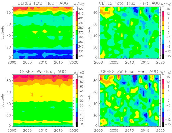
Figure 1.
CERES top of the atmosphere (TOA) flux and perturbations of total (top panels) and SW (bottom panels) for the months of August in 2000–2019.
Figure 1 also reveal a lagged correlation between the mid- and high-latitude flux oscillations with the Arctic fluctuations leading the sub-Arctic (e.g., 60°N) ones by 1~2 years. Since 2009, this lagged relationship has become more evident due to the increased amplitude of Arctic fluctuations. It remains debatable, however, whether the changing Arctic or its increased variabilities can significantly impact the mid-latitude climate or weather systems [10], and vice versa [8]. Although TOA fluxes are not the only factors that drive the near-surface variabilities, these precise measurements are indicative of some key climate-system changes that have caused an additional imbalance in the Arctic at a decadal scale.
The CERES EBAF data also contain monthly cloud fraction (CF) on a 1° × 1° longitude-latitude grid, which is derived essentially from MODIS (Moderate Resolution Imaging Spectroradiometer). As an important variable to interpret the observed variations in the TOA SW flux, CF can have a major influence on how much sunlight is reflected back to space. Although clouds, unlike sea ice and snow cover, do not always occur at the same location, their impacts on the SW flux are realized through the frequency of occurrence, which is effectively integrated in the monthly CF data. The distribution of monthly cloud amount, as well as cloud occurrence frequency, is useful diagnosis variables of the TOA SW variability.
2.2. TOA Albedo Data
Although the CERES EBAF Ed4.1 data are significantly improved over the earlier versions, producing accurate all-sky TOA radiative fluxes requires an algorithm to take into account correction of geostationary-Earth-orbit (GEO) satellite calibration artifacts, CERES–MODIS narrowband-to-broadband (N2B) radiance conversion, and cloud mask and scene classification [14]. In the polar region, the TOA SW flux measurement may subject to greater uncertainty than the middle and lower latitudes due to scene classification and diurnal sampling correction (without GEO). To evaluate and verify the interannual variations in the CERES TOA SW flux, we compared the result with the observations obtained by Multiangle Imaging SprectroRadiometer (MISR) on the same platform but using a very different technique. The comparison is carried out in terms of the TOA albedo, which can be calculated by dividing the reflected TOA SW flux over the incident solar insolation.
Different from the CERES technique, which relies on empirical angular distribution models (ADMs) to convert the single-angle broadband radiance to the TOA flux [15,16], the MISR technique can measure instantaneous ADM at four narrow spectral bands with nine-angular radiance measurements in the along-track direction [17]. To obtain the TOA albedo, however, the MISR technique needs to use modeled N2B functions, which are scene-dependent, to convert its narrow-band radiances to the broadband SW radiances. Thus, the MISR algorithm also requires scene classification. Because the scene classification (into thousands of types) algorithms may differ depending on observing techniques, some differences in the TOA albedo are expected. For example, it is challenging to classify clouds over sea ice. Hence, the two techniques may yield different SW albedos, as the scene type classification can be different. Mountainous terrains with substantial 3D inhomogeneity can be particularly challenging for the techniques that rely on single-view radiance measurements for the SW flux determination.
In addition, CERES and MISR have quite different pixel resolutions (10 km vs. 275 m) and sampling swaths (3000 km vs. 400 km). The larger swath allows CERES to cover both North and South Pole during the summer months while MISR has a gap at latitudes from 84° poleward. Observations from a narrow swath also have a larger sampling error due to fast processes like clouds. Thus, each technique has its own advantages and limitations in handling Arctic atmospheric/surface inhomogeneity and variability, and differences between the two TOA albedo products are expected [e.g., Zhan et al., 2018]. Here, an objective of MISR-CERES albedo intercomparisons is to identify robust and consistent features over the Arctic, Antarctic and Tibetan Plateau, given their sampling and conversion method differences. Because of differences in scene classification, viewing geometry, swath sampling and narrow-vs-broad radiances, verification of independent CERES and MISR measurements provides fidelity of the observed TOA SW features and their variabilities.
This study also compares the observed TOA albedo variations with those derived from the Modern-Era Retrospective analysis for Research and Applications, Version 2 (MERRA-2) and the fifth generation of European Centre for Medium-Range Weather Forecasts (ECMWF) atmospheric reanalyses (ERA5). MERRA-2 derives the TOA radiations fluxes by assimilating available satellite radiance and conventional observations. The MERRA-2 background atmospheric model is the Goddard Earth Observing System model (GEOS) [18]. MERRA-2 is produced on a 5/8° longitude × 1/2° latitude grid in 72 vertical levels. For MERRA-2, the surface representation has been substantially revised from MERRA to include snow hydrology processes, a prognostic albedo, and energy conductivity through snow and ice layers at a high vertical resolution [19]. Other improvements in MERRA-2 include modifications to the representation of turbulence and moisture-related processes. In this study we use the “tavgM_2d_rad_Nx: 2d, monthly mean, 1-hourly time averaged, assimilation, single-level diagnostics V5.12.4 [20], to calculate the TOA albedo. Differences between the TOA incoming solar flux values used by EBAF and the MERRA-2 reanalyses can cause a bias in the TOA SW fluxes. While a ~1 W m−2 SW downward flux adjustment was made for MERRA-2 compared to that of MERRA, there still exists a difference of 6.1 W m−2 in TOA SW upward flux from that of EBAF [21]. In this study we focus primarily on comparisons of the interannual variations from these data sets.
In ERA5, the radiative flux variables have a spatial resolution of ~31 km (0.28125° × 0.28125°) and an hourly temporal resolution [22]. ERA5 uses the Integrated Forecasting System (IFS) with a 4-D variational analysis (4DVAR) assimilation system. We used the ERA5 Top net Solar Radiation (TSR) and Top net Thermal Radiation (TTR) [23].
2.3. Index Data for Arctic Analyses
Arctic sea ice extent (SIE) is one of the key variables that drives the summertime TOA albedo. We use the monthly SIE data archived at the National Snow and Ice Data Center (NSIDC) as an index to characterize the year-to-year variation of sea ice change. As discussed later in the paper, the TOA fluxes will be regressed to the SIE index, to understand its impacts not only on the Arctic but also on the surrounding sub-Arctic and mid-latitude regions.
For this reason, we employ another key regional index, the North Atlantic Oscillation (NAO), which is the difference of atmospheric sea level pressure between the Azores High and the Icelandic Low. Although NAO is derived from regional weather patterns, it has a profound impact on remote area including the Arctic basin. We also employ the Arctic Oscillation (AO) index as a representative of the Northern Annular Mode that describes the annular pattern of atmospheric circulation anomalies across the mid-latitudes and the Arctic. In this study we obtained the monthly NAO index from NOAA National Centers for Environmental Prediction (NCEP).
Cloud and snow cover are important factors that can affect the TOA albedo. To characterize northern hemisphere (NH) cloudiness, we define a cloudiness index (CI) as the gridbox mean CF averaged from latitudes of 55°N–65°N in the CERES EBAF data (see Section 4 for more details). This averaging is weighed by the gridbox area. For snow cover (SC), we use the total SC at latitudes of 40°N poleward, which is derived from MODIS observations [24], as an index to characterize the land area covered by snow. As a secondary effect, ice/snow albedos may differ slightly, depending on their compositions (e.g., aerosol deposition, new/old ice) and mixtures (e.g., ice with leads).
To evaluate impacts of the El Niño-Southern Oscillation (ENSO) on the Arctic TOA fluxes, we employ the NOAA monthly Oceanic Nino Index (ONI) index, which is defined as the average sea surface temperature (SST) anomalies in the Niño 3.4 region (5°S–5°N; 170°W–120°W). Interannual variations at mid-to-high latitudes can be linked remotely to the tropical ocean change through teleconnection processes. Regression to the ONI index will help to quantify such a teleconnection impact. Similarly, a spring-summer-fall pattern in the surface temperatures over East Pacific–North Pacific (EPNP) provides a key index for intense storm activity over the mid-latitudes of the North Pacific [25].
3. Results
The TOA fluxes over the Arctic, Antarctic, and Tibetan Plateau (TP) are experiencing a significant change in recent years due to the vulnerability of their underlying sea ice and snow cover to the regional warming. During 2000–2019, the period with CERES and MISR observations, the global surface temperature has increased by ~0.5 °C and the Arctic by ~1.5 °C [26]. These warming trends as well as interannual variability of the warming play a fundamental role in the observed TOA SW flux.
3.1. Interannual Variabilities
3.1.1. Arctic
The observed mean JJA albedo distribution over the Arctic is shown Figure 2, along with the time series of zonal mean albedo perturbations as a function of latitude from MISR, CERES, ERA5 and MERRA2. Both MISR and CERES observations reveal a similar TOA albedo distribution with the brightest over Greenland and Arctic sea ice. The CERES albedo over the Pacific and Atlantic is mostly from clouds, which is slightly brighter than MISR measurements. On the other hand, MISR albedo perhaps has slightly more variability over landmasses. A decreasing TOA albedo trend is clearly evident in both CERES and MISR JJA data at latitudes greater than 60°N where the Arctic change is dominated by the summer sea ice loss. The lowest Arctic albedo for JJA occurred in 2011 during the two-decade observation period. In addition, there is a strong interannual oscillation on the top of the trend, showing low albedos in 2008, 2011 and 2015 at these latitudes. It is noteworthy that these low-albedo years are one year ahead of the large mass loss anomalies over Greenland Ice Sheet (GrIS) in 2009, 2012 and 2016 [27]. At the 60°N–80°N latitude bin, GrIS is the dominant source of the TOA albedo. Despite their very different remote sensing techniques, CERES and MISR observations reveal an overall consistent pattern of the year-to-year TOA albedo variations at the latitudes (50°N–82°N). This gross consistency provides high fidelity on the TOA SW oscillations as observed by these sensors from 2000 to 2019, as well as the TOA albedo distribution at high latitudes.
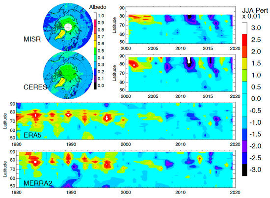
Figure 2.
Time series of CERES, MISR, ERA5 and MERRA2 albedo perturbations for June-August (JJA) between 50°N–90°N. The ERA5 and MERRA2 perturbations are computed using the 2000–2019 mean. The mean albedo distributions observed by MISR and CERES are shown in the upper left maps. In the MISR and CERES panels the perturbations with a value < −0.03 are in white.
Compared to the high-latitude (70°N–80°N) oscillations, the sub-Arctic (60°N–70°N) variations appear to have a lag of 1–2 years. The lagged correlation is more evident after 2011 when the interannual oscillations intensify. The oscillations at latitudes > 70°N show a period of ~4 years during 2006–2019, whereas the lagged oscillations in the sub-Arctic seem to preserve the periodicity during the period after 2011. As discussed above, this lagged albedo variation in Figure 2 is largely driven by the variabilities of GrIS at 65°N and sea ice at 80°N.
The interannual oscillations of TOA albedo in 2000–2019 are captured, to some extent, in the MERRA2 and ERA5 reanalysis data. Similar perturbations in the MERRA2 and ERA5 albedos are found at latitudes < 70°N. However, for latitudes > 70°N the reanalysis data differ from each other substantially. Their differences are much larger than those found between CERES and MISR, indicating problems in the reanalysis at high latitudes. For example, at latitudes > 80°N, the oscillations from MERRA2 and ERA5 even disagree in sign, with MERRA2 more in agreement with the CERES observation. The CERES observations, as well as in the MISR observations up to 82°N, show that the interannual oscillations have a coherent extension to the pole, whereas the ERA5 and MERRA2 reanalysis data exhibit a break at 80°N. Since the albedo at these latitudes come mostly from the sea-ice-covered Arctic Ocean, it raises a question whether some important processes (e.g., melt pond on sea ice) are missing in the underlying model of the reanalysis. The melt pond fraction is one of the key factors needed to determine the heat budget of ice-covered area [28], but it is difficult to measure from space directly.
3.1.2. Antarctic
In the Antarctic the CERES and MISR TOA DJF albedo data show similar interannual variations (Figure 3). Both data sets reveal an albedo increase in 2013–2015 at 65°S, followed by a sharp reversal in 2016. While the 2013–2015 albedo increase is confined near 65°S, the reversal occurs over a wide range of latitudes between 60°–80°S. The 65°S latitude belt is where most of the Antarctic sea ice variability is seen. The dramatic decrease in Antarctic sea ice in 2016 has been intensively studied and attributed potentially to a number of factors including Southern Annular Mode (SAO) and Interdecadal Pacific Oscillation (IPO) [29], as well as Pacific South American (PSA) teleconnection [30].
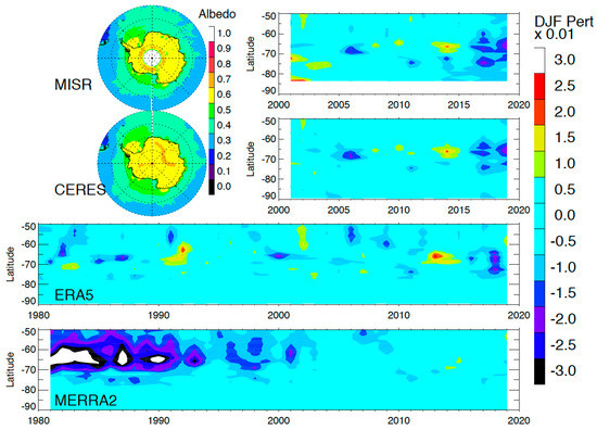
Figure 3.
As in Figure 2 but for December-February (DJF) at latitudes of 50°S–90°S. In MERRA2 the perturbations with a value < −0.03 are in white.
The TOA albedo oscillations induced by the Antarctic sea ice are perhaps represented better by ERA5 than by MERRA2. The 2016 albedo reversal in ERA5 is more consistent with the CERES and MISR observations, but it appears to be delayed by a year. On the other hand, MERRA2 lacks variability in the TOA albedo during 2000–2019. In addition, MERRA2 shows a much larger trend in the earlier period (1980–2000) at 60°S–70°S latitudes, compared to the ERA5 data, indicating a great challenge in these reanalyses to represent the energy balance in the Antarctic.
3.1.3. Tibetan Plateau (TP) and High Mountain Asia (HMA)
Unlike the Arctic and Antarctic, the TP and HMA (e.g., Afghanistan, Pakistan, and Tajikistan) have highly variable terrains where the 3D effects can induce a larger uncertainty than the flat surface cases. Thus, the TP and HMA regions provide a good testbed to verify the TOA albedo observed by CERES and MISR. As shown in Figure 4, the CERES and MISR albedo measurements reveal a similar distribution and interannual variations. Although the CERES albedo values may be slightly higher than MISR, the distribution patterns over the TP and HMA regions are quite consistent between the two data sets.
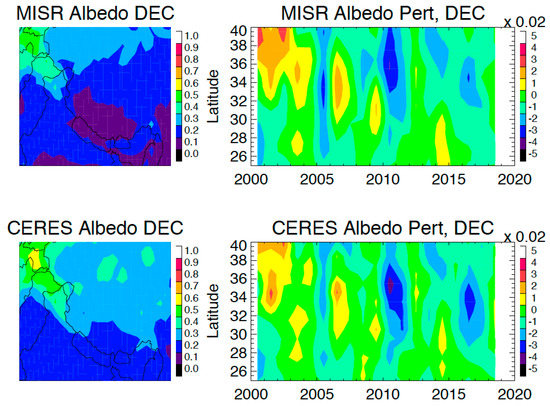
Figure 4.
As in Figure 2 but for December over the Tibetan Plateau (TP) and High Mountain Asia (HMA) regions (70°E–100°E, 25°N–40°N).
The CERES-MISR consistency is perhaps more striking in the observed interannual variations, as these observations have to overcome 3D effects of the complex terrain with very different techniques. December is the month when the largest albedo decreasing trend as well as year-to-year variations are observed by MISR and CERES during 2000–2019. The December oscillations reveal a low albedo in 2005, 2010, and 2016, with a period of ~5 years. The 5-year fluctuation is mixed with a quasi-biennial oscillation on the top of a decreasing trend, driving most of the December variabilities. HMA has the largest glacier and perennial snow cover concentration outside the polar regions. The TOA albedo over the TP and HMA is largely determined by the glacier and snow cover in the region. The MODIS snow cover variation (not shown) is found to be highly correlate with the TOA albedo oscillation seen in Figure 4. Recent studies also show that the snowline altitude at the end of melt season over HMA has been rising during 2001–2016 [31], suggesting a reduction in regional snow cover and surface albedo.
3.2. Trends in 2000–2019
To characterize regional variations of the TOA albedo in further detail, we analyze the observed trends in 2000–2019 on a monthly basis for the Arctic, Antarctic and TP/HMA regions. By breaking down the trend distribution by month, it helps to identify the underlying processes that may evolve with time, in particular those from the surface processes that can vary substantially from month to month and region to region.
As shown in Figure 5, decreasing trends of the TOA albedo dominate everywhere in the Arctic in every month. During June-October the obvious decreasing trend is near the sea ice margin zone where sea ice retreat and early start of the melt season have contributed to the large trend seen in 2000–2019. This trend is narrowly following the margin zone in August-September but widen in October. In May-June a significant trend can also be found in the northern Canada, Victoria and Queen Elizabeth Islands, Beaufort Sea, Laptev Sea, and the eastern Europe, where early snow melt may play a role in reducing the surface albedo. In December a decreasing trend in Europe, particularly over the Alps, reflects a lack of snowfall or snow cover in the recent years.
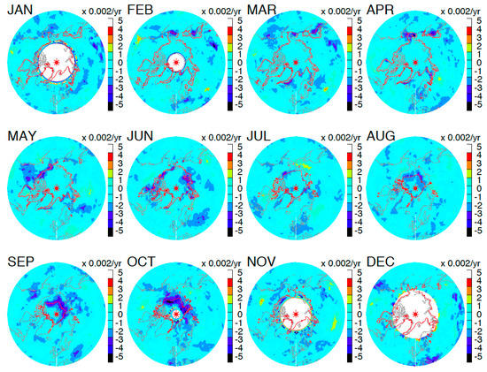
Figure 5.
CERES albedo trend over the Arctic. The uncertainty from fitting is +/−0.002 yr−1 (2σ). The red contours represent the 80% monthly mean sea ice extent.
In Figure 6, the Antarctic TOA albedo is dominated by a decreasing trend in all months, which is largely driven by the sea ice trend [32]. During the summer months (e.g., February) the sea ice extent retreats near the coastal line (~67°S), whereas in the winter months (e.g., September) it expands to the latitudes of ~60°S. The decreasing trend over West Antarctica is quite persistent during November-April, which is consistent with the report from CryoSat-2 that the West Antarctic Ice Sheet (WAIS) is disappearing [33]. Over East Antarctica, the decreasing trends appear to be associated with the sea ice margin zones, moving from the Southern and Indian Ocean in August-November to Weddell Sea in December-January. There is a significant decreasing trend over the Atlantic Ocean in September and December, which is likely due to cloudiness changes. Compared to the decreases in sea-ice-induced TOA albedo, the cloud effects are more scattered and diffused in a wider area. Finally, a significant trend is observed over the Chilean Patagonia during the winter-spring months (June-October), which seems to be related to the decreases in snow cover from high-altitude warming [34].
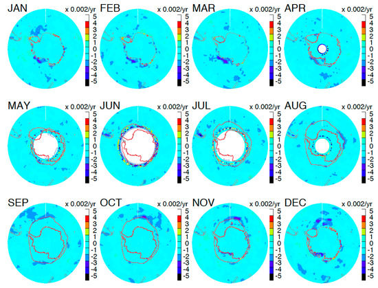
Figure 6.
As in Figure 5 but for the Antarctic.
As demonstrated in Figure 4, the consistent TOA albedo observations from CERES and MISR over the TP and HMA allow more quantitative assessment of the regional trend over these mountainous areas. June-August (JJA) is the TP’s wet season, followed by a dry season in September-November (SON) [35]. An enhanced warming in TP is strongly coupled with surface albedo changes [36]. HMA gets its most precipitation in December-February (DJF) whereas Taklamakan receives its mostly in March-May (MAM). During its growing season (May-September) decreasing trends in June and August are observed in the central and eastern TP (Figure 7). The decreasing albedo could be caused by a number of factors including the enhanced evapotranspiration cooling on vegetation [37], black carbon (BC) and dust aerosols on glaciers [38], and increases of atmospheric anthropogenic aerosols [39]. There are decreasing trends in November and January over the eastern TP region (e.g., Bhutan, Myanmar and Bangladesh), which is likely related to the observed decreases in snow cover [40] and glacier area [41].
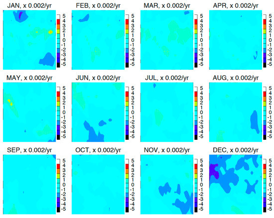
Figure 7.
CERES TOA albedo trend over Tibetan Plateau (TP) and High Mountain Asia (HMA).
The decreasing trend over HMA in December is highly correlated with the decreasing snow cover [42] and the shrinking glacier area in the region [42,43]. The glacier losses appear to accelerate in the 21st century with a higher rate at lower elevations [44]. The thinning glaciers [45] and reduced snowfall [46] in HMA region may have all contributed to the reduction of surface albedo, which results in the decreasing trend in the TOA albedo.
4. Discussion
In this section we attempt to provide a further analysis on the attributions of the interannual variations of Arctic summertime TOA fluxes. We focus on components that contribute most to the total variances seen in 2000–2019 at latitudes of 40°N poleward, such as spatial climatological patterns and weather indices. Two methods are employed to break down the total variability: empirical orthogonal function (EOF) analysis and climate index regression. The EOF analysis will provide the orthogonal variation patterns that yield the most contribution to the total variance, but will not provide any attributions to the physical parameter/process responsible for the derived patterns. On the other hand, the index regression will help sort out the contributions and their correlation to each physical index/process, but may not capture most of the variances in Arctic TOA fluxes. In addition, indices may not be fully independent of each other, which can lead to a large unwanted covariance.
4.1. Leading EOF Patterns
Figure 8 shows three of the five leading EOF patterns of the CERES total, LW and SW TOA fluxes. As seen in Table 1, the five EOFs contribute about ~50% of the total variance from latitudes of 40°N poleward, whereas the combination of the first three EOFs gives ~32%. It would take 10 EOFs to capture ~73% and 18 EOFs for ~98% of the total variance. After EOF#5, the variance tends to fall exponentially as a function of , where N is the EOF number and b is an empirical coefficient that can be found in Table 1.
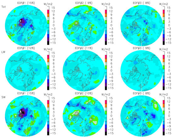
Figure 8.
Leading three empirical orthogonal function (EOF) patterns of CERES TOA fluxes for JJA. The sum of three leading EOFs represents 32%, 32% and 33% of the total variance in total (TOT), LW, and SW fluxes, respectively.

Table 1.
Percentage of CERES TOA flux variance (40°N poleward) in EOFs.
These EOFs are derived with an area-weighted analysis, and the first EOF takes 16%, 13% and 15% of the variance respectively for total, LW and SW fluxes. Without weighted by area, the EOFs would be biased to the variabilities at high latitudes, for which the first EOF would capture as more variance as 24%, 19% and 23% respectively. Note that the amplitudes and patterns of the EOFs in the total and SW fluxes are similar and comparable, indicating that the total TOA flux variability is dominated by the SW. The LW EOF patterns generally have an opposite sign to the SW ones, providing a damping effect to the SW forcing. As discussed later in this section, clouds play a major role in creating such an offset effect.
A significant portion of EOF#1 can be explained by the TOA flux anomaly distributions associated with the variation of NAO phase. The temporal correlation between the time series of EOF#1 PC and summertime NAO index is high: −0.79 (total), −0.51 (LW), and −0.76 (SW). The high NAO-EOF#1 correlation suggests a broad influence of the negative phase of the NAO on the total and SW flux anomalies over the Arctic, which extends to Greenland as seen in EOF#1 (left column of Figure 8). This characteristic feature will be discussed again in Section 4.3. EOF#2 may have a moderate relationship with the EPNP that generally accounts for the large-scale mass/circulation changes across the Northeast Pacific/Alaska and Northern Canada (e.g., Archipelago region). The correlations between the PC time series and the EPNP index are 0.34 (total) and 0.32 (SW). Although the correlation values are not remarkably high, the impact of EPNP appears to be reflected in the EOF#2 pattern, as negative anomalies of total and SW flux along the North America northwest coast and positive anomalies over Northern Canada. Such an oscillating pattern corresponds to the positive phase of EPNP.
While there is no significant trend in the time series of EOF#1 and #2 (Figure 9), the PC amplitudes of EOF#3 in 2000–2019 do exhibit a significant trend. The EOF#3 patterns in Figure 9 indicate the vulnerable regions of the future SW flux variation if the albedo continues to decrease. One of these regions is the western Greenland and northern Canada where the SW flux or albedo had been decreasing in 2000–2019. The other regions, which appear in a wavy pattern, include Europe (decreasing), Finland (increasing), Russia (decreasing), the northeastern China (increasing), and Kara and Beaufort Seas (decreasing). Despite the small (8%) contribution of EOF#3, its trend amplitude must not be neglected since it may reveal severe impacts of the underlying processes (e.g., sea ice loss) on these regions.
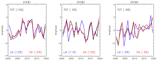
Figure 9.
Time series of the amplitude of three leading EOF principal components (PCs).
4.2. Impacts of Cloud Cover
Clouds play a significant role in the overall Arctic and subarctic TOA albedo and its variability. While cloud cover may vary from year to year in response and/or feedback to the changes from atmospheric, hydrological and cryospheric processes, their contributions to the TOA SW flux are more than the surface contributors such as those from Arctic sea ice and Greenland ice sheet (GrIS) changes [47].
The authors of Figure 10, characterize the importance of cloud cover by mapping out the correlation between the TOA SW flux and the monthly gridded cloud fraction (CF) from the CERES EBAF data. The climatological mean distributions of the SW flux and CF resemble each other over the regions without sea ice and outside Greenland. The year-to-year variabilities of the CF and SW flux are highly correlated in these regions with the exception of those where the mean CF becomes greater than 90%, such as the Pacific and Atlantic storm tracks. Because these high-CF regions are constantly covered by clouds, it is expected that cloud-saturated regions produce a smaller year-to-year variation. On the other hand, the regions with less-saturated CF, such as landmasses, had experienced a relatively large CF variability that is correlated with the SW flux fluctuations. As expected, the regions covered by sea ice and permanent ice sheets have a low correlation with CF.
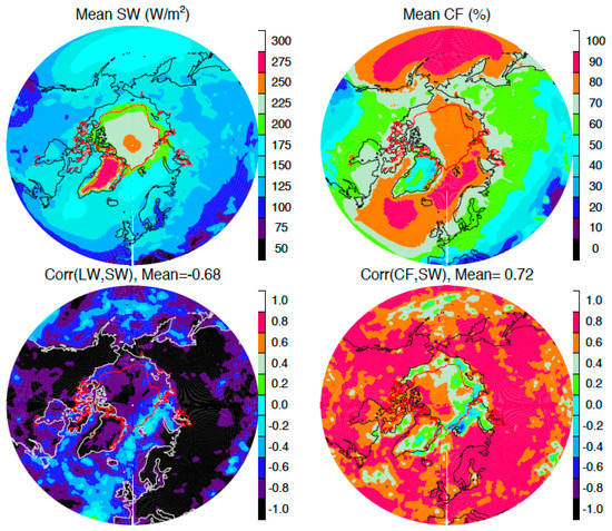
Figure 10.
CERES mean TOA SW flux and cloud fraction (CF) distributions for JJA (top panels), and correlation maps between year-to-year variations in the LW and SW fluxes and between CF and SW (bottom panels) at latitudes of 40°N poleward. The red contour is the JJA mean sea ice extent at 80%. The regional mean correlation coefficients are indicated in the label of the bottom panels, showing dominated anti-correlation between LW and SW and positive correlation between CF and SW.
In the regions where CF and SW are highly correlated, the TOA SW and LW fluxes are anti-correlated, suggesting that cloudy-sky produces less outgoing LW radiation. In other words, the cloud top temperature in JJA is generally colder than the clear-sky surface temperature. This anti-correlation between the LW and SW fluxes is found mostly over land and near the coasts, where the cold cloud top and warm surface conditions are often valid. Again, the LW and SW correlation is poor in the regions where CF is greater than 90%.
Because CF is highly correlated with the SW flux in the subarctic regions, we create a cloudiness index (CI) to represent the gridbox mean CF at latitudes of 55°N–65°N using the CERES EBAF data. As seen in Figure 10, this CI index is designed to capture most of the cloud-induced SW variabilities over the subarctic landmasses,
4.3. Impacts of SIE, SC, NAO, ONI, CI, EPNP, and AO
Since the EOF analysis cannot provide clear attribution to what physical processes are responsible for the interannual oscillations seen in the TOA flux data, we regress CERES TOA fluxes to several climate indices, namely, SIE, SC, NAO, ONI, CI, EPNP, and AO, to evaluate their connection to the Arctic flux variations. SIE, SC, an CI can directly affect the TOA albedo because of relatively high albedos from sea ice, snow and clouds. Other atmospheric (e.g., water vapor, aerosol) and surface (e.g., wetlands, vegetation, melt ponds) variables may directly or indirectly alter the TOA albedo. Collectively, these albedo contributors are subject to atmospheric, hydrological, and cryospheric processes, which can hardly be represented by a single dynamical index. Climatologically, the NAO, ONI, EPNP, and AO indices are found to have a significantly influence on the NH mid-to-high latitudes.
In Figure 11, the authors show the time series of these indices in 2000–2019 during which only SIE exhibits a significant trend. Two strong peaks in NAO since 2010 are separated by ~4 years, which are apparently cross-correlated with the oscillations in CI and SC. The cross correlation among indices implies the existence of a significant covariance and mutual dependence on similar underlying process(es). Another cross-correlation example is shown in Figure 12 where the zonal mean CF has latitude-dependent correlation with the AO and ONI indices. It suggests that CFs in the core of arctic (75°N–90°N) are highly correlated with AO while CFs are more correlated with ONI in the subarctic region (65°N–75°N).
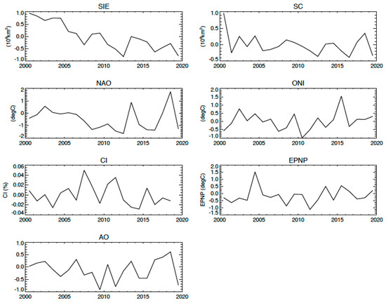
Figure 11.
Major indices used in the correlation analysis for the Arctic TOA fluxes during JJA: Arctic sea ice extent (SIE), snow cover (SC), Northern Atlantic oscillation (NAO), oceanic niño index (ONI), mean 1° × 1° cloudiness index (CI) at 55°N–65°N latitudes, Pacific - North Pacific (EPNP), and Arctic oscillation (AO).
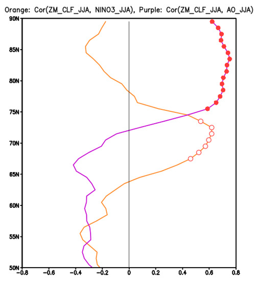
Figure 12.
Correlation between zonal mean CF and AO (purple) and ENSO (orange) in JJA as a function of latitude. Red and orange dots indicate statistical significance at the 95% confidence level.
Despite no significant dominance from each individual index, NAO, CI, and SIE are found to contribute most to the Arctic TOA flux variations, followed by ONI and EPNP (Table 2). For the TOA SW flux, the designated CI outperforms NAO to make the most contribution. For the surface upward SW flux, which can be obtained from the CERES EBAF data, SIE provides the most contribution (24%) as expected for the dominant surface process associated with the Arctic sea ice loss. The combined contribution from the seven indices (SIE, NAO, CI, SC, ONI, EPNP, and AO) counts for ~47% of TOA total and SW flux variance. Similarly, the surface SW flux covered by multiple indices can go up to 56%.
Table 2.
Percentage of CERES TOA flux variance (40°N poleward) represented by regression to the indices (SIE, NAO, CI, SC, ONI, EPNP, and AO) in JJA.
The correlation maps of the TOA fluxes with these indices reveal the regions where each index has most impacts (Figure 13). For SIE, strong correlations with the total and SW fluxes are seen over the Arctic sea ice margin zone as well as over Greenland and Russia. The LW flux has strong anti-correlation with SIE over Greenland, Russia and Northern Canada, but not much over the sea ice margin zone.
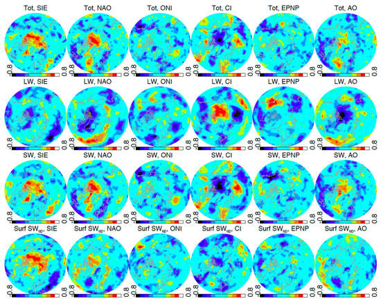
Figure 13.
Correlation coefficient maps of CERES JJA TOA fluxes with the major indices (except snow cover) of interest.
NAO produces overall strong positive correlation with the total and SW fluxes over the Arctic Ocean, Greenland and Northern Canada, but anti-correlated with the LW flux in these regions. In the northern Europe, NAO is negatively correlated with the total and SW fluxes, with a slightly positive correlation with the LW flux.
4.4. Interactions between Mid- and High-Latitude Disturbances
The observed TOA radiation changes indicate a significant imbalance of the summer Arctic energy on an interannual-to-decadal time scale. The oscillatory patterns seen in Figure 1 between mid- and high-latitudes suggest some complex teleconnection or coupled processes at work. The lagged correlation between subarctic and Arctic TOA fluxes indicates potential influences of Arctic sea ice loss on subarctic climate on an interannual scale. To further characterize the coupling between low and high latitude variations, here we apply a two-dimensional (2D) Fast Fourier Transform (FFT) decomposition method to the oscillatory patterns in Figure 1, and derive the poleward and equatorward progressing components. As a typical spectral analysis, this FFT method splits the input 2D wave into standing, y+ (poleward) and y− (equatorward) components, where the x-axis is time. For the August TOA SW flux, the equatorward component has the higher contribution with 41% of the variance, compared to 29% and 28% of the standing and poleward components.
The connection between mid- and high-latitude oscillations becomes much clearer in the decomposed equatorward and poleward components with extended coherent patterns (Figure 14). The Arctic influence on the TOA SW flux is more pronounced in the equatorward component, showing coherent perturbation patterns extending as low as ~50°N. For comparison, we applied the same decomposition analysis to the CERES CF data and find the similar patterns. At high latitudes the interannual oscillations of equatorward component of both SW flux and CF appear to intensify after 2009 as seen the original unsplit SW data. The poleward component shows the strong years in 2006–2008.
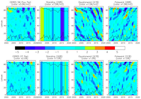
Figure 14.
CERES TOA SW flux (top panels) and CERES CF (bottom panels) perturbations for the month of August as a function of time and NH latitude, along with the decomposed standing, equatorward and poleward components with their relative contribution in percentage. The SIE and ONI indices are overplotted at the top and bottom of each panel, respectively.
In the tropics and subtropics, both SW and CF show significant coherent patterns in the equatorward component during 2003–2007 and 2013–2017. It is worth noting that Europe experienced some of the worst heat waves in the summer of 2003 and 2015, which in both cases came 2 years after a strong TOA SW anomaly at the mid-latitudes. How the heat wave patterns are related interannually between different regions warrants a further investigation. For the poleward component, the SW flux and CF have a relatively weak influence from mid to high latitudes, nor significant influence extended from the tropical ENSO.
5. Conclusions
In this study we compared the TOA albedo observed by MISR and CERES in 2000–2019 over the Arctic, the Antarctic and the HMA/TP (High Mountain Asia and Tibetan Plateau), and found generally consistent distributions and interannual variabilities, despite the fact that the observations were made from very different remote sensing techniques. It remains challenging to make reliable observations of the TOA fluxes from space, because the assumptions used in the retrievals for angular distribution functions (ADMs) and narrow-to-broadband (N2B) conversion can subject to various issues at high latitudes. Scene type classification, complex 3D surface topography, spatiotemporal sampling differences can all contribute to errors or differences of the albedo measurement made by MISR and CERES.
Despite these limitations and different observing techniques, both CERES and MISR data showed consistent TOA albedo distribution and interannual variations over high latitudes, as well as over HMA/TP, which provided high fidelity about the observed patterns. Several salient features emerge from these measurements:
- A summertime TOA albedo decreasing trend is consistently seen in both MISR and CERES data at latitudes greater than 60°N where the Arctic change is dominated by the summer sea ice loss. The lowest Arctic albedo for JJA occurred in 2011 during the two-decade observation period.
- Similar Arctic interannual oscillations are found in MISR and CERES JJA albedo data, showing low albedos in 2008, 2011 and 2015 at high latitudes, which are approximately one year ahead of the large mass loss anomalies over GrIS in 2009, 2012 and 2016. This led to a lagged (1–2 years) correlation between the high-latitude (70°N–80°N) and the sub-Arctic (60°N–70°N) variations in the zonal mean TOA albedo.
- In the Antarctic MISR and CERES both reveal an albedo increase in 2013–2015 at 65°S, followed by a sharp reversal in 2016. The 2013–2015 albedo increase is confined in a narrow latitude band near 65°S, but the reversal in 2016 occurred over a wide range of latitudes between 60°–80°S.
- Despite potential 3D effects of the TP/HMA complex terrain on the TOA flux observations, the observed albedo variations and distributions by MISR and CERES are strikingly consistent with each other. December is the month with the largest albedo decreasing trend and associated with a 5-year fluctuation.
We further evaluated ERA5 and MERRA2 TOA SW fluxes with the MISR and CERES observations. It was found that at high latitudes there are large discrepancies between the CERES/MIRS TOA albedo and ERA5/MERRA2 reanalyses, suggesting a serious shortcoming in these advanced reanalyses in terms of representing polar energy budget. These reanalyses failed to capture the lagged relation between the Arctic and subarctic TOA SW fluxes, and in some cases they produced an out-of-phase variations compared to the observations. The observed fluctuations of Arctic TOA fluxes have a quasi-4-year period during 2000–2019 and appear to intensify after 2009.
Sea ice and cloud variabilities dominate year-to-year variations of the high-latitude TOA albedo. In the Arctic the CI, NAO, and SIE contribute most to the interannual variation, for which the PC variation of the first EOF is highly correlated with the NAO index. In the Antarctic, MERRA2 lacks the TOA SW variability induced by sea ice changes during 2000–2019, whereas ERA5 generally performs better in representing this variability.
We applied an 2D-FFT analysis to decompose the interannual variations of the Arctic TOA fluxes in the time and latitude domain. The method helps to reveal a clearer polar influence on the subarctic climate, as well as the lagged relationship between the mid and high latitudes.
Author Contributions
Conceptualization, D.L.W., J.N.L.; methodology, D.L.W.; software, D.L.W.; validation, D.L.W., K.-M.K., Y.-K.L.; formal analysis, D.L.W., K.-M.K., Y.-K.L.; investigation, D.L.W., J.N.L., K.-M.K., Y.-K.L.; resources, D.L.W.; data curation, D.L.W., K.-M.K.; writing—original draft preparation, D.L.W.; writing—review and editing, D.L.W., J.N.L., K.-M.K., Y.-K.L.; visualization, D.L.W., K.-M.K.; All authors have read and agreed to the published version of the manuscript.
Funding
This research was supported by NASA’s Sun-Climate research fund to Goddard Space Flight Center.
Acknowledgments
The CERES and MISR data were obtained from the NASA Langley Research Center Atmospheric Science Data Center.
Conflicts of Interest
The authors declare no conflict of interest.
References
- Parkinson, C.L. A 40-y record reveals gradual Antarctic sea ice increases followed by decreases at rates far exceeding the rates seen in the Arctic. Proc. Natl. Acad. Sci. USA 2019, 116, 14414–14423. [Google Scholar] [CrossRef] [PubMed]
- Kwok, R.; Cunningham, G.F.; Wensnahan, M.; Rigor, I.; Zwally, H.J.; Yi, D. Thinning and volume loss of the Arctic Ocean sea ice cover: 2003–2008. J. Geophys. Res. Oceans 2009, 114. [Google Scholar] [CrossRef]
- Liu, J.; Curry, J.A.; Wang, H.; Song, M.; Horton, R.M. Impact of declining Arctic sea ice on winter snowfall. Proc. Natl. Acad. Sci. USA 2012, 109, 4074–4079. [Google Scholar] [CrossRef] [PubMed]
- Hartmann, D.L.; Ceppi, P. Trends in the CERES dataset, 2000–2013: The effects of sea ice and jet shifts and comparison to climate models. J. Clim. 2014, 27, 2444–2456. [Google Scholar] [CrossRef]
- Wu, D.L.; Lee, J.N. Arctic low cloud changes as observed by MISR and CALIOP: Implication for the enhanced autumnal warming and sea ice loss. J. Geophys. Res. 2012, 117, D07107. [Google Scholar] [CrossRef]
- Pistone, K.; Eisenman, I.; Ramanathan, V. Albedo decrease due to Arctic sea ice loss. Proc. Natl. Acad. Sci. USA 2014, 111, 3322–3326. [Google Scholar] [CrossRef]
- Zelinka, M.; Hartmann, D.L. Climate feedbacks and their implications for poleward energy flux changes in a warming climate. J. Clim. 2012, 25, 608–624. [Google Scholar] [CrossRef]
- Lim, Y.-K.; Cullather, R.I.; Nowicki, S.M.J.; Kim, K.-M. Inter-relationship between subtropical Pacific sea surface temperature, Arctic sea ice concentration, and North Atlantic Oscillation in recent summers. Sci. Rep. 2019, 9, 3481. [Google Scholar] [CrossRef]
- Screen, J.A. Influence of Arctic sea ice on European summer precipitation. Environ. Res. Lett. 2013, 8, 044015. [Google Scholar] [CrossRef]
- Francis, J.; Skific, N. Evidence linking rapid Arctic warming to mid-latitude weather patterns. Philos. Trans. R. Soc. A 2015, 373, 20140170. [Google Scholar] [CrossRef]
- Matsumura, S.; Kosaka, Y. Arctic–Eurasian climate linkage induced by tropical ocean variability. Nat. Commun. 2019, 10, 3441. [Google Scholar] [CrossRef] [PubMed]
- Lenaerts, J.T.M.; Van Tricht, K.; Lhermitte, S.; L’ecuyer, T. Polar clouds and radiation in satellite observations, reanalyses, and climate models. Geophys. Res. Lett. 2017, 44, 3355–3364. [Google Scholar] [CrossRef]
- Loeb, N.G.; Kato, S.; Su, W.; Wong, T.; Rose, F.G.; Doelling, D.R.; Norris, J.R.; Huang, X. Advances in understanding top-of-atmosphere radiation variability from satellite observations. Surv. Geophys. 2012, 33, 359–385. [Google Scholar] [CrossRef]
- Loeb, N.G.; Doelling, D.; Wang, H.; Su, W.; Nguyen, C.; Corbett, J.G.; Liang, L.; Mitrescu, C.; Rose, F.G.; Kato, S. Clouds and the Earth’s Radiant Energy System (CERES) Energy Balanced and Filled (EBAF) top-of-atmosphere (TOA) Edition-4.0 data product. J. Clim. 2018, 31, 895–918. [Google Scholar] [CrossRef]
- Loeb, N.G.; Kato, S.; Loukachine, K.; Manalo-Smith, N. Angular distribution models for top-of-atmo- sphere radiative flux estimation from the clouds and the earth’s radiant energy system instrument on the Terra satellite. Part I: Methodology. J. Atmos. Oceanic Technol. 2005, 22, 338–351. [Google Scholar] [CrossRef]
- Su, W.; Corbett, J.; Eitzen, Z.; Liang, L. Next-generation angular distribution models for top-of-atmosphere radiative flux calculation from CERES instruments: Methodology. Atmos. Meas. Tech. 2015, 8, 611–632. [Google Scholar] [CrossRef]
- Diner, D.J.; Davies, R.; Varnai, T.; Moroney, C.; Borel, C.; Gerstl, S.A.W.; Nelson, D.L. Multiangle Imaging Sprectro Radiometer (MISR) Level 2 Top-of-Atmosphere Albedo Algorithm Theoretical Basis; JPL Report D-13401, Revision D.; Jet Propulsion Laboratory: Pasadena, CA, USA, 1999; 88p. [Google Scholar]
- Molod, A.; Takács, L.; Suárez, M.; Bacmeister, J. Development of the GEOS-5 atmospheric general circulation model: Evolution from MERRA to MERRA2. Geosci. Model Dev. 2015, 8, 1339–1356. [Google Scholar] [CrossRef]
- Cullather, R.I.; Nowicki, S.M.J.; Zhao, B.; Suarez, M.J. Evaluation of the surface representation of the Greenland Ice Sheet in a general circulation model. J. Clim. 2014, 27, 4835–4856. [Google Scholar] [CrossRef]
- Bosilovich, M.G.; Akella, S.; Coy, L.; Cullather, R.; Draper, C.; Gelaro, R. MERRA-2: Initial Evaluation of the Climate; NASA Technical Report Series on Global Modeling and Data Assimilation; NASA/TM-2015-104606; Koster, R.D., Ed.; 2016; Volume 43, 145p. Available online: https://gmao.gsfc.nasa.gov/pubs/docs/Bosilovich803.pdf (accessed on 31 March 2020).
- Hinkelman, L.M. The global radiative energy budget in MERRA and MERRA-2: Evaluation with respect to CERES EBAF data. J. Clim. 2019, 32, 1973–1994. [Google Scholar] [CrossRef]
- Hans, H.; Dick, D. ERA5 Reanalysis Is in Production. 2016. Available online: https://www.ecmwf.int/en/newsletter/147/news/era5-reanalysis-production (accessed on 31 March 2020).
- Hogan, R. Radiation Quantities in the ECMWF Model and MARS. 2015. Available online: https://www.ecmwf.int/node/18490 (accessed on 31 March 2020).
- Hall, D.K.; Riggs, G.A.; Salomonson, V.V. MODIS/Terra Snow Cover 5-Min L2 Swath 500m, Version 5; NASA National Snow and Ice Data Center Distributed Active Archive Center: Boulder, CO, USA, 2006. [Google Scholar] [CrossRef]
- Bell, G.; Janowiak, J. Amospheric circulation associated with the Midwest floods of 1993. Bull. Am. Meteor. Soc. 1995, 76, 681–695. [Google Scholar] [CrossRef]
- Blunden, J.; Arndt, D.S. State of the climate in 2018. Bull. Am. Meteor. Soc. 2019, 100, Si–S305. [Google Scholar] [CrossRef]
- Tedesco, M.; Fettweis, X. Unprecedented atmospheric conditions (1948–2019) drive the 2019 exceptional melting season over the Greenland ice sheet. Cryosphere Discuss. 2019. in review. [Google Scholar] [CrossRef]
- Kashiwase, H.; Ohshima, K.I.; Nihashi, S.; Hajo, E. Evidence for ice-ocean albedo feedback in the Arctic Ocean shifting to a seasonal ice zone. Nature 2017, 7, 8170. [Google Scholar] [CrossRef] [PubMed]
- Meehl, G.A.; Arblaster, J.M.; Chung, C.T.Y.; Holland, M.M.; Duvivier, A.K.; Thompson, L.; Yang, D.; Bitz, C.M. Sustained ocean changes contributed to sudden Antarctic sea ice retreat in late 2016. Nat. Commun. 2019, 10, 14. [Google Scholar] [CrossRef]
- Irving, D.; Simmonds, I.H. A new method for identifying the Pacific-South American pattern and its influence on regional climate variability. J. Clim. 2016, 29, 6109–6125. [Google Scholar] [CrossRef]
- Tang, Z.; Wang, X.; Wang, J.; Wang, X.; Wei, J. Investigating spatiotemporal patterns of snowline altitude at the end of melting season in High Mountain Asia, using cloud-free MODIS snow cover product, 2001–2016. Cryosphere Discuss. 2019. [Google Scholar] [CrossRef]
- Holland, P.R. The seasonality of Antarctic sea ice trends. Geophys. Res. Lett. 2014, 41, 4230–4237. [Google Scholar] [CrossRef]
- Shepherd, A.; Gilbert, L.; Muir, A.; Konrad, H.; McMillan, M.; Slater, T.; Briggs, K.H.; Sundal, A.V.; Hogg, A.; Engdahl, M.E. Trends in Antarctic Ice Sheet elevation and mass. Geophys. Res. Lett. 2019, 46, 8174–8183. [Google Scholar] [CrossRef]
- Pérez, T.; Mattar, C.; Fuster, R. Decrease in snow cover over the Aysén River catchment in Patagonia. Chile. Water 2018, 10, 619. [Google Scholar] [CrossRef]
- Maussion, F.; Scherer, D.; Mölg, T.; Collier, E.; Curio, J.; Finkelnburg, R. Precipitation seasonality and variability over the Tibetan Plateau as resolved by the high Asia reanalysis. J. Clim. 2014, 27, 1910–1927. [Google Scholar] [CrossRef]
- Liu, X.; Cheng, Z.; Yan, L.; Yin, Z.-Y. Elevation dependency of recent and future minimum surface air temperature trends in the Tibetan Plateau and its surroundings. Glob. Planet. Chang. 2009, 68, 164–174. [Google Scholar] [CrossRef]
- Shen, M.; Piao, S.; Jeong, S.-J.; Zhou, L.; Zeng, Z.; Ciais, P.; Chen, D.; Huang, M.; Jin, C.-S.; Li, L.; et al. Evaporative cooling over the Tibetan Plateau induced by vegetation growth. Proc. Natl. Acad. Sci. USA 2015, 112, 9299–9304. [Google Scholar] [CrossRef] [PubMed]
- Qu, B.; Ming, J.; Kang, S.; Zhang, G.-S.; Li, Y.-W.; Li, C.-D.; Zhao, S.-Y.; Ji, Z.-M.; Cao, J.-J. The decreasing albedo of the Zhadang glacier on western Nyainqentanglha and the role of light-absorbing impurities. Atmos. Chem. Phys. 2014, 14, 11117–11128. [Google Scholar] [CrossRef]
- Jia, A.; Liang, S.; Wang, D.; Jiang, B.; Zhang, X. Air pollution slows down surface warming over the Tibetan Plateau. Atmos. Chem. Phys. 2020, 20, 881–899. [Google Scholar] [CrossRef]
- Gurung, D.R.; Kulkarni, A.V.; Giriraj, A.; Aung, K.S.; Shrestha, B. Monitoring of seasonal snow cover in Bhutan using remote sensing technique. Curr. Sci. 2011, 101, 1364–1370. [Google Scholar]
- Cogley, J. Glacier shrinkage across High Mountain Asia. Ann. Glaciol. 2016, 57, 41–49. [Google Scholar] [CrossRef]
- Bolch, T.; Shea, J.; Liu, S.-Y.; Azam, M.F.; Gao, Y.; Gruber, S.; Immerzeel, W.; Kulkarni, A.; Li, H.; Tahir, A.; et al. Status and Change of the Cryosphere in the Extended Hindu Kush Himalaya Region. In The Hindu Kush Himalaya Assessment; Wester, P., Mishra, A., Mukherji, A., Shrestha, A., Eds.; Springer: Cham, Switzerland, 2019. [Google Scholar]
- Brun, F.; Berthier, E.; Wagnon, P.; Kääb, A.; Treichler, D. A spatially resolved estimate of High Mountain Asia glacier mass balances from 2000 to 2016. Nat. Geosci. 2017, 10, 668–673. [Google Scholar] [CrossRef]
- Maurer, J.M.; Schaefer, J.; Rupper, S.; Corley, A. Acceleration of ice loss across the Himalayas over the past 40 years. Sci. Adv. 2019, 5, eaav7266. [Google Scholar] [CrossRef]
- Gardner, A.; Moholdt, G.; Cogley, J.G.; Wouters, B.; Arendt, A.; Wahr, J.; Berthier, E.; Hock, R.; Pfeffer, W.T.; Kaser, G.; et al. A reconciled estimate of glacier contributions to sea level rise: 2003 to 2009. Science 2013, 340, 852–857. [Google Scholar] [CrossRef]
- Kapnick, S.B.; Delworth, T.L.; Ashfaq, M.; Malyshev, S.; Milly, P.C.D. Snowfall less sensitive to warming invKarakoram than in Himalayas due to a unique seasonal cycle. Nat. Geosci. 2014, 7, 834–840. [Google Scholar] [CrossRef]
- Sledd, A.; L’Ecuyer, T. How much do clouds mask the impacts of arctic sea ice and snow cover variations? different perspectives from observations and reanalyses. Atmosphere 2019, 10, 12. [Google Scholar] [CrossRef]
© 2020 by the authors. Licensee MDPI, Basel, Switzerland. This article is an open access article distributed under the terms and conditions of the Creative Commons Attribution (CC BY) license (http://creativecommons.org/licenses/by/4.0/).