The Analysis of Experimental Deployment of IGLUNA 2019 Trans-Ice Longwave System

Abstract

An experimental longwave system operating in the broadcasting spectrum with horizontal magnetic loop transmitting antennas is presented as an element of simulated lunar astronaut mission of the IGLUNA program of Swiss Space Center (ESA_Lab demonstrator) in June 2019 on the Klein Matterhorn glacier in Switzerland. The parameters of the antennas, the environment, the transmitter design, and propagation tests are presented. The best-suited propagation model is developed. As the system, using low powers, provided coverage of maximal distance of 2077.06 km, a single radio station of this type would cover about 36% of the Moon’s surface and allow in situ ground-penetrating research.

1. Introduction

As the return of manned spacecraft to the Moon is predicted to take place as soon as the 2020s, new technology concepts and skilled human resources need to be created to support this process in a long-time perspective. One of the answers to these needs is the IGLUNA ESA_Lab demonstrator project, launched by the Swiss Space Center in 2018 and aimed at university students from European countries [1].

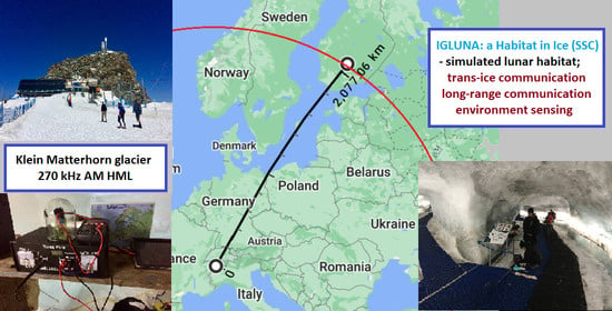
The 2019 (first) edition of IGLUNA took part in June 2019 in Zermatt, Switzerland, and comprised of two main venues: a mission to simulate a lunar habitat and surface operations on the Klein Matterhorn glacier and an exposition of conceptual designs of future lunar equipment in Zermatt’s downtown. Among the student teams involved in the mission part of the initiative, the team P14 from Warsaw University of Technology, Poland, designed equipment responsible for providing radio communication on the surface of the glacier-for the ‘astronauts’ during simulated extravehicular activities—EVAs—and through the glacier into the simulated lunar habitat [2].

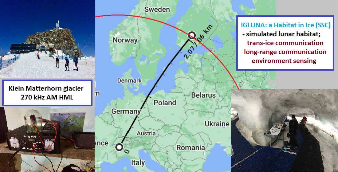
The surface radio communication system consisted of a 2.4-GHz network with mobile transceiver mounted on the astronaut’s vambrace–it allowed the transmission of simple commands and telemetry data. The trans-ice communication system, connecting the EVA region with the habitat located 15 m below, inside the Glacier Paradise ice caves, consisted of two large antennas with separate transmitters and mobile receivers, forming a communication channel with the carrier frequency of 270 kHz (see schematic on Figure 1). As the designed channel was to overcome the main obstacle of the ice ceiling of the Glacier Palace, the preferred transmitting antenna type was determined as the magnetic loop—similar to the antennas of in-body implants, which allow the signal crossing of the tissue (highly humid, aqueous barrier) by employing the less-attenuated magnetic compound of the EM field created by two coaxially-placed loop radiators, functioning simultaneously as transmitting- and receiving ends [3], or antennas used for sub-surface communication systems for various data transmission—the majority of such systems used in deep caves [4] or mines [5], also employing magnetic antennas and LF/VLF frequency ranges for monitoring and rescue services (speleologists and miners). A large project also incorporating a loop antenna employing large terrain features was carried out in New Zealand in 1993 [6], yet with vertical polarization (VML—vertical magnetic loop), different frequency range and different (fully rocky) environment.

Antennas deployed in the aforementioned cases were, however, used mainly in deep underground environments, with coal or solid rocks as surroundings—in the IGLUNA 2019 case, the surroundings were relatively thin (much shorter than the wavelength), icy, and positioned highly above the surface of the Earth. Nevertheless, the prevailing arguments for the HML (horizontal magnetic loop) antenna solution for IGLUNA 2019 were the character of the Glacier Palace (resembling a cave/tunnel from purely practical perspective) and the facility of installation (a ground-laid loop does not require high and elaborated supporting structures, which could pose a risk of corona discharges or stability issues on the surface of the glacier during blizzards) with simultaneous maximization of antenna length/aperture (using available floor/surface space) with minimum obstruction to the visitors of the Glacier Palace (as it was all publicly accessible throughout the field campaign).

Initially designed as a combination of two D-class 1-kW transmitters, during the development phase of the project the system was changed to two A-class 1-W transmitters to comply with the imposed demand of functionality of an ‘inductive device’—the requirement had to be met by a drastic reduction of power [7]. Despite this severe limitation in performance, the redesigned system was successfully deployed, providing many data useful for the special-purpose AM/LW (longwave) broadcasting systems and remote sensing of the antenna surroundings (ice and rocks) [8], as well as for the development of the future omnipresent lunar communication system, especially as an adaptation/pilot experiment for the use as a subsystem of a larger network, employing among LW also other frequencies/communication links [9].

2. Transmitting Antenna Design and Parameters

The choice of the longwave system’s frequency was based on an optimum between the antenna efficiency, ice penetration and spectrum availability, as the primary user/emission (analogue double-sided amplitude-modulated telephony with carrier-A3E, with effective isotropic radiated power (EIRP) of 50 kW from the Radiokomunikační Středisko (Radio Communication Centre, RKS) Topolná in Czech Republic) is almost not receivable in Switzerland; it was used under arrangements with the Swiss Federal Office of Communications (BAKOM). A sufficiently large loop antenna would have the length of at least quarter of the transmitted wavelength (for 270 kHz: approximately 278 m), providing high impedance and acceptable radiation efficiency at moderate total mass of the wire [4]—but with more complicated current distribution [10]. To mitigate the risk of antenna breakdown due to broken wire and to reduce the DC resistance of the wire, a string of eight double-PVC-insulated wires was used (which also reduced the already-low for 270 kHz skin effect losses). Two 278-m-long loops were deployed—one on the surface of the glacier, forming a rectangle along the wide ski route, and one inside the Glacier Paradise, on the ice floor, closely to the ice walls, using corridors available to maximize the area enclosed by the loop (see Figure 2) below the rectangular-shaped surface antenna. Bearing similarities to other large antenna projects [6,11,12], the system effectively employed the available terrain conditions for the deployment of a large horizontally-polarized low-frequency radio communication inside the glacier and over large distances.

On the surface of the glacier, the antenna was partially covered with gravy snow. As it crossed the ski route used also by snowcats, it was twice cut by the machine’s tracks—the repairs kept the antenna operational, yet increased its DC resistance. Inside the glacier some parts of the antenna wire were flooded with drainage water which was constantly being removed from the melting glacier–the antenna remained undamaged despite the later freezing of the water.

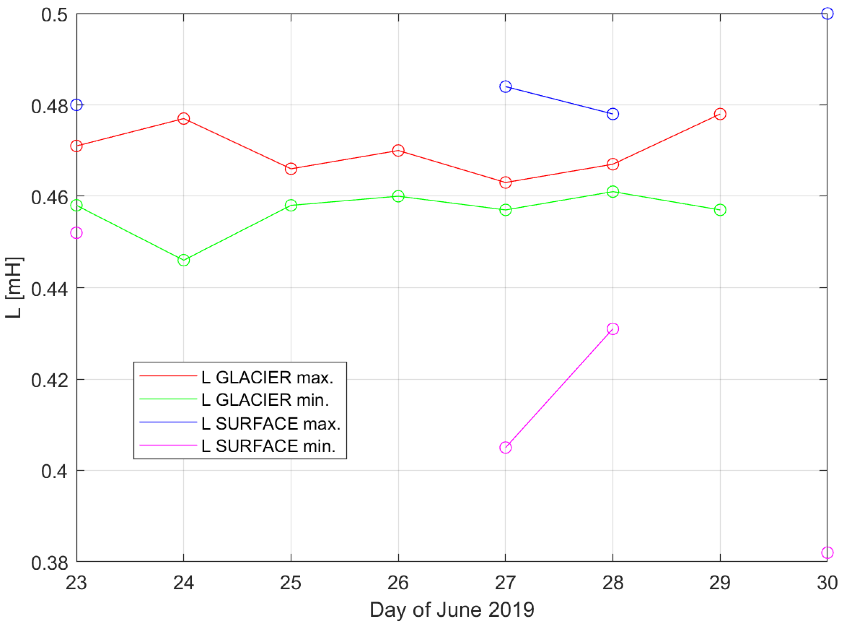
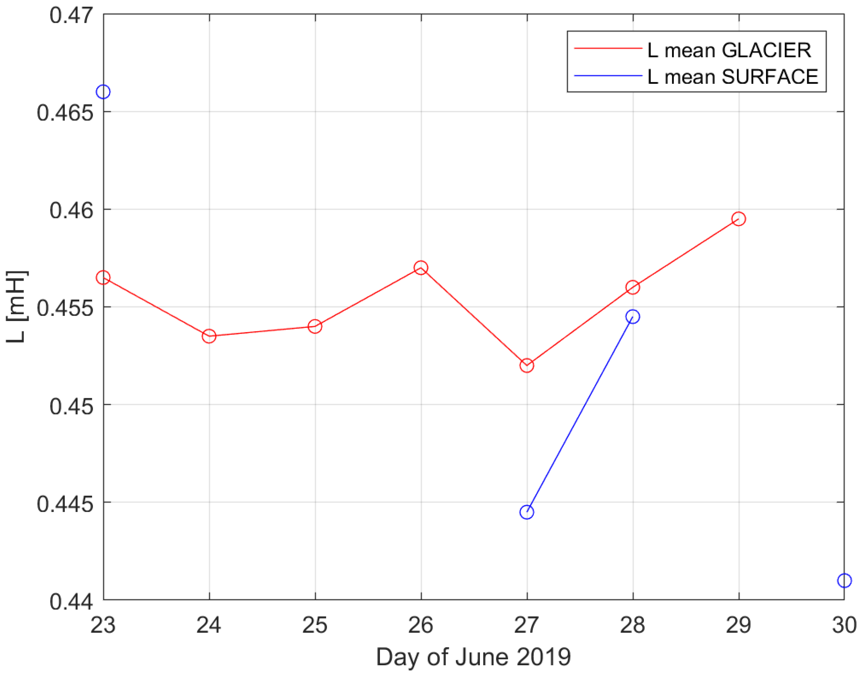
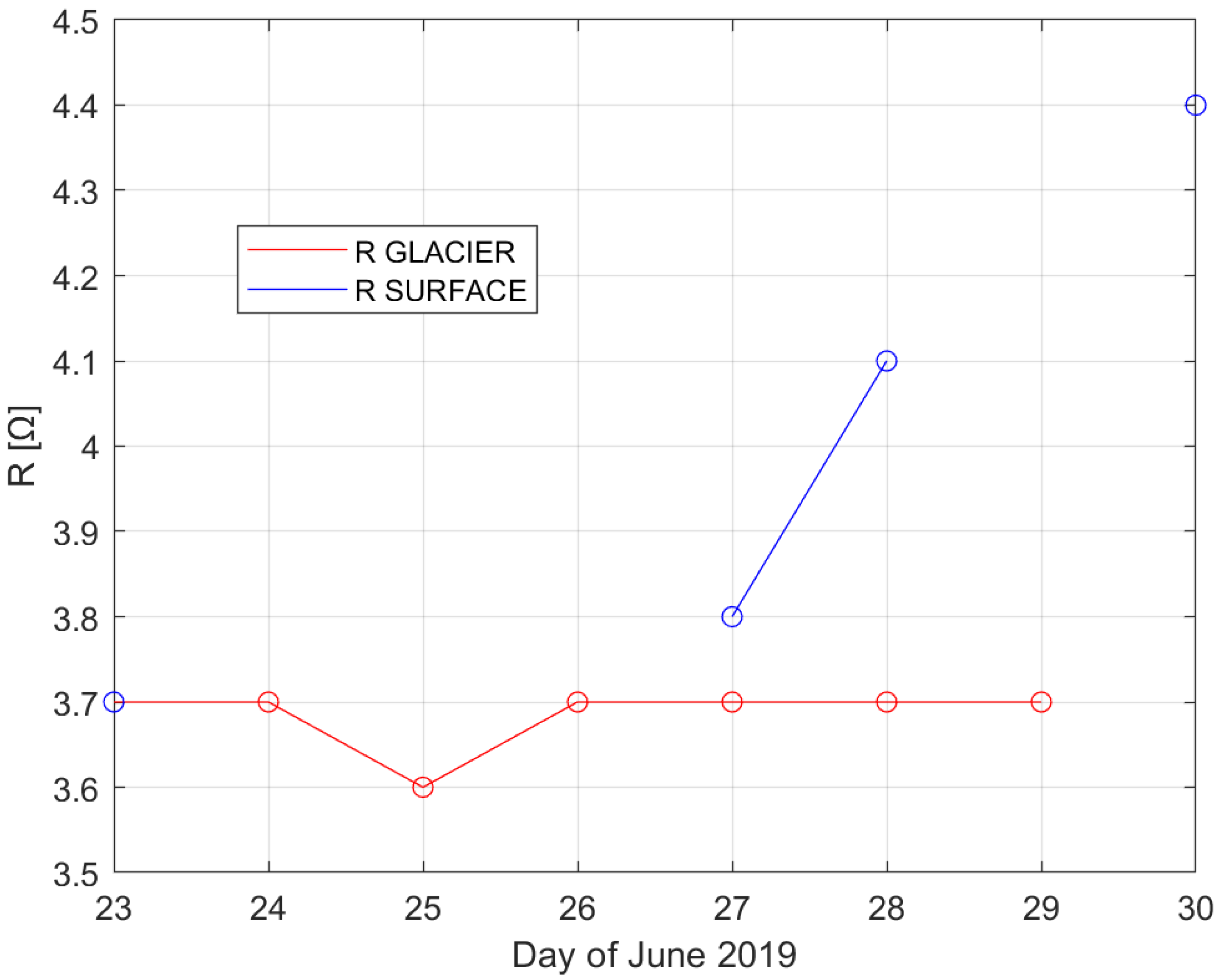
During the operation of the experiment—from 23 to 30 June 2019, with the 30 June as the day when the dismantling of the glacier-based system started, leaving only the surface system operational—every day the inductances and resistances of both antennas were measured. These values, presented on Figure 3, Figure 4 and Figure 5, have been used to calculate the absolute values of the impedances of the antennas and their Q factors for 270 kHz (interpolations by linear functions between the values for adjacent days).

The inductances of both antennas did not remain constant during the measurements-they have varied between the maximal and minimal values, most likely due to changes in the surface features of their ‘cores’ [6]—humans, vehicles, maintenance equipment, other IGLUNA experiments, electrical installations, etc.—the interpolation curves indicate the days when the surface antenna had been damaged by the snowcat’s tracks (as it did not function as a one-loop coil, the inductance could not have been measured).

Despite the fact that both antennas had different shapes and functioned in different conditions (shielded ice cave with approximately constant temperature of −5 °C and no snow versus open space with gravy snow and severe temperature fluctuations, including its daily variations), their averaged inductances converge to a value between 0.45–0.46 mH.

The resistances of the antennas (despite the temperature differences) remained nearly equal, with the value of 3.7 Ω. The first repair of the surface antenna—performed by cable braiding—increased its resistance to 4.1 Ω; the second repair, employing a pair of banana plugs from the already dismantled glacier antenna system, increased the resistance of the antenna to 4.4 Ω. This clearly indicates that despite the fact of extreme (in relation to the Earth’s surface) environmental conditions, the resistances and inductances of such antenna systems are not severely affected and remain mostly unchanged.

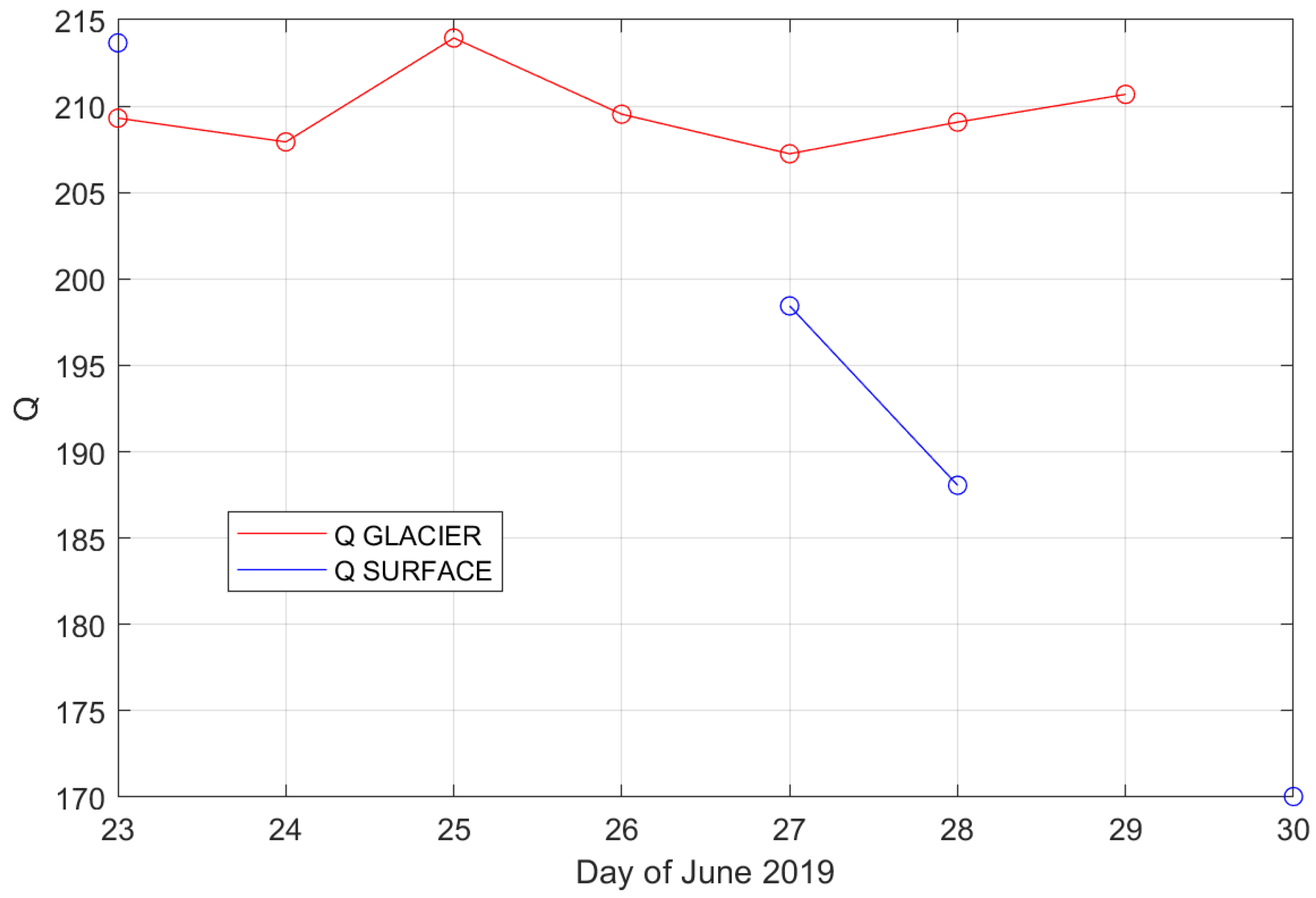
Measured inductances and resistances of both antennas allowed the calculation of the Q factors using a conventional formula for RLC circuit as the inversion of the coefficient describing the damping of the oscillations [13]:

$$Q=\frac{2\pi fL}{R}$$

(1)

where f is the circuit’s operating frequency (Hz); L, inductance (H); and R, resistance (Ω). The approximate impedances Z for the respective days of operation have been calculated using a formula for a series circuit [13], as the deployed antennas operated as RL in-series loops of the transmitters’ drain circuits [7,13]:

$$Z=\sqrt{R^2+4{\pi }^2{f}^2{L}^2}$$

(2)

with the total resistance of the circuit approximated by the dominant DC resistance; the accurate calculation of the total resistance for large and highly irregular loops requires different and much more complex methods than for small loops [10] (including the precise definition of the antenna’s surroundings, which in this case were neither simple nor constant). The calculated Q factor values and approximate impedances for 270 kHz are shown on Figure 6 and Figure 7.

The changes of the Q factor, related to the changes of the inductances, show convergence to the value of ~210 this, when used to calculate the available bandwidth for the A3E type of emissions, gives only bandwidth (BW) = ~1.4 kHz too low value for a recognizable voice/telephony modulation. The actual parameters of the antennas—the DC resistances, inductances and the Q factors, respectively—were affected by the modulation transformers, which became the in-series parts of the antenna circuits, allowing a sufficient increase of the bandwidth obtained during the experiments’ operation to allow sound/voice transmissions (see Section 4).

Both antennas remained as untuned (no external capacitor) high-impedance circuits [4], with approximate impedance values of nearly a half of the input impedance of a high-power longwave transmitter’s power stage [14]: ~773 Ω.

As the antennas possessed the length of quarter-wave values for 270 kHz (278 m), the analytic definition of their radiation resistance becomes complicated, especially with the inclusion of their actual shape after laying down in and on the glacier, and random objects and systems present on the surfaces of their ‘cores’. However, if such antenna is considered to be a singular loop of a flat coil, using the measured inductance values respective specific magnetic permeabilities μ_r of the surrounding medium can be calculated by using the adaptation of the formula given in [15]:

$$L={\mu }_0{\mu }_r\frac{r}{2}{\mathsf{\Psi }}_{zA}$$

(3)

where μ₀ = 4π∙10⁻⁷ H/m (magnetic permeability), r is the radius of the antenna (assuming circular shape: 44.245 m) and Ψ_zA, the magnetization flux (here equal to 20 [15]).

The calculated μ_r values vary in the same way as the inductances and range from 0.835 to 0.880—this indicates a diamagnetic environment, which is consistent with the geological composition of the Alps in this region [16] and a large (yet still smaller than the wavelength) presence of ice. This calculation could be adapted in a system for remote surveying the glacier- and mountain’s state by analyzing the magnetic permeabilities of wire loops laid in different regions and positions.

3. Antennas’ Surroundings the Parameters of the Ice

As the environment surrounding both inside-glacier- and surface antennas would not only play a key role of determining their physical state during exploitation, but also affecting their performance as radiating structures.

For the LF region (30–300 kHz), the electrical permittivity of ice remains constant and is close to the value of 3 [17]. To calculate the tangent of loss angle tgδ for 270 kHz, equal to the conductivity divided by the multiplication of pulsation and the electric permittivity, the in situ conductivity of the Klein Matterhorn ice had to be defined. A series of measurements were performed using two spike probes with their tips recessed in the clean wall of the Glacier Paradise, giving the resistance-in-distance and conductivity-in-distance graphs (Figure 8 and Figure 9; the distance between the probes was the varied parameter).

It can be clearly seen that the changes of both parameters are rapid below the distance of 40 mm. It can be explained as such due to the structure of the ice—despite being the so-called glacier ice, dense and with few intrusions of gases, it remained covered with very thin (atomic) layer of liquid water (which decreased the resistance when the spike probes were close to each other) and crystallized in a non-uniform way—the crystallization seeds’ borders and non-zero amount of gas intrusions most likely played a key role in the increasing of the resistance between the probes above the 40-mm distance between them. Figure 10 presents the calculated tgδ for 270 kHz.

For the closely-located probes, the tgδ value is close to the one defined in [17]: ~0.25; for larger distances it decreases below 0.01, showing that the Klein Matterhorn/Glacier Paradise ice did not pose a significant obstruction for the radiation of 270 kHz by the considered loop antennas.

4. Transmitter Design

The initial transmitter design was based on D-class H-bridge power MOSFET technology, similar to the design used in the Solec Kujawski Radio Transmitting Centre of the Polish Radio Program 1 (225 kHz; [18]). As the change to lower powers had been imposed, a new design was created, based on the C-class controlled carrier/A-class A3E-SC (analog double-sided amplitude-modulated telephony with suppressed carrier) single power MOSFET (ST Microelectronics, Geneva, Switzerland, STW20NK50Z) transmitter [19], enclosed in a low temperature-protective casing, shown on Figure 11.

Each transmitter had its own frequency generator, based on a digital switch operated in astable mode with adjustable RC circuit (adjustable air capacitor) and sockets for spike probes to measure the generated frequency. The bias voltage, changing the characteristic of the power amplifier to provide good linearity for AM, was fed by a set of built-in batteries (a similar battery pack powered the frequency generator). LF modulation signal entered the circuit through a mini-jack plug; the main power for the transmitter was provided by a laboratory power supply, mounted externally. The modulation was realized by a 6-watt modulation transformer. The antenna was coupled in-series to the final stage circuit (no antenna transformer).

Each circuit was placed on a Styrodur base inside a plastic case. On the instrumentation panel three indicators were placed: to monitor the frequency generator voltage (as the digital switch could stop operating if the voltage dropped), the gate bias voltage and the transistor’s temperature measured on the drain’s heat sink. As the circuit board protruded outside the transmitter box, it was equipped with two different shields against the outside temperatures and mechanical shocks: industrial casted glass dome (meant for the Glacier Paradise transmitter) and an original Thermos tin box (meant for the surface transmitter). Both transmitters in operation are pictured on Figure 12.

The on-site modulation control (by direct reception and demodulation) of the emitted AM signals on site was carried out using three types of mobile radio receivers, equipped with ferrite antennas for the LW range and tilted to comply with the transmitting antennas’ polarization: Unitra Dana MOT 728-2 [20], Eltra Jowita 2 [21] and KUPZ/Tento Neywa 402 [22], with Jowita 2 proving best due to its high selectivity and sensitivity. Both Dana and Jowita were equipped with acoustic (after-demodulation) interfaces to microcontrollers of the 2.4-GHz system to collect telemetry and sensor data.

5. Transmission Performance Comparison of Propagation Models

5.1. Long-Range Receptions

Every day marked by the functional loop antennas, after applicable transmitter and antenna checks [23], the system went into operation. The basic goal of it was the communication channel through the ice ceiling of the Glacier Paradise, enabling the sending of data/telemetry between the simulated lunar habitat and the surface EVA (extravehicular) team. The emitted signals would be picked up by the receivers mentioned before (with Neywa being the smallest one–most convenient for the EVA activities).

During the initial runs of the system the quality of the signal in the glacier remained satisfactory and clear; in the later days the LW frequency band has become cluttered with industrial emissions, generated by the PWM controllers as well as the maintenance- and construction equipment, rendering the Klein Matterhorn 270 kHz reception impossible (except for a single ‘sweet spot’ on the surface of the glacier, however impractical for the EVA activities).

To rectify the problem, the operation of the entire experiment was modified; the 2.4-GHz surface system operated independently from the habitat, and the longwave system tests aimed at long-range reception outside Klein Matterhorn (without any changes to the previously defined transmitters’ power). Experimentally, two transmitters were coupled to the same antenna, operating on 270 kHz as the main frequency for A3E-SC telephony (acoustic signal, classical music) and on 266/274 kHz subcarrier with P1A (narrow-bandwidth amplitude-modulated impulses) telemetry—the frequencies were chosen in a way that both emissions reside in the broadcasting bandwidth of 9 kHz, not interfering with adjacent LW broadcasts. To achieve the long-range reception, a wide group of LW listeners was mobilized via social media to monitor the LW bandwidth outside the range of RKS Topolná.

The signal was successfully received more than once; the farthest and best quality recording came from Finland at the location of KP20JO [7]. The transmissions were received to the north of Helsinki at 60.6°N 24.8°E, making the distance of 2077.06 km from Klein Matterhorn (see Figure 13), with the transmitter located at 3868 m a.s.l. and the receiver at 27 m a.s.l.

With the receiver’s noise at 0.010 μV/m, the A3E-SC signal was recorded at approximately 0.016 μV/m and the P1A at approximately 50 μV/m—values making the signal barely detectable for ordinary commercial LW broadcasting receivers (specialized equipment needed), yet still surpassing in this location its stronger but low-land counterpart of RKS Topolná by nearly 775 × 10³ times for the E field intensity of the carrier and nearly 500 times for the E field intensity of the sidebands [8].

Comparing the obtained results (maximum range and frequencies employed) with the formulas given by Watt [24] for the angle of arrival of the radio wave travelling along the surface of the earth for a given range, the approximate angle of arrival reaches ~1 degree—which may indicate that the wave propagated directly, without multiple reflections from the ionosphere or ground surfaces.

5.2. Proposed Propagation Models

Frequencies used for these transmissions belong to the upper part of the low frequency band (30–300 kHz), designated internationally for longwave (LW) radio broadcasting services. The propagation of these frequencies can be described by many formulas [25,26,27], among which the purely theoretical ones possess significant amounts of inaccuracies and remain barely useful for practical implementations [26]. The solution to these issues is the choice of formulas based on long-lasting experimental research on the RF propagation and reception, which include the natural (and difficult in simulation) characteristics of the terrestrial propagation environment. Such formulas had been formed by many researchers and institutions–including the CCIR (Comité Consultatif International des Radiocommunications, currently ITU-R) [28] and EBU (European Broadcasting Union, also UER-Unión Europea de Radiodifusión) [29].

The CCIR had issued a series of graphs with curves describing the E field intensity (RMS) in relation to the distance for ground wave and ground properties as parameters (conductivity and specific electric permeability) [28]. From the graph depicting curves for the conductivity of 1 mS/m and ε_r = 4 (the closest values to those calculated above), an interesting property can be read—the actually-achieved maximal distance is described by the curve belonging to the frequency nearly twice lower (2000 km for 150 kHz, versus 1000 km for 300 kHz).

The UER ground wave formula (but for vertical antenna), used to calculate approximate E field strength (RMS) in the LW broadcasting range, is presented as follows [28]:

$$E \left[\frac{mV}{m}\right]= \frac{300r^2\sqrt{P_{\mathsf{\Sigma }}G}}{{\left(r^2+4Z_{eff.}^2\right)}^{\frac{3}{2}}}$$

(4)

$$Z_{eff.}=a\left[\frac{\sin \left(\frac{r}{2a}+{\phi }_0\right)}{\sin {\phi }_0}-1\right]$$

(5)

where r is the distance (km), P_Σ is the radiated power (kW), in this case: 0.000426 kW (A-class A3E-SC), G is the antenna gain (here assumed 1), Z_eff. is the effective height of the reflective layer of the ionosphere, a is the mean Earth’s radius (6378.14 km), and φ₀ is the angle of incidence on the ground wave on the reflective layer of the ionosphere, estimated using [28] at 82.16°.

For the ionospheric wave (emitted by a vertical antenna at night hours with the middle of the distance experiencing midnight at local time, magnetic declination of 61° and Wolf number equal to 0), the UER gives the following empirical formula [28]:

$$E\left[\frac{\mu V}{m}\right]=\frac{10233}{\sqrt{r}}\sqrt{P_{\mathsf{\Sigma }}G}\cdot e^{-8.94\cdot {10}^{-4}}{\lambda }^{-0.26}r$$

(6)

with λ being the transmitted wavelength [km].

As the performed experiments were carried out in an untypical setting for a longwave broadcasting–vertical loop antenna, nearly 4 km above sea level, diamagnetic surroundings, singular obstacles on the signal’s way, very low power–formulas describing the propagation of surrounding frequency bands are also considered for comparison, regardless of their constraints (the same rule was applied for the formulas mentioned above). Four such formulas were taken into consideration.

The Austin–Cohen formula [28,29] is often used to calculate the E field intensity in the VLF and lower LF frequency ranges, with the leading influence of the ionospheric wave; best applicable for sea-dominated distances. The formula is given as:

$$E\left[\frac{mV}{m}\right]=\frac{300}{r}\sqrt{P_{\mathsf{\Sigma }}G}\sqrt{\frac{\alpha }{\sin \alpha }}{e}^{-\frac{0.0014r}{{\lambda }^{0.6}}}$$

(7)

with α being the central angle (angle measured on the planet’s great circle) between the transmission and reception points; here equal to 18.66°.

For the region adjacent to LF, the VLW/VLF (very long wave/very low frequency), the following formula was proposed in [28] (approximate; for planetary waveguide propagation):

$$E\left[\frac{mV}{m}\right]=\frac{245\sqrt{P_{\mathsf{\Sigma }}G}}{\sqrt{\left(a+\frac{Z_{eff.}}{2}\right)Z_{eff.}\sin \alpha }}$$

(8)

with Z_eff. calculated using Equation (5).

As the performed experiments used a great advantage of the transmitter’s elevation above the sea level to achieve a large distance, a formula incorporating this mechanism could be taken into consideration—a formula by B. A. Vviedenskiy [28] (for the UHF range):

$$E \left[\frac{mV}{m}\right]=\frac{2.18\sqrt{P_{\mathsf{\Sigma }}G}{h}_1{h}_2}{r^2\lambda }$$

(9)

where h₁ and h₂ are the heights of transmitting and receiving antenna positions [m], here 3868 and 27 m, respectively. This formula is to provide best results for h₁h₂ ≤ r[m]∙λ/18 (in this case: h₁h₂ = 104,436 m² < rλ/18 ≈ 128 × 10⁶ m².

The last formula (the ‘diffractive’ formula) allows to calculate the E field strength slightly farther than in the visual distance r_H (best for r_H < 8.24∙(h₁^0.5 + h₂^0.5)) and is approximately described as [28]:

$$E\left[\frac{mV}{m}\right]= \frac{4.25\sqrt{P_{\mathsf{\Sigma }}G}{h}_1{h}_2{r}_H^{n_t-2}}{r^{n_t}}$$

(10)

where n_t is the indicator of attenuation of the radio wave behind the horizon–defined for LW as close to 2.5 [28].

Equations (4)–(10) have been plotted altogether for a comparison of their results (Figure 14 and Figure 15).

The diffractive formula gave results the closest to the ones achieved by P1A emission on 266 kHz, yet the course of this function remains far from expected values; B. A. Vviedenskiy’s formula gave too low values. The ground wave formula by the UER (best fitting for the frequencies used in the experiment), the Austin–Cohen formula and the VLW formula (long-range low frequency communication) appear best for adaptation to approximately describe the propagation of A3E-SC and P1A/CW (continuous wave) emissions, respectively, with the given constraints:

• 140–150 times higher elevation of the transmitting antenna in relation to the receiving antenna;
• upper part of the LF frequency band;
• horizontal quarter-wavelength singular loop transmitting antenna; and
• antenna positioned in a diamagnetic structure.

The re-formulation of the Austin–Cohen formula (Equation (5)) requires its division by 10 to describe the E field strength at A3E-SC at large distances; if the VLW is multiplied by 3.33, it could be used to describe the E field strength for P1A at large distances. The re-formulation of Equation (2) requires the development of a coefficient which includes the height square root sum, mentioned above in the description of Equation (8). Assuming that this coefficient would take the following approximate form (for its parameter values given above, it would put approximately equal the results of Equation (2) to the experiment’s results):

$$n_e\left(h_1,h_2, r\right)=52.4\cdot {10}^{-4}\frac{\sqrt{h_1}+\sqrt{h_w}}{r}$$

(11)

Equation (4) would be reformed into (Equation (5) remains unchanged):

$$E^{\prime }\left[\frac{mV}{m}\right]=1.573\cdot {10}^8\sqrt{P_{\mathsf{\Sigma }}G}\frac{r\left(\sqrt{h_1}+\sqrt{h_2}\right)}{{\left(r^2+4Z_{eff.}^2\right)}^{\frac{3}{2}}}$$

(12)

The accuracy and utility of these formulas for determining the E field strength distribution for this transmission case are to be verified in the next planned experiments—as the effects of the comparison and the reformulations are based on the signal data at maximum distance with few data on shorter distances (this verification would give an insight on the E field strengths on shorter distances—which formula in terms of its course is best applicable for the achieved results).

6. Communication Channel Analysis

The simultaneous registration of the P1A (maximized concentration of RF energy in the transmission [4], similar to plasmasphere-aiming test transmissions [30]) and A3E-SC emissions on the maximum range location allowed the description of the received electric field value as a function of the signal’s bandwidth B_UA (signals from the under-ice antenna) and the calculation of the channel capacity C [bit/s] as a function of the signal’s bandwidth [31]. Figure 16 presents the latter function plotted. It can be clearly seen that this type of communication channel does have a maximum available capacity at approximately 2.5 kHz of 15.5 kbit/s. This capacity shows that the system, despite its limitations (very low power, inconvenient polarization), already complies with the requirements for the bit rates needed by the modes A and B of the DRM30 digital modulation system [32]–if the bandwidth could be increased to min. 4.5 kHz (i.e., by an additional non-linear component).

The bit error rate (BER) for the deployed system has been analyzed as a function of the net bitrate [8] for two bandwidths: 2.5 kHz (maximum from Figure 16) and 4.5 kHz (minimum for the employment of the ‘Digitale Radio Mondiale below 30 MHz’ standard–the DRM30 [32]). Considering the net bitrate equal to the available channel capacity, for 2.5 kHz and 15.5 kbit/s (from Figure 15) the BER value is 0.2362; for 4.5 kHz and 7 kbit/s, the BER drops to 0.0757 [8]. Both these values remain too high for a successful implementation of the DRM30, as the minimum BER described as the ‘limit of service’ is equal to 10⁻⁴ [32]. This issue can be rectified by the increase of the SNR—the increase of the transmitting power.

7. Conclusions

For the first edition of the IGLUNA program a means of direct communication between an ice-cave-hidden lunar habitat and the surface was proposed. This system, operating on longwave of 270 kHz with possible subcarriers (in the broadcasting part of the spectrum with magnetic quarter-wavelength loop antennas on high altitude), was set up and operated in June 2019 on the Klein Matterhorn glacier in Switzerland. Basic measured and calculated parameters of the antenna system were presented; a formula describing the obtained field intensity versus distance has been proposed. The parameters of the surrounding medium have also been measured and calculated. The system showed a possibility of radio communication on large distances, as well as a possibility of remote longwave sensing of the nearby rock and ice layers [4], similar to ground penetrating radars [33,34,35]-applicable also on the IGLUNA program’s targeted celestial body, where the attenuation of the signal is expected to be even lower due to less lossy environment than on humid Earth [36].