1. Introduction
Since 1998, the International GNSS Service (IGS) Ionosphere Working Group (IONO WG) has been continuously releasing global maps of the vertical total electron content (VTEC) in their rapid, final, and predicted schedules. The IGS Ionosphere Combination and Validation Center (ICVC) at University of Warmia and Mazury is responsible for the ensemble analysis of the global VTEC maps synthesized independently by several IGS Associate Analysis Centres. ICVC computes its combined “weather” VTEC map by weighing provided input VTEC values according to the observation uncertainty metrics that were determined by collective validation of computed VTEC against the original slant TEC (STEC) measurements [
1].
Contrasting the ICVC-released weather VTEC maps to their quiet-time counterpart (i.e., climate) is a powerful instrument in space physicist toolbox: such
weather-minus-climate deviation maps allow rapid assessment of the near-space plasma dynamics as it responses to a wide variety of impacts in the Sun-Earth system, ranging from the forces acting in the outer space to the processes on the surface and even underneath the Earth’s crust. However, development of such global quiet-time VTEC reference maps proved to be a difficult task, given the staggering complexity and dynamics of the constituent subsystems and their couplings (see: [
2,
3]). Our approach to the task of building the quiet-time reference for the weather-minus-climate deviation maps is to compute daily empirical 30-day running average VTEC. Such averaging is expected to filter out the effects attributed to ongoing activities in the near-Earth environment that would otherwise distort presentation of the ionospheric/plasmaspheric climate. At the same time, the 30-day averaging would still capture the annual cycle specifics that are important for the weather-minus-climate analysis.
We have incorporated the global 30-day average empirical TEC mapping capability into the GAMBIT service [
4] operated by GIRO (Global Ionospheric Radio Observatory) [
5]. GIRO provides measurements recorded by ionosondes, the high frequency ionospheric sounders known for their original contributions during the International Geophysical Year 1957-1958 and during the follow-on decade to the global empirical plasma density models for IRI (International Reference Ionosphere) (see: [
6,
7] and references therein). Since that time, when the Committee on Space Research (COSPAR) and the International Union of Radio Science (URSI) recognized the need for an international standard ionosphere and formed an Inter-Union Working Group to develop it, IRI has evolved into one of the most successful and widely used ionospheric models, recognized as the official standard for the ionosphere by the International Standardization Organization (ISO). The IRI design has been rooted in the concept of capturing the experimental evidence, as measured by variety of sensors on the ground and in space, without relying on the evolving theoretical understanding of the underlying geospace processes in their complex interaction. After its success of representing the quiet-time climatology of the ionosphere, IRI has more recently included several options to describe typical storm-time plasma dynamics as well.
Given the high IRI ratings reported in comparisons to other density models of the ionosphere (see: [
8,
9,
10,
11,
12]), including those with data assimilation capability, the IRI science team formed a task force to develop
real-time assimilative IRI extensions [
13] so as to further improve its performance in the nowcast mode. RION operates one of such nowcast services, "IRTAM" (IRI-based Real-time Assimilative Model) [
14,
15]. Every 15 min, IRTAM computes and publishes global ionospheric “weather” maps of four parameters for the IRI bottomside density profile description: peak density NmF2, peak height hmF2, and the standard IRI bottomside profile shape controls, B0 and B1 [
7]. Global weather-minus-climate deviation maps are then computed and disseminated via Global Assimilative Model of Bottomside Ionosphere Timeline (GAMBIT) Database and Explorer [
16] for public online access (see:
http://giro.uml.edu/GAMBIT/).
Following the recommendations of the International Reference Ionosphere (IRI) Workshop 2017 in Taoyuan City, Taiwan and International GNSS Service (IGS) Workshop 2018 in Wuhan, China [
17], we present results from a new global ionosphere mapping system that fuses data from two separate sensor networks: IGS permanent GNSS receivers providing VTEC measurements and GIRO ionosondes providing data for RION weather nowcast. The system is capable of reproducing the equivalent slab thickness τ [
18] as soon as IGS and GIRO measurements become available, thus expanding the capabilities of GAMBIT database and explorer system: the ionospheric slab thickness dynamically responds to changes of the neutral gas temperature and the
transition height [
18], supplementing the ionosonde-derived bottomside specifications with descriptions of the ionospheric profile above the F2 layer peak. The slab thickness τ is defined as a ratio of the vertical total electron content in TEC units (electrons per square meter) to the F2 layer peak electron density (NmF2) in electrons per cubic meter. The slab thickness (expressed in meters) is an important parameter of an imaginary ionosphere that has the same TEC as the actual ionosphere and constant uniform density equal to NmF2 and represents its vertical extent.
The main motivation of the research was to establish data sources and fusion methodology for the joined purpose of throughout ionosphere mapping. It has been done with inclusion of over 10 years of climate VTEC maps to GAMBIT Database and Explorer, which allows fusion with the IRI model and GIRO products. Introduction of climate VTEC maps allowed for computation of climate slab thickness. Further extension of cooperation is planned, including weather VTEC based on rapid products of IGS IONO WG IAACS and-in the future near-real time VTEC.
2. Materials and Methods
2.1. IGS IONO Working Group and VTEC Maps
The IGS Ionosphere Working Group provides scientific and operational oversight of the systems for reliable global VTEC weather nowcast and forecast (see: [
19,
20,
21]). Similarly to other established IGS Working Groups that ensure quality and reliability of GNSS data (e.g., satellite orbits and clocks), IONO WG operates an Ionosphere Combination Center that collects incoming VTEC data from associated VTEC analysis centers for ranking and combining multiple individual values into a single map [
22]. At this time IONO WG continuously releases several well-recognized products of proven quality, with worldwide base of users, containing VTEC maps released in three schedules (
Table 1), as well as ROTI (Rate Of TEC Index) maps depicting ionospheric irregularities over the northern hemisphere [
23].
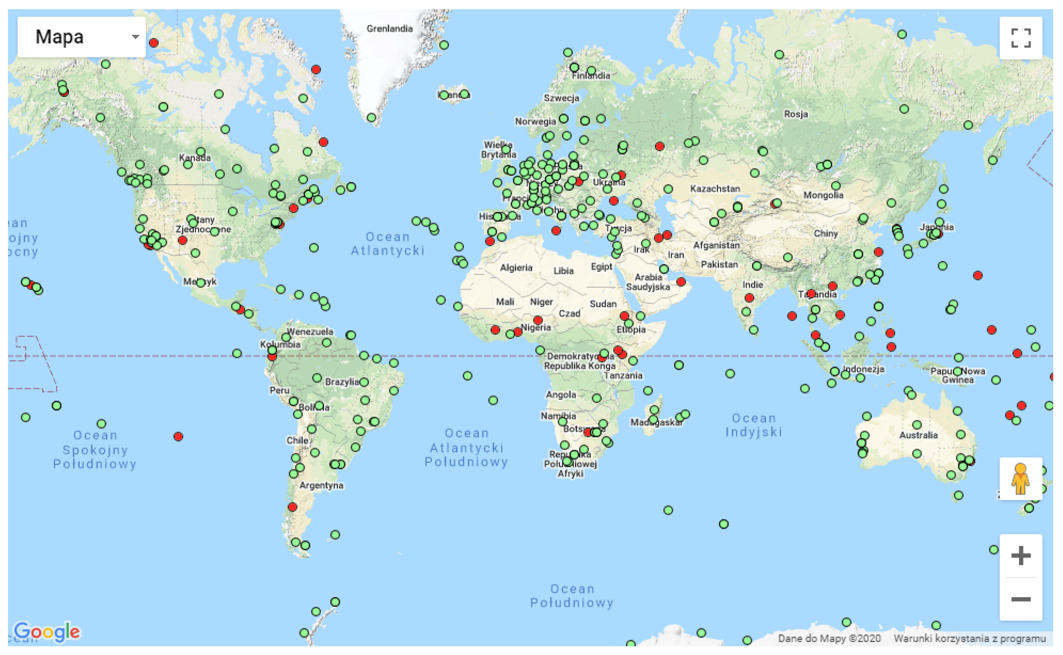
Apart from the official IGS IONO WG products shown in
Table 1, based on GNSS observations from IGS permanent network (
Figure 1), several IGS Ionosphere Associate Analysis Centers (IAACs) such as UPC, CAS and DGFI produce Global Ionosphere Maps (GIMs) in Rapid schedule with increased time resolution of just 15 min. Additionally, there are currently works underway on a combined real-time GIM product based on UPC, CAS and CNES (Centre National d’Études Spatiales) products ([
24,
25,
26]).
In case of IGS IONO WG, all its (and contributing IAACs) products are published at NASA Crustal Dynamics Data Information System (CDDIS) ftp server in dedicated directory
ftp://cddis.nasa.gov/gnss/products/ionex/. To access a specific VTEC product the directory should be appended with elements described in
Table 2 and
Table 3:
Typically, VTEC determination from GNSS observations follow the procedure described by [
27], defining TEC as an integral of electron densities along the line-of-sight between a satellite and receiver in a cylinder with one square meter cross-section:
where
is the electron density along the ray path.
E is TEC value expressed in TECu-TEC Unit equal to
electrons per square meter. In terms of actual GNSS observations, several approaches can be applied, differring in details, but in most general form possible to express as [
28]:
where
is a computed slant TEC value,
c denotes the speed of light in vacuum,
is a time delay between arrivals of signals on two frequencies
and
to the dual-frequency receiver. Such slant TEC can then be mapped on a single-thin-layer ionosphere using mapping formula, such as given by [
29]:
where VTEC is vertical TEC at IPP (Ionosphere Pierce Point-a cross-section of ionosphere thin layer and ray path), STEC is slant TEC,
is the radius of the Earth and
is a height of ionosphere layer over the surface of the Earth.
For this task the UQRG iononospheric maps produced by Ionosperic Associate Analysis Center at Universitat Politecnica de Catalunya in Barcelona, Spain were used [
30], due to their matching 15 min cadence to IRTAM (IRI-based Real-time Assimilative Model) and we work on inclusion of other 15 min GIMs. UQRG maps are produced using tomography model of ionosphere, described in detail by [
31,
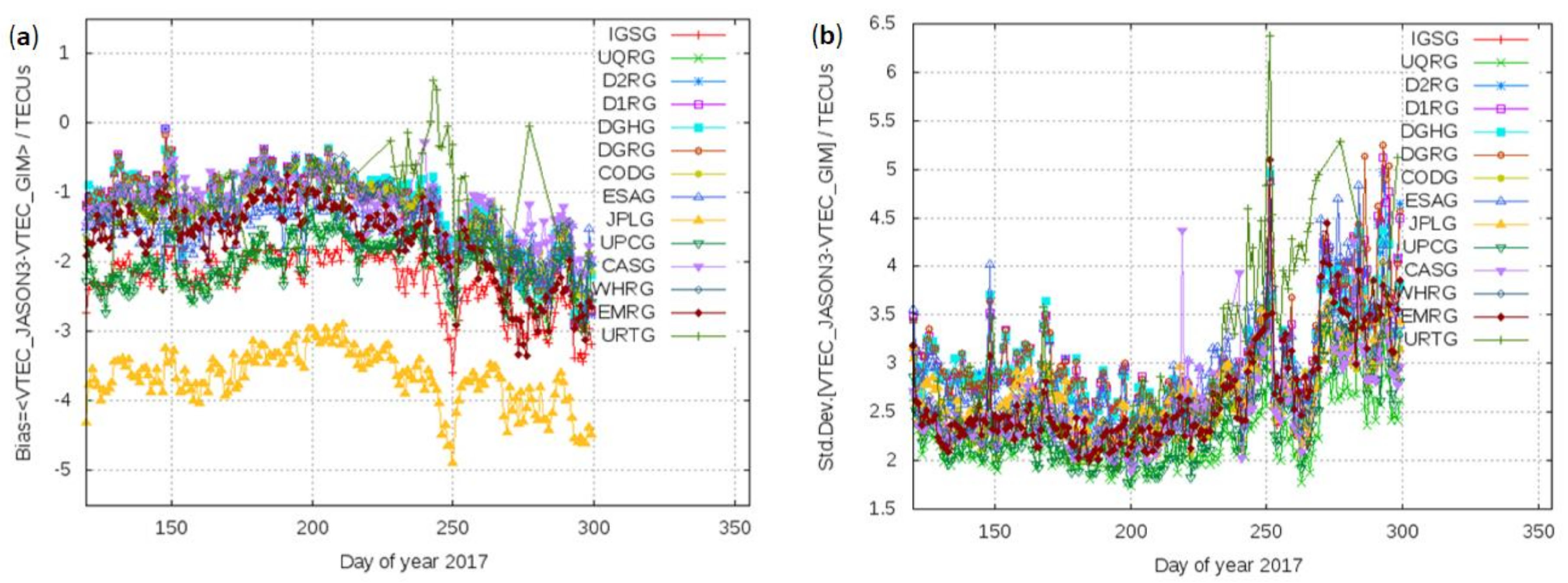
32]. Comparison studies have shown its reliability and quality versus other IGS IAAC-released VTEC products. This can be seen in particular in left plot of
Figure 2, where the daily bias of the difference between the VTEC directly measured by the JASON3 altimeter (up to about 1300 km height and far from stations-over the oceans) minus the VTEC provided by different GIMs in IGS is represented for the most part of 2017.
On the one hand it can be seen that almost all the GIM VTEC biases regarding JASON3 VTEC are in agreement between them at 1 TECU level. This result is in full agreement with the assessment results vs. dSTEC, a more accurate reference, and in the challenging scenario of islands (see in [
33] the right hand plots of Figures 8 and 9).
The well known exception is JPLG which is likely related with the usage of a different mapping function that the common one used by the other IGS centers to build their GIMs.
On the other hand the discrepancy of the GIMs vs. JASON3 are due to an instrumental calibration bias of the altimeter [
34] and to the variability of the topside electron content between the heights of altimeter and GNSS satellites (since 1300 km to 20000 km approximately, see for instance in [
1] Figure 12 and associated comments).
Moreover, in the right hand plot of
Figure 2, the corresponding daily RMS is represented, which time evolution is mostly due to the bias evolution previously commented. It can be seen there the systematic better behaviour of the UQRG GIM (green crosses) selected for this study, regarding other GIMs, which has been confirmed in extended studies [
25]. The performance of UQRG GIM is based on the synergistic application of ionospheric tomography [
31] and Kriging interpolation [
30], without the assumption of a fixed ionospheric height layer to derive the STEC. Of course the common IGS mapping function (
= 450 km in Equation (
3)) is used to transform the STEC in VTEC to build the UQRG GIM in a consistent way for IGS users, which wish to recover accurate STEC values, in particular not far away from the stations used to build the GIM.
2.2. IRI and Data Assimilation
The International Reference Ionosphere (IRI) is an international project that was initiated by the Committee on Space Research (COSPAR) and the International Union of Radio Science (URSI) with the goal of establishing a standard representation of the plasma parameters in Earth’s ionosphere. Such ionosphere model is important for applications that rely on electromagnetic waves traveling through the ionosphere including telecommunication, GNSS, earth observation from space (e.g., satellite altimetry), radio astronomy and many more, because all of these applications need to correct for the retarding and refractive effect of the ionosphere on the probing signal [
36].
IRI’s performance in comparison to ionosphere state derived from GNSS, LEO satellites, incoherent scatter radars, etc. is an object of study since its very beginning, in great details, amongst many others, described by [
37,
38,
39], proving its qualities and helping the IRI becoming the internationally recommended empirical model.
Among other changes, the most recent IRI-2016 [
6] introduced two new models for the F2 peak electron density height, hmF2, and improvements of the ion composition at low and high solar activity. Additionally, a number of changes were made regarding the input and use of solar and ionospheric indices, and some performance improvements were made to the program code (FORTRAN) to speedup the computation of IRI values, which is available both via web-based interface and as a standalone application.
The standard IRI model describes average conditions quite well and has shown excellent results in comparisons with other models [
8,
9,
10,
11,
12], however its performance can be even more improved if observations are available for a time of interest in real-time or retrospective. IRI lets a user provide measurements for the E, F1, and F2 peak density (or plasma frequency) and height and the whole profile is then adjusted to these input parameters. Another simple method is by way of an ionospheric-effective solar index that is obtained by adjusting IRI predictions to either ionosonde measurements [
40], or GPS Total Electron Content (TEC) maps [
41], or GPS slant TEC data [
42]. This approach has been recently further developed by [
43,
44,
45], leading to the IRI-UP version of the model. The IRI Real-Time Assimilative Mapping (IRTAM) of [
14] is based on plasma frequency (foF2) measurements by the worldwide network of Digisonde stations (the Global Ionospheric Radio Observatory (GIRO)) and employs a linear optimization technique to obtain an improved global representation of foF2 for IRI every 15 min. [
46] explained in great details combination of ionosonde and GPS data, main advantage of which turned out to be the possibility of solving the vertical structure of electron density of the ionosphere, which can be described with slab thickness.
Implementation of climate TEC data into GAMBIT database allows its combination with IRI and GIRO data and will contribute for establishing the conditions and methodology for full climate and weather TEC implementation into real-time IRI.
2.3. NmF2-GIRO and GAMBIT
The Lowell GIRO Data Center (LGDC) implements a suite of technologies for post-processing, modeling, analysis, and dissemination of the acquired and derived data products that form the basis of the RION nowcast:
IRTAM 3D, the real-time assimilative model released periodically in form of the “global weather” bottomside ionosphere 2D maps of the IRI-compatible profile parameters, as well as the weather-minus-climate deviation maps from the quiet-time IRI reference;
GAMBIT Database and Explorer with access to 15-minute IRTAM maps since 2000;
40 million ionogram-derived records of URSI-standard ionospheric characteristics and vertical profiles of electron density;
10+ million records of the Doppler Skymaps for evaluation of irregular plasma structures and bulk velocity drift over the GIRO locations;
Digisonde-to-digisonde measurements for detection and evaluation of Traveling Ionospheric Disturbance (TID); and
HR2006 ray tracing system [
47] mated to GAMBIT database.
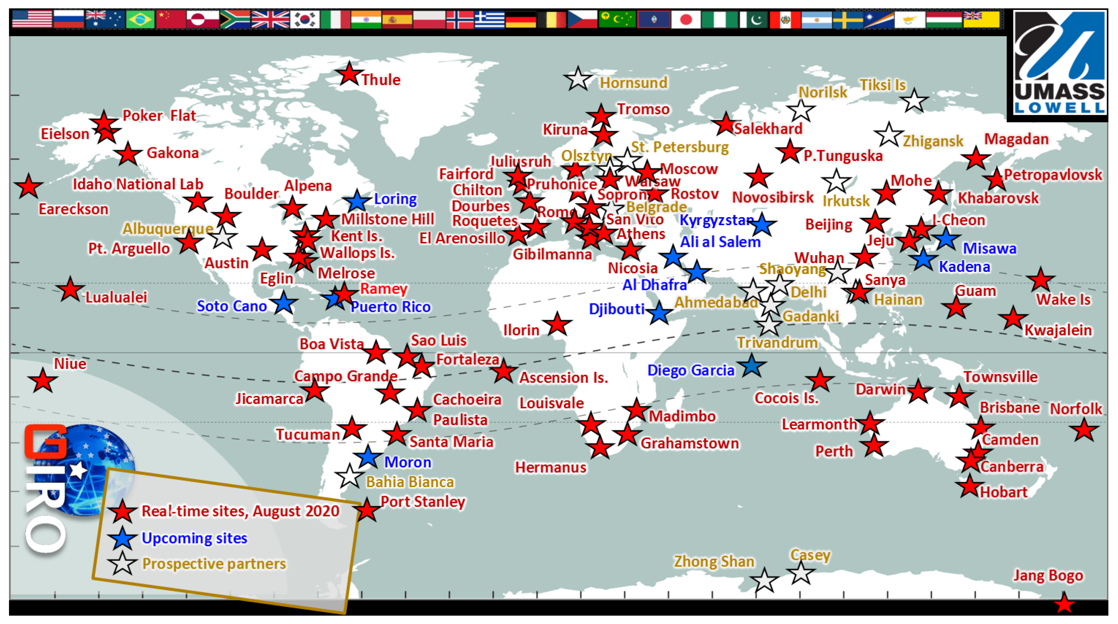
In cooperation with the URSI Ionosonde Network Advisory Group (INAG), LGDC has established cooperative agreements with ionosonde observatories in 30 countries to accept and process real-time data of HF radio monitoring of the ionosphere, and to promote a variety of investigations that benefit from the global-scale, prompt, detailed, and accurate descriptions of the ionospheric variability (
http://giro.uml.edu/).
Currently GIRO network includes ~60 online ionosondes (see: [
5,
48]) shown in the
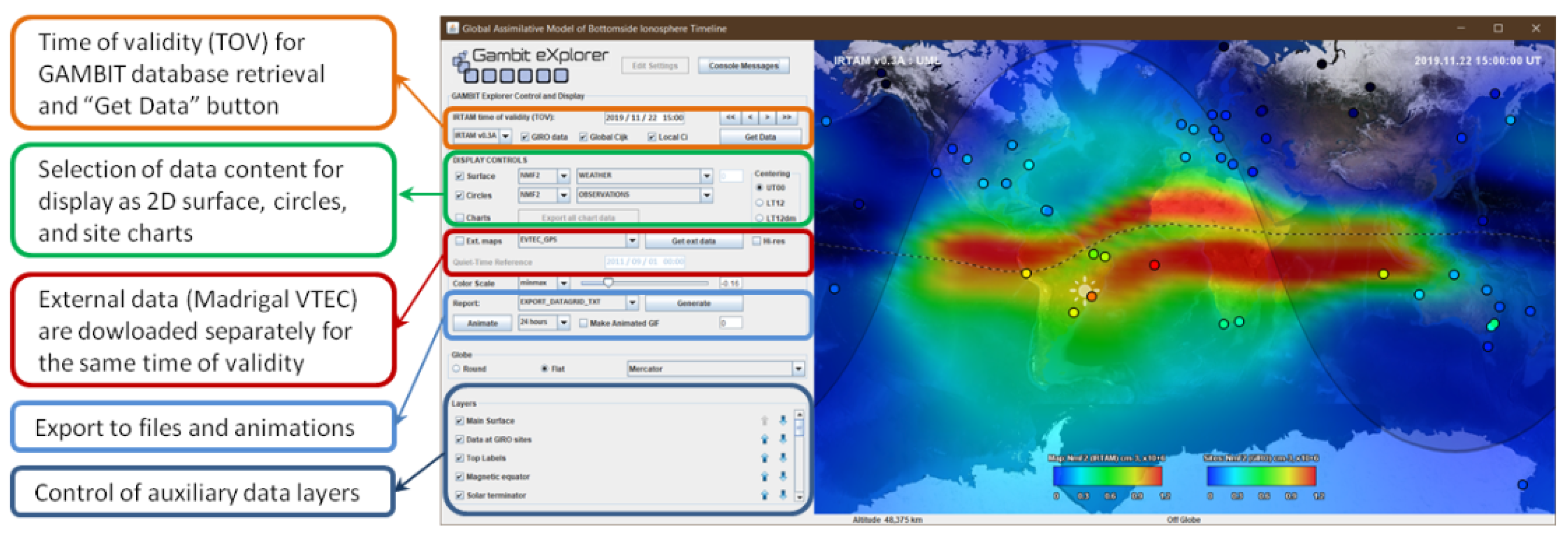
Figure 3 that deliver, among other data products, the maximum electron density at F2 layer peak (NmF2) at each ionosonde location. Global maps of NmF2 are available in GAMBIT database with an interactive access via GAMBIT software (
Figure 4). GAMBIT Explorer is a Java application based on NASA WorldWind graphics library, released for academic research use at
http://giro.uml.edu/GAMBIT, which allows for rapid and interactive visualisation of different ionospheric properties, such as F0F2, NmF2, HmF2, B0 or B1 in various routines (interpolated climate and weather or observations at GIRO sites). But most importantly it integrates different data sources and allows for their combination in a goal of delivering a detailed insight in the ionosphere. Detailed description of the GAMBIT database and Explorer, as well as underlying formalism and algorithms can be found in [
16]. Incorporation of the climate global VTEC maps (described further) led us to extend the capabilities of GAMBIT Database in the climate aspect and opened the path for planned inclusion of weather VTEC.
We will focus on one observed property of the ionosphere in the RION data product roster: peak electron density in the F2 region, NmF2. As most ionized and most dynamically changing region of the ionosphere, F2 displays strong variability depending on the season, time of day, geographical location and level of solar activity. Maximum daytime electron density NmF2 is usually observed one hour after local noon, for mid-latitude locations, and at the altitude of about 300 km [
49], reaching up to
electrons per cubic centimeter, el/
. RION provides NmF2 data derived from the ordinary-wave critical frequency of the F2 layer (foF2) observed by GIRO ionosondes, using the following expression [
50]:
NmF2 is an important physical quantity for space weather forecasts or radio communication, and thus precise observation and accurate analysis are essential [
51].
A quite novel addiction to GIRO capabilities is a methodology of real-time TID tracking using ionosonde data, which is an example of a huge potential still lying in this network [
52,
53].
2.4. Global Climate VTEC Maps
Following the IRI Workshop 2017 and IGS Workshop 2018 recommendations [
17], based on the UPC UQRG VTEC maps, the climate VTEC maps were created using 30-days moving average for each epoch and coordinates. For each epoch (15 min interval, resulting in 97 epochs per day) climate VTEC (overlined) for each cell is computed using formula:
where
is an climate VTEC value computed for each epoch (
e), latitude (
) and longitude (
), averaged over 30 preceeding day series of VTEC values for the same time of day (e.g., 8:15 UT), latitude and longitude and
means the day for which the climate prediction is prepared.
Resampling is then conducted for compatibility with GAMBIT Explorer internal data grid management. Resulting averaged climate VTEC map is remapped from original 2.5 degrees lat and 5 degrees lon to NASA WorldWind 4 degrees lat and 8 degrees lon using efficient natural interpolation algorithm described by [
29]:
where
is the value of the interpolated point
x,
M is the number of natural neighbours (i.e., number of Voronoi cell edges),
is the value of the
neighbour,
the Voronoi edge length and
standing for half the distance between the interpolated point
x and the Voronoi edge
m.
The climate VTEC maps are produced daily at University of Warmia and Mazury in Olsztyn, Poland, and made available for download in GAMBIT Explorer. At this time computations of the climate slab thickness use global climate NmF2 produced by IRI model; extending this approach to the weather and near-real-time VTEC and IRTAM maps of NmF2 is our next step. In addition to GAMBIT Explorer, the climate VTEC maps are also available in standard IONEX format at:
https://igsiono.uwm.edu.pl/data/gambit/yyyy/gmbtddd0.yyi where
yyyy/yy is the year and
ddd is day of year.
2.5. Slab Thickness
The ionospheric equivalent slab thickness τ is defined as a ratio of the vertical total electron content to the F2 layer peak electron density ([
54,
55,
56], and others):
where the vertical TEC is given in TEC units (electrons per square metre), NmF2 is in electrons per cubic metre, and τ is in meters. The slab thickness is an important parameter of an imaginary ionosphere that has the same TEC as the actual ionosphere and constant uniform density equal to NmF2 (as shown in the left panel of
Figure 5). Although introduced, as many argue, quite artificially, the slab thickness knowledge reveals information on the electron density profile shape and its dynamics. For illustration of its association with the vertical distribution of the plasma, the right panel of
Figure 5 shows three different profiles of the same total content but different slab thickness. Higher thickness corresponds to a greater vertical extent of plasma. The profile thickness variations are attributed to various underlying physical processes in the ionosphere and plasmasphere, including ionization efficiency and plasma transport, with a clear diurnal pattern of gradual increase during the solar obscuration. Significant effort to define global climatology of the slab thickness has been made ([
57] and references therein) to make several remarks on its general character and seasonal behavior:
During solstices, daytime EST in the summer hemisphere is larger than the winter hemisphere except in some high-latitude regions, while nighttime EST exhibits the opposite behavior.
The peaks of EST often appear at 0400 LT. Presunrise enhancement in EST is a regular feature in all seasons, which is more remarkable in the winter hemisphere than in the summer hemisphere during solstices. Postsunset enhancement has similar character with presunrise enhancement. The presunrise and postsunset enhancements in EST are attributed to the more remarkable electron density decay of NmF2 than that of TEC.
The solar activity dependence of EST is very complicated. The reason is due to the fact that the dependence of electron density on solar activity at different altitudes is inconsistent and varies with geographic location, local time, and season.
Remarkably, EST is enhanced from 0 to 120 E in longitude and 30 to 75 S in latitude during nighttime, just to the east of Weddell Sea Anomaly (WSA), during equinox and Southern Hemisphere summer. This phenomenon is supposed to be related to the effects caused by the magnetic declination-related plasma vertical drifts.
Just before the dusk there is a significant increase of slab thickness observed, with values even exceeding 1500 km. As [
18,
58,
59] explain, the pre-sunrise peak in slab thickness to the downward movement of the ionosphere when the neutral winds that maintain the ionosphere decrease in velocity or reverse direction. The early morning peaks in slab thickness may appear due to the fact that sunrise is earlier at heights above the F2-layer causing some production at the topside, thus giving a tendency for TEC to lead over NmF2 that remains low.
Given uncertain dependencies between the slab thickness and underlying physical processes affecting its value, multi-instrumental approach is necessary for its further characterization.
Further motivation for establishing the slab thickness data service by fusing GNSS and GIRO sensor networks can be found in science publications on the topic ([
54,
60,
61,
62]); in particular, τ is found instrumental in detecting subtle changes in temperature and composition of the thermosphere and plasma redistribution processes [
63]. First step along this line of development is to provide a reliable source of the slab thickness climatology specification so as to prepare the capability of the weather-minus-climate investigation of the ionospheric dynamics beyond the quiet-time conditions.
The total electron content (TEC) can be divided into a bottomside, topside, and plasmaspheric part. The bottomside part covers the reach from the F2 peak downward and the topside part from the F2 peak upward to the boundary to the plasmasphere. If we want to deduce information from vTEC data for improvements of the topside electron density in IRI, we need to subtract the bottomside and plasmasphere parts. For the bottomside we can use either the electron content computed with the standard IRI (climate) or with IRTAM (weather). For the plasmaspheric extension of IRI different options have been proposed and applied including the Global Core Plasma Model (GCPM) developed by [
64], the IMAGE/RPI plasmasphere model of [
65], and the IZMIRAN plasmasphere model, often referred to as IRI-Plas, based on the work of [
66,
67].
3. Results
During our works a dataset of climate VTEC maps was created, covering nearly twelve-year period since 2008 and new maps are built daily, all of them being available to users via https and GAMBIT Explorer. Such maps allow their comparison and combination with IRI model and GIRO ionospheric products, and combined with climate NmF2 allows creation of climate Slab Thickness maps, which can be efficiently performed in the frame of GAMBIT Explorer.
Following figures show results of performed works, the climate VTEC and NmF2 and resulting average τ computation, as seen in GAMBIT Explorer, along with the quiet time comparison of climate VTEC and NmF2 on the same day and time on three consecutive years in low solar activity, with Kp index up to 2. The data used to produce the maps, including average-VTEC, NmF2, and slab thickness datasets are released to open public domain, available via GAMBIT Explorer (download at
http://giro.uml.edu/GAMBIT) for display and export in plain text and IONEX formats.
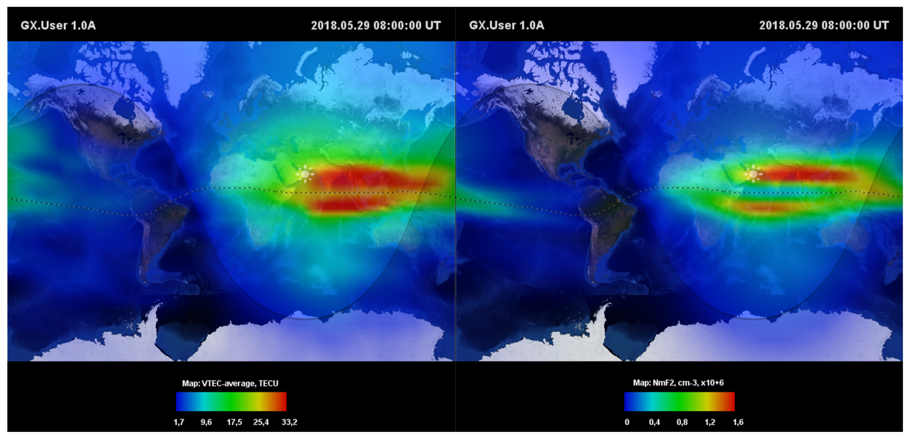
Figure 6 shows a typical result of global comparison of climate VTEC derived from 15 min GIMs maps and IRI climate NmF2 for 08:00UT on 29 May 2018, a geomagnetically quiet day on solar minimum in Mercator projection. The plots show a strong correlation between climate VTEC and NmF2, with equatorial anomaly sligtly wider and longer to the East in terms of VTEC, which is an expected behavior given the characteristics of both VTEC and NmF2 described before. Corresponding slab thickness τ is shown on
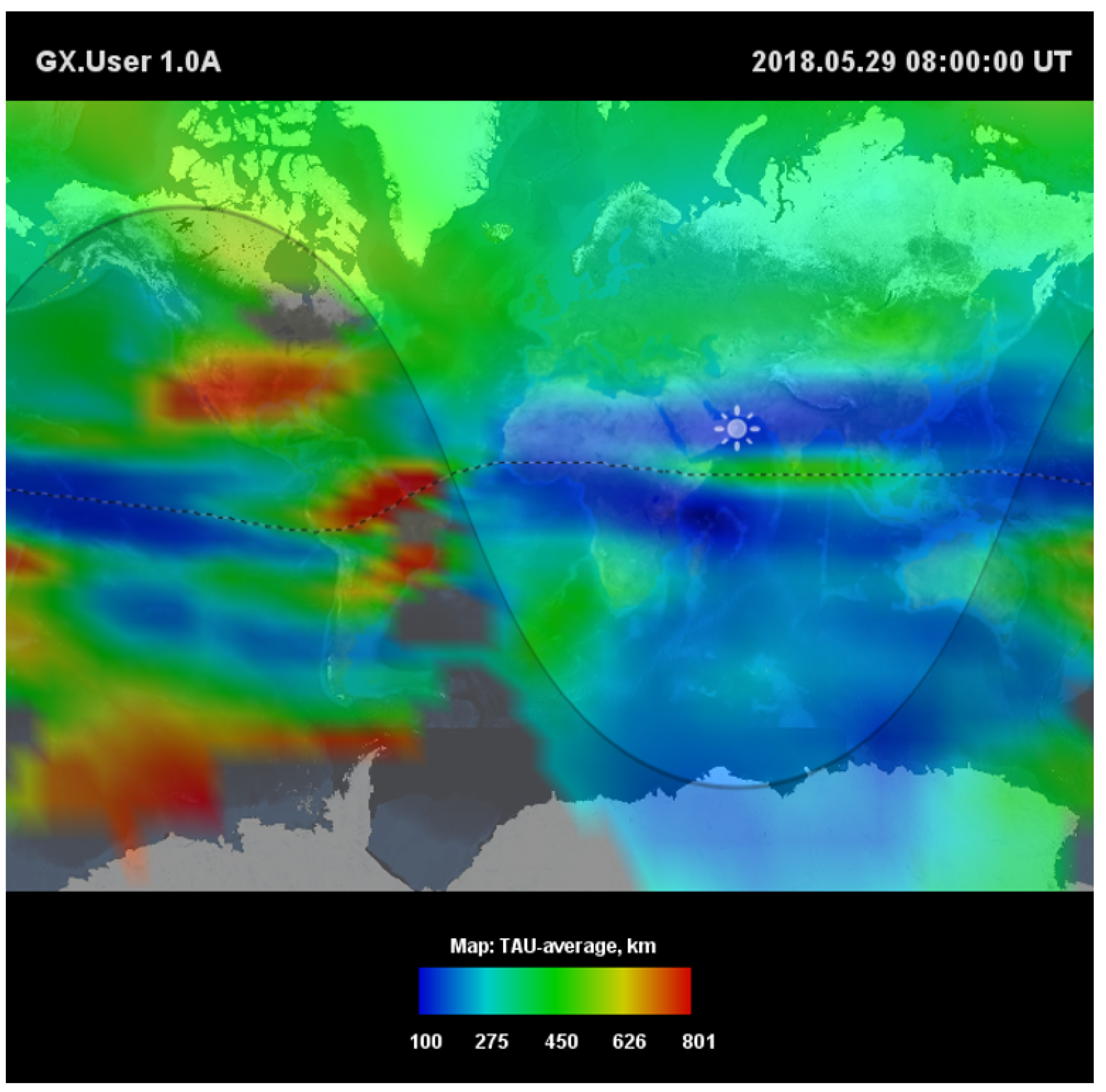
Figure 7 in Mercator projections, depicting aforementioned characteristics of slab thickness, with slab way thinner on equatorial anomaly zone and noticeably thicker just before a time of dawn, especially in mid-latitudes of the southern hemisphere.
Figure 8 shows a comparison between climate VTEC maps and NmF2 in quiet-time on the same day and time (12 UT on 30 January) of three consecutive years (2017, 2018 and 2019) in a minimum of solar cycle. Such comparison depicts a strong correlation between quiet time climate VTEC and quiet time climate NmF2. In all three cases the relation between climate VTEC (left column) and climate NmF2 (right column) depicts the characteristics shown and described on
Figure 6. The climatological properties of both VTEC and NmF2 depict the equatorial anomaly similarly, with slightly wider representation in terms of VTEC. Also it is noticeable, that NmF2 drops radically before the dawn while such behavior of VTEC is not observed.
Correlation of the quiet-time ionospheric VTEC and NmF2 is strong regardless of the local season and time of day, suggesting that on average, quiet-time VTEC is indeed driven by the contributions from the dense region of maximum ionization. Dynamics of both metrics can serve to describe timelines of the absolute electron quantity in the ionosphere. Their quotient resulting in slab thickness, as stated before, adds the capability to characterize shape of the ionospheric plasma profile, in particular the vertical extent of the ionospheric density around its peak.
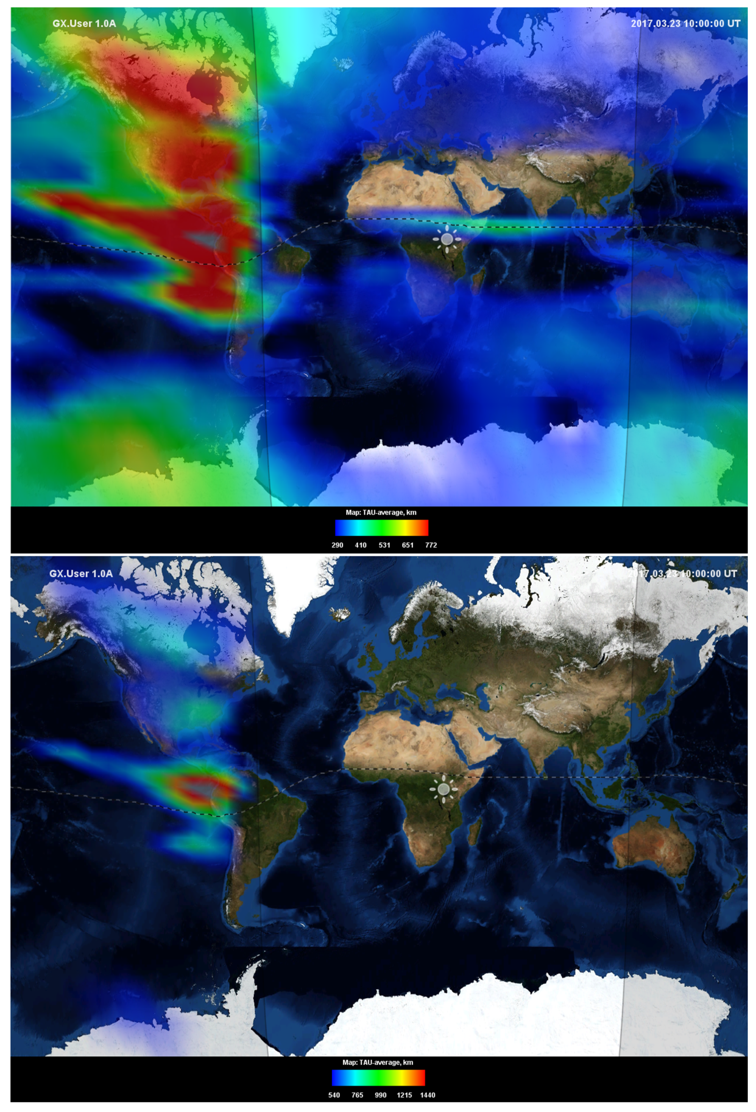
Figure 9 shows a typical climatological representation of τ with its increase just before the dawn. As mentioned before, the early morning peaks in slab thickness may appear due to the fact that sunrise is earlier at heights above the F2-layer causing some production at the topside, thus giving a tendency for TEC to lead over NmF2 that remains low, which characteristic is confirmed by our study.
4. Discussion of Path Forward
Our primary objective has been to test feasibility of fusing two independent sources of measurements for the ionospheric monitoring, GNSS-provided VTEC and GIRO-provided bottomside profile of electron density. Both resources collect their sensor information from networks of ground observatories that feature low-latency data delivery to a data processing centre. Therefore, such integrated service can support a multitude of operational systems, prone to the space weather impacts, with a prompt specification of the ionospheric conditions.
We started the integration with a task of computing a combined GNSS+GIRO data product, the slab thickness of the ionospheric/plasmaspheric plasma profile, τ. In order to validate this important capability of gleaning, even though approximately, knowledge of the vertical reshaping of plasma distribution up to the altitudes of the plasmasphere from a ground-based observatory network, our first step was to build quiet-time, averaged, "climate" maps of τ. The task required significant integration effort on both sides of the cooperation between GNSS and GIRO, starting on the level of conceptualization, through methodology, data delivery, and handling to final product dissemination and its incorporation into the GAMBIT Explorer framework for visualization and analysis. Now that a decade of climate VTEC and slab thickness maps are available, our next step will be to work on a solution to the long-standing task of incorporating climate VTEC and τ specifications in IRI.
As for the data used in the study and available through the GAMBIT Database and Explorer, the IRI is a continuous empirical model, while GIRO and IGS VTEC data are based on scattered receivers with global distribution and interpolated using techniques described in cited works. Therefore we can state that there is no lack in the data. The data quality, however, can be lower in the areas with fewer receivers, especially over the oceans. That matter has been studied and related works are cited in the paper. There is a hypothetical possibility to slightly improve the data quality in the areas with lower number of receivers, however the cost of a new station-especially GIRO ionosonde-is extremely high when compared to the improvement of data quality and does not address the issue of stations distribution over the oceans.
Choice of the Realistic Ionosphere (RION) [
4] project infrastructure for the data fusion was not a simple matter of convenience. As noted in [
6], several research groups explore scenarios of assimilating available empirical data into a "Real-Time IRI" model that transforms the underlying IRI model from its quiet-time climatology into a weather nowcast. We selected one of such Real-Time IRI solutions, IRTAM (IRI-based Real-Time Assimilative Model) for its readily available roadmap to the ionospheric weather nowcast and forecast. Our next step will be to build rapid nowcast maps of τ based on the same fusion approach proven to be successful for mapping the global climate VTEC and τ. In this approach, the 30-day average VTEC maps will be replaced by the real-time ones provided by the IGS validation centers in Europe, while NmF2 climatology by IRI will be replaced by IRTAM. As for the forecast capability, it will require additional research [
68] as the direct use of IRTAM nowcast for the short-term forecast has a validity barrier of 4 h, overcoming which would require knowledge of activity in the Sun-Earth system related to the cosmic scale processes impacting the state of the ionosphere over longer time scales. Such longer-period forecasting will necessarily involve use of additional activity indices to describe the Sun, solar wind, and magnetospheric conditions. Such effort will deviate from the classic "reference" empirical model approach based on accurate representation of measurements into the realm of physics-based arguments about overreaching system of the Heliophysics.
Our efforts so far, along with GAMBIT database infusion with historical data, have resulted in establishment of extensive testing and validating grounds in the environment of RION project that covers nearly 3 decades of corresponding historical data. With the public access to GAMBIT explorer software and VTEC/GIRO databases, we expect the RION workflow to provide scientists at large with the most up-to-date information at the lowest possible latency and consistent quality and usability. The next step will be to perform a VTEC assimilation into IRI model utilizing already prepared data sources, products, methodologies and expertise. Further cooperation goals are yet to be defined, however they will be probably focused on development of each system element in order to achieve the ambitious goal of real-time final ionospheric product availability altogether with expanded range of products, covering the whole Earth in a wide time span and great spatial and temporal resolution.
An intriguing possibility for such enhancement is given by novel real-time and short period forecast VTEC global products described by [
69,
70]. As IGS IONO WG members and contributors develop and enhance their real-time ionospheric products and a combined real-time GIM product [
24] is being prepared, it may lead in the future to the assimilation of those products or their derivatives into the Real-Time IRI, further enhancing its capabilities of the ionospheric weather nowcast.
5. Conclusions
Advanced digital technologies for signal processing have brought a quiet revolution to radio-frequency (RF) remote plasma imaging. Renewed interest in RF remote sensing is supported by the growing demand of high accuracy specification of the signal propagation effects for modern applications such as precision navigation and HF geolocation. New instrumentation is more capable and cost-effective, allowing sensor networks to grow internationally. Matching to this fundamental technology advancements, the assimilative modeling community pursues new generation models that accept heterogeneous data sources from providers in vastly different domains of RF.
Our effort to introduce global climate TEC maps is an important first step in data fusion for different worlds of the ionospheric plasma sensing: GNSS and GIRO. The outcome of this effort is a tight cooperation between three working groups of URSI and COSPAR: IGS Ionosphere, International Reference Ionosphere, and Ionosonde Network Advisory Group. Three science teams have combined their efforts to make this cooperation possible: Universitat Politècnica de Catalunya in Spain provided UQRG maps of VTEC, University of Massachusetts Lowell in the USA provided GAMBIT database and explorer software, and University of Warmia and Mazury in Poland linked this capabilities to implement Climate VTEC and climate slab thickness mapping.
The ultimate goal of this effort is to depict the actual ionospheric state in real time. As pointed out earlier, assessing plasma conditions using the nowcast snapshot of its current state is inefficient, if possible at all, without inclusion of climatology-based prediction as the reference. Provision of the climate reference got simply overlooked by the working group member entities and other researchers that were focusing their efforts on provision of the weather nowcast at given instant and location. Because of inherent latency in the data management and associated processing, such service has been limited to only retrospective depictions (backcasts) and could not approach the real-time until only recently.
Although slab thickness computation may appear simple, the fact that its outcomes are sensible from the point of underlying physics of the ionosphere is significant on its own. The measurements of VTEC and NmF2 that go into the computation are from different domains of remote sensing, both tainted with the accuracy and bias of the estimations. Remarkably, the efforts at two communities of GNSS and GIRO that went into generation of the input datasets and their conditioning for subsequent analyses were proven successful.
We believe that a step towards the objective of real-time nowcast has been made with the climate VTEC and slab thickness maps developed in cooperation of GNSS and GIRO. There is still much work remaining to do as new opportunities for cooperation and new data fusion products appear. Further detail of the fusion approaches and their synergies and correlations will be needed to meet the challenge.
Author Contributions
Conceptualization: A.K., I.G., A.F.; Methodology: I.G., A.K., D.B., B.R.; Software: A.F., K.K. and P.F.; Validation: A.F., A.K., I.G. and D.B.; Formal analysis: A.F., I.G., A.K. and D.B.; Investigation, resources and data curation: M.H.-P., A.F., K.K., Z.L., N.W., P.F., I.Z., I.C., D.R.D. and A.G.-R.; Writing—original draft preparation: A.F., I.G., A.K. and D.B.; Writing—review and editing: A.F., I.G., A.K. and D.B.; Visualization: A.F. and I.G.; Supervision: A.K., I.G., D.B. and B.R.; Project administration: A.K.; Funding acquisition: A.K. All authors have read and agreed to the published version of the manuscript.
Funding
The UWM contribution is supported by the National Centre for Research and Development, Poland, through grant ARTEMIS (decision numbers DWM/PL-CHN/97/2019 and WPC1/ARTEMIS/2019) and the National Science Centre, Poland, through grant 2017/27/B/ST10/02190. The UWM authors thank also for their support the Ministry of Science and Higher Education (MSHE), Poland, for granting funds for the Polish contribution to the International LOFAR Telescope (MSHE decision number DIR/WK/2016/2017/05-1) and for maintenance of the LOFAR PL-612 Baldy (MSHE decision number 59/E-383/SPUB/SP/2019.1).
Acknowledgments
The authors thank International GNSS Service for sharing the data used in this paper as well as IGS Ionosphere Working Group and COSPAR/URSI International Reference Ionosphere Working Group for initiating this approach and method and for data and products for comparison and validation. All average-VTEC, NmF2, and slab thickness datasets are released to open public domain, available via GAMBIT Explorer (download at
http://giro.uml.edu/GAMBIT) for display and export in plain text and IONEX formats.
Conflicts of Interest
The authors declare no conflict of interest.
Abbreviations
The following abbreviations are used in this manuscript:
| IGS | International GNSS Service |
| IGS IONO WG | IGS’ Ionosphere Working Group |
| TEC | Total Electron Content |
| VTEC | Vertical Total Electron Content |
| ROTI | Rate of TEC Index |
| IRI | International Reference Ionosphere |
| GIRO | Global Ionospheric Radio Observatory |
| GAMBIT | Global Assimilative Model of Bottomside Ionosphere Timeline |
| IRTAM | RI-based Real-time Assimilative Model |
| LGDC | Lowell GIRO Data Center |
| COSPAR | Committee on Space Research |
| ICVC | IGS Ionosphere Combination and Validation Center |
| UWM | University of Warmia and Mazury in Olsztyn, Poland |
| IAAC | Ionospheric Associate Analysis Center |
| CODE | Center for Orbit Determination in Europe |
| ESA | European Space Agency |
| JPL | NASA Jet Propulsion Laboratory |
| UPC | Technical University of Catalonia |
| NRCAN | National Resources Canada |
| CAS | Chinese Academy of Sciences |
| WHU | Wuhan University |
| DGFI-TUM | Technical University of Munich |
| CNES | Centre National d’Études Spatiales |
| URSI | International Union of Radio Science |
| ISO | International Standardization Organization |
| UQRG | UPC’s rapid GIM |
References
- Hernández-Pajares, M.; Juan, J.M.; Sanz, J.; Orus, R.; Garcia-Rigo, A.; Feltens, J.; Komjathy, A.; Schaer, S.C.; Krankowski, A. The IGS VTEC maps: A reliable source of ionospheric information since 1998. J. Geod. 2009, 83, 263–275. [Google Scholar] [CrossRef]
- García-Rigo, A.; Monte, E.; Hernández-Pajares, M.; Juan, J.M.; Sanz, J.; Aragón-Angel, A.; Salazar, D. Global prediction of the vertical total electron content of the ionosphere based on GPS data. Radio Sci. 2011, 46, RS0D25. [Google Scholar] [CrossRef]
- Gulyaeva, T.L.; Arikan, F.; Hernández-Pajares, M.; Stanislawska, I. 2013, GIM-TEC adaptive ionospheric weather assessment and forecast system. J. Atmos. Sol.-Terr. Phys. 2013, 102, 329–340. [Google Scholar] [CrossRef]
- Galkin, I.A.; Reinisch, B.W.; Bilitza, D. Realistic Ionosphere: Real-time ionosonde service for ISWI. SunGe 2018, 13, 173–178. [Google Scholar] [CrossRef]
- Reinisch, B.W.; Galkin, I.A. Global Ionospheric Radio Observatory (GIRO). Earth Planets Space 2011, 63, 377–381. [Google Scholar] [CrossRef]
- Bilitza, D.; Altadill, D.; Truhlik, V.; Shubin, V.; Galkin, I.; Reinisch, B.; Huang, X. International Reference Ionosphere 2016: From ionospheric climate to real-time weather predictions. Space Weather 2017, 15, 418–429. [Google Scholar] [CrossRef]
- Bilitza, D. IRI the International Standard for the Ionosphere. Adv. Radio Sci. 2018, 16, 1–11. [Google Scholar] [CrossRef]
- Shim, J.S.; Kuznetsova, M.; Rastätter, L.; Hesse, M.; Bilitza, D.; Codrescu, M.; Emery, B.; Foster, B.; FullerRowell, T.; Huba, J.; et al. CEDAR Electrodynamics Thermosphere Ionosphere 1 (ETI) Challenge for Systematic Assessment of Ionosphere/ Thermosphere Models 1: NmF2, hmF2, and Vertical Drift Using Ground Based Observations. Space Weather 2011, 9, S12003. [Google Scholar] [CrossRef]
- Shim, J.S.; Kuznetsova, M.; Rastätter, L.; Bilitza, D.; Butala, M.; Codrescu, M.; Emery, B.A.; Foster, B.; Fuller-rowell, T.J.; Huba, J.; et al. CEDAR Electrodynamics Thermosphere Ionosphere (ETI) Challenge for systematic assessment of ionosphere/thermosphere models: Electron density, neutral density, NmF2, and hmF2 using space based observations. Space Weather 2012, 10, 1–16. [Google Scholar] [CrossRef]
- Shim, J.S.; Kuznetsova, M.; Rastätter, L.; Bilitza, D.; Butala, M.; Codrescu, M.; Emery, B.A.; Foster, B.; Fuller-Rowell, T.J.; Huba, J.; et al. Systematic Evaluation of Ionosphere/Thermosphere (IT) Models. In Modeling the Ionosphere-Thermosphere System; Huba, J., Schunk, R., Khazanov, G., Eds.; John Wiley & Sons, Ltd.: Chichester, UK, 2014. [Google Scholar] [CrossRef]
- Shim, J.S.; Rastätter, L.; Kuznetsova, M.; Bilitza, D.; Codrescu, M.; Coster, A.J.; Emery, B.A.; Fedrizzi, M.; Förster, M.; Fuller-Rowell, T.J.; et al. CEDAR-GEM challenge for systematic assessment of Ionosphere/thermosphere models in predicting TEC during the 2006 December storm event. Space Weather 2017, 15, 1238–1256. [Google Scholar] [CrossRef]
- Shim, J.S.; Tsagouri, I.; Goncharenko, L.; Rastaetter, L.; Kuznetsova, M.; Bilitza, D.; Codrescu, M.V.; Coster, A.J.; Solomon, S.C.; Fedrizzi, M.; et al. Validation of ionospheric specifications during geomagnetic storms: TEC and foF2 during the 2013 March storm event. Space Weather 2018, 16, 1686–1701. [Google Scholar] [CrossRef]
- Fuller-Rowell, T. Real-Time IRI Task Force, IRI Workshop, May 4, 2009, Colorado Springs, CO. 2009. Available online: http://irimodel.org/docs/IRI-RT_Summary.pdf (accessed on 4 September 2020).
- Galkin; Reinisch,, I.A.; Huang,, B.W.; Bilitza, X. DAssimilation of GIRO data into a real-time IRI. Radio Sci. 2012, 47, RS0L07. [Google Scholar] [CrossRef]
- Galkin, I.A.; Reinisch, B.W.; Vesnin, A.M.; Bilitza, D.; Fridman, S.; Habarulema, J.B.; Veliz, O. Assimilation of Sparse Continuous Near-Earth Weather Measurements by NECTAR Model Morphing. Space Weather 2020, e2020SW002463. [Google Scholar] [CrossRef]
- Galkin, I.; Vesnin, A.; Kozlov, A.; Huang, X.; Reinisch, B. GAMBIT Database and Explorer. In Proceedings of the 2015 1st URSI Atlantic Radio Science Conference (URSI AT-RASC), Gran Canaria, Spain, 16–24 May 2015. [Google Scholar] [CrossRef]
- Villiger, A.; Dach, R. (Eds.) International GNSS Service Technical Report 2019 (IGS Annual Report); IGS Central Bureau and University of Bern; Bern Open Publishing: Bern, Switzerland, 2020. [Google Scholar] [CrossRef]
- Titheridge, J.E. The slab thickness of the mid-latitude ionosphere. Planet. Space Sci. 1973, 21, 1775–1793. [Google Scholar] [CrossRef]
- Hernández-Pajares, M.; Juan, J.M.; Sanz, J. High resolution TEC monitoring method using permanent ground GPS receivers. Geophys. Res. Lett. 1997, 24, 1643–1646. [Google Scholar] [CrossRef]
- Feltens, J. The International GPS Service (IGS) Ionosphere Working Group. Adv. Space Res. 2003, 31, 635–644. [Google Scholar] [CrossRef]
- Hernández-Pajares, M. IGS Ionosphere WG Status Report: Performance of IGS Ionosphere TEC Maps-Position Paper; IGS: Barcelona, Spain, 2004. [Google Scholar]
- Feltens, J.; Schaer, S. IGS Products for the Ionosphere, IGS Position Paper. In Proceedings of the IGS Analysis Centers Workshop, Darmstadt, Germany, 9 February 1998; pp. 225–232. [Google Scholar]
- Cherniak, I.; Krankowski, A.; Zakharenkova, I. ROTI Maps: A new IGS ionospheric product characterizing the ionospheric irregularities occurrence. GPS Solut. 2018, 22, 69. [Google Scholar] [CrossRef]
- Li, Z.; Wang, N.; Hernández-Pajares, M. IGS real-time service for global ionospheric total electron content modeling. J. Geod. 2020, 94, 32. [Google Scholar] [CrossRef]
- Roma-Dollase, D.; Hernández-Pajares, M.; Krankowski, A.; Kotulak, K.; Ghoddousi-Fard, R.; Yuan, Y.; Li, Z.; Zhang, H.; Shi, C.; Wang, C.; et al. Consistency of seven different GNSS global ionospheric mapping techniques during one solar cycle. J. Geod. 2018, 92, 691. [Google Scholar] [CrossRef]
- Krankowski, A.; Hernandez-Pajares, M. Ionosphere Working Group Technical Report 2018. In International GNSS Service Technical Report 2018 (IGS Annual Report); Villiger, A., Dach, R., Eds.; IGS Central Bureau and University of Bern; Bern Open Publishing: Bern, Switzerland, 2019; pp. 185–190. [Google Scholar] [CrossRef]
- Schaer, S. Mapping and Predicting the Earth’S Ionosphere Using the Global Positioning System, French Studies of the Eighteenth and Nineteenth Centuries; Institut für Geodäsie und Photogrammetrie, Eidg. Technische Hochschule Zürich: Zürich, Switzerland, 1999. [Google Scholar]
- Okoh, D. GPS Modeling of the Ionosphere Using Computer Neural Networks. In Hashimov, Multifunctional Operation and Application of GPS, BoD–Books on Demand; Rustam, B., Rustamov, A.M., Eds.; Intechopen: London, UK, 2018. [Google Scholar] [CrossRef]
- Kotulak, K.; Froń, A.; Krankowski, A.; Pulido, G.O.; Hernández-Pajares, M. Sibsonian and non-Sibsonian natural neighbour interpolation of the total electron content value. Acta Geophys. 2017, 65, 13. [Google Scholar] [CrossRef]
- Orus, R.; Hernández-Pajares, M.; Juan, J.M.; Sanz, J. Improvement of global ionospheric VTEC maps by using kriging interpolation technique. J. Atmos. -Sol. Phys. 2005, 67, 1598–1609. [Google Scholar]
- Hernández-Pajares, M.; Juan, J.M.; Sanz, J. New approaches in global ionospheric determination using ground GPS data. J. Atmos.Sol.-Terrest. Phys. 1999, 61, 1237–1247. [Google Scholar] [CrossRef]
- Garcia-Rigo, A.; Hernandez, M.; Orús, R. UPC contributions to GNSS monitoring of ionosphere in the frame of the IGS Iono-WG. A: International GNSS Service Workshop. In Proceedings of the IGS Workshop 2014 Celebrating 20 Years of Service: 1994–2014, Pasadena, CA, USA, 23–27 June 2014; p. 1. [Google Scholar]
- Hernández-Pajares, M.; Roma-Dollase, D.; Krankowski, A.; García-Rigo, A.; Orús-Pérez, R. Methodology and consistency of slant and vertical assessments for ionospheric electron content models. J. Geod. 2017, 91, 1405–1414. [Google Scholar]
- Azpilicueta, F.; Brunini, C. Analysis of the bias between TOPEX and GPS vTEC determinations. J. Geod. 2009, 83, 121–127. [Google Scholar]
- Hernández-Pajares, M.; Roma-Dollase, D.; García-Rigo, A.; Krankowski, A. Assessment of VTEC provided by DGFI and IGS GNSS-GIMs vs JASON3. In Proceedings of the IGS Workshop 2018, Wuhan, China, 29 October–2 November 2018. [Google Scholar]
- Bilitza, D. The International Reference Ionosphere-Status 2013. Adv. Space Res. 2015, 55, 1914–1927. [Google Scholar]
- Bilitza, D.; Hernández-Pajares, M.; Juan, J.M.; Sanz, J. Comparison between IRI and GPS-IGS Derived Electron Content during 1991–1997. Phys. Chem. Earth C 1999, 24, 311–319. [Google Scholar]
- Zakharenkova, I.E.; Cherniak, I.V.; Krankowski, A.; Shagimuratov, I.I. Vertical TEC representation by IRI 2012 and IRI Plas models for European midlatitudes. Adv. Space Res. 2015, 55, 2070–2076. [Google Scholar]
- Wang, S.; Huang, S.; Fang, H.; Wang, Y. Evaluation and correction of the IRI2016 topside ionospheric electron density model. Adv. Space Res. 2016, 58, 1229–1241. [Google Scholar]
- Bilitza, D.; Bhardwaj, S.; Koblinsky, C. Improved IRI predictions for the GEOSAT time period. Adv. Space. Res. 1997, 20, 1755–1760. [Google Scholar] [CrossRef]
- Komjathy, A.; Langley, R.; Bilitza, D. Ingesting GPS-derived TEC data into the international reference ionosphere for single frequency radar altimeter ionospheric delay corrections. Adv. Space Res. 1998, 22, 793–802. [Google Scholar]
- Hernáez-Pajares, M.; Juan, J.; Sanz, J.; Bilitza, D. Combining GPS measurements and IRI model values for space weather specification. Adv. Space Res. 2002, 29, 949–958. [Google Scholar] [CrossRef]
- Pignalberi, A.; Pezzopane, M.; Rizzi, R. Modeling the lower part of the topside ionospheric vertical electron density profile over the European region by means of Swarm satellites data and IRI UP method. Space Weather 2018, 16, 304–320. [Google Scholar] [CrossRef]
- Pignalberi, A.; Pietrella, M.; Pezzopane, M.; Rizzi, R. Improvements and validation of the IRI UP method under moderate, strong, and severe geomagnetic storms. Earth Planets Space 2018, 70, 180. [Google Scholar] [CrossRef]
- Pignalberi, A.; Habarulema, J.B.; Pezzopane, M.; Rizzi, R. On the development of a method for updating an empirical climatological ionospheric model by means of assimilated vTEC measurements from a GNSS receiver network. Space Weather 2019, 17, 1131–1164. [Google Scholar] [CrossRef]
- Garcia-Fernández, M.; Hernández-Pajares, M.; Juan, J.M.; Sanz, J.; Orus, R.; Coisson, P.; Nava, B.; Radicella, S.M. Combining ionosonde with ground GPS data for electron density estimation. J. Atmos. Sol.-Terr. Phys. 2003, 65, 683–691. [Google Scholar] [CrossRef]
- Huang, X.; Reinisch, B.W. Real time HF raytracing through a tilted ionosphere. Radio Sci. 2006, 41, RS5S47. [Google Scholar] [CrossRef]
- Reinisch, B.W.; Galkin, I.A.; Khmyrov, G.M.; Kozlov, A.V.; Bibl, K.; Lisysyan, I.A.; Cheney, G.P.; Huang, X.; Kitrosser, D.F.; Paznukhov, V.V.; et al. New Digisonde for research and monitoring applications. Radio Sci. 2009, 44, RS0A24. [Google Scholar] [CrossRef]
- Gerzen, T.; Jakowski, N.; Wilken, V.; Hoque, M. Reconstruction of F2 layer peak electron density based on operational vertical Total Electron Content maps. Ann. Geophysicae. 2013, 31, 1241–1249. [Google Scholar] [CrossRef][Green Version]
- Piggott, W.R.; Rawer, K. World Data Center a for Solar-Terrestrial Physics U.R.S.I Handbook of Ionogram Interpretation and Reduction (Boulder, Colorado, World Data Center a for Solar-Terrestrial Physics; NOAA: Boulder, CO, USA, 1972. [Google Scholar]
- Yun, J.; Kim, Y.; Kim, E.; Kwak, Y.-S.; Hong, S. Unusual Enhancements of NmF2 in Anyang Ionosonde Data. J. Astron. Space Sci. 2013, 30, 223–230. [Google Scholar] [CrossRef][Green Version]
- Reinisch, B.; Galkin, I.; Belehaki, A.; Paznukhov, V.; Huang, X.; Altadill, D.; Buresova, D.; Mielich, J.; Verhulst, T.; Stankov, S.; et al. Pilot Ionosonde Network for Identification of Traveling Ionospheric Disturbances. Radio Sci. 2018, 53, 365–378. [Google Scholar] [CrossRef]
- Altadill, D.; Segarra, A.; Blanch, E.; Juan, J.; Paznukhov, V.; Buresova, D.; Galkin, I.; Reinisch, B.; Belehaki, A. A method for real-time identification and tracking of traveling ionospheric disturbances using ionosonde data: First results. J. Space Weather Space Clim. 2020, 10, 2. [Google Scholar] [CrossRef]
- Jayachran, B.; Krishnankutty, T.; Gulyaeva, T. Climatology of ionospheric slab thickness. Ann. Geophys. 2004, 22. [Google Scholar] [CrossRef]
- Jakowski, N.; Stankov, S.M.; Wilken, V.; Borries, C.; Altadill, D.; Chum, J.; Buresova, D.; Boska, J.; Sauli, P.; Hruska, F.; et al. Ionospheric behavior over Europe during the solar eclipse of 3 October 2005. J. Atmos. Sol.-Terr. Phys. 2008, 70, 836–853. [Google Scholar] [CrossRef]
- Huang, Z.; Yuan, H. Climatology of the ionospheric slab thickness along the longitude of 120 degrees E in China and its adjacent region during the solar minimum years of 2007–2009. Ann. Geophys. 2015, 33, 1311–1319. [Google Scholar] [CrossRef]
- Huang, H.; Liu, L.; Chen, Y.; Le, H.; Wan, W. A global picture of ionospheric slab thickness derived from GIM TEC and COSMIC radio occultation observations. J. Geophys. Res. Space Phys. 2016, 121, 867–880. [Google Scholar] [CrossRef]
- Iwamoto, I.; Katoh, H.; Maruyama, T.; Minakoshi, H.; Watari, S.; Igarashi, K. Latitudinal variation of solar flux dependence in the topside plasma density: Comparison between IRI model and observations. Adv. Space Res. 2002, 29, 877–882. [Google Scholar] [CrossRef]
- Kenpankho, P.; Supnithi, P.; Tsugawa, T. Variation of ionospheric slab thickness observations at Chumphon equatorial magnetic location. Earth Planet Space 2011, 63, 359–364. [Google Scholar] [CrossRef][Green Version]
- Stankov, S.M.; Warnant, R. Ionospheric slab thickness–Analysis, modelling and monitoring. Adv. Space Res. 2009, 44, 1295–1303. [Google Scholar] [CrossRef]
- Kouris, S.S.; Polimeris, K.V.; Ciraolo, L.; Fotiadis, D.N. Seasonal dependence of TEC and SLAB thickness. Adv. Space Res. 2009, 44, 715–724. [Google Scholar] [CrossRef]
- Chuo, Y.J.; Lee, C.C.; Chen, W.S. Comparison of ionospheric equivalent slab thickness with bottomside digisonde profile over Wuhan. J. Atmos. Sol.-Terr. Phys. 2010, 72, 528–533. [Google Scholar] [CrossRef]
- Jakowski, N.; Hoque, M.M.; Mielich, J.; Hall, C. Equivalent slab thickness of the ionosphere over Europe as an indicator of long-term temperature changes in the thermosphere. J. Atmos. -Sol. Phys. 2017, 163, 91–102. [Google Scholar]
- Gallagher, D.L.; Craven, P.D.; Comfort, R.H. Global Core Plasma Model. J. Geophys. Res. 2000, 105, 18819–18833. [Google Scholar]
- Ozhogin, P.; Tu, J.; Song, P.; Reinisch, B.W. Field-aligned distribution of the plasmaspheric electron density: An empirical model derived from the IMAGE RPI measurements. J. Geophys. Res. 2012, 117. [Google Scholar] [CrossRef]
- Chasovitin, Y.K.; Gulyaeva, T.L.; Deminov, M.G.; Ivanova, S.E. Russian Standard Model of the Ionosphere (SMI), COST 251 Tech. Doc. TD(98)005; Rutherford Appleton Lab.: Oxford, UK, 1998; pp. 161–172. [Google Scholar]
- Gulyaeva, T.L.; Titheridge, J.E. Advanced specification of electron density and temperature in the IRI ionosphere-plasmasphere model. Adv. Space Res. 2006, 38, 2587–2595. [Google Scholar]
- Galkin, I.; Song, P.; Reinisch, B.; Bilitza, D. From Ionospheric Weather Nowcast to Forecast: 1. Choice of IRTAM Basis. In Proceedings of the 2018 2nd URSI Atlantic Radio Science Meeting (AT-RASC), Meloneras, Spain, 28 May–1 June 2018. [Google Scholar]
- Wang, C.; Xin, S.; Liu, X. Prediction of global ionospheric VTEC maps using an adaptive autoregressive model. Earth Planets Space 2018, 70, 18. [Google Scholar] [CrossRef]
- Ren, X.; Chen, J.; Li, X. Performance evaluation of real-time global ionospheric maps provided by different IGS analysis centers. GPS Solut. 2019, 113, 113. [Google Scholar] [CrossRef]
| Publisher’s Note: MDPI stays neutral with regard to jurisdictional claims in published maps and institutional affiliations. |
© 2020 by the authors. Licensee MDPI, Basel, Switzerland. This article is an open access article distributed under the terms and conditions of the Creative Commons Attribution (CC BY) license (http://creativecommons.org/licenses/by/4.0/).

 ,
, 


