Effect of Wind Transport of Turbulent Inhomogeneities on Estimation of the Turbulence Energy Dissipation Rate from Measurements by a Conically Scanning Coherent Doppler Lidar

Abstract

A method for estimation of the turbulent energy dissipation rate from measurements by a conically scanning pulsed coherent Doppler lidar (PCDL), with allowance for the wind transport of turbulent velocity fluctuations, has been developed. The method has been tested in comparative atmospheric experiments with a Stream Line PCDL (Halo Photonics, Brockamin, Worcester, United Kingdom) and a sonic anemometer. It has been demonstrated that the method provides unbiased estimates of the dissipation rate at arbitrarily large ratios of the mean wind velocity to the linear scanning speed.

1. Introduction

In the atmospheric boundary layer (ABL), the wind air flow is always turbulent and can be represented as a set of random vortices of various scales, with cascade energy transfer from the largest vortices to small vortices, up to the dissipation of energy into heat. In the inertial subrange of the scales of these eddies, the local spatial structure of the wind flow depends only on the dissipation rate of the kinetic energy of turbulence. Information on the dissipation rate is important for studying the spatial structure of turbulence and the dynamics of ABL and for constructing a mathematical model of ABL designed to solve a wide range of practical problems (weather forecasting, air transport safety, diffusion of atmospheric impurities, etc.).

The advent of pulsed coherent Doppler lidars (PCDLs), providing high spatial and temporal resolution of wind velocity measurements—in particular, all-fiber PCDLs such as Stream Line (Halo Photonics, Brockamin, Worcester, United Kingdom) [1] and WindCube 200s (Leosphere, France) [2]—has led to great potential for the investigation of wind turbulence in the atmospheric boundary layer [3,4,5,6,7,8,9,10,11,12,13,14]. In Smalikho and Banakh’s work [14], a method was proposed for the determination of such turbulence parameters as the turbulence kinetic energy, turbulence energy dissipation rate, integral scale of turbulence and momentum fluxes from lidar measurements with conical scanning (see Figure 1 or the paper [15]). In the case of conical scanning, a probing beam revolves around the vertical axis at an angle $\phi$ to the horizontal, with a constant angular rate ω_s, and for every measurement height $h$, the probing volume moves along the circle of the radius $R^{\prime }=h/\tan \phi$ with a certain linear speed. It is shown in the authors’ work [14] that estimates of the turbulence energy dissipation rate obtained from Stream Line lidar data using this method are in a good agreement with the dissipation rate estimates from the data of sonic anemometers.

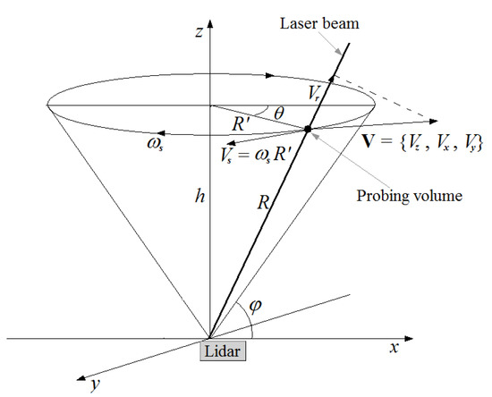
Figure 1. Geometry of measurement by a pulsed coherent Doppler lidar with conical scanning by laser beam.

An important feature of determination of the wind vector and wind turbulence parameters from lidar data is the need to consider the spatial averaging of the measured radial velocity over the probing volume. Just the consideration of spatial averaging provides for a correct estimation of the dissipation rate from lidar data [14]. Even though the probing volume of the Stream Line lidar is small, its longitudinal dimension is $\Delta z$ = 30 m [16].

The method proposed in the authors’ work [14] assumes that the mean wind velocity is much smaller than the linear speed of motion of the probing volume along the circle of the scanning cone base at the probing height $h$. However, at small measurement heights and in strong wind, this condition is not always fulfilled. In this paper, the method from the authors’ work [14] is generalized to the case of an arbitrary ratio between the mean wind velocity and the linear scanning speed at the probing height. The method was tested in atmospheric experiments, and the results of these tests are presented.

2. Basic Equations for Estimation of the Turbulence Energy Dissipation Rate from Measurements by PCDL with Conical Scanning

In the case of conical scanning, after primary processing of PCDL echo signals, we obtain an array of estimates of the radial velocity V_L(θ_m;n) for different distances $R$ from the lidar and azimuth angles ${\theta }_m=m\Delta \theta$, where $m=0,1,2,\dots ,M-1$, Δθ is the azimuth angle resolution, $(M-1)\Delta \theta$ = 360°, and $n=1,2,3,4,\dots$ is the scan number. On the assumption that the wind is a stationary process (within one hour) and horizontally statistically homogeneous (within the circle of the scanning cone base), the mean wind vector $<V(h)>=\{<V_z>,<V_x>,<V_y>\}$ is estimated from the array $V_L({\theta }_m;n)$ for the height $h=R\sin \phi$ by sine-wave least-square fitting [17]. Here, $V_z$ is the vertical component of the wind velocity vector $V=\{V_z,V_x,V_y\}$, $V_x$, $V_y$ are its horizontal components, and the angular brackets are for the ensemble averaging. Then, the array of random components of the lidar estimates of radial velocities is calculated for the same height h as

$$V_L^{\prime }({\theta }_m;n)=V_L({\theta }_m;n)-S({\theta }_m)\cdot <V(h){>}_N,$$

(1)

where $S(\theta )=\{\sin \phi ,\cos \phi \cos \theta ,\cos \phi \sin \theta \}$ is the unit vector along the optical axis of the probing beam and $<f(n){>}_N=\frac{1}{N}{\displaystyle \sum _{n^{\prime }=n-N/2}^{n+N/2-1}f(n+n^{\prime })}$ is the average over N scans. This array is used to calculate the azimuth structure function ${\overline{D}}_L(l\Delta \theta )$ of radial velocity fluctuations (the function averaged over all azimuth angles ${\theta }_m$) by the following equation:

$${\overline{D}}_L(l\Delta \theta )=<\frac{1}{M-l}{\displaystyle \sum _{m=0}^{M-l-1}{[V_L^{\prime }({\theta }_m+l\Delta \theta ;n)-V_L^{\prime }({\theta }_m;n)]}^2}{>}_N,$$

(2)

where $l=1,2,3,4,\dots ,L<<M$.

During scanning, the center of the probing volume moves at a level $h=R\sin \phi$ along the circle of the radius $R^{\prime }=R\cos \phi$ and passes the distance $L_c=2\pi R^{\prime }$ for one scan. The linear speed of the probing volume along this circle is $V_s=L_c/T_{\mathrm{scan}}={\omega }_s{R}^{\prime }$, where ${\omega }_s=2\pi /T_{\mathrm{scan}}$ is the angular scanning rate, and $T_{\mathrm{scan}}$ is the duration of one scan. According to Figure 1, the linear scanning speed $V_s$ depends on the height $h$, elevation angle $\phi$, and time $T_{\mathrm{scan}}$ as

$$V_s(h,\phi ,T_{\mathrm{scan}})=\frac{2\pi h}{T_{\mathrm{scan}}\tan \phi }.$$

(3)

We introduced the parameter $\mu =U/V_s$, where $U=|<U>|$ is the mean wind speed, $U=\{V_x,V_y\}$. It was shown in the authors’ work [14] that, under the condition $\mu <<1$, when the transport of turbulent inhomogeneities by the mean wind can be neglected in comparison with the linear scanning speed, the azimuth structure function (ensemble average) of radial velocity measured by a conically scanning PCDL can be represented in the form

$$<{\overline{D}}_L(l\Delta \theta )>=D_{\perp }(l\Delta y)+2{\sigma }_e^2.$$

(4)

In Equation (4), $\Delta y=\Delta \theta R^{\prime }=\Delta \theta h/\tan \phi$ is the transverse dimension of the probing volume (separation between the centers of neighboring probing volumes on the circle of the scanning cone base at the height $h$), $D_{\perp }(l\Delta y)={\epsilon }^{2/3}{A}_{\perp }(l\Delta y)$ is the transverse spatial structure function of the radial velocity averaged over the probing volume, $\epsilon$ is the turbulence energy dissipation rate, and ${\sigma }_e$ is the instrumental error of the radial velocity estimate. Equation (4) is valid for distances within the inertial subrange $l\Delta y<L_V$, where $L_V$ is the integral scale of turbulence, and under the condition $l\Delta \theta \le \pi /20$ = 9°.

According to Equation (20) in [14], the function $A_{\perp }(l\Delta y)\equiv A(l\Delta y)$ can be represented in the form

$$A_{\perp }(l\Delta y)=2{\displaystyle \underset{0}{\overset{\infty }{\int }}d{\kappa }_1}{\displaystyle \underset{0}{\overset{\infty }{\int }}d{\kappa }_2}\Phi ({\kappa }_1,{\kappa }_2)H_{\parallel }({\kappa }_1)H_{\perp }({\kappa }_2)[1-\cos (2\pi l\Delta y{\kappa }_2)],$$

(5)

where

$$\Phi ({\kappa }_1,{\kappa }_2)=0.0652{\left({\kappa }_1^2+{\kappa }_2^2\right)}^{-4/3}\left[1+(8/3){\kappa }_2^2/\left({\kappa }_1^2+{\kappa }_2^2\right)\right],$$

(6)

$$H_{\parallel }({\kappa }_1)={\left[\exp \{-{(\pi \Delta p{\kappa }_1)}^2\}\sin \mathrm{c}(\pi \Delta R{\kappa }_1)\right]}^2$$

(7)

is the longitudinal transfer function of the low-pass filter,

$$H_{\perp }({\kappa }_2)={\left[\sin \mathrm{c}(\pi \Delta y{\kappa }_2)\right]}^2$$

(8)

is the transverse transfer function of the low-pass filter, $\Delta p=c{\sigma }_p/2$, $\Delta R=c{T}_W/2$, $c$ is the speed of light, ${\sigma }_p={\tau }_p/\left(2\sqrt{\ln 2}\right)$, ${\tau }_p$ is the probing pulse duration, $T_W$ is the time window width, and $\sin c(x)=\sin (x)/x$ [18]. In our measurements by the Stream Line lidar, $\Delta p$ = 15.3 m and $\Delta R$ = 18 m.

Equation (21) in the authors’ work [14] is used to estimate the turbulence energy dissipation rate under the condition μ = 0 ($\mu <<1$). Let the method for estimation of the dissipation rate by Equation (21) in [14] be called Method 1 and the estimate of the dissipation rate by Method 1 be designated as ${\epsilon }_1$. The method for estimation of the dissipation rate with regard to the transport of turbulent inhomogeneities by the mean wind at $\mu \ne 0$ is referred to as Method 2 and the corresponding estimate of the dissipation rate by Method 2 is designated as ${\epsilon }_2$.

By analogy with [14], we represent the estimate of the dissipation rate in the form

$${\epsilon }_i={\left[\frac{{\overline{D}}_L(l\Delta \theta )-{\overline{D}}_L(\Delta \theta )}{A_i(l\Delta y)-A_i(\Delta y)}\right]}^{\raisebox{1ex}{$3$}\!\left/ \!\raisebox{-1ex}{$2$}\right.},$$

(9)

where $l>1$. The subscripts $i=1$ and 2 correspond to Methods 1 and 2, respectively. The function $A_1(l\Delta y)\equiv A_{\perp }(l\Delta y)$ is calculated by Equations (5)–(8) while the function $A_2(l\Delta y)$ is calculated by the following equation (the derivation can be found in Appendix A):

$$\begin{array}{ll}{A}_2(l\Delta y)=\frac{1}{2\pi }{\displaystyle \underset{0}{\overset{2\pi }{\int }}}& {\displaystyle \{\left[{(\sin \phi )}^2+{(\cos \phi )}^2\frac{{(1-\mu \sin \theta )}^2}{{(1-\mu \sin \theta )}^2+{(\mu \cos \theta )}^2}\right]A_{\perp }(l\Delta r)+}\\ & +{(\cos \phi )}^2\frac{{(\mu \cos \theta )}^2}{{(1-\mu \sin \theta )}^2+{(\mu \cos \theta )}^2}{A}_{\parallel }(l\Delta r)\}d\theta \end{array}$$

(10)

where the integration is performed with respect to the azimuth angle θ,

$$\Delta r=\Delta y\sqrt{{(1-\mu \sin \theta )}^2+{(\mu \cos \theta )}^2},$$

(11)

$$A_{\perp }(l\Delta r)=2{\displaystyle \underset{0}{\overset{\infty }{\int }}d{\kappa }_1}{\displaystyle \underset{0}{\overset{\infty }{\int }}d{\kappa }_2}\Phi ({\kappa }_1,{\kappa }_2)H_{\parallel }({\kappa }_1)H_{\perp }({\kappa }_2)[1-\cos (2\pi l\Delta r{\kappa }_2)],$$

(12)

$$A_{\parallel }(l\Delta r)=2{\displaystyle \underset{0}{\overset{\infty }{\int }}d{\kappa }_1}{\displaystyle \underset{0}{\overset{\infty }{\int }}d{\kappa }_2}\Phi ({\kappa }_1,{\kappa }_2)H_{\parallel }({\kappa }_1)H_{\perp }({\kappa }_2)[1-\cos (2\pi l\Delta r{\kappa }_1)].$$

(13)

It follows from Equations (10)–(13) that at $\mu <<1$, $A_2(l\Delta y)\approx A_{\perp }(l\Delta y)\equiv A_1(l\Delta y)$ and the ratio of lidar estimates of the dissipation rate by Methods 1 and 2,

$$\frac{{\epsilon }_1}{{\epsilon }_2}={\left[\frac{A_2(l\Delta y)-A_2(\Delta y)}{A_1(l\Delta y)-A_1(\Delta y)}\right]}^{3/2},$$

(14)

is close to unity. The analysis of Equations (10)–(13), taking into account Equations (6)–(8), shows that at fixed $\mu \ne 0$ and $\Delta y$, the ratio ${\epsilon }_1/{\epsilon }_2$ depends on the elevation angle φ. At μ > 1, the ratio ${\epsilon }_1/{\epsilon }_2$ increases with an increase in $\mu$ and can be many times larger than unity. The smaller $\Delta y$ is, the larger ratio ${\epsilon }_1/{\epsilon }_2$, if the condition $\mu <<1$ is not fulfilled.

Figure 2 shows the ratio of the estimates of the dissipation rate ε₁/ε₂ as a function of the parameter μ, as calculated by Equations (10)–(13) and Equations (6)–(8) at different elevation angles $\phi$ and distances $\Delta y$. It follows from Figure 2 that the ratio ε₁/ε₂ begins to exceed unity markedly at $\mu$, ranging from 0.55 ($\phi$ = 60°, $\Delta y$ = 3 m) to 1.1 ($\phi$ = 16°, $\Delta y$ = 12 m), depending on the scanning parameters. An increase in $\Delta y$ leads to a decrease in the ratio ${\epsilon }_1/{\epsilon }_2$. The larger $\phi$ is, the faster the increase of ${\epsilon }_1/{\epsilon }_2$ with an increase in μ. Thus, at $\phi$ = 60°, $\Delta y$ = 3 m and $\mu$ = 2.4, the estimate of the dissipation rate by Method 1 exceeds that obtained by Method 2 by four times. Consequently, calculations by Equations (10)–(13) allow us to determine the limits of applicability of the approach proposed in the authors’ work [14] (Method 1) at different $\phi$ and $\Delta y$.

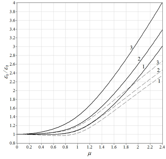
Figure 2. Ratio of lidar estimates of the dissipation rate by Methods 1 and 2 (${\epsilon }_1/{\epsilon }_2$) as a function of the ratio of the mean wind velocity to the linear scanning speed ($\mu$) at an elevation angle of 16° (curves 1), 35.3° (curves 2) and 60° (curves 3) and $\Delta y$ = 3 m (solid curves) and 12 m (dashed curves).

Equations (5)–(13) were used for analysis of the results obtained in experiments on the study of turbulence in the atmospheric boundary layer and were verified in the special experiment.

3. Experiment 2018

The experiment was conducted on 6–24 July 2018, at the Basic Experimental Observatory (BEO) of the Institute of Atmospheric Optics SB RAS in Tomsk, Russia (56°06′51.41″N, 85°06′03.22″E), with the Stream Line PCDL. In this experiment, the scanning was carried out at two alternative elevation angles: $\phi$ = ${\phi }_1$ = 35.3° and $\phi$ = ${\phi }_2$ = 60° [19]. The turbulence energy dissipation rate was estimated in this experiment by Method 1 [14] from the azimuth structure function, calculated for horizontal separations $l\Delta y<L_V$ not exceeding the integral scale of turbulence, which corresponds to the inertial subrange of turbulence. In this case, according to the Kolmogorov–Obukhov hypotheses, estimates of the dissipation rate calculated from lidar measurements at different elevation angles $\epsilon ({\phi }_1)$ and $\epsilon ({\phi }_2)$ for the same height should coincide. However, this turned out to not quite be the case. In the atmospheric layer at heights of 200–300 m (see Figure 5b in authors’ work [18]), the estimates $\epsilon ({\phi }_1)$ and $\epsilon ({\phi }_2)$ differed little on average. However, at heights below 150 m, $\epsilon ({\phi }_2)$ far exceeded $\epsilon ({\phi }_1)$.

The estimates of the dissipation rate in the authors’ work [19] were obtained by Method 1 [14], where the transport of turbulent inhomogeneities by the mean wind is neglected. Therefore, this neglect may be a possible reason for an excess of $<\epsilon ({\phi }_2)>$ over $<\epsilon ({\phi }_1)>$ at small heights $h$, where the speed of motion of the probing volume during the conical scanning at an elevation angle of 60° can be far smaller than the mean wind velocity. To check this hypothesis, we took the raw data measured by the lidar from 19:40 local time (LT) on 23 July 2018 to 08:20 LT on 24 July 2018, at elevation angles φ₁ = 35.3° and ${\phi }_2$ = 60° at the height $h$ = 70 m. In the experiment in the authors’ work [19], the duration of one scan $T_{\mathrm{scan}}$ was 60 s. At this scan duration, the speed of motion of the probing volume $V_s$ (Equation (3)) at a height of 70 m was 10.4 m/s and 4.2 m/s at elevation angles of 35.3° and 60°, respectively.

With regard to the short time δt ≈ 1 s needed for alternation of the elevation angle between 35.3° and 60°, the duration of one cycle $T_{\mathrm{circl}}=2(T_{\mathrm{scan}}+\delta t)$ in the experiment [19] exceeded 2 min by a little. The azimuth resolution was Δθ = 360°/M = 3°, where $M=T_{\mathrm{scan}}/\Delta t$ = 120 is the number of radial velocity estimates for one scan, $\Delta t=N_a/f_p$ = 0.5 s is the time of measurement for estimation of the radial velocity for every azimuth angle, $N_a$ = 7500 is the number of laser shots used for the raw data accumulation, and $f_p$ = 15 kHz is the pulse repetition frequency for the Stream Line lidar. From the lidar measurements at these parameters, we calculated the mean wind velocity $U({\phi }_1)$ and $U({\phi }_2)$ by the sine-wave fitting and the dissipation rate $\epsilon ({\phi }_2)$ and $\epsilon ({\phi }_1)$ by Methods 1 and 2 using Equations (1), (2) and (5)–(13). We used $N$ = 20 scans to estimate the mean velocity and the azimuth structure function by Equation (2). The duration of the measurements at two alternative elevation angles was a little longer than 40 min. Since Δθ = 3°, we took $l$ = 3 in Equation (5). For the mean velocity, we obtained practically coinciding estimates for U(φ₁) and $U({\phi }_2)$.

Figure 3 depicts the time series of the velocity ratio $\mu ({\phi }_i)=U({\phi }_i)/V_s({\phi }_i)$ and turbulence energy dissipation rate $\epsilon ({\phi }_i)$ calculated by Methods 1 and 2 for elevation angles of 35.3° ($i$ = 1) and 60° ($i$ = 2) at the height h = 70 m. It can be seen that, at an elevation angle of 35.3°, the parameter $\mu$ ranges from 0.5 to 0.8. According to curve 2 in Figure 2, the results of estimation of the dissipation rate by Methods 1 and 2 should not differ widely in this case. At an elevation angle of 60°, the parameter $\mu$ exceeds unity and can achieve 1.9. In this case, according to curve 2 in Figure 2, Method 1 can overestimate the dissipation rate by more than double. Figure 3b confirms this conclusion. If Method 2 is used, the estimates of the dissipation rate at elevation angles of 35.3° and 60° coincide on average (see Figure 3c). This fact indicates indirectly the applicability of Method 2 for determination of the turbulence energy dissipation rate from measurements by a conically scanning lidar at an arbitrary ratio between the mean wind velocity and the linear speed of motion of the probing volume.

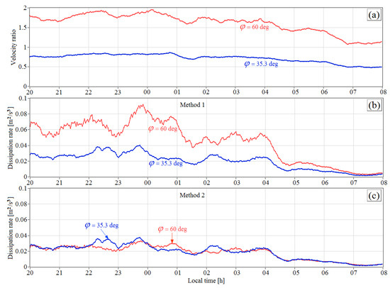
Figure 3. Time series of the ratio of the mean wind velocity to the linear scanning speed $\mu$ (a) and estimates of the turbulent energy dissipation rate obtained by Methods 1 (b) and 2 (c) at a height of 70 m. Scanning at an elevation angle of 35.3° (blue curves) and 60° (red curves). Measurements were taken at the BEO from 19:40 LT of 23 July 2018 to 08:20 LT of 24 July 2018.

4. Experiment 2019

The lidar experiment on the study of turbulence of the statically stable boundary layer was conducted in the coastal zone at the western coast of Lake Baikal near Listvyanka (52°50′47″N, 104°53′31″E) on 7–24 August of 2019. During this experiment, the Stream Line PCDL was installed at the territory of the Baikal Astrophysical Observatory of the Institute of Solar-Terrestrial Physics SB RAS, a few tens of meters from the building of the Big Solar Vacuum Telescope at a height of 180 m above the Baikal level, with a minimal separation of 340 m from the lake (see Figure 4 in authors’ work [15]). A sonic anemometer AMK-03 (Sibanalitpribor, Tomsk, Russia) with a sampling rate of 80 Hz was installed 50 m from the lidar at the top of a mast, at a height of 15 m above the lidar level. The lidar measurements were conducted with conical scanning at the elevation angle $\phi$ = 60°. The scanning duration and the azimuth resolution were the same as in experiment 2018 and amounted to $T_{\mathrm{scan}}$ = 1 min and $\Delta \theta$ = 3°, respectively.

In the experiment, a part of the lidar data was obtained under strong wind in the lower 100 m of the atmospheric layer above the lidar level. In particular, from 20:00 LT of 19 August to 02:30 LT of 20 August, the measurements were conducted at mean wind velocity U at a height of 55 m, ranging from 8 m/s to 12.7 m/s. The linear speed of the probing volume motion at a height of 55 m in the case of scanning at an elevation angle of 60° is $V_s$ = 3.3 m/s. We used these data to check Method 2 in terms of its estimation of the turbulence energy dissipation rate. To obtain estimates of the mean velocity and the dissipation rate ${\epsilon }_1$ and ε₂ (respectively, by Methods 1 and 2) by Equation (9), in Equations (1) and (2), we set $N$ = 30 consecutive scans (30 min average). The same 30 min average was applied to obtain estimates of the mean wind velocity and the turbulent energy dissipation rate from measurements of the sonic anemometer. We obtained dissipation rate estimates ${\epsilon }_s$ from temporal structure function $D_{\parallel }(U\tau )$ of the longitudinal component of the wind velocity vector measured by the sonic anemometer, where 1 s $\le \tau \le$ 3 s, with the use of Taylor’ hypothesis of “frozen” turbulence (see Equation (26) in authors’ work [14]). Figure 4 demonstrates the results obtained from the lidar measurements. One can see (Figure 3e) that the estimate ${\epsilon }_1$ can exceed the estimate ${\epsilon }_2$ by an order of magnitude.

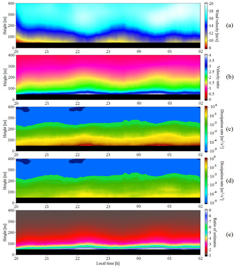
Figure 4. Height–temporal distributions of the mean wind velocity (a), ratio of the mean wind velocity to the linear scanning speed $\mu$ (b), estimates of the turbulent energy dissipation rate obtained by Methods 1 (c) and 2 (d) and the ratio of these estimates (e). Measurements were taken on the coast of Lake Baikal from 19:45 LT of 19 August to 02:15 LT of 20 August 2019.

Using the data from Figure 4a,b, we drew the vertical and temporal profiles of the mean wind velocity $U$ and the velocity ratio $\mu =U/V_s$, which are shown as solid curves in Figure 5. The dashed straight lines in this figure correspond to the linear scanning speed $V_s$ at different heights h. We can see that, in the 300 m layer adjacent to the ground, the parameter $\mu$ decreases with height despite an increase in the velocity $U$. Above $h$ = 300 m, this parameter takes on values at which the estimates of the dissipation rate ${\epsilon }_1$ and ${\epsilon }_2$ differ a little from each other. At the height h = 55 m, the parameter $\mu$ at its maximum approaches four (see the blue curve in Figure 5d), while ε₁ becomes an order of magnitude larger than ${\epsilon }_2$.

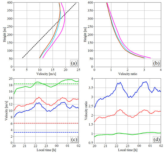
Figure 5. Vertical profiles (a,b) at 21:00 LT (brown curves), 23:00 LT (pale-blue curves) and 01:00 LT (pink curves) and time series (c,d) at a height of 55 m (blue curves), 100 m (red curves) and 300 m (green curves) for the mean wind velocity (a,c) and the ratio of the mean wind velocity to the linear speed of the probing volume motion $\mu$ (b,d). The data are taken from Figure 4. The dashed lines show the linear scanning speeds at the corresponding heights.

Figure 6 shows the time series of the dissipation rate estimates ${\epsilon }_1(t)$ and ${\epsilon }_2(t)$ obtained from lidar data with Methods 1 and 2, respectively, at heights of 55 m and 100 m, along with ${\epsilon }_s(t)$ calculated from the data measured by the sonic anemometer at a height of 15 m. One can see that if the transport of turbulent inhomogeneities by the mean wind is neglected (Method 1), then the estimates ${\epsilon }_1(t)$ at a height of 100 m are close to the estimates ${\epsilon }_s(t)$ at a height of 15 m, while those at a height of 55 m exceed by approximately five times the estimates obtained from the sonic anemometer measurements at a height of 15 m. Although the measurements were conducted under strong wind and intense turbulence, the estimates ${\epsilon }_1\sim$1 m²/s³ obtained from the lidar data at a height of 55 m and ${\epsilon }_1\sim$0.2 m²/s³ at a height of 100 m are obviously overestimated.

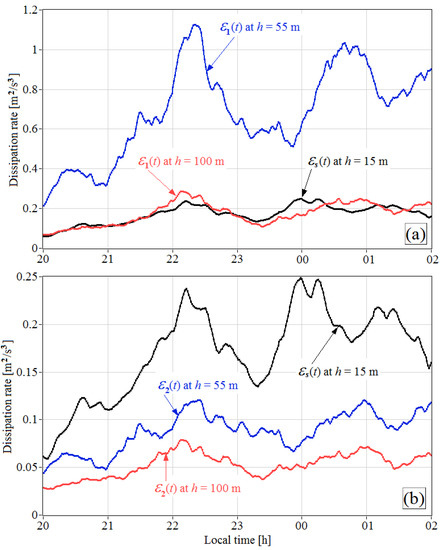
Figure 6. Time series of the turbulent energy dissipation rate as estimated from the data of the sonic anemometer at a height of 15 m (black curves) and the lidar at a height of 55 m (blue curves) and 100 m (red curves). The lidar estimates of the dissipation rate are obtained with Method 1 (a) and Method 2 (b). The lidar data are taken from Figure 4c,d.

The use of Method 2 for estimation of the dissipation rate from the lidar data provides the more likely result (Figure 6b). At heights of 55 m and 100 m, the dissipation rate takes on smaller values than those calculated for the height h = 15 m from the sonic anemometer data. They decrease with height and are comparable in terms of the absolute value with the known experimental data (see, for example, [20,21]).

The vertical profiles of the estimates of the turbulent energy dissipation rate obtained from the lidar data with Methods 1 and 2 are shown in Figure 7 as green and blue curves, respectively. It can be seen from Figure 7e that, at a height of 55 m, the estimate ${\epsilon }_1$ is ten times larger than the estimate ${\epsilon }_2$. Red squares indicate the estimates of the dissipation rate from measurements by the sonic anemometer at a height of 15 m. In this experiment, the minimum height of measurement by the lidar is $h_0\approx$ 55 m and the height step is $\Delta h\approx$ 15 m. To compare the estimates of the dissipation rate ${\epsilon }_2(h_s)$ (Method 2) and ${\epsilon }_s$ obtained from measurements, respectively, with the lidar and sonic anemometer at a height of $h_s$ = 15 m, we used the extrapolation of the height profile ${\epsilon }_2(h_k)$ ($h_k=h_0+k\Delta h$; $k=0,1,2,3$) from the layer of 55–100 m to the height h_s as follows. First, for each vertical profile ${\epsilon }_2(h_k)$ shown in Figure 7 within the layer 55–100 m, we used a linear fitting of $\lg \left({\overline{\epsilon }}_2(h_k)\right)=\alpha h_k+\beta$, where $\alpha$ is the slope and $\beta$ is the intercept, to lg(ε₂(h_k)), by the least squares method. We then calculated values ${\overline{\epsilon }}_2(h_s)$ for the height of the sonic anemometer position. In Figure 7, in the 15–100 m layer, the dashed lines show the profiles ${\overline{\epsilon }}_2(h)$, where $h\in [h_s,h_3]$. Calculations of the value $|{\overline{\epsilon }}_2(h_s)/{\epsilon }_s-1|\times 100\%$ showed that it does not exceed 20%. Thus, if, in the 15–100 m layer, the vertical profile $\lg \left({\epsilon }_2(h)\right)$ has a height dependence which is close to linear, the lidar estimates of the dissipation rate obtained by Method 2 are in good agreement with the results of measurements with the sonic anemometer (at least, the discrepancy of the results are within the statistical error, examples of which are given below).

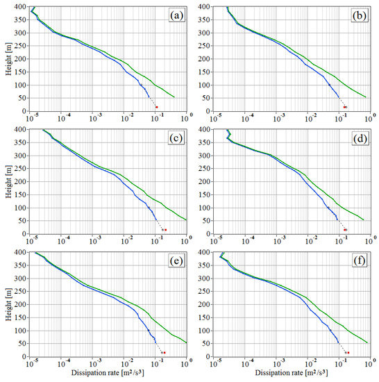
Figure 7. Vertical profiles of the turbulent energy dissipation rate at 20:30 (a), 21:30 (b), 22:30 (c), 23:30 (d) on 19 August and 00:30 (e) and 01:30 (f) on 20 August 2019, as calculated with Method 1 (green curves) and Method 2 (blue curves). The lidar data are taken from Figure 4c,d. Red squares indicate estimates of the dissipation rate from simultaneous measurements by the sonic anemometer.

5. Experiment 2020

An experiment focusing on the testing of Method 2 for estimation of the turbulent energy dissipation rate from the data measured by a conically scanning PCDL was carried out in May 2020 at the territory of the BEO. Continuous lidar measurements were performed in two stages: (1) from 10 to 15 May and (2) from 19 to 26 May 2020. The results of estimation of the dissipation rate by Methods 1 and 2 in the experiment were compared with the estimates $\epsilon$ from the data of the sonic anemometer AMK-03 with sampling rate of 80 Hz (Sibanalitpribor, Tomsk, Russia), installed on a 43 m tower with boom length of 2 m at a height of 42 m. The separation between the Stream Line lidar and the tower was 160 m.

The elevation angle $\phi$ was set equal to 16° in the measurements, so that the center of probing pulses achieved the height $h$ = 42 m at the distance $R$ = 152 m from the lidar. At a height of 42 m, the radius and the length of the scanning circle were R′ = Rcosφ = 146 m and $L_c=2\pi R^{\prime }$ = 918 m, respectively. The scan duration $T_{\mathrm{scan}}$ was set to 5 min. The linear speed of motion of the probing volume along the scanning circle $V_s=L_c/T_{\mathrm{scan}}$ was $\approx$3 m/s. To estimate one value of the radial velocity, $N_a$ = 15,000 laser shots were used for the raw data accumulation, so that the duration of measurement for every azimuth angle was $\Delta t=N_a/f_p$ = 1 s. For one scan, we obtained $M=T_{\mathrm{scan}}/\Delta t$ = 300 estimates of the radial velocity at different azimuth angles (300 rays), with the resolution $\Delta \theta$ = 360°/M = 1.2° and the distance between them along the circle (between centers of probing volumes) $\Delta y=\Delta \theta R^{\prime }\approx$ 3 m.

To obtain estimates of the mean wind velocity and the dissipation rate ε₁ and ${\epsilon }_2$ (by Methods 1 and 2, respectively) using Equation (9), for the averages in Equations (1) and (2), we used $N$ = 7 consecutive scans (approximately 35 min average). In Equation (9), we took $l$ = 3. The estimates of the dissipation rate ${\epsilon }_s$ from measurements by the sonic anemometer were determined from temporal spectra of the longitudinal (along the mean wind direction) component of the wind vector within the inertial subrange from 0.2 to 2 Hz, where the spectrum was characterized by the “-5/3” power dependence on frequency, with the use of Taylor’s “frozen” turbulence hypothesis. In addition, the dissipation rate was estimated with the use of the time series of the wind velocity measured by the sonic anemometer for 35 min.

However, we were able to use the data of the sonic anemometer measured only at a certain interval of wind direction angles, due to the distortions (shading) introduced by the mast. Therefore, in the first part of the experiment (from 10 May to 15 May), only those raw data of the sonic anemometer were suitable for further processing, and these were measured within a period of 17.5 h, starting at 07:40 local time on 13 May 2020.

Figure 8 exemplifies the time series of the mean wind velocity obtained from measurements by the lidar U and by the sonic anemometer $U_s$ for 17.5 h starting from 07:40 LT on 13 May 2020. One can see that approximately half of the time, the mean wind velocity $U$ ($U_s$) exceeded the linear speed of motion of the probing volume $V_s$ = 3 m/s. It can be seen that the greatest difference between the estimates of the dissipation rate by Methods 1 and 2 was observed at $\mu >2$, which is in agreement with the calculated results shown in Figure 2. It follows that the estimates of the dissipation rate obtained by Method 2 from the lidar data and from the sonic anemometer data are in good agreement at all values of the velocity ratio $\mu$ given in Figure 8a. The application of Method 1 would lead to a threefold overestimation of the dissipation rate at 17:00 LT.

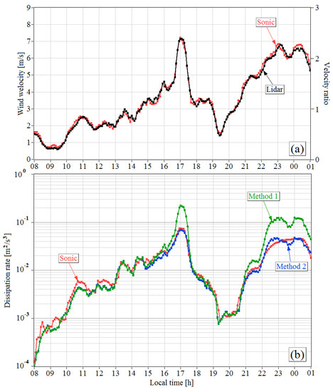
Figure 8. Time series of the mean wind velocity and the velocity ratio $\mu$ (a), the turbulence energy dissipation rate (b) at a height of 42 m as obtained from measurements by the Stream Line lidar (black, green and blue curves) and the sonic anemometer (red curves). The measurements were carried out at the BEO starting from 08:00 LT on 13 May of 2020. For estimation of the dissipation rate, Method 1 (green curve) and Method 2 (blue curve) were used.

Using the data of Figure 8, we compared the estimates of the mean wind velocity and the dissipation rate from simultaneous measurements by the sonic anemometer ($U_s$ and ε_s) and the lidar ($U$ and ${\epsilon }_2$). The results of this comparison are shown in Figure 9. On the assumption of statistical independence of the estimates and equal errors in estimation of the mean wind velocity from lidar data $U$ and from sonic anemometer data $U_s$, as well as statistical independence of the estimates and equal errors in estimation of the dissipation rate ${\epsilon }_2$ and ${\epsilon }_s$, we calculated the relative bias $B_U=<{\eta }_U{>}_p\times 100\%$ and the relative error $E_U=\sqrt{(<{\eta }_U^2{>}_p-<{\eta }_U{>}_p^2)/2}\times 100\%$ of estimation of the wind velocity along with the relative bias $B_{\epsilon }=<{\eta }_{\epsilon }{>}_p\times 100\%$ and the relative error $E_{\epsilon }=\sqrt{(<{\eta }_{\epsilon }^2{>}_p-<{\eta }_{\epsilon }{>}_p^2)/2}\times 100\%$ of estimation of the dissipation rate. The operator $<\dots {>}_p$ means an average over all pairs of estimates ($U$, $U_s$) or (ε₂, ε_s), where $p$ is the number of such pairs. To calculate ${\eta }_U=(U-U_s)/[(U+U_s)/2]$ and η_ε = (ε₂ − ε_s)/[(ε₂ + ε_s)/2], we used the data of Figure 9a,b, respectively. Thereby, from the data of Figure 9, we obtained $B_U$ = −2%, E_U = 4%, $B_{\epsilon }$ = −9%, and E_ε = 14%.

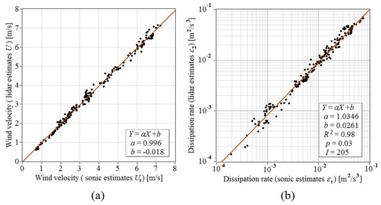
Figure 9. Comparison of the estimates of the mean wind velocity (a) and turbulent energy dissipation rate (b) obtained from simultaneous measurements by the lidar (vertical axes) and the sonic anemometer (horizontal axes). The data are taken from Figure 8. In (a,b), the brown line is the best fit given by equation $Y_i=a{X}_i+b$, where $X_i=U_s$ (a) and $X_i=\lg ({\epsilon }_s)$ (b).

Using data from Figure 9b, we found that the coefficient of correlation between log(ε_s) and log(ε₂) equals 0.987; the results of linear regression are $a$ = 1.0346 and $b$ = 0.0261 ($Y_i=a{X}_i+b$, where X_i = lg(ε_s), $Y_i=\lg ({\epsilon }_2)$, $i=1,2,3,\dots ,I$, $I$ = 205, $a$ and b are the slope and intercept of this linear equation); the coefficient of determination $R^2$ = 0.98 and p-value as a measure of statistical significance equals 0.03.

In the second part of the experiment (measurements from 19 May to 26 May 2020), the wind direction was continuous for 62 h so that there was no distortion of the wind data due to “shading” by the mast on which the sonic anemometer was installed. Consequently, we were able to compare the results of measurements by the lidar and sonic anemometer for this period of time.

Figure 10 depicts the 62 h time series of the ratio $\mu$ of the mean wind velocity to the linear speed of the probing volume and the estimates of the dissipation rate from the measurements by the sonic anemometer and the lidar starting from 16:00 LT on 20 May of 2020. It can be seen that, at $\mu >1$, Method 1 markedly (up to 2.7 times) overstates the dissipation rate in comparison with ${\epsilon }_2$ and ε_s.

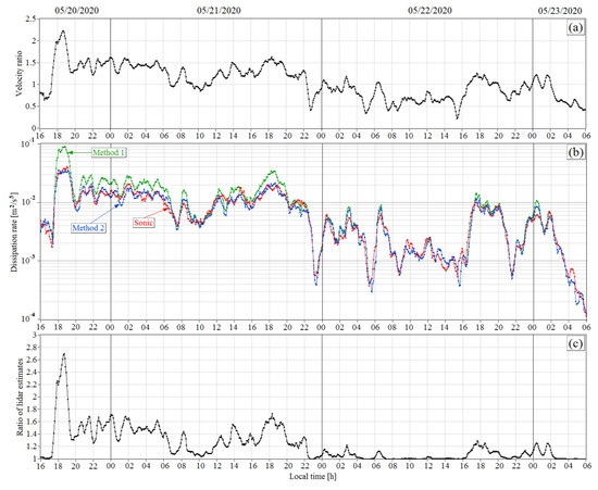
Figure 10. Time series at a height of 42 m for (a) the ratio $\mu$ of the mean wind velocity to the linear speed of motion of the probing volume, (b) the turbulence energy dissipation rate calculated from lidar data by Method 1 (green curve) and Method 2 (blue curve) and from data of sonic anemometer (red curve) and (c) the ratio of lidar estimates of the dissipation rate calculated by Methods 1 and 2. Measurements at the BEO started from 16:00 LT on 20 May of 2020.

Using the data of Figure 10b, we compared the estimates of the dissipation rate obtained from measurements by the sonic anemometer ${\epsilon }_s$ with the lidar estimates ${\epsilon }_1$ and ${\epsilon }_2$. The results of the comparison are shown in Figure 11. It can be seen from Figure 11a that, at strong turbulence, (when ${\epsilon }_s\ge$ 10⁻² m²/s³) and $\mu >1$, the lidar estimates of the dissipation rate ε₁, on average, exceed the estimates ${\epsilon }_s$ obtained from measurements by the sonic anemometer. Under the same conditions, the difference between the estimates ε₂ and ${\epsilon }_s$ (Figure 11b) is much smaller.

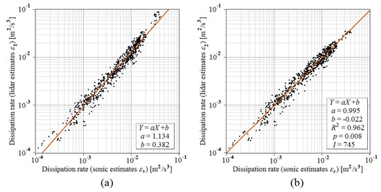
Figure 11. Comparison of estimates of the turbulence energy dissipation rate obtained from simultaneous measurements by the lidar (vertical axes) and the sonic anemometer (horizontal axes). Lidar estimates of the dissipation rate were obtained with Methods 1 (a) and 2 (b). The data are taken from Figure 10b. In (a,b), the brown line is the best fit given by equation Y_i = aX_i + b, $X_i=\lg ({\epsilon }_s)$.

The relative bias of estimates of the dissipation rate calculated by Methods 1 and 2 as judged from the data of Figure 11 is, respectively, $B_{\epsilon }$ = 15% and $B_{\epsilon }$ = −2%. This result allows us to assert that Method 2 gives an unbiased estimate of the dissipation rate at an arbitrary ratio of the mean wind velocity to the linear speed of conical scanning. According to the data of Figure 11, the relative statistical errors of the lidar estimates ${\epsilon }_1$ and ${\epsilon }_2$ differ less widely, at $E_{\epsilon }$ = 20% and $E_{\epsilon }$ = 16%, respectively. Parameters of the linear regression, including the slope $a$ and the intercept $b$ (equal to 1.134 and 0.382 in the case of Method 1 (Figure 11a; in this case, for calculation of a and b, we used lg(ε₁) instead of $\lg ({\epsilon }_2)$) and 0.996 and −0.026 in the case of Method 2 (Figure 11b). The coefficient of the correlation between lg(ε_s) and $\lg ({\epsilon }_2)$ equals 0.98. Using data from Figure 11b, we determined that the coefficient of determination $R^2$ = 0.962 and p-value as a measure of statistical significance equals 0.008.

Thus, the comparative analysis of the results of measurements by a conically scanning lidar and a sonic anemometer at the same height, carried out in this section, showed that taking into account the transfer of turbulent inhomogeneities by the mean wind (Method 2) makes it possible to obtain unbiased lidar estimates of the dissipation rate at arbitrary values of parameter $\mu$.

It should be noted that the results presented in Figure 3 (experiment 2018), Figure 4 (experiment 2019) and Figure 8 and Figure 10 (experiment 2020) were obtained from lidar measurements at relatively large signal-to-noise ratios $\mathrm{SNR}$ (the ratio of the mean power of the lidar echo signal to the mean power of the detector noise in the receiver passband of 50 MHz). Consequently, the instrumental error in estimating the radial velocity ${\sigma }_e$, which substantially depends on $\mathrm{SNR}$ and $N_a$, should be small, and this error should insignificantly affect the accuracy of the estimate of the turbulent energy dissipation rate. Therefore, in the experiments of 2018 ($N_a$ = 7500) and 2020 ($N_a$ = 15,000), the signal-to-noise ratio varied from −10 dB to 0 dB and the error ${\sigma }_e$ did not exceed 0.1 m/s (σ_e was calculated by Equation (23) in authors’ work [14] after replacing $A(l\Delta y)$ with $A_2(l\Delta y)$), and in the 2019 experiment ($N_a$ = 7500), it varied from −13 dB to −8 dB and ${\sigma }_e\le$ 0.2 m/s.

6. Discussion

Pulsed coherent Doppler lidars capable of measuring the radial velocity with high spatial and temporal resolution [1,2,22] are effective technical means of obtaining information on the turbulent energy dissipation rate in the atmospheric boundary layer (in particular, the Stream Line lidar used in this work). The method developed in the authors’ work [14] for retrieving the vertical profiles of the dissipation rate from measurements with a conically scanning PCDL has a number of advantages over the previously used approaches [4,5,6,7,8,9,10,11,12]. In particular, it allows one to take into account the effect of averaging the radial velocity over the probing volume. However, the application of this method assumes a significant excess of the linear speed of the conical scanning $V_s$ over the average wind velocity $U$ (i.e., $\mu =U/V_s<<1$), which is not always the case in practice. Indeed, if the dissipation rate is determined from measurements at the height of the atmospheric surface layer at a relatively large elevation angle $\phi$ and, moreover, with a strong wind, then parameter $\mu$ can be many times greater than unity. In this case, the distribution of the radial velocity within the probing volume will change with time, mainly due to the transfer of turbulent inhomogeneities by the mean wind and not due to the movement of the probing volume around the base of the scanning cone.

To obtain an estimate of the dissipation rate (using Equation (9)) from the lidar measurements of the azimuth structure function of the radial velocity at any velocity ratio $\mu$, it is necessary to know the equation for the function $A_2(l\Delta y)$, which would take into account (1) the motion of the probing volume (on the horizontal plane) during conical scanning, (2) wind transfer of turbulent inhomogeneities and (3) averaging of the radial velocity over the probing volume. In this work, using Taylor’s hypothesis of “frozen” turbulence and a number of approximations (see the derivation of the equation in Appendix A), we obtained an equation for the function $A_2(l\Delta y)$, taking into account all these three factors (see Equations (10)–(13)). To test this method (Method 2, in which the function $A_2(l\Delta y)$ is used in Equation (9)), we used the data of lidar experiments, in which any values of the parameter $\mu$ were realized, including $\mu >>1$.

Testing of Method 2 in the 2018 experiment (see Section 3) showed that the reason for the discrepancy in the estimates of the turbulent energy dissipation rate from the measurements by the Stream Line lidar in the atmospheric surface layer at different elevation angles (${\phi }_1$ = 35.3° and ${\phi }_2$ = 60°) is that the method used in the authors’ work [19] (Method 1) does not take into account the transfer of turbulent inhomogeneities by the mean wind. The use of Method 2 made it possible to obtain similar results from lidar measurements at angles ${\phi }_1$ and ${\phi }_2$.

The use (along with the Stream Line lidar) of sonic anemometers in the 2019 (Section 4) and 2020 (Section 5) experiments made it possible to compare the estimates of the dissipation rate from the measurements by the lidar (estimates ${\epsilon }_1$ and ${\epsilon }_2$ obtained by Methods 1 and 2, respectively) and the sonic anemometer (estimate ${\epsilon }_s$). Since, in the 2019 experiment, the height of the sonic anemometer position was 40 m less than the minimum height of the lidar measurement, to compare the estimates of the dissipation rate, we used the extrapolation of the vertical profile ${\epsilon }_2(h)$ to the level of the sonic anemometer and also obtained good agreement between the results, including the case at $\mu >>1$ (see Figure 7). The 2020 experiment, whose data we used to directly compare the dissipation rate estimates from measurements with a lidar and a sonic anemometer at the same height, convincingly proved the applicability of Method 2 for any values of parameter $\mu$.

It is worth using the generalized method at both large wind velocities and small probing heights, up to 200–300 m. At heights above the surface atmospheric layer, the method in the authors’ work [14] usually provides quite acceptable (in accuracy) estimates of the dissipation rate. Its application does not require complicated calculations in contrast to the generalized method (compare Equation (20) in [14] with Equations (10)–(13) of this paper).

7. Conclusions

The equation for the azimuth structure function of fluctuations of the radial velocity measured by PCDL, with regard to the transport of turbulent inhomogeneities by the mean wind, was derived based on Taylor’s hypothesis of “frozen” turbulence. With this equation, the method of azimuth structure function for estimation of the turbulence energy dissipation rate [14,19,23] was generalized to the case of an arbitrary ratio between the wind velocity and the linear speed of motion of the probing volume during the scanning process. The limits of applicability of the method of azimuth structure function [14] were determined. It has been shown that this method [14] overestimates the dissipation rate, starting from the ratio $\mu$ of the mean wind velocity to the linear scanning speed ranging within 0.55–1.1, depending on the elevation angle and the separation $\Delta y$ between the centers of neighboring probing volumes on the circle of the scanning cone base.

The generalized method was tested with the data of field experiments with the Stream Line lidar and the sonic anemometer. It was shown that the generalized method provides a practically unbiased estimate of the dissipation rate at an arbitrarily large ratio $\mu >>1$, whereas the method from the authors [14] overestimates the dissipation rate by an order of magnitude at $\mu ~4$.

References

- Pearson, G.; Davies, F.; Collier, C. An analysis of performance of the UFAM Pulsed Doppler lidar for the observing the boundary layer. J. Atmos. Ocean. Technol. 2009, 26, 240–250. [Google Scholar] [CrossRef]
- Vasiljevic, N.; Lea, G.; Courtney, M.; Cariou, J.P.; Mann, J.; Mikkelsen, T. Long-Range Wind Scanner System. Remote Sens. 2016, 8, 896. [Google Scholar] [CrossRef]
- Eberhard, W.L.; Cupp, R.E.; Healy, K.R. Doppler lidar measurement of profiles of turbulence and momentum flux. J. Atmos. Ocean. Technol. 1989, 6, 809–819. [Google Scholar] [CrossRef]
- Frehlich, R.G.; Hannon, S.M.; Henderson, S.W. Coherent Doppler lidar measurements of wind field statistics. Bound.-Layer Meteorol. 1998, 86, 223–256. [Google Scholar] [CrossRef]
- Smalikho, I.; Köpp, F.; Rahm, S. Measurement of atmospheric turbulence by 2-μm Doppler lidar. J. Atmos. Ocean. Technol 2005, 22, 1733–1747. [Google Scholar] [CrossRef]
- Frehlich, R.G.; Meillier, Y.; Jensen, M.L.; Balsley, B.; Sharman, R. Measurements of boundary layer profiles in urban environment. J. Appl. Meteorol. Climatol. 2006, 45, 821–837. [Google Scholar] [CrossRef]
- Banta, R.M.; Pichugina, Y.L.; Brewer, W.A. Turbulent velocity-variance profiles in the stable boundary layer generated by a nocturnal low-level jet. J. Atmos. Sci. 2006, 63, 2700–2719. [Google Scholar] [CrossRef]
- O’Connor, E.J.; Illingworth, A.J.; Brooks, I.M.; Westbrook, C.D.; Hogan, R.J.; Davies, F.; Brooks, B.J. A method for estimating the kinetic energy dissipation rate from a vertically pointing Doppler lidar, and independent evaluation from balloon-borne in situ measurements. J. Atmos. Ocean. Technol. 2010, 27, 1652–1664. [Google Scholar] [CrossRef]
- Sathe, A.; Mann, J. A review of turbulence measurements using ground-based wind lidars. Atmos. Meas. Tech. 2013, 6, 3147–3167. [Google Scholar] [CrossRef]
- Sathe, A.; Mann, J.; Vasiljevic, N.; Lea, G. A six-beam method to measure turbulence statistics using ground-based wind lidars. Atmos. Meas. Tech. Discuss. 2014, 7, 10327–10359. [Google Scholar] [CrossRef]
- Newman, J.F.; Klein, P.M.; Wharton, S.; Sathe, A.; Bonin, T.A.; Chilson, P.B.; Muschinski, A. Evaluation of three lidar scanning strategies for turbulence measurements. Atmos. Meas. Tech. 2016, 9, 1993–2013. [Google Scholar] [CrossRef]
- Bonin, T.A.; Choukulkar, A.; Brewer, W.A.; Sandberg, S.P.; Weickmann, A.M.; Pichugina, Y.L.; Banta, R.M.; Oncley, S.P.; Wolfe, D.E. Evaluation of turbulence measurement techniques from a single Doppler lidar. Atmos. Meas. Tech. 2017, 10, 3021–3039. [Google Scholar] [CrossRef]
- Wildmann, N.; Bodini, N.; Lundquist, J.K.; Bariteau, L.; Wagner, J. Estimation of turbulence dissipation rate from Doppler wind lidars and in situ instrumentation for the Perdigão 2017 campaign. Atmos. Meas. Tech. 2019, 12, 6401–6423. [Google Scholar] [CrossRef]
- Smalikho, I.N.; Banakh, V.A. Measurements of wind turbulence parameters by a conically scanning coherent Doppler lidar in the atmospheric boundary layer. Atmos. Meas. Tech. 2017, 10, 4191–4208. [Google Scholar] [CrossRef]
- Banakh, V.A.; Smalikho, I.N. Lidar observations of atmospheric internal waves in the boundary layer of atmosphere on the coast of Lake Baikal. Atmos. Meas. Tech. 2016, 9, 5239–5248. [Google Scholar] [CrossRef]
- Smalikho, I.N.; Banakh, V.A.; Holzäpfel, F.; Rahm, S. Method of radial velocities for the estimation of aircraft wake vortex parameters from data measured by coherent Doppler lidar. Opt. Express 2015, 23, A1194–A1207. [Google Scholar] [CrossRef] [PubMed]
- Lhermitte, R.M.; Atlas, D. Precipitation motion by pulse Doppler. In Proceedings of the 9th Weather Radar Conference, Kansas City, MO, USA, 23–26 October 1961; pp. 218–223. [Google Scholar]
- Banakh, V.A.; Smalikho, I.N. Coherent Doppler Wind Lidars in a Turbulent Atmosphere; Artech House: Boston, MA, USA; London, UK, 2013; p. 248. ISBN 978-1-60807-667-3. [Google Scholar]
- Banakh, V.A.; Smalikho, I.N. Lidar estimates of the anisotropy of wind turbulence in a stable atmospheric boundary layer. Remote Sens. 2019, 11, 2115. [Google Scholar] [CrossRef]
- Lumley, J.L.; Panofsky, H.A. The Structure of Atmospheric Turbulence; Interscience Publishers: New York, NY, USA, 1964. [Google Scholar]
- Byzova, N.L.; Ivanov, V.N.; Garger, E.K. Turbulence in Atmospheric Boundary Layer; Gidrometeoizdat: Leningrad, Russia, 1989. [Google Scholar]
- Grund, C.J.; Banta, R.M.; George, J.L.; Howell, J.N.; Post, M.J.; Richter, R.A.; Weickman, A.M. High-resolution Doppler lidar for boundary layer and cloud research. J. Atmos. Ocean. Technol. 2001, 18, 376–393. [Google Scholar] [CrossRef]
- Banakh, V.A.; Smalikho, I.N.; Falits, A.V. Wind-Temperature Regime and Wind Turbulence in a Stable Boundary Layer of the Atmosphere: Case Study. Remote Sens. 2012, 12, 955. [Google Scholar] [CrossRef]
- Monin, A.S.; Yaglom, A.M. Statistical Fluid Mechanics, Volume II: Mechanics of Turbulence; M.I.T. Press: Cambridge, MA, USA, 1971. [Google Scholar]
© 2020 by the authors. Licensee MDPI, Basel, Switzerland. This article is an open access article distributed under the terms and conditions of the Creative Commons Attribution (CC BY) license (http://creativecommons.org/licenses/by/4.0/).