Challenges and Future Perspectives of Multi-/Hyperspectral Thermal Infrared Remote Sensing for Crop Water-Stress Detection: A Review

Abstract

Thermal infrared (TIR) multi-/hyperspectral and sun-induced fluorescence (SIF) approaches together with classic solar-reflective (visible, near-, and shortwave infrared reflectance (VNIR)/SWIR) hyperspectral remote sensing form the latest state-of-the-art techniques for the detection of crop water stress. Each of these three domains requires dedicated sensor technology currently in place for ground and airborne applications and either have satellite concepts under development (e.g., HySPIRI/SBG (Surface Biology and Geology), Sentinel-8, HiTeSEM in the TIR) or are subject to satellite missions recently launched or scheduled within the next years (i.e., EnMAP and PRISMA (PRecursore IperSpettrale della Missione Applicativa, launched on March 2019) in the VNIR/SWIR, Fluorescence Explorer (FLEX) in the SIF). Identification of plant water stress or drought is of utmost importance to guarantee global water and food supply. Therefore, knowledge of crop water status over large farmland areas bears large potential for optimizing agricultural water use. As plant responses to water stress are numerous and complex, their physiological consequences affect the electromagnetic signal in different spectral domains. This review paper summarizes the importance of water stress-related applications and the plant responses to water stress, followed by a concise review of water-stress detection through remote sensing, focusing on TIR without neglecting the comparison to other spectral domains (i.e., VNIR/SWIR and SIF) and multi-sensor approaches. Current and planned sensors at ground, airborne, and satellite level for the TIR as well as a selection of commonly used indices and approaches for water-stress detection using the main multi-/hyperspectral remote sensing imaging techniques are reviewed. Several important challenges are discussed that occur when using spectral emissivity, temperature-based indices, and physically-based approaches for water-stress detection in the TIR spectral domain. Furthermore, challenges with data processing and the perspectives for future satellite missions in the TIR are critically examined. In conclusion, information from multi-/hyperspectral TIR together with those from VNIR/SWIR and SIF sensors within a multi-sensor approach can provide profound insights to actual plant (water) status and the rationale of physiological and biochemical changes. Synergistic sensor use will open new avenues for scientists to study plant functioning and the response to environmental stress in a wide range of ecosystems.

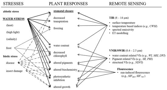
1. Importance of Water-Stress Detection

Water-deficit stress, usually shortened to water or drought stress, describes the plant physiological responses induced by a lack of available water due to either soil water deficit or high evaporative demand of the atmosphere. Water stress induces dehydration in the plant and prevents plant cells from keeping water concentrations at an acceptable and healthy level [1,2]. Therefore, water stress is one of the most critical abiotic stressors limiting plant growth, crop yield and quality concerning food production [3,4].

Since the global population is projected to grow by about 2.3 billion people between 2015 and 2050 and societies are changing from low to medium per capita income, global food demand is expected to double within the same time [5,6,7]. Therefore, one of the most challenging tasks of our generation is to meet the second Sustainable Development Goal as defined in the 2030 agenda for sustainable development by the United Nations: “End hunger, achieve food security and improved nutrition and promote sustainable agriculture” [8]. In this respect, agricultural processes need to be optimized and innovative farming methods must be developed to guarantee global food supply, as arable land and environmental resources have almost reached the limits of sustainability.

Water is the most valuable resource of our planet. Presently, agriculture consumes 80–90% of the freshwater used by humans worldwide and about two thirds of this freshwater is required for crop irrigation [9]. Therefore, the ultimate goal must be a reduction in the amount of water used per unit yield [10].

In addition, anthropogenic climate change is predicted to cause an increase of 1.0–2.5 °C in the annual mean global temperature over the next 50 years with a tremendous impact on agriculture [11]. Consequently, evapotranspiration (ET) rates will increase and thus, the demand of water for crop irrigation will further rise. At the same time, extreme weather events such as droughts will appear more frequently and be more severe. These facts add some extra pressure to increasing global water scarcity and the need for saving water.

Hence, it is desired to reduce the amount of water used per unit yield by reducing yield loss and by reducing the amount of water used for irrigation. To achieve this goal, early detection and monitoring of plant responses to water stress in agricultural crops are mandatory. Remote sensing offers the opportunity to acquire high spatial, spectral and temporal resolution data as input for precision agriculture [12]. Precision agriculture promises great potential to close the yield gap by optimizing food production using the right management practice at the right place and the right time while keeping the consumption of resources at an environmentally sustainable level [13].

2. Plant Responses to Water Stress

Plant responses to water stress are numerous and complex (see [4,14,15,16] for comprehensive reviews). They appear synergistically or antagonistically and are modified by co-occurring plant stresses under field conditions (Figure 1) [4,17,18]. Therefore, it remains difficult to detect and monitor plant water deficit based on a single plant response [19]. In general, water deficit causes physiological and biochemical changes which induce a reduction in photosynthesis and thus plant growth [16]. However, the timing, intensity, and duration of water stress are crucial to determine the plant physiological responses and their impact on plant metabolism [20]. For example, under mild water-stress conditions, plant regulation of water loss and uptake still allows the plant to maintain relative leaf water content with no or only little change in photosynthetic capacity. In contrast, severe water deficit induces serious physiological and biochemical changes, which lead to effects ranging from inhibition of photosynthesis and growth to leaf wilting and the loss of key pigments such as chlorophyll and thus to irreversible damages to the photosynthetic machinery [15,16,17]. Hence, plants have developed multiple mechanisms to prevent severe damage through water stress [21].

The first plant response to water stress is stomatal closure, which prevents transpirational water loss (e.g., [4,15,17]). In particular, stomatal closure is the response to either a deficit in soil water supply or to low-humidity atmosphere with high evaporative demand. It is commonly assumed that stomatal response is rather linked to soil water content than to leaf water content. This suggests that stomata are most likely triggered by chemical signals, such as the accumulation of abscisic acid (ABA) in dehydrated roots rather than by a reduced cell turgor [4]. However, under severe and/or prolonged water stress, cell turgor, and leaf water content is also reduced [15]. As a consequence, the exchange of water vapor between plants and atmosphere is reduced by stomatal closure and thus, the evaporative cooling effect is decreased resulting in an overall increase of plant surface temperature compared to a plant which does not suffer from water stress [14,18,22].

However, the stomata not only control plant transpiration but also plant respiration which inhibits CO₂ uptake and fixation. As a result of stomatal closure, the photosynthetic rate is reduced, which causes a reduction in cell division and thus slows down leaf growth and reduces the rate of leaf surface area expansion. A persistent water deficit will further damage the photosynthetic machinery through loss of chlorophyll, which finally introduces changes in leaf color and wilting [15,16,20]. Another plant response to water stress is the change in sun-induced fluorescence (SIF). While the photosynthetic rate is reduced by a decreased CO₂ uptake due to stomatal closure, irradiance and absorbed photosynthetically active radiation (fAPAR) remain constant. In general, energy absorbed by plant pigments (i.e., the chlorophylls and carotenoids) is dissipated by three competitive processes (i.e., photosynthesis, SIF, and heat emission). Consequently, a reduced photochemistry as induced by water stress results in several physiological mechanisms to protect the plant against photoinhibition. These mechanisms foster non-photochemical quenching (NPQ) and reduce SIF [23,24].

Besides these plant responses to water stress, osmotic adjustment is a further strategy to prevent irreversible damage. Osmotic adjustment describes the process of the accumulation of solutes such as carbohydrates and proteins to maintain the cell turgor at osmotic equilibrium [25].

In summary, plant responses to water stress can be recognized as a sequence of physiological and biochemical changes depending on the severity and duration of plant water deficit. Hence, the detection of water-stress symptoms is a function of time and depends on the plant responses to water deficit and their corresponding physiological changes, which may be sensitive to different remote sensing techniques.

3. Remote Sensing of Water Stress

Remote sensing is one of the key technologies in precision agriculture, which has an enormous demand for geospatial information [12,13]. Besides the information needs for soil properties, crop nutrients, crop biomass, and diseases, farmers and decision makers have a major interest in the detection of plant responses to environmental and water stresses [26,27,28,29,30]. In general, remote sensing provides a fast, cost-efficient, non-destructive, and spatio-temporal measure of numerous physiological, biochemical and structural crop characteristics at different scales (ground, airborne, and satellite). Plants can be irreversibly affected before visible symptoms of water stress appear [15,16,17]. Therefore, a pre-symptomatic or pre-visual detection of plant physiological changes can essentially contribute to avoiding severe crop damages [31]. Hyperspectral imagery, with its continuous spectral data, has the potential to provide further insights into the relationship between the spectral features and associated plant conditions [32]. Focusing on the detection of plant responses to environmental stresses, the main multi-/hyperspectral remote sensing techniques are thermal imaging (TIR; 8–14 µm), visible, near- and shortwave infrared reflectance (VNIR/SWIR; 0.4–2.5 µm), and sun-induced fluorescence (SIF 0.685 and 0.74 µm).

3.1. Thermal Infrared Domain

Since the 1970s TIR remote sensing (8–14 µm) has been recognized as a potential tool for early plant water-stress detection. In general, emitted radiance in the TIR contains two intrinsic kinds of information: (i) surface temperature (i.e., “directional radiometric surface temperature” as defined by [33]) of the object of interest and (ii) its spectral emissivity.

3.1.1. Temperature and Emissivity Separation (TES)

To derive both accurate surfaces temperatures and emissivity spectra, from hyperspectral TIR data, two fundamental problems have to be solved (e.g., [34,35,36]). First, atmospheric correction is needed, hence, the spectral radiance measured at sensor consists not only of the radiance emitted by the object of interest itself but also includes thermal radiation emitted by surroundings and reflected from the surface of the object (down-welling radiance (DWR)). It is further influenced by the intervening atmosphere in terms of absorption, emission, and scattering (upwelling radiance and transmittance (τ) of the atmosphere). In the past, upwelling path and τ were mostly neglected for short distance field measurements. However, it has been shown by MIDAC (Model M4401-F; MIDAC Corporation, CA, USA) measurements over agricultural site’s in Barrax (Spain) that atmospheric correction is required (and possible) for such short distance measurements [37]. For airborne or satellite imagery the correction of atmospheric distortions is essential. Second, a solution to the so-called TES-problem is required. The measured spectral radiance is, regarding Planck’s law, a function of the absolute temperature and the spectral emissivity of the observed object. Thus, if the radiance is measured in n bands, there will be n + 1 unknowns, n emissivities values, plus the surface temperature. Therefore, to retrieve accurate surface temperatures, the spectral emissivity must be known and vice versa.

While in theory, the TES represents an ill-posed problem, hyperspectral data in comparison to multispectral data allows a good fit to Planck’s radiance curve for a specific temperature [38]. Presently, a variety of algorithms exist which differ in the underlying assumptions and the data basis. A comprehensive review is given by Li et al. [39]. In general, it must be distinguished between short (indoor and outdoor measurement with 1–3 m) and large (field or air- and spaceborne measurements) sensor–target distances. For short distance field measurements, the new approach by Timmermans et al. [37] offers an auto-correction for atmospheric effects in TIR by: (i) calculating transmissivity from hot and cold blackbody measurements, (ii) using a simple atmospheric radiative transfer model based on MODTRAN for the retrieval of the atmospheric gas-constituents (i.e., H₂O and CO₂). Besides, the Spectral Smoothness method introduced by Horton et al. [40] is a widely used and accurate TES-approach for short distance field measurements. This is because the smoothness approach requires no a priori knowledge, neither the maximum value of the emissivity nor the corresponding wavenumber. The atmospheric emission lines (i.e., H₂O) are negatively oriented if the sample temperature is overestimated and vice versa. Using this atmospheric characteristic, the target emissivity spectrum can be accurately retrieved by iteratively changing the target temperature. However, this approach is only suitable for outside measurements in the presence of atmospheric water vapor lines. Because atmospheric features are not present or much lower in closed rooms, the Reference Channel or the Blackbody Fit should be used alternatively for indoor measurements [41]. Concerning measurements from a greater distance (field, airborne or satellite), atmospheric upwelling path and τ cannot be neglected. The Automatic Retrieval of Temperature and Emissivity using Spectral Smoothness (ARTEMISS) by Borel [42] is a hybrid approach, combining atmospheric correction and TES. First, the required atmospheric parameters (DWR, upwelling radiance, τ) are determined using a MODTRAN (MODerate resolution atmospheric TRANsmission) look-up-table (LUT). To this end, a pre-selection of potential atmospheric parameters is completed by using the In-Scene Atmospheric Compensation (ISAC) approach by Young et al. [43]. Finally, spectral emissivity is retrieved using a spectral smoothness approach called ISSTES (Iterative Spectrally Smooth Temperature and Emissivity Separation, [44]). In comparison to other in-scene atmospheric correction approaches, such as ISAC or AAC (Autonomous Atmospheric Compensation, [45]), ARTEMISS does not require any a priori knowledge and considers DWR. Therefore, ARTEMISS can be considered the state-of-the-art algorithm for hyperspectral TIR airborne data.

3.1.2. Temperature-Based Approach

Measuring leaf or canopy temperature for the detection of plant responses to water-deficit stress is based on the idea of Tanner [46]. It is well established from the leaf energy balance equation that leaf temperature varies with (evapo-) transpiration rates of the leaves and hence is a function of stomatal conductance [46,47,48]. The transpiration rate is inversely correlated with leaf temperature [49]. The underlying principle is that if plant water status decreases, leaf transpiration is reduced as a result of active regulation of stomatal aperture [31]. Consequently, the inhibited evaporative cooling effect leads to higher leaf and canopy temperatures in comparison to a well-watered plant (see Section 2 of this review). Normally, the leaf temperature of a fully transpiring plant is about 2–5 K below the ambient air temperature [50]. Thus, leaf or canopy temperature depends substantially on the stomatal conductance [22]. Accordingly, as stomatal closure is the initial plant response to water deficit, TIR remote sensing of leaf and/or canopy temperature has become an established technique to detect pre-visual water stress (e.g., [22,51,52,53,54,55]).

The major limitation of the temperature-based approach is that the use of leaf or canopy temperature values alone cannot directly estimate the physiological status of crop plants [49]. This is because leaf temperatures measured under natural field conditions are very sensitive to highly fluctuating environmental factors such as air temperature, humidity, vapor pressure deficit (VPD), wind speed, and incident radiation. Therefore, a variety of crop water-stress index approaches have been developed in the past with the aim of estimating plant water stress more quantitatively by normalizing radiatively measured leaf temperatures to actual environmental conditions. Following, a concise overview of the most important approaches of TIR sensing for water-stress detection is given (see [22,51,55] for comprehensive reviews).

The first development was the normalization of plant temperatures against air temperature formulated in the Stress Degree Day (SDD) by Jackson et al. [56] and Idso et al. [57]. This approach is based on the difference between leaf and air temperature (T_leaf − T_air) measured 1–1.5 h after solar noon. The appearance of water stress is assumed as soon as T_leaf − T_air rises above 0 K. A further improvement of SDD was the commonly established and mostly used index for remotely sensed water-stress detection, the Crop Water Stress Index (CWSI, see

Table 1. A selection of commonly applied indices and approaches for water-stress detection using the main multi-/hyperspectral remote sensing imaging techniques: TIR, VNIR/SWIR, and SIF.

Water-Stress Index	Plant Response to Water Stress	Formula	Reference
TIR
SDD (Stress Degree Day)	Rise in plant temperature	Tc − Tair	[56]
CWSI (Crop Water Stress Index)	Rise in plant temperature	CWSI = (Tc − Twet)/(Tdry − Twet)	[48,52,53]
WDI (Water Deficit Index)	Rise in plant temperature	Combination of NDVI (or derivate, e.g., SAVI) and Tc	[61]
Spectral emissivity	Alteration due to changes in the compositions of leaf constituents	Spectral emissivity (ɛ)	[62,63]
VNIR/SWIR
PRI (Photochemical Reflectance Index)	Changes in xanthophyll content	PRI = (R570 − R531)/(R570 + R531)	[64]
SR (Simple Ratio)	Decrease in chlorophyll content	SR = R800/R670	[65]
NDVI (Normalized Difference Vegetation Index)	Decrease in chlorophyll content, canopy structural changes	NDVI = (R800 − R670)/(R800 + R670)	[66]
WI (Water Index)	Decrease in leaf water content	WI = R900/R970	[67]
LWI (Leaf Water Index)	Decrease in leaf water content	LWI = R1300/R1450	[68]
MSI (Moisture Stress Index)	Decrease in leaf water content	MSI = R1600/R820	[69]
NDWI (Normalized Difference Water Index)	Decrease in leaf water content	NDWI = (R857 − R1241)/(R857 + R1241)	[70]
SIF	Changes in photosynthetic efficiency due to decreased CO2 uptake	SIF685, SIF740, or SIF685/SIF740	[24,71,72,73]

[52,53]):

CWSI = (T_leaf − T_wet)/(T_dry − T_wet)

(1)

where T_leaf is the measured leaf temperature, T_wet is the lower boundary for canopy temperature, assuming a leaf with stomata fully open and a maximum potential transpiration rate, and T_dry is the upper boundary represented by a non-transpiring leaf with stomata completely closed. The greatest advantage of CWSI, in comparison to the simple approach of SDD, is the inclusion of current leaf temperature (T_leaf) and their extreme limits (i.e., T_wet and T_dry). By defining these potential boundaries, CWSI also implicitly accounts for effects of free convection on the plant water stress, and thus indirectly considers not only current air temperature but also other environmental factors (i.e., wind, radiation, VPD, etc.). Therefore, CWSI should be adaptable to any crop under any meteorological condition.

A variety of approaches have been developed to estimate T_wet and T_dry as the input of CWSI calculation. While the analytical CWSI is a combination of leaf temperature measurements and actual micro-meteorological data (e.g., wind, air temperature, VPD), the empirical approach only accounts for leaf temperature, air temperature, VPD and two empirically determined calibration variables [55].

Despite CWSI performing reasonably well in dry and hot climates with high VPD, its performance is limited in humid climates with low VPD and high variability in wind speed, cloud cover, and thus incident radiation [22]. Therefore, the most powerful approach to overcome these problems is the use of artificial reference surfaces. This approach allows simultaneous measurement of reference and leaf temperature. The main advantage of using artificial reference surfaces is that no additional meteorological measurements are required and all the needed values can be measured within the same image even for the spatial scale implementation (e.g., [22,55,58]). However, the use of artificial reference surfaces presents some problems regarding the choice of material and its handling in the field. In principle, it should have the same aerodynamic and optical properties as the real leaves. Furthermore, its spectral emissivity must be close or similar to the emissivity of the observed leaves to prevent errors in temperature estimation [22]. At the airborne and satellite scale, the application of artificial reference surfaces seems to be difficult [59] and could be replaced by larger wet references as suggested by Meron et al. [60].

Alternative derivatives of the CWSI are the Water Deficit Index (WDI, [61]) and the thermal index of relative stomatal conductance (I_G, [48]). WDI takes advantage of an optical vegetation index (VI) (e.g., NDVI, SAVI) to separate vegetation from soil pixels within a field. Based on some rearrangement of the leaf energy balance equation, I_G has the advantage over CWSI that it is directly linearly related to stomatal conductance [55].

Because of the enormous potential of temperature-based indices for the pre-visual detection of plant responses to water stress, many airborne and satellite TIR sensors (

Table 2. Current available and planned TIR sensors at ground, airborne, and satellite level. The table should provide an overview without claiming to be exhaustive.

Level	(Satellite)/Sensor	Wavelength [µm]	Thermal Bands (7–14µm)	Bandwidth	GSD	Temp. Res. [days]	Reference
Ground (only hyperspectral instruments)	µFTIR 102F (non-imaging)	2–14	~110	6 cm−1	10 cm diameter @ 1 m	-	[76,77]
	MIDAC (non-imaging)	2.5–20	~1400	up to 0.5 cm−1	5.5 cm diameter @ 1 m	-	[78]
	HyperCam-LW	7.7–11.5	~1700	up to 0.25 cm−1	~0.3–1 mm @ 1 m	-	[79]
Airborne (multispectral)	ATLAS	8.2–12.2	6	0.4 µm	2 m @ 1 km	-	[80]
	TIMS	8.2–12.2	6	0.4 µm	-	-	[81]
(hyperspectral)	AHI	7.5–11.5	256 or 32	~15 nm or ~125 nm	-	-	[82]
	AISA Owl	7.6–12.3	96	100 nm	1.1 m @ 1 km	-	[83]
	HyperCam-LW	7.7–11.5	~1700	up to 0.25 cm−1	0.3 m @ 1 km	-	[84]
	HyTES	7.5–12	256		1.8 m @ 1 km		[85]
	SEBASS	7.5–13.5	128	~ 46 nm	1 m @ 1 km	-	[86]
	TASI-600	8–11.5	32	0.25 µm	-	-	[87]
Satellite (available)	Landsat/						[88]
	TM	10.4–12.5	1	-	120 m	16
	ETM+	10.4–12.5	1	-	60 m	16
	DCM (TIRS)	10.6–12.5	2	0.6–1 µm	100 m	16
	Terra/ASTER	8.15–11.65	5	0.35–0.7 µm	90 m	16	[89]
	NOAA/AVHRR	10.3–12.5	2	1 µm	1090 m	½	[90]
	Terra/MODIS	8.4–14.4	8	0.3 µm	1000 m	1	[91]
	Sentinel-3/SLSTR (Sea and Land Surface Temperature Radiometer)	10.95–13	2	1 µm	1000 m	1–2	[92]
	ISS/ECOSTRESS	8–12.5	5	0.9 µm	40–60 m	-	[93]
(planned or concept)	HyspIRI/SBG (Surface Biology and Geology)	7.35–12.05	7	0.3–0.5 µm	60 m	5	[94]
	HiTeSEM/						[95]
	Spectrometer	7.2–12.5	30–75	60 nm	60 m	1–5
	Broadband Imager	7.2–12.5	2	-	20 m
	Sentinel-8/LSTM (Land Surface Temperature Monitoring)	8.6–12	5	18 nm	30–50 m	1–3	[96]

) have been developed and have been applied in agriculture (see [29] for review). However, satellite sensors have limitations for applications in precision agriculture because of their low spatial and temporal resolution. For example, the best spatial resolution with 100 m is delivered by Landsat 8, which for most agricultural cultivation systems corresponds to a single field per pixel [74]. Thus, recent developments in TIR remote sensing from airborne and Unmanned Aerial Vehicles (UAVs) have great potential to bridge the gap between low-resolution satellite images and small-scale in situ measurements. For example, Berni et al. [75] demonstrated the ability of quantitative UAV remote sensing for several agricultural applications by using thermal and narrowband multispectral optical sensors.

The majority of studies uses broadband TIR sensors to estimate temperature-based indices for the detection of plant responses to water stress [59,97,98,99,100]. Broadband TIR imagers (i.e., one spectral band in the wavebands of 7–14 µm) are based on the assumption of a constant emissivity (e.g., 0.97 for vegetation), which does not exist in nature [101]. Thus, neglecting the spectral emissivity of the leaves themselves limits the accuracy of temperature estimation. For example, an error in the assumed emissivity of 1% results in absolute temperature errors of about 1 K [22]. However, new hyperspectral TIR imagers provide innovative techniques to overcome this limitation by many narrowband measures, which allow precise spectral emissivity retrieval and hence better surface temperature estimation compared to broadband thermal cameras (for more details see Section 3.1.4 in this review).

3.1.3. Emissivity-Based Approach

Despite a variety of geological applications using TIR spectroscopy (e.g., [102,103]), up to now, hyperspectral TIR remote sensing of plant properties has received little attention. The general assumption that vegetation does not provide suitable spectral features in the TIR to study plant physiological traits depends on several issues as summarized by Ribeiro da Luz and Crowley [104]: (i) general lack of hyperspectral instruments for remote sensing (most available setups are based on laboratory equipment), (ii) very low and complex spectral emissivity variations are originating from complex plant physiological and biochemical processes, (iii) low signal-to-noise-ratio (SNR) as well as low spatial and spectral resolution of airborne or satellite remote sensing TIR sensors fail to detect minor variations in plants TIR spectral fingerprint, (iv) proper atmospheric correction and advanced TES methods are needed to retrieve accurate emissivity spectra.

Only a few researchers have studied vegetation spectra in TIR thus far. Salisbury [105] was the first who recognized detectable spectral variations in fresh leaves of 13 different tree species using Directional Hemispherical Reflectance (DHR) measurements at the laboratory level. In 2007, Ribeiro da Luz and Crowley [104] associated vegetation spectral features to leaf chemical compounds such as cellulose, xylan, lignin, cutin, and silica. Furthermore, they were the first who carried out suitable field, canopy and airborne measurements of vegetation spectra in the TIR domain [106]. These findings, together with recent advances in sensor technology and the availability of hyperspectral TIR imagers (see Table 2; e.g., Telops HyperCam-LW, Speciem AisaOWL, Itres TASI-600, SEBASS (Spatially Enhanced Broadband Array Spectrograph System), HyTES) facilitate new possibilities to detect environmental stresses based on spectral emissivity. The main underlying advantage of TIR spectral information in comparison to the VNIR/SWIR domain is that TIR spectral features originate from primary absorption bands of biochemical leaf compounds (e.g., cellulose) and should thus exhibit higher spectral contrast as VNIR/SWIR spectra which are mainly dominated by overtones and combination modes of fundamental vibrations originating from the interactions between solar radiation and leaf contents (e.g., leaf pigments) [107]. Therefore, changes in the compositions of leaf constituents induced by water stress should be accompanied by changes in the emissivity spectra (e.g., [108]). However, only little effort has been directed to the detection of plant responses to environmental stresses based on spectral emissivity. Buitrago et al. [62] showed the ability of spectral emissivity to detect water and cold stress on both European beech (Fagus sylvatica) and rhododendron (Rhododendron cf. catawbiense) leaves using DHR laboratory measurements. Gerhards et al. [63] conducted further successful research on the utility to use spectral emissivity for the detection of water stress on potato plants (Solanum tuberosum L. Cilena).

3.1.4. Physically-Based Approach

Since the temperature-based indices only provide the relative measures of plant stress, the physically-based modeling of evapotranspiration (ET) could offer an alternative approach not only for the detection of plant responses to water deficit, but, also to gain further insights into the interaction of plants with the intervening pedosphere and atmosphere under environmental stress conditions. Intrinsic water use by crops is principally determined by transpiration (T), thus, accurately quantifying crop T and its spatial variability is a key metric to account for the crop consumptive water use and contribute to water resource management needed in both ecology and agriculture.

Among the ranges of techniques used to measure ET (e.g., lysimetric, Bowen-ratio energy balance and the eddy covariance) [109,110,111], eddy covariance (EC) is the most promising for continuous monitoring of ET. However, it is hindered by several technical, economic, and environmental factors, and sometimes suffers due to extended periods of non-operation [112]. EC does not provide spatially explicit ET, and thus is not ideally suited for the research purposes of water-stress detection. However, TIR remote sensing provides the ability of synoptic, spatially continuous, and frequent observations of ET at varying spatial and temporal scales.

Estimation of ET through TIR remote sensing is based on surface energy balance (SEB) modeling [113,114,115,116,117]. In state-of-the-art SEB models, λE (evaporation as latent heat flux) is derived either as a residual of the SEB or through partitioning of the net available energy (φ) (i.e., net radiation, R_N-soil heat flux, G). The principal assumption of using land-surface temperature (LST) in a SEB model is, TIR remote sensing can give direct information of the land-surface moisture status influencing the surface energy fluxes and their partitioning [113,118]. This LST is directly integrated into physical SEB models [115] which describes the heat flux between the surface and atmosphere by an electrical analog which is driven by a difference in temperature (as a potential) with the rate controlled by aerodynamic (or boundary layer) conductance (g_A). Examples are: the one-source approach that treats the soil-vegetation system as a single unit and derive lumped evaporation [116,119]; or the two-source approach treating the soil-vegetation system separately, thereby decomposing LST into soil and vegetation temperatures, so that evaporation and transpiration can be retrieved individually [113,120,121]. Both approaches follow a bottom-up scaling approach and combine LST with radiation, meteorological and VI data to solve for sensible heat flux (H) and estimate ET as a residual in the SEB equation. However, solving this aerodynamic approach causes additional problems, particularly in relation to the specification of g_A which is generally not measurable at scales in which TIR remote sensing is applied. So far, the adoption of some empirical models to determine this conductance is the state-of-the-art which makes ET estimates prone to significant uncertainties [122,123].

To circumvent such problem, a non-parametric and calibration-free ET estimation approach has been developed: the STIC model (Surface Temperature Initiated Closure, [124,125,126,127,128]) for simultaneously estimating ET, H, g_A and canopy-surface conductance (g_S), surface moisture status, and ET components (evaporation, E, and transpiration, T) from the data itself. The STIC formulation is based on physical integration of LST into the Penman-Monteith (PM) equation to find analytical solutions to g_A, g_S, and the aerodynamic temperature (T₀) thereby obtaining a “closure” of the SEB. This approach simultaneously captures the critical feedbacks between g_A, g_S, T₀, and VPD surrounding the evaporating surface. The estimates of conductances, ET, and associated surface flux components obtained through STIC are independent of any land-surface parameterization [128,129], thus having the potential to overcome some of the major stumbling blocks of the currently available thermal ET algorithms.

Beyond ET, water stress is an important factor for inferring the surface and root zone water status [130]. Based on the ratio of ET to potential evaporation, Anderson et al. [114] developed the evaporative stress index (ESI) for continental-scale water-stress mapping. Water stress is generally obtained by combining simulated ET and the theoretical upper limit of ET under unstressed surface conditions. While a recent study of Delogu et al. [131] assessed the performance of a two-source Soil Plant Atmosphere and Remote Sensing Evapotranspiration (SPARSE) model for predictions of water stress from the ET components of soil and canopy; Yang et al. [132] used ESI to capture crop stress and impacts on regional yield variability in water-limited agricultural regions. Apart from that, ESI is also used in the U.S. [133,134], Brazil [135], and the Czech Republic [136] to demonstrate the importance of ET-based water stress to explain regional yield variability in water-limited agroecosystems.

3.2. Comparison to Other Spectral Domains

Over the past four decades, remote sensing of vegetation has focused on the solar- or optical-reflective domain of the electromagnetic spectrum (0.4–2.5 µm; VNIR/SWIR) with a large number of available multi- and hyperspectral sensors at ground- (e.g., ASD FieldSpec, SpectralEvolution PSR+), airborne- (e.g., AVIRIS, HyMap, HySpex, Aisa FENIX), and spaceborne-level (e.g., Landsat, SPOT, MODIS, IKONOS; HYPERION). Optical-reflective remote sensing is based on the spectral reflectance properties of mainly the leaves, the canopy and the underlying soil [32,137]. Especially hyperspectral data opened the opportunity for the development of narrowband vegetation indices (VIs), simplifying the interpretation of complex vegetation reflectance signatures based on their indirect relationships to plant physiological and structural parameters [138] such as canopy water content (e.g., MSI; [69]), greenness or fractional vegetation cover (NDVI; [66]), or photosynthetic activity (PRI; [64]). All of these VIs are somehow sensitive to the current plant water status (e.g., chlorophyll and water content, as well as photosynthetic rate and leaf or canopy structure change under water-stress condition [15,16,20]) and thus can be used as indicators for the detection of plant water stress [73,100,139]. However, VIs related to chlorophyll or leaf water content are related to late plant responses which tend to arise with visible symptoms (i.e., changing leaf color, leaf rolling, or wilting). Thus, it can be assumed that their usage for pre-visual water-stress detection in crops is limited. On the contrary, PRI is directly linked to the photosynthetic process due to short-term changes in xanthophyll pigments under stress conditions. Therefore, PRI is considered a pre-visual index for water-stress detection. For instance, Suárez et al. [140] and Panigada et al. [73] illustrated the feasibility of PRI as a pre-visual water-stress indicator at airborne level. Suárez et al. [140] observed robust relationships with canopy temperatures for various crops (e.g., r² = 0.8 for peach trees, r² = 0.65 for olive trees, r² = 0.72 for maize). Additionally, Panigada et al. [73] found that PRI is more sensitive to an early plant water-stress stadium than traditional VIs (e.g., NDVI). However, the ability of the PRI to be used for water-stress detection is not conclusive [63,73,139].

In contrast, remote sensing of SIF, the passive measurement of chlorophyll fluorescence emission peaks centered at 685 nm and 740 nm, is considered a direct indicator of photosynthetic efficiency [72] and has become more and more prominent over the last decade (see Meroni et al. [71] for a comprehensive review). Simplified, the rationale for remote sensing of SIF is based on the competitive interactions of how radiative energy absorbed by leaf chlorophyll is processed within the plant: (i) most of the energy is used for the photochemical conversion to sugars through photosynthesis, (ii) the non-used energy is rapidly re-emitted through chlorophyll fluorescence or (iii) heat dissipation [23]. Since CO₂ uptake is reduced under water-stress conditions and thus energy used by photosynthesis is also decreased, meanwhile the amount of radiative energy remains constant, SIF and/or heat dissipation would consequently also change. Therefore, changes in SIF might be highly correlated with photosynthetic efficiency and it can thus be assumed to be a proxy for early detection of plant responses to water stress [72,141,142]. Many ground-based studies have been undertaken to demonstrate the feasibilities of fluorescence sensing to detect and monitor plant stresses. Additionally, current advances in sensor technology have opened new opportunities to focus on SIF imaging from airborne and even spaceborne platforms. Since the fluorescence signal is considerably lower (about 1–2% of the total energy reflected and emitted by plants) than the plant reflectance used by optical sensor systems, a sensor for SIF sensing requires an extremely high SNR which traditionally limits other sensor abilities (i.e., spectral and/or spatial resolution). Apart from this limitation, the fluorescence emission peaks appear in super-narrow spectral windows within the spectral range from 650 to 800 nm, requiring extremely high spectral resolution in the range of nanometers. Notwithstanding, the major potential of SIF remote sensing could be presumed from the FLEX (Fluorescence Explorer) satellite mission supported by the European Space Agency (ESA). Although recent experiments based on airborne data demonstrated the utility of SIF for quantitative plant stress detection [139,142], further multi-sensor airborne studies (e.g., comparative research of SIF, VNIR/SWIR and TIR) are needed to establish a consistent basis for a robust assessment.

Since different plant stresses co-occurring under field conditions cause various plant responses, a multi-sensor approach not only provides useful information about current plant status but also on the causes of biophysical, physiological, and photochemical changes. Several airborne studies examined the relationship between different remote sensing approaches for water-stress detection, ranging from optical indices over SIF to temperature-based indices. For example, Panigada et al. [73] performed a comparative analysis on airborne level. They found that temperature-based indices performed best in comparison to SIF and optical indices (e.g., PRI) in cereal crops under different irrigation levels. Similar results were obtained by Gerhards et al. at ground [63] and airborne level [143]. However, a hyperspectral multi-sensor airborne approach with its high spatial, spectral, and temporal resolution has great potential to bridge the gap between in situ and satellite observation. Furthermore, such concepts provide profound insights into the actual plant status and the rationale of physiological and biochemical changes. Thus, integrated use of thermal and narrowband optical imagery to accurately retrieve stress-related plant responses as an input for agricultural applications (e.g., irrigation scheduling, phenological growth stage assessment, agricultural species detection) is highly recommended.

4. Challenges and Future Perspectives

4.1. Relationship between Spectral Emissivity Features and Leaf Traits

Current advances in sensor technology have opened the opportunity for imaging hyperspectral remote sensing of vegetation in the TIR spectral domain and thus to use spectral emissivity for the detection of environmental stresses. However, only a few studies have been conducted that examine spectral emissivity in remote sensing of vegetation. For example, Ullah et al. [144] and Rock et al. [145] demonstrated that specific spectral features in the TIR signature are related to various plant species. Furthermore, for the first time, water stress was detected through changes in spectral emissivity as measured by imaging TIR spectroscopy at ground level [63]. Additional studies by Buitrago et al. [62] and Buitrago Acevedo et al. [146] provided promising results on the relation between leaf structural or biochemical characteristics and leaf emissivity spectra.

However, the utility of spectral emissivity for the detection of plant responses to environmental stresses is limited. For example, it is still unknown which physiological and biochemical processes cause changes in the spectral emissivity and how they are related. Furthermore, the major challenge of emissivity-based applications of TIR remote sensing is the upscaling from ground to airborne and satellite level. Ribeiro da Luz and Crowley [106] and [147] were able to discriminate different tree species based on their airborne emissivity features but most of the spectral information of plant emissivity spectra is lost through scaling effects (e.g., mixed pixel, cavity effects), which are still largely unknown. Furthermore, current TIR satellites do not accomplish the requirements (i.e., high SNR, high spectral and spatial resolution) to measure the low spectral contrast emissivity features of vegetation from space. Consequently, the upscaling of emissivity-based approaches for water-stress detection from space is very limited yet. Therefore, further fundamental research is absolutely needed to better understand the relations between the spectral emissivity features and changes in leaf traits under environmental stress conditions at different remote sensing scales.

4.2. Thresholds for Temperature-Based Indices

In comparison to VNIR/SWIR indices, temperature-based indices provide an appropriate pre-visual proxy for the detection of plant responses to water stress, which already has been demonstrated earlier by Zarco-Tejada et al. [100] and Panigada et al. [73]. Therefore, TIR indices have an enormous potential to be applied in precision agriculture and especially in irrigation management to determine the right time, the right place and the right amount of water to apply to reduce the amount of water used per unit yield. However, it is still unclear when to irrigate the fields and how much water the crops need. CWSI is pointed out to be applicable for the detection of crop water stress in different crop types, seasonal growing stages, and even various climates. Notwithstanding, further research is needed to establish generally accepted calculations of CWSI to determine thresholds for irrigation scheduling. In particular, CWSI can be estimated following various approaches from the analytical CWSI to the use of artificial reference surfaces for the calculation of T_wet and T_dry. In addition, crop-specific thresholds of CWSI are needed to consider plant-specific strategies to environmental stresses such as various leaf structural architectures (e.g., hypo- or amphistomatous leaves, cuticle thickness, trichomes). Since the temperature differences between stressed and non-stressed plants are low in cold and humid climates due to the low VPD, further care must be taken when applying thresholds of CWSI in more temperate climate zones [48,51].

4.3. ET Modeling

The uncertainties and challenges of TIR remote sensing to derive ET are mainly categorized into three generic classes, namely (i) calibration, parameterization uncertainty and spatial scaling uncertainty, (ii) representative spatial and temporal resolution uncertainty, (iii) ET partitioning water-stress characterization uncertainty.

Some of the fundamental challenges in ET mapping through SEB models have evolved due to, (i) the inequality between LST and the aerodynamic temperature (T₀), which is essentially responsible for the exchanges of H [124,125,148,149]; (ii) a non-unique relationship between T₀ and LST due to differences between the roughness lengths (i.e., effective source/sink heights) for momentum (z_0M) and heat (z_0H) within vegetation canopy and substrate complex [124,150,151,152]; (iii) the unavailability of a universally agreed model to estimate spatially explicit T₀ [125,153]; (iv) the lack of a physical-based or analytical g_A model as a true representative for spatial application [124,125]; (v) complexities in g_A parameterization to accommodate the differences between the scalar roughness lengths of heat (z_0H) and momentum (z_0M) transfer. Such parameterizations are significantly affected by land-surface heterogeneity and could cause the ET severely overestimated in the semi-arid or arid ecosystems.

Field-scale ET mapping demands both high temporal and spatial resolution images. Therefore, dedicated exploitation of both thermal infra-red (IR) and shortwave infrared bands could be helpful to directly constrain the elements of the SEB and field-scale water status [154]. Another major challenge in SEB-based ET estimates using polar orbiting sensors is associated with integration of one-time-of-day ET estimates to daily ET. In the water-unlimited ecosystems, the diurnal course of ET closely follows sinusoidal pattern of net radiation [155]. Therefore, sinusoidal integration is generally followed to extrapolate the instantaneous ET to daily ET, with the assumption of self-preservation of evaporative fraction. However, in the water-stressed ecosystems, morning rise in LST leads to rapid decline of the topsoil moisture and diurnal ET is substantially lagged behind the net available energy from 11 a.m. Thus, the assumption of diurnal conservation of evaporative fraction is violated in such ecosystems and sinusoidal integration could lead to overestimation of daily ET.

ET is an absolute, physical quantity, but it also needs to be translated into quantitative water-stress information for inferring the surface water status and the root zone soil moisture by partitioning of ET into evaporation (E) and transpiration (T) [130,156]. Contemporary ET partitioning frameworks use single soil-vegetation composite surface skin temperature (i.e., LST). The two-source SEB model proposes an arguable underlying assumption to down-regulate transpiration from its potential upper limit to actual [113], the model assumes sufficient accessibility of water in the root zone to transpire at a potential rate. Thus, the modeled potential transpiration rate is a valid first guess estimate for T under water-unlimited conditions. However, if vegetation stress is ignored in the first guess, the resulting evaporation will decrease to unrealistic levels (negative fluxes) to maintain the same total composite LST and T will be substantially overestimated. Such ambiguous assumptions need to be studied and improvised in detail for routine mapping of field-scale water stress in semi-arid and arid ecosystems, and in the Mediterranean climates.

Not only the challenges of TIR remote sensing to derive ET are numerous but also ET modeling itself. due to aforementioned criticalities in determining the aerodynamic (g_A) and canopy-substrate conductance (g_C) [157], and T₀ [151]. Observations of g_A and g_C are not available at the respective scales and their estimation relies heavily on the empirical parameterizations of surface roughness, displacement height, and atmospheric stability correction, which degrades the performance of the models especially in the water-stressed ecosystems. A new ET model, SPARSE [130,158], is particularly designed for ET mapping in water-scarce ecosystems and tends to overcome the T₀ vs. LST inequality challenges. The non-parametric STIC ET model [125,126,127,128], has also been developed to circumvent the challenges of scalability of empirical conductance functions for satellite-based ET mapping, and is the only model that estimates spatially explicit ET without any biophysical parameterization of the conductances [124]. For successful application of SEB models in ET mapping, it is not only important to have an LST component in the model, but, another crucial importance is to have an ensemble ET from a range of LST-driven models to obtain the best ET estimate for respective crop, soil, and hydrometeorological conditions.

4.4. Data Processing

The main challenge of all TIR approaches for the detection of crop water-stress at airborne and satellite level is associated with sensor related technical limitations and scale effects. From the technical side, instrument SNR, atmospheric correction, and TES are the most challenging tasks to be solved. Meanwhile, scale effects are dealing with constraints originating from mixed pixels and canopy structure-related factors such as scattering, re-radiation and cavity effects [95]. For example, the disaggregation of crop temperature from the much warmer soil pixels is of great interest for the accuracy of temperature-based indices and ET modeling approaches as retrieved from airborne- and satellite platforms [159]. However, since the pre-processing of TIR data is essential for the retrieval of both spectral emissivity and surface temperature, the major limitation of hyperspectral TIR remote sensing from airborne- and satellite platforms persists in the lack of appropriate data processing schemes. Therefore, further research is especially needed in the development and implementation of solid atmospheric correction processing schemes and TES algorithms. Since hyperspectral remote sensing in the TIR is currently limited to ground- and airborne level and thus only available for small-scale studies, there is a demand for hyperspectral satellite TIR missions with regional or global coverage.

4.5. Satellite Multi-/Hyperspectral TIR Missions

Since multi- and hyperspectral TIR satellites are currently missing, mission designs such as HiTeSEM (High-resolution Temperature and Spectral Emissivity Mapping [95]) HyspIRI (Hyperspectral Infrared Imager [94]), and LSTM (Land-Surface Temperature Monitoring [96]) provide very promising perspectives towards the application of multi-/hyperspectral TIR for the detection of environmental stresses from space.

Furthermore, in 2018 four innovative Earth-observation instruments were launched and tested for potential future satellite-based plant function monitoring on the International Space Station (ISS) [93]. This multi-sensor approach covers a wide range of instruments for the survey of novel regional and global insights into ecosystem processes and functions. The instruments are the Global Ecosystem Dynamics Investigation (GEDI, NASA), the Ecosystem Spaceborne Thermal Radiometer Experiment on Space Station (ECOSTRESS, NASA), the Orbiting Carbon Observatory (OCO-3, NASA), and the Hyperspectral Imager Suite (HISUI, JAXA). GEDI carries a LiDAR (Light Detection And Ranging) measuring canopy structural parameters (e.g., height, biomass). TIR data products (i.e., surface temperature, ET) will be delivered by ECOSTRESS. SIF is measured by OCO-3 and HISUI delivers surface reflectance (10 nm spectral resolution) in the VNIR/SWIR. The data products will be freely available and will open the unique opportunity for scientists to examine the performance and capabilities of such innovative satellite-based multi-sensor approach to study plant functioning and the response to environmental stress in a wide range of ecosystems. In particular, the ECOSTRESS instrument on ISS will offer first prospects for future TIR satellite missions. However, the atmospheric correction of the data is very challenging due to the changing height of the ISS. Thus, the data from the upcoming TIR satellite missions are expected to be more beneficial.

4.6. Representativness and Compatibility

The justification of water-stress research originates due to the increases in agriculture because of population growth, and increases in environmental stressors (such as drought). However, most of the current satellite missions fail to have representative spatial and/or temporal resolutions. Because of technical limitations of the remote sensing sensors, current state-of-the-art thermal infrared sensing satellites either deliver high temporal (e.g., MODIS, AVHRR, or Sentinel-3 with 1–3 days revisit time; Table 2) but coarse spatial resolution (i.e., 1 km) or high spatial (e.g., Landsat series, ASTER with ~100 m; Table 2) but low temporal (i.e., 16 days) resolution images. One Solutions to this could be multi-sensor scaling, such as pan-sharpening, or more complex disaggregation approaches (e.g., thermal sharpening or temperature unmixing as listed in Zhan et al. [159]). The combination of independent spectral domains in a multi-sensor approach would definitely provide the possibilities of new insights in the soil–plant–atmosphere continuum. However, before multi-sensor combinations can be performed, one of the major challenges in today’s remote sensing products (i.e., satellite and airborne), the compatibility of such datasets originating from different platforms and spectral domains with various spatial and temporal resolution, needs to be confirmed.

5. Conclusions

This review paper has briefly discussed the current state-of-the-art, opportunities and limitations of multi-/hyperspectral remote sensing approaches for the detection of crop water stress. Water-deficit stress is of utmost importance to guarantee global water and food supply and knowledge of crop water status over large farmland areas bear large potential for optimizing agricultural water use. Plant responses to water stress can be recognized as a sequence of physiological and biochemical changes depending on the severity and duration of plant water deficit. Hence, the detection of water-stress symptoms is a function of time and depends on the plant responses to water deficit and their corresponding physiological changes, which may be sensitive to different remote sensing techniques.

The latest state-of-the-art remote sensing techniques for the detection of crop water stress are: (i) thermal infrared (TIR) multi-/hyperspectral, (ii) SIF approaches and (iii) classic solar-reflective (VNIR/SWIR) hyperspectral imaging. For all three domains dedicated sensor technology is required, which are currently in place for ground and airborne applications and either have satellite concepts under development (e.g., HySPIRI, Sentinel-8, HiTeSEM in the TIR) or are subject to satellite missions recently launched or scheduled within the next years (i.e., EnMAP and PRISMA (launched on March 2019) in the VNIR/SWIR, FLEX in the SIF).

Although TIR remote sensing has several potential advantages over optical remote sensing in crop water-stress detection, there are important challenges to the large-scale usage of hyperspectral TIR remote sensing for precision agriculture applications: (i) missing thresholds of temperature-based indices (e.g., CWSI) for the application in irrigation scheduling, (ii) profound knowledge about the relationship between the spectral emissivity features and changes in leaf traits under environmental stress conditions is missing, (iii) lack of current TIR satellite missions with suitable spectral and spatial resolution, (iv) lack of appropriate data processing schemes and radiative transfer models in TIR spectral domain (including atmospheric correction and temperature emissivity separation) for hyperspectral TIR remote sensing at airborne- and satellite level. Information from multi-sensor approaches, including sensors from all three domains (i.e., multi-/hyperspectral TIR, VNIR/SWIR, and SIF sensors), could provide profound insights about the actual plant status and the rationale of physiological and biochemical changes. Furthermore, soil water content (SWC) derived by SAR (Synthetic Aperture Radar) remote sensing (e.g., Sentinel-1) together with ET modeling can add some extra information about the soil-plant-atmosphere-continuum. All this remotely sensed information are independent but interlinked to the plant available water in the soil and the resulting fluxes of water vapor and heat. A synergistic multi-sensor use will provide better information on the crop water status than the information provided by a single spectral domain.

In particular, hyperspectral TIR remote sensing provides a large potential for the detection of crop water stress. Synergistic sensor use will open new avenues for scientists to study plant functioning and the response to environmental stress in a wide range of ecosystems.

References

1. Hopkins, W.G.; Hüner, N.P.A. Introduction to Plant Physiology, 4th ed.; Wiley: Hoboken, NJ, USA, 2009; ISBN 978-0-470-46142-6. [Google Scholar]
2. Porporato, A.; Laio, F. Plants in water-controlled ecosystems: active role in hydrologic processes and response to water stress: III. Vegetation water stress. Adv. Water Resour. 2001, 24, 725–744. [Google Scholar] [CrossRef]
3. Hsiao, T.C.; Fereres, E.; Acevedo, E.; Henderson, D.W. Water Stress and Dynamics of Growth and Yield of Crop Plants. In Water and Plant Life SE - 18; Lange, O.L., Kappen, L., Schulze, E.-D., Eds.; Ecological Studies; Springer: Berlin/Heidelberg, Germany, 1976; Volume 19, pp. 281–305. ISBN 978-3-642-66431-1. [Google Scholar]
4. Chaves, M.M.; Pereira, J.S.; Maroco, J.; Rodrigues, M.L.; Ricardo, C.P.P.; Osório, M.L.; Carvalho, I.; Faria, T.; Pinheiro, C. How Plants Cope with Water Stress in the Field. Photosynthesis and Growth. Ann. Bot. 2002, 89, 907–916. [Google Scholar] [CrossRef] [PubMed]
5. United Nations. World Population Prospects: The 2015 Revision, Key Findings and Advance Tables; Working Paper No. ESA/P/WP.241; United Nations Department of Economic and Social Affairs, Population Division: New York, NY, USA, 2015. [Google Scholar]
6. Atzberger, C. Advances in Remote Sensing of Agriculture: Context Description, Existing Operational Monitoring Systems and Major Information Needs. Remote Sens. 2013, 5, 949–981. [Google Scholar] [CrossRef] [Green Version]
7. Tilman, D.; Balzer, C.; Hill, J.; Befort, B.L. Global food demand and the sustainable intensification of agriculture. Proc. Natl. Acad. Sci. USA 2011, 108, 20260–20264. [Google Scholar] [CrossRef] [Green Version]
8. United Nations. Transforming our World: The 2030 Agenda for Sustainable Development; United Nations, Department of Economic and Social Affairs: New York, NY, USA, 2015. [Google Scholar]
9. Fereres, E.; Evans, R.G. Irrigation of fruit trees and vines: an introduction. Irrig. Sci. 2006, 24, 55–57. [Google Scholar] [CrossRef]
10. Morison, J.I.L.; Baker, N.R.; Mullineaux, P.M.; Davies, W.J. Improving water use in crop production. Philos. Trans. R. Soc. Lond. B Biol. Sci. 2008, 363, 639–658. [Google Scholar] [CrossRef]
11. IPCC. Climate Change 2007: The Physical Science Basis. Contribution of Working Group I to the Fourth Assessment Report of the Intergovernmental Panel on Climate Change; Solomon, S., Qin, D., Manning, M., Chen, Z., Marquis, M., Averyt, K.B., Tignor, M., Miller, H.L., Eds.; Cambridge University Press: Cambridge, UK, 2007; Volume 53, ISBN 9788578110796. [Google Scholar]
12. Gebbers, R.; Adamchuk, V.I. Precision Agriculture and Food Security. Science 2010, 327, 828–831. [Google Scholar] [CrossRef]
13. Mulla, D.J. Twenty five years of remote sensing in precision agriculture: Key advances and remaining knowledge gaps. Biosyst. Eng. 2013, 114, 358–371. [Google Scholar] [CrossRef]
14. Hsiao, T.C. Plant Responses to Water Stress. Annu. Rev. Plant Physiol. 1973, 24, 519–570. [Google Scholar] [CrossRef]
15. Mahajan, S.; Tuteja, N. Cold, salinity and drought stresses: An overview. Arch. Biochem. Biophys. 2005, 444, 139–158. [Google Scholar] [CrossRef] [PubMed]
16. Yordanov, I.; Velikova, V.; Tsonev, T. Plant Responses To Drought and Stress Tolerance. Bulg. J. Plant Physiol 2003, 187–206. [Google Scholar]
17. Jones, H.G.; Schofield, P. Thermal and other remote sensing of plant stress. Gen. Appl. Plant Physiol. 2008, 34, 19–32. [Google Scholar]
18. Schulze, E. Carbon Dioxide and Water Vapor Exchange in Response to Drought in the Atmosphere and in the Soil. Annu. Rev. Plant Physiol. 1986, 37, 247–274. [Google Scholar] [CrossRef]
19. Jones, H.G.; Vaughan, R.A. Remote sensing of vegetation: principles, techniques, and applications; Oxford University Press Inc.: Oxford, UK, 2010; ISBN 0199207798. [Google Scholar]
20. Chaves, M.M.; Oliveira, M.M. Mechanisms underlying plant resilience to water deficits: prospects for water-saving agriculture. J. Exp. Bot. 2004, 55, 2365–2384. [Google Scholar] [CrossRef] [Green Version]
21. Bray, E.A. Plant responses to water deficit. Trends Plant Sci. 1997, 2, 48–54. [Google Scholar] [CrossRef]
22. Jones, H.G. Application of Thermal Imaging and Infrared Sensing in Plant Physiology and Ecophysiology. In Advances in Botanical Research; Callow, J.A., Ed.; Elsevier Academic Press: San Diego, CA, USA; London, UK, 2004; Volume 41, pp. 107–163. [Google Scholar]
23. Porcar-Castell, A.; Tyystjarvi, E.; Atherton, J.; van der Tol, C.; Flexas, J.; Pfundel, E.E.; Moreno, J.; Frankenberg, C.; Berry, J.A. Linking chlorophyll a fluorescence to photosynthesis for remote sensing applications: mechanisms and challenges. J. Exp. Bot. 2014, 65, 4065–4095. [Google Scholar] [CrossRef]
24. Ač, A.; Malenovský, Z.; Olejníčková, J.; Gallé, A.; Rascher, U.; Mohammed, G. Meta-analysis assessing potential of steady-state chlorophyll fluorescence for remote sensing detection of plant water, temperature and nitrogen stress. Remote Sens. Environ. 2015, 168, 420–436. [Google Scholar] [CrossRef] [Green Version]
25. Bradford, K.J.; Hsiao, T.C. Physiological Responses to Moderate Water Stress. In Physiological Plant Ecology II; Lange, O.L., Nobel, P.S., Osmond, C.B., Ziegler, H., Eds.; Springer: Berlin/Heidelberg, Germany, 1982; pp. 263–324. [Google Scholar]
26. Lee, W.S.; Alchanatis, V.; Yang, C.; Hirafuji, M.; Moshou, D.; Li, C. Sensing technologies for precision specialty crop production. Comput. Electron. Agric. 2010, 74, 2–33. [Google Scholar] [CrossRef]
27. Gago, J.; Douthe, C.; Coopman, R.E.; Gallego, P.P.; Ribas-Carbo, M.; Flexas, J.; Escalona, J.; Medrano, H. UAVs challenge to assess water stress for sustainable agriculture. Agric. Water Manag. 2015, 153, 9–19. [Google Scholar] [CrossRef]
28. Ramoelo, A.; Dzikiti, S.; van Deventer, H.; Maherry, A.; Cho, M.A.; Gush, M. Potential to monitor plant stress using remote sensing tools. J. Arid Environ. 2015, 113, 134–144. [Google Scholar] [CrossRef]
29. Khanal, S.; Fulton, J.; Shearer, S. An overview of current and potential applications of thermal remote sensing in precision agriculture. Comput. Electron. Agric. 2017, 139, 22–32. [Google Scholar] [CrossRef]
30. Huang, Y.; Zhong-Xin, C.; Tao, Y.U.; Xiang-Zhi, H.; Gu, X.-F. Agricultural remote sensing big data: Management and applications. J. Integr. Agric. 2018, 17, 1915–1931. [Google Scholar] [CrossRef]
31. Chaerle, L.; Van Der Straeten, D. Imaging techniques and the early detection of plant stress. Trends Plant Sci. 2000, 5, 495–501. [Google Scholar] [CrossRef]
32. Pinter, P.J., Jr.; Hatfield, J.L.; Schepers, J.S.; Barnes, E.M.; Moran, M.S.; Daughtry, C.S.; Upchurch, D.R. Remote Sensing for Crop Management. Photogramm. Eng. Remote Sens. 2003, 69, 647–664. [Google Scholar] [CrossRef]
33. Norman, J.M.; Becker, F. Terminology in thermal infrared remote sensing of natural surfaces. Agric. For. Meteorol. 1995, 77, 153–166. [Google Scholar] [CrossRef]
34. Kealy, P.S.; Hook, S.J. Separating temperature and emissivity in thermal infrared multispectral scanner data: implications for recovering land surface temperatures. IEEE Trans. Geosci. Remote Sens. 1993, 31, 1155–1164. [Google Scholar] [CrossRef]
35. Schmugge, T.; French, A.; Ritchie, J.C.; Rango, A.; Pelgrum, H. Temperature and emissivity separation from multispectral thermal infrared observations. Remote Sens. Environ. 2002, 79, 189–198. [Google Scholar] [CrossRef]
36. Sobrino, J.A.; Jiménez-Muñoz, J.C.; Sòria, G.; Romaguera, M.; Guanter, L.; Moreno, J.; Plaza, A.; Martínez, P. Land surface emissivity retrieval from different VNIR and TIR sensors. IEEE Trans. Geosci. Remote Sens. 2008, 46, 316–327. [Google Scholar] [CrossRef]
37. Timmermans, J.; Buitrago-Acevedo, M.; Corbin, A.; Verhoef, W. Auto-correcting for atmospheric effects in thermal hyperspectral measurements. Int. J. Appl. Earth Obs. Geoinf. 2018, 71, 20–28. [Google Scholar] [CrossRef]
38. Vaughan, R.G.; Calvin, W.M.; Taranik, J.V. SEBASS hyperspectral thermal infrared data: surface emissivity measurement and mineral mapping. Remote Sens. Environ. 2003, 85, 48–63. [Google Scholar] [CrossRef]
39. Li, Z.-L.; Tang, B.-H.; Wu, H.; Ren, H.; Yan, G.; Wan, Z.; Trigo, I.F.; Sobrino, J.A. Satellite-derived land surface temperature: Current status and perspectives. Remote Sens. Environ. 2013, 131, 14–37. [Google Scholar] [CrossRef] [Green Version]
40. Horton, K.A.; Johnson, J.R.; Lucey, P.G. Infrared Measurements of Pristine and Disturbed Soils 2. Environmental Effects and Field Data Reduction. Remote Sens. Environ. 1998, 64, 47–52. [Google Scholar] [CrossRef]
41. Hecker, C.A.; Smith, T.E.L.; da Luz, B.R.; Wooster, M.J. Thermal Infrared Spectroscopy in the Laboratory and Field in Support of Land Surface Remote Sensing. In Thermal Infrared Remote Sensing; Kuenzer, C., Dech, S., Eds.; Springer: Dordrecht, The Netherlands; pp. 43–67.
42. Borel, C.C. ARTEMISS—An Algorithm to Retrieve Temperature and Emissivity from Hyper-Spectral Thermal Image Data. In Proceedings of the 28th Annual GOMACTech Conference, Hyperspectral Imaging Session, Tampa, FL, USA, 31 March–3 April 2003; pp. 3–6. [Google Scholar]
43. Young, S.J.; Johnson, B.R.; Hackwell, J.A. An in-scene method for atmospheric compensation of thermal hyperspectral data. J. Geophys. Res. 2002, 107, 4774. [Google Scholar] [CrossRef]
44. Borel, C. Iterative Retrieval of Surface Emissivity and Temperature for a Hyperspectral Sensor. In Proceedings of the Proceedings for the First JPL Workshop on Remote Sensing of Land Surface Emissivity, Pasadena, CA, USA, 6–8 May 1997. [Google Scholar]
45. Gu, D.; Gillespie, A.R.; Kahle, A.B.; Palluconi, F.D. Autonomous atmospheric compensation (AAC) of high resolution hyperspectral thermal infrared remote-sensing imagery. IEEE Trans. Geosci. Remote Sens. 2000, 38, 2557–2570. [Google Scholar]
46. Tanner, C.B. Plant Temperatures. Agron. J. 1963, 55, 210. [Google Scholar] [CrossRef]
47. Fuchs, M.; Tanner, C.B. Infrared Thermometry of Vegetation. Agron. J. 1966, 58, 597. [Google Scholar] [CrossRef]
48. Jones, H.G. Use of infrared thermometry for estimation of stomatal conductance as a possible aid to irrigation scheduling. Agric. For. Meteorol. 1999, 95, 139–149. [Google Scholar] [CrossRef]
49. Inoue, Y.; Kimball, B.A.; Jackson, R.D.; Pinter, P.J.; Reginato, R.J. Remote estimation of leaf transpiration rate and stomatal resistance based on infrared thermometry. Agric. For. Meteorol. 1990, 51, 21–33. [Google Scholar] [CrossRef]
50. Jones, H.G. Use of thermography for quantitative studies of spatial and temporal variation of stomatal conductance over leaf surfaces. Plant Cell Environ. 1999, 22, 1043–1055. [Google Scholar] [CrossRef] [Green Version]
51. Costa, J.M.; Grant, O.M.; Chaves, M.M. Thermography to explore plant-environment interactions. J. Exp. Bot. 2013, 64, 3937–3949. [Google Scholar] [CrossRef]
52. Jackson, R.D.; Idso, S.B.; Reginato, R.J.; Pinter, P.J. Canopy temperature as a crop water stress indicator. Water Resour. Res. 1981, 17, 1133–1138. [Google Scholar] [CrossRef]
53. Idso, S.B.; Jackson, R.D.; Pinter, P.J.; Reginato, R.J.; Hatfield, J.L. Normalizing the stress-degree-day parameter for environmental variability. Agric. Meteorol. 1981, 24, 45–55. [Google Scholar] [CrossRef]
54. Idso, S.B.; Jackson, R.D.; Reginato, R.J. Remote sensing for agricultural water management and crop yield prediction. Agric. Water Manag. 1977, 1, 299–310. [Google Scholar] [CrossRef]
55. Maes, W.H.; Steppe, K. Estimating evapotranspiration and drought stress with ground-based thermal remote sensing in agriculture: a review. J. Exp. Bot. 2012, 63, 4671–4712. [Google Scholar] [CrossRef] [Green Version]
56. Jackson, R.D.; Reginato, R.J.; Idso, S.B. Wheat canopy temperature: A practical tool for evaluating water requirements. Water Resour. Res. 1977, 13, 651–656. [Google Scholar] [CrossRef]
57. Idso, S.B.; Jackson, R.D.; Reginato, R.J. Remote-Sensing of Crop Yields. Science 1977, 196, 19–25. [Google Scholar] [CrossRef]
58. Maes, W.H.; Baert, A.; Huete, A.R.; Minchin, P.E.H.; Snelgar, W.P.; Steppe, K. A new wet reference target method for continuous infrared thermography of vegetations. Agric. For. Meteorol. 2016, 226–227, 119–131. [Google Scholar] [CrossRef]
59. Jones, H.G.; Serraj, R.; Loveys, B.R.; Xiong, L.; Wheaton, A.; Price, A.H. Thermal infrared imaging of crop canopies for the remote diagnosis and quantification of plant responses to water stress in the field. Funct. Plant Biol. 2009. [Google Scholar] [CrossRef]
60. Meron, M.; Tsipris, J.; Charitt, D. Remote mapping of crop water status to assess spatial variability of crop stress. In Precision Agriculture; Stafford, J., Werner, A., Eds.; Wageningen Academic Publishers: Wageningen, The Netherlands, 2003; ISBN 978-90-76998-21-3. [Google Scholar]
61. Moran, M.S.; Clarke, T.R.; Inoue, Y.; Vidal, A. Estimating crop water deficit using the relation between surface-air temperature and spectral vegetation index. Remote Sens. Environ. 1994, 49, 246–263. [Google Scholar] [CrossRef]
62. Buitrago, M.F.; Groen, T.A.; Hecker, C.A.; Skidmore, A.K. Changes in thermal infrared spectra of plants caused by temperature and water stress. ISPRS J. Photogramm. Remote Sens. 2016, 111, 22–31. [Google Scholar] [CrossRef]
63. Gerhards, M.; Rock, G.; Schlerf, M.; Udelhoven, T. Water stress detection in potato plants using leaf temperature, emissivity, and reflectance. Int. J. Appl. Earth Obs. Geoinf. 2016, 53, 27–39. [Google Scholar] [CrossRef]
64. Gamon, J.; Peñuelas, J.; Field, C. A narrow-waveband spectral index that tracks diurnal changes in photosynthetic efficiency. Remote Sens. Environ. 1992, 41, 35–44. [Google Scholar] [CrossRef]
65. Asrar, G.; Fuchs, M.; Kanemasu, E.T.; Hatfield, J.L. Estimating Absorbed Photosynthetic Radiation and Leaf Area Index from Spectral Reflectance in Wheat. Agron. J. 1984, 76, 300. [Google Scholar] [CrossRef]
66. Rouse, J.W.; Haas, R.H.; Deering, D.W.; Schell, J.A. Monitoring the Vernal Advancements and Retro Gradation of Natural Vegetation; Remote Sensing Center: Greenbelt, MD, USA, 1974. [Google Scholar]
67. Peñuelas, J.; Filella, I.; Biel, C.; Serrano, L.; Savé, R. The reflectance at the 950–970 nm region as an indicator of plant water status. Int. J. Remote Sens. 1993, 14, 1887–1905. [Google Scholar] [CrossRef]
68. Seelig, H.-D.; Hoehn, A.; Stodieck, L.S.; Klaus, D.M.; Adams, W.W.; Emery, W.J. Relations of remote sensing leaf water indices to leaf water thickness in cowpea, bean, and sugarbeet plants. Remote Sens. Environ. 2008, 112, 445–455. [Google Scholar] [CrossRef]
69. Hunt Jr., E.; Rock, B. Detection of changes in leaf water content using Near- and Middle-Infrared reflectances. Remote Sens. Environ. 1989, 30, 43–54. [Google Scholar] [CrossRef]
70. Gao, B.C. NDWI - A normalized difference water index for remote sensing of vegetation liquid water from space. Remote Sens. Environ. 1996, 58, 257–266. [Google Scholar] [CrossRef]
71. Meroni, M.; Rossini, M.; Guanter, L.; Alonso, L.; Rascher, U.; Colombo, R.; Moreno, J. Remote sensing of solar-induced chlorophyll fluorescence: Review of methods and applications. Remote Sens. Environ. 2009, 113, 2037–2051. [Google Scholar] [CrossRef]
72. Rascher, U.; Alonso, L.; Burkart, A.; Cilia, C.; Cogliati, S.; Colombo, R.; Damm, A.; Drusch, M.; Guanter, L.; Hanus, J.; et al. Sun-induced fluorescence - a new probe of photosynthesis: First maps from the imaging spectrometer HyPlant. Glob. Chang. Biol. 2015, 21, 4673–4684. [Google Scholar] [CrossRef]
73. Panigada, C.; Rossini, M.; Meroni, M.; Cilia, C.; Busetto, L.; Amaducci, S.; Boschetti, M.; Cogliati, S.; Picchi, V.; Pinto, F.; et al. Fluorescence, PRI and canopy temperature for water stress detection in cereal crops. Int. J. Appl. Earth Obs. Geoinf. 2014, 30, 167–178. [Google Scholar] [CrossRef]
74. Mahlein, A.-K. Present and Future Trends in Plant Disease Detection. Plant Dis. 2016, 100, 1–11. [Google Scholar]
75. Berni, J.; Zarco-Tejada, P.J.; Suarez, L.; Fereres, E. Thermal and Narrowband Multispectral Remote Sensing for Vegetation Monitoring From an Unmanned Aerial Vehicle. IEEE Trans. Geosci. Remote Sens. 2009, 47, 722–738. [Google Scholar] [CrossRef] [Green Version]
76. Korb, A.R.; Dybwad, P.; Wadsworth, W.; Salisbury, J.W. Portable Fourier transform infrared spectroradiometer for field measurements of radiance and emissivity. Appl. Opt. 1996, 35, 1679. [Google Scholar] [CrossRef]
77. Hook, S.J.; Kahle, A.B. The Micro Fourier Transform Intefferometer (tFTIR) A New Field Spectrometer for Acquisition of Infrared Data of Natural Surfaces. Remote Sens. Environ. 1996, 56, 172–181. [Google Scholar] [CrossRef]
78. Eisele, A.; Chabrillat, S.; Hecker, C.; Hewson, R.; Lau, I.C.; Rogass, C.; Segl, K.; Cudahy, T.J.; Udelhoven, T.; Hostert, P.; et al. Advantages using the thermal infrared (TIR) to detect and quantify semi-arid soil properties. Remote Sens. Environ. 2015, 163, 296–311. [Google Scholar] [CrossRef]
79. Schlerf, M.; Rock, G.; Lagueux, P.; Ronellenfitsch, F.; Gerhards, M.; Hoffmann, L.; Udelhoven, T. A Hyperspectral Thermal Infrared Imaging Instrument for Natural Resources Applications. Remote Sens. 2012, 4, 3995–4009. [Google Scholar] [CrossRef] [Green Version]
80. Lo, C.P.; Quattrochi, D.A.; Luvall, J.C. Application of high-resolution thermal infrared remote sensing and GIS to assess the urban heat island effect. Int. J. Remote Sens. 1997, 18, 287–304. [Google Scholar] [CrossRef] [Green Version]
81. Kahle, A.B.; Rowan, L.C. Evaluation of multispectral middle infrared aircraft images fo lithologic mappiong in the East Tintic Mountains, Utah. Geology 1980, 234–239. [Google Scholar] [CrossRef]
82. Lucey, P.G.; Williams, T.J.; Hinrichs, J.L.; Winter, M.E.; Steutel, D.; Winter, E.M. Three years of operation of AHI: the University of Hawaii’s Airborne Hyperspectral Imager. In Proceedings of the Infrared Technology and Applications XXVII, Orlando, FL, USA, 16–20 April 2001; Andresen, B.F., Fulop, G.F., Strojnik, M., Eds.; 2001; Volume 4369, p. 112. [Google Scholar]
83. Specim AISA Owl. Available online: http://www.specim.fi (accessed on 16 August 2017).
84. Lagueux, P.; Farley, V.; Rolland, M.; Chamberland, M.; Puckrin, E.; Turcotte, C.S.; Lahaie, P.; Dube, D. Airborne measurements in the infrared using FTIR-based imaging hyperspectral sensors. In Proceedings of the Grenoble 2009 First Workshop on Hyperspectral Image and Signal Processing: Evolution in Remote Sensing, Grenoble, France, 26–28 August 2009; IEEE: Piscataway, NJ, USA, 2009; pp. 1–4. [Google Scholar]
85. Hook, S.J.; Johnson, W.R.; Abrams, M.J. NASA’s Hyperspectral Thermal Emission Spectrometer (HyTES). In Thermal Infrared Remote Sensing; Kuenzer, C., Dech, S., Eds.; Remote Sensing and Digital Image Processing; Springer: Dordrecht, The Netherlands, 2013; ISBN 978-94-007-6638-9. [Google Scholar]
86. Hackwell, J.A.; Warren, D.W.; Bongiovi, R.P.; Hansel, S.J.; Hayhurst, T.L.; Mabry, D.J.; Sivjee, M.G.; Skinner, J.W. LWIR/MWIR imaging hyperspectral sensor for airborne and ground-based remote sensing. In Proceedings of the Proceedings Volume 2819, Imaging Spectrometry II, Denver, CO, USA, 4–9 August 1996; Descour, M.R., Mooney, J.M., Eds.; International Society for Optics and Photonics: Denver, CO, USA, 1996; pp. 102–107. [Google Scholar]
87. Itres TASI-600. Available online: http://www.itres.com/ (accessed on 21 May 2019).
88. USGS Landsat. Available online: https://landsat.usgs.gov/ (accessed on 16 August 2017).
89. Abrams, M. The Advanced Spaceborne Thermal Emission and Reflection Radiometer (ASTER): Data products for the high spatial resolution imager on NASA’s Terra platform. Int. J. Remote Sens. 2000, 21, 847–859. [Google Scholar] [CrossRef]
90. NOAA Advanced Very High Resolution Radiometer–AVHRR. Available online: http://noaasis.noaa.gov/NOAASIS/ml/avhrr.html (accessed on 16 August 2017).
91. NASA MODIS - Moderate Resolution Imaging Spctroradiometer. Available online: https://modis.gsfc.nasa.gov/ (accessed on 16 August 2017).
92. Donlon, C.; Berruti, B.; Buongiorno, A.; Ferreira, M.H.; Féménias, P.; Frerick, J.; Goryl, P.; Klein, U.; Laur, H.; Mavrocordatos, C.; et al. The Global Monitoring for Environment and Security (GMES) Sentinel-3 mission. Remote Sens. Environ. 2012, 120, 37–57. [Google Scholar] [CrossRef]
93. Stavros, E.N.; Schimel, D.; Pavlick, R.; Serbin, S.; Swann, A.; Duncanson, L.; Fisher, J.B.; Fassnacht, F.; Ustin, S.; Dubayah, R.; et al. ISS observations offer insights into plant function. Nat. Publ. Gr. 2017, 1, 1–4. [Google Scholar] [CrossRef]
94. Abrams, M.J.; Hook, S.J. NASA’s Hyperspectral Infrared Imager (HyspIRI). In Thermal Infrared Remote Sensing; Kuenzer, C., Dech, S., Eds.; Remote Sensing and Digital Image Processing; Springer: Dordrecht, The Netherlands, 2013; Volume 17, pp. 117–130. ISBN 978-94-007-6638-9. [Google Scholar]
95. Udelhoven, T.; Schlerf, M.; Segl, K.; Mallick, K.; Bossung, C.; Retzlaff, R.; Rock, G.; Fischer, P.; Müller, A.; Storch, T.; et al. A Satellite-Based Imaging Instrumentation Concept for Hyperspectral Thermal Remote Sensing. Sensors 2017, 17, 1542. [Google Scholar] [CrossRef]
96. Koetz, B.; Berger, M.; Blommaert, J.; Del Bello, U.; Drusch, M.; Duca, R.; Gascon, F.; Ghent, D.; Hoogeveen, J.; Hook, S.; et al. Copernicus High Spatio-Temporal Resolution Land Surface Temperature Mission: Mission Requirements Document. Available online: http://esamultimedia.esa.int/docs/EarthObservation/Copernicus_LSTM_MRD_v2.0_Issued20190308.pdf (accessed on 21 May 2019).
97. Grant, O.M.; Chaves, M.M.; Jones, H.G. Optimizing thermal imaging as a technique for detecting stomatal closure induced by drought stress under greenhouse conditions. Physiol. Plant. 2006, 127, 507–518. [Google Scholar] [CrossRef]
98. Grant, O.M.; Tronina, L.; Jones, H.G.; Chaves, M.M. Exploring thermal imaging variables for the detection of stress responses in grapevine under different irrigation regimes. J. Exp. Bot. 2007, 58, 815–825. [Google Scholar] [CrossRef]
99. Grant, O.M.; Davies, M.J.; James, C.M.; Johnson, A.W.; Leinonen, I.; Simpson, D.W. Thermal imaging and carbon isotope composition indicate variation amongst strawberry (Fragaria×ananassa) cultivars in stomatal conductance and water use efficiency. Environ. Exp. Bot. 2012, 76, 7–15. [Google Scholar] [CrossRef]
100. Zarco-Tejada, P.J.; González-Dugo, V.; Williams, L.E.; Suárez, L.; Berni, J.A.J.; Goldhamer, D.; Fereres, E. A PRI-based water stress index combining structural and chlorophyll effects: Assessment using diurnal narrow-band airborne imagery and the CWSI thermal index. Remote Sens. Environ. 2013, 138, 38–50. [Google Scholar] [CrossRef]
101. Ullah, S.; Schlerf, M.; Skidmore, A.K.; Hecker, C. Identifying plant species using mid-wave infrared (2.5–6 μm) and thermal infrared (8–14 μm) emissivity spectra. Remote Sens. Environ. 2012, 118, 95–102. [Google Scholar] [CrossRef]
102. Hecker, C.; Hook, S.; van der Meijde, M.; Bakker, W.; van der Werff, H.; Wilbrink, H.; van Ruitenbeek, F.; de Smeth, B.; van der Meer, F. Thermal infrared spectrometer for Earth science remote sensing applications-instrument modifications and measurement procedures. Sensors 2011, 11, 10981–10999. [Google Scholar] [CrossRef]
103. van der Meer, F.D.; van der Werff, H.M.A.; van Ruitenbeek, F.J.A.; Hecker, C.A.; Bakker, W.H.; Noomen, M.F.; van der Meijde, M.; Carranza, E.J.M.; De Smeth, J.B.; Woldai, T. Multi- and hyperspectral geologic remote sensing: A review. Int. J. Appl. Earth Obs. Geoinf. 2012, 14, 112–128. [Google Scholar] [CrossRef]
104. Ribeiro da Luz, B.; Crowley, J.K. Spectral reflectance and emissivity features of broad leaf plants: Prospects for remote sensing in the thermal infrared (8.0–14.0 μm). Remote Sens. Environ. 2007, 109, 393–405. [Google Scholar] [CrossRef]
105. Salisbury, J.W. Preliminary measurements of leaf spectral reflectance in the 8-14 μm region. Int. J. Remote Sens. 1986, 7, 1879–1886. [Google Scholar] [CrossRef]
106. Ribeiro da Luz, B.; Crowley, J.K. Identification of plant species by using high spatial and spectral resolution thermal infrared (8.0–13.5μm) imagery. Remote Sens. Environ. 2010, 114, 404–413. [Google Scholar] [CrossRef]
107. Ribeiro da Luz, B. Attenuated total reflectance spectroscopy of plant leaves: a tool for ecological and botanical studies. New Phytol. 2006, 172, 305–318. [Google Scholar] [CrossRef]
108. Ullah, S.; Skidmore, A.K.; Groen, T.A.; Schlerf, M. Evaluation of three proposed indices for the retrieval of leaf water content from the mid-wave infrared (2–6μm) spectra. Agric. For. Meteorol. 2013, 171–172, 65–71. [Google Scholar] [CrossRef]
109. Bowen, I.S. The Ratio of Heat Losses by Conduction and by Evaporation from any Water Surface. Phys. Rev. 1926, 27, 779–787. [Google Scholar] [CrossRef] [Green Version]
110. Baldocchi, D.; Falge, E.; Gu, L.; Olson, R.; Hollinger, D.; Running, S.; Anthoni, P.; Bernhofer, C.; Davis, K.; Evans, R.; et al. FLUXNET: A New Tool to Study the Temporal and Spatial Variability of Ecosystem–Scale Carbon Dioxide, Water Vapor, and Energy Flux Densities. Bull. Am. Meteorol. Soc. 2001, 82, 2415–2434. [Google Scholar] [CrossRef]
111. Schwaerzel, K.; Bohl, H.P. An easily installable groundwater lysimeter to determine waterbalance components and hydraulic properties of peat soils. Hydrol. Earth Syst. Sci. 2003, 7, 23–32. [Google Scholar] [CrossRef]
112. Sumner, D.M.; Nicholson, R.S.; Clark, K.L. Measurement and Simulation of Evapotranspiration at a Wetland Site in the New Jersey Pinelands; Scientific Investigations Report 2012–5118; U.S. Geological Survey: Reston, VA, USA, 2012; p. 30.
113. Norman, J.M.; Kustas, W.P.; Humes, K.S. Source approach for estimating soil and vegetation energy fluxes in observations of directional radiometric surface temperature. Agric. For. Meteorol. 1995, 77, 263–293. [Google Scholar] [CrossRef]
114. Anderson, M.C.; Kustas, W.P.; Norman, J.M. Upscaling Flux Observations from Local to Continental Scales Using Thermal Remote Sensing. Agron. J. 2007, 99, 240. [Google Scholar] [CrossRef]
115. Bastiaanssen, W.G.M.; Pelgrum, H.; Wang, J.; Ma, Y.; Moreno, J.F.; Roerink, G.J.; van der Wal, T. A remote sensing surface energy balance algorithm for land (SEBAL). J. Hydrol. 1998, 212–213, 213–229. [Google Scholar] [CrossRef]
116. Su, Z. The Surface Energy Balance System (SEBS) for estimation of turbulent heat fluxes. Hydrol. Earth Syst. Sci. 2002, 6, 85–99. [Google Scholar] [CrossRef]
117. Guzinski, R.; Nieto, H.; Jensen, R.; Mendiguren, G. Remotely sensed land-surface energy fluxes at sub-field scale in heterogeneous agricultural landscape and coniferous plantation. Biogeosciences 2014, 11, 5021–5046. [Google Scholar] [CrossRef] [Green Version]
118. Kustas, W.; Anderson, M. Advances in thermal infrared remote sensing for land surface modeling. Agric. For. Meteorol. 2009, 149, 2071–2081. [Google Scholar] [CrossRef]
119. Boegh, E.; Soegaard, H.; Broge, N.; Hasager, C.B.; Jensen, N.O.; Schelde, K.; Thomsen, A. Airborne multispectral data for quantifying leaf area index, nitrogen concentration, and photosynthetic efficiency in agriculture. Remote Sens. Environ. 2002, 81, 179–193. [Google Scholar] [CrossRef]
120. Anderson, M.C.; Kustas, W.P.; Norman, J.M.; Hain, C.R.; Mecikalski, J.R.; Schultz, L.; González-Dugo, M.P.; Cammalleri, C.; d’Urso, G.; Pimstein, A.; et al. Mapping daily evapotranspiration at field to continental scales using geostationary and polar orbiting satellite imagery. Hydrol. Earth Syst. Sci. 2011, 15, 223–239. [Google Scholar] [CrossRef] [Green Version]
121. Anderson, M.C.; Norman, J.M.; Diak, G.R.; Kustas, W.P.; Mecikalski, J.R. A two-source time-integrated model for estimating surface fluxes using thermal infrared remote sensing. Remote Sens. Environ. 1997, 60, 195–216. [Google Scholar] [CrossRef]
122. Raupach, M.R.; Finnigan, J.J. Scale issues in boundary-layer meteorology: Surface energy balances in heterogeneous terrain. Hydrol. Process. 1995, 9, 589–612. [Google Scholar] [CrossRef]
123. Van Der Tol, C.; Verhoef, W.; Timmermans, J.; Verhoef, A.; Su, Z.; Observations, E. An integrated model of soil-canopy spectral radiances, photosynthesis, fluorescence, temperature and energy balance. Biogeosciences 2009, 6, 3109–3129. [Google Scholar] [Green Version]
124. Bhattarai, N.; Mallick, K.; Brunsell, N.A.; Sun, G.; Jain, M. Regional evapotranspiration from an image-based implementation of the Surface Temperature Initiated Closure (STIC1.2) model and its validation across an aridity gradient in the conterminous US. Hydrol. Earth Syst. Sci. 2018, 22, 2311–2341. [Google Scholar] [CrossRef] [Green Version]
125. Mallick, K.; Toivonen, E.; Trebs, I.; Boegh, E.; Cleverly, J.; Eamus, D.; Koivusalo, H.; Drewry, D.; Arndt, S.K.; Griebel, A.; et al. Bridging Thermal Infrared Sensing and Physically-Based Evapotranspiration Modeling: From Theoretical Implementation to Validation Across an Aridity Gradient in Australian Ecosystems. Water Resour. Res. 2018, 54, 3409–3435. [Google Scholar] [CrossRef]
126. Mallick, K.; Trebs, I.; Boegh, E.; Giustarini, L.; Schlerf, M.; Drewry, D.T.; Hoffmann, L.; von Randow, C.; Kruijt, B.; Araùjo, A.; et al. Canopy-scale biophysical controls of transpiration and evaporation in the Amazon Basin. Hydrol. Earth Syst. Sci. 2016, 20, 4237–4264. [Google Scholar] [CrossRef] [Green Version]
127. Mallick, K.; Boegh, E.; Trebs, I.; Alfieri, J.G.; Kustas, W.P.; Prueger, J.H.; Niyogi, D.; Das, N.; Drewry, D.T.; Hoffmann, L.; et al. Reintroducing radiometric surface temperature into the Penman-Monteith formulation. Water Resour. Res. 2015, 51, 6214–6243. [Google Scholar] [CrossRef] [Green Version]
128. Mallick, K.; Jarvis, A.J.; Boegh, E.; Fisher, J.B.; Drewry, D.T.; Tu, K.P.; Hook, S.J.; Hulley, G.; Ardö, J.; Beringer, J.; et al. A Surface Temperature Initiated Closure (STIC) for surface energy balance fluxes. Remote Sens. Environ. 2014, 141, 243–261. [Google Scholar] [CrossRef]
129. Mallick, K.; Jarvis, A.; Wohlfahrt, G.; Kiely, G.; Hirano, T.; Miyata, A.; Yamamoto, S.; Hoffmann, L. Components of near-surface energy balance derived from satellite soundings—Part 2: Noontime latent heat flux. Biogeosciences 2014, 11, 7369–7382. [Google Scholar] [CrossRef]
130. Boulet, G.; Mougenot, B.; Lhomme, J.-P.; Fanise, P.; Lili-Chabaane, Z.; Olioso, A.; Bahir, M.; Rivalland, V.; Jarlan, L.; Merlin, O.; et al. The SPARSE model for the prediction of water stress and evapotranspiration components from thermal infra-red data and its evaluation over irrigated and rainfed wheat. Hydrol. Earth Syst. Sci. 2015, 19, 4653–4672. [Google Scholar] [CrossRef] [Green Version]
131. Delogu, E.; Boulet, G.; Olioso, A.; Garrigues, S.; Brut, A.; Tallec, T.; Demarty, J.; Soudani, K.; Lagouarde, J.-P.; Delogu, E.; et al. Evaluation of the SPARSE Dual-Source Model for Predicting Water Stress and Evapotranspiration from Thermal Infrared Data over Multiple Crops and Climates. Remote Sens. 2018, 10, 1806. [Google Scholar] [CrossRef]
132. Yang, Y.; Anderson, M.C.; Gao, F.; Wardlow, B.; Hain, C.R.; Otkin, J.A.; Alfieri, J.; Yang, Y.; Sun, L.; Dulaney, W. Field-scale mapping of evaporative stress indicators of crop yield: An application over Mead, NE, USA. Remote Sens. Environ. 2018, 210, 387–402. [Google Scholar] [CrossRef]
133. Otkin, J.A.; Anderson, M.C.; Hain, C.; Svoboda, M.; Johnson, D.; Mueller, R.; Tadesse, T.; Wardlow, B.; Brown, J. Assessing the evolution of soil moisture and vegetation conditions during the 2012 United States flash drought. Agric. For. Meteorol. 2016, 218–219, 230–242. [Google Scholar] [CrossRef]
134. Mladenova, I.E.; Bolten, J.D.; Crow, W.T.; Anderson, M.C.; Hain, C.R.; Johnson, D.M.; Mueller, R. Intercomparison of Soil Moisture, Evaporative Stress, and Vegetation Indices for Estimating Corn and Soybean Yields Over the U.S. IEEE J. Sel. Top. Appl. Earth Obs. Remote Sens. 2017, 10, 1328–1343. [Google Scholar] [CrossRef]
135. Anderson, M.; Zolin, C.; Sentelhas, P.; Hain, C.; Semmens, K.; Tugrul Yilmaz, M.; Gao, F.; Otkin, J.; Tetrault, R. The Evaporative Stress Index as an indicator of agricultural drought in Brazil: An assessment based on crop yield impacts. Remote Sens. Environ. 2016, 174, 82–99. [Google Scholar] [CrossRef]
136. Anderson, M.; Hain, C.; Jurecka, F.; Trnka, M.; Hlavinka, P.; Dulaney, W.; Otkin, J.; Johnson, D.; Gao, F. Relationships between the evaporative stress index and winter wheat and spring barley yield anomalies in the Czech Republic. Clim. Res. 2016, 70, 215–230. [Google Scholar] [CrossRef] [Green Version]
137. Peñuelas, J.; Gamon, J.A.; Fredeen, a L.; Merino, J.; Field, C.B. Reflectance indicies associated with physiological changes in Nitrogen - and water - limited sunflower leaves. Remote Sens. Environ. 1994, 48, 135–146. [Google Scholar]
138. Govender, M.; Dye, P.; Weiersbye, I. Review of commonly used remote sensing and ground-based technologies to measure plant water stress. Water SA 2009, 35, 741–752. [Google Scholar] [CrossRef]
139. Rossini, M.; Panigada, C.; Cilia, C.; Meroni, M.; Busetto, L.; Cogliati, S.; Amaducci, S.; Colombo, R. Discriminating Irrigated and Rainfed Maize with Diurnal Fluorescence and Canopy Temperature Airborne Maps. ISPRS Int. J. Geo-Inf. 2015, 4, 626–646. [Google Scholar] [CrossRef] [Green Version]
140. Suárez, L.; Zarco-Tejada, P.J.; Berni, J.A.J.; González-Dugo, V.; Fereres, E. Modelling PRI for water stress detection using radiative transfer models. Remote Sens. Environ. 2009, 113, 730–744. [Google Scholar] [CrossRef] [Green Version]
141. Wieneke, S.; Ahrends, H.; Damm, A.; Pinto, F.; Stadler, A.; Rossini, M.; Rascher, U. Airborne based spectroscopy of red and far-red sun-induced chlorophyll fluorescence: Implications for improved estimates of gross primary productivity. Remote Sens. Environ. 2016, 184, 654–667. [Google Scholar] [CrossRef] [Green Version]
142. Rossini, M.; Nedbal, L.; Guanter, L.; Ač, A.; Alonso, L.; Burkart, A.; Cogliati, S.; Colombo, R.; Damm, A.; Drusch, M.; et al. Red and far red Sun-induced chlorophyll fluorescence as a measure of plant photosynthesis. Geophys. Res. Lett. 2015, 42, 1632–1639. [Google Scholar] [CrossRef]
143. Gerhards, M.; Schlerf, M.; Rascher, U.; Udelhoven, T.; Juszczak, R.; Alberti, G.; Miglietta, F.; Inoue, Y. Analysis of Airborne Optical and Thermal Imagery for Detection of Water Stress Symptoms. Remote Sens. 2018, 10, 23. [Google Scholar] [CrossRef]
144. Ullah, S.; Groen, T.A.; Schlerf, M.; Skidmore, A.K.; Nieuwenhuis, W.; Vaiphasa, C. Using a genetic algorithm as an optimal band selector in the mid and thermal infrared (2.5-14 μm) to discriminate vegetation species. Sensors 2012, 12, 8755–8769. [Google Scholar] [CrossRef]
145. Rock, G.; Gerhards, M.; Schlerf, M.; Hecker, C.; Udelhoven, T. Plant species discrimination using emissive thermal infrared imaging spectroscopy. Int. J. Appl. Earth Obs. Geoinf. 2016, 53, 16–26. [Google Scholar] [CrossRef]
146. Buitrago Acevedo, M.F.; Groen, T.A.; Hecker, C.A.; Skidmore, A.K. Identifying leaf traits that signal stress in TIR spectra. ISPRS J. Photogramm. Remote Sens. 2017, 125, 132–145. [Google Scholar] [CrossRef]
147. Meerdink, S.; Roberts, D.; Hulley, G.; Gader, P.; Pisek, J.; Adamson, K.; King, J.; Hook, S.J. Plant species’ spectral emissivity and temperature using the hyperspectral thermal emission spectrometer (HyTES) sensor. Remote Sens. Environ. 2019, 224, 421–435. [Google Scholar] [CrossRef]
148. Chávez, J.L.; Howell, T.A.; Gowda, P.H.; Copeland, K.S.; Prueger, J.H.; Howell, T.A.; Chávez, J.L. Surface aerodynamic temperature modeling over rainfed cotton. Trans. ASABE 2010, 53, 759–767. [Google Scholar] [CrossRef]
149. Boulet, G.; Olioso, A.; Ceschia, E.; Marloie, O.; Coudert, B.; Rivalland, V.; Chirouze, J.; Chehbouni, G. An empirical expression to relate aerodynamic and surface temperatures for use within single-source energy balance models. Agric. For. Meteorol. 2012, 161, 148–155. [Google Scholar] [CrossRef] [Green Version]
150. Troufleau, D.; Lhomme, J.P.; Monteny, B.; Vidal, A. Sensible heat flux and radiometric surface temperature over sparse Sahelian vegetation. I. An experimental analysis of the kB−1 parameter. J. Hydrol. 1997, 188–189, 815–838. [Google Scholar] [CrossRef]
151. Paul, G.; Gowda, P.H.; Vara Prasad, P.V.; Howell, T.A.; Aiken, R.M.; Neale, C.M.U. Investigating the influence of roughness length for heat transport (zoh) on the performance of SEBAL in semi-arid irrigated and dryland agricultural systems. J. Hydrol. 2014, 509, 231–244. [Google Scholar] [CrossRef]
152. van Dijk, A.I.J.M.; Gash, J.H.; van Gorsel, E.; Blanken, P.D.; Cescatti, A.; Emmel, C.; Gielen, B.; Harman, I.N.; Kiely, G.; Merbold, L.; et al. Rainfall interception and the coupled surface water and energy balance. Agric. For. Meteorol. 2015, 214–215, 402–415. [Google Scholar] [CrossRef]
153. Colaizzi, P.D.; Evett, S.R.; Howell, T.A.; Tolk, J.A. Comparison of aerodynamic and radiometric surface temperature using precision weighing lysimeters. In Proceedings of the Proceedings of SPIE: Remote Sensing and Modeling of Ecosystems for Sustainability, Denver, CO, USA, 2–6 August 2004; Gao, W., Shaw, D.R., Eds.; International Society for Optics and Photonics: Bellingham, WA, USA, 2004; Volume 5544, p. 215. [Google Scholar]
154. Mallick, K.; Schlerf, M.; Boulet, G.; Udelhoven, T.; Cleverly, J.; Beringer, J.; Jarvis, A. Exploring the Potential of SWIR Channels for Mapping High Spatial Resolution LST, Ecosystem Water Use and Water Stress. In Proceedings of the ISPRS WG III/10, GEOGLAM, ISRS Joint International Workshop On Earth Observations for Agricultural Monitoring, New Delhi, India, 18–20 February.
155. Renner, M.; Brenner, C.; Mallick, K.; Wizemann, H.-D.; Conte, L.; Trebs, I.; Wei, J.; Wulfmeyer, V.; Schulz, K.; Kleidon, A. Using phase lags to evaluate model biases in simulating the diurnal cycle of evapotranspiration: a case study in Luxembourg. Hydrol. Earth Syst. Sci. 2019, 23, 515–535. [Google Scholar] [CrossRef] [Green Version]
156. Hain, C.R.; Mecikalski, J.R.; Anderson, M.C. Retrieval of an Available Water-Based Soil Moisture Proxy from Thermal Infrared Remote Sensing. Part I: Methodology and Validation. J. Hydrometeorol. 2009, 10, 665–683. [Google Scholar] [CrossRef]
157. Li, Y.; Kustas, W.P.; Huang, C.; Nieto, H.; Haghighi, E.; Anderson, M.C.; Domingo, F.; Garcia, M.; Scott, R.L. Evaluating Soil Resistance Formulations in Thermal-Based Two-Source Energy Balance (TSEB) Model: Implications for Heterogeneous Semiarid and Arid Regions. Water Resour. Res. 2019, 55, 1059–1078. [Google Scholar] [CrossRef]
158. Saadi, S.; Boulet, G.; Bahir, M.; Brut, A.; Delogu, É.; Fanise, P.; Mougenot, B.; Simonneaux, V.; Lili Chabaane, Z. Assessment of actual evapotranspiration over a semiarid heterogeneous land surface by means of coupled low-resolution remote sensing data with an energy balance model: comparison to extra-large aperture scintillometer measurements. Hydrol. Earth Syst. Sci. 2018, 22, 2187–2209. [Google Scholar] [CrossRef] [Green Version]
159. Zhan, W.; Chen, Y.; Zhou, J.; Wang, J.; Liu, W.; Voogt, J.; Zhu, X.; Quan, J.; Li, J. Disaggregation of remotely sensed land surface temperature: Literature survey, taxonomy, issues, and caveats. Remote Sens. Environ. 2013, 131, 119–139. [Google Scholar] [CrossRef]
Figure 1. Most important relationships between primary plant stresses, the induced plant responses, and the multi-/hyperspectral remote sensing techniques for the detection of environmental stresses (modified after Jones and Vaughan [19]).
Remotesensing 11 01240 g001