Article

Fitted PROSAIL Parameterization of Leaf Inclinations, Water Content and Brown Pigment Content for Winter Wheat and Maize Canopies

Department of Geography, Ludwig-Maximilians-Universität München, Luisenstraße 37, D-80333 Munich, Germany
*
Author to whom correspondence should be addressed.
Remote Sens. 2019, 11(10), 1150; https://doi.org/10.3390/rs11101150
Submission received: 5 April 2019 / Revised: 6 May 2019 / Accepted: 9 May 2019 / Published: 14 May 2019
(This article belongs to the Special Issue Applications of Spectroscopy in Agriculture and Vegetation Research)

Abstract

:
Decades after release of the first PROSPECT + SAIL (commonly called PROSAIL) versions, the model is still the most famous representative in the field of canopy reflectance modelling and has been widely used to obtain plant biochemical and structural variables, particularly in the agricultural context. The performance of the retrieval is usually assessed by quantifying the distance between the estimated and the in situ measured variables. While this has worked for hundreds of studies that obtained canopy density as a one-sided Leaf Area Index (LAI) or pigment content, little is known about the role of the canopy geometrical properties specified as the Average Leaf Inclination Angle (ALIA). In this study, we exploit an extensive field dataset, including narrow-band field spectra, leaf variables and canopy properties recorded in seven individual campaigns for winter wheat (4x) and silage maize (3x). PROSAIL outputs generally did not represent field spectra well, when in situ variables served as input for the model. A manual fitting of ALIA and leaf water (EWT) revealed significant deviations for both variables (RMSE = 14.5°, 0.020 cm) and an additional fitting of the brown leaf pigments (Cbrown) was necessary to obtain matching spectra at the near infrared (NIR) shoulder. Wheat spectra tend to be underestimated by the model until the emergence of inflorescence when PROSAIL begins to overestimate crop reflectance. This seasonal pattern could be attributed to an attenuated development of ALIAopt compared to in situ measured ALIA. Segmentation of nadir images of wheat was further used to separate spectral contributors into dark background, ears and leaves + stalks. It could be shown that the share of visible fruit ears from nadir view correlates positively with the deviations between field spectral measurement and PROSAIL spectral outputs (R2 = 0.78 for aggregation by phenological stages), indicating that retrieval errors increase for ripening stages. An appropriate model parameterization is recommended to assure accurate retrievals of biophysical and biochemical products of interest. The interpretation of inverted ALIA as physical leaf inclinations is considered unfeasible and we argue in favour of treating it as a free calibration parameter.

Graphical Abstract

1. Introduction

Estimation of plant biophysical characteristics is a key factor for agricultural science and applications [1]. Knowledge about type and proportions of the constituents in vegetation allows for a dedicated analysis of its state of health [2,3,4,5,6], potential photosynthetic activity [7,8,9,10,11] or yield potential [12,13,14,15]. Plant pigments can be optically measured in vitro with spectrophotometers [16]. Similarly, water content and non-photosynthetic organic compounds like cellulose are obtained in laboratory analysis [17,18]. Even though these methods are important for a quantitative characterization of plants, they fail to cover larger areas, as they represent the state of individual plants or phyto-elements rather than provide an integrative assessment of canopies. A synoptic view of the Earth’s surface can be achieved by remote sensing, which makes use of the complex interactions between radiation and environment [19]. The amount of transmitted, reflected and absorbed energy from the target of interest yields useful information about its structure and inherent substances. Indirect remote measurements of these variables from airborne platforms or even from space thus are preferred over time-consuming laboratory studies. One way of deriving canopy variables is to create empirical relationships between reflectances and known variables. This can be achieved either by parametric regression approaches using spectral indices [20,21,22,23] or directly via non-parametric approaches by obtaining these variables from reflectance data using machine learning regression algorithms (e.g., [24,25,26,27]). A comprehensive overview of this topic is provided by Verrelst et al. [28]. Although those methods can create reasonable results on the training data, they are prone to overfitting and the relationships found are rarely transferable in space, time or crop type [29]. Numerical models, on the other hand, allow a generic representation of vegetation as 3D-objects via ray tracing Monte Carlo models [30,31,32,33] or 1D turbid medium layers with intrinsic canopy architecture.
The most prominent 1D turbid medium Radiative Transfer Model (RTM) for vegetation is PROSAIL [34]. It consists of two separate simulation cores: (a) one version of the PROSPECT leaf optical properties model [35,36,37] and (b) a four-stream Scattering of Arbitrarily Inclined Leaves (e.g., 4SAIL) canopy architecture model [38,39]. The inputs of those two models in their respective versions are listed in Table 1.
PROSPECT calculates radiative interactions on leaf level with regard to the absorption coefficients of leaf constituents, producing continuous leaf reflectance and transmittance spectra over the optical domain (400–2500 nm). The line of published versions of PROSPECT differs in featured parameters, their absorption coefficients and the refractive indices. 4SAIL assimilates the output of PROSPECT and calculates inner-canopy scattering processes, which mainly depend on plant density, leaf orientation and the relative angles of observer and illumination source [34].
The procedure of generating reflectance spectra from a set of predefined input parameters is called forward or direct mode. Inverting the model means estimating those parameters from a vegetation spectrum that has been measured for example, with a spectrometer. The PROSAIL spectral sampling width is 1 nm, so its output normally requires spectral resampling to become comparable with specific Earth Observation sensor data. The more bands a sensor provides the less information is lost in aggregation. Such hyperspectral data with contiguous bands can be collected either from airborne, spaceborne or field-based sensors [40]. Spaceborne hyperspectral sensors, combining high resolution spectral and temporal sampling to cover dynamic processes, are especially promising for agricultural purposes [41]. Amongst the currently planned hyperspectral spaceborne missions are EnMAP [42], PRISMA [43], SHALOM [44], HyspIRI [45] and CHIME [46].
The inversion of hyperspectral data via RTMs is a key application of agricultural remote sensing [34,47]. For this purpose, the model inputs are changed such that the output spectrum matches the real-world reflectances as closely as possible. The final parameter set used for that optimum model result then is considered as an estimate for the variables of interest of the observed canopy. Common methods involve subsequent comparison of the measured spectra with a Look-Up-Table (LUT; for example, References [48,49,50,51,52]), systematic modifications of input parameters using iterative minimization—so called optimization algorithms (see References [53,54] for overview)—or manual fitting.
Many studies have used PROSAIL outputs as a substitute for real spectral data, either due to a lack of field measurements or to examine spectral responses of canopies of different structure and biochemistry [55,56,57,58]. When methods are trained on such synthetic data but applied to real data, we often observe a systematic bias. Even though PROSAIL is the most prominent canopy reflectance model for the inversion of vegetation spectral data [47], only few studies have focused on its capability to reproduce field spectral observations [51,59,60]. These observations are instead commonly used as validation data for retrieval methods assuming that errors of the inversion indicate a weak model performance.
The parameterization of crop architecture is upscaled to canopy level. Most of this process is driven by the well understood Leaf Area Index (LAI) and the Average Leaf Inclination Angle (ALIA, also known as Mean Leaf Angle MLA or Average Leaf Angle ALA), which in contrast has been scarcely discussed in the literature. Upon adjusting measured ALIA, the Equivalent Water Thickness (EWT) was also identified as deviating from the expected behaviour. The objective of our study is to analyse the seasonal development of these parameters, their fitted representations and the resulting deviations between the modelled and measured spectra of winter wheat and silage maize.

2. Materials and Methods
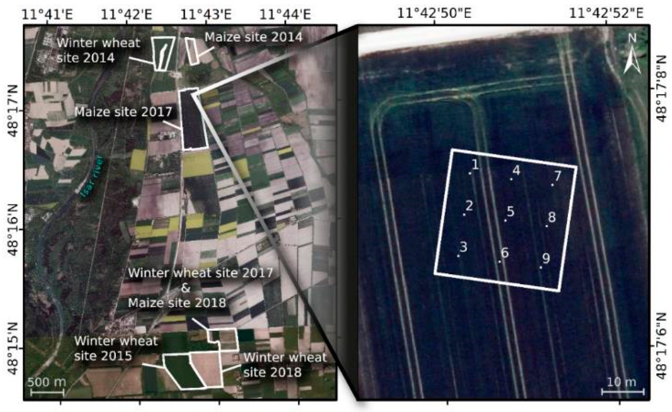
2.1. Study Site

A database of ground and remotely-sensed field data was obtained from the study area of Munich-North Isar (MNI), which is located in Bavaria, southern Germany. In the years of 2014, 2015, 2017 and 2018 the study sites (Figure 1) were visited regularly during the growing periods from March to September. Data were collected on winter wheat and silage maize fields belonging to the communal farmlands of Munich, east of the river Isar. The exact sampling sites varied from year to year due to crop rotation but all fields are located within a circle of 5 km in diameter, centred around 48°16′04″N, 11°42′45″E. Soil sampling provided no evidence of significant micro-locational (dis)advantages. An overview of all included field campaigns is given in Table 2.
Each site was confined to a 30 × 30 meters area, corresponding to an average pixel size expected from hyperspectral satellite sensors and divided into nine elementary sampling units (ESU). Data was then aggregated back to the original 30 m resolution to obtain a stable average for that date. The ESUs were revisited at each field date to guarantee solid time series.

2.2. In Situ Measurements

Canopy reflectance spectra were obtained from nadir view with an ASD FieldSpec 3 Jr. (Boulder, CO, USA [61,62]) under clear-sky conditions in the range of 350 nm to 2500 nm. Nine measurements were carried out at the same spot, averaged, splice-corrected, converted into absolute reflectance values using a white reference panel and were slightly smoothed with a Savitzky-Golay-filter [63]. At last, noisy wavelengths, that is, atmospheric water absorption bands (1360 nm–1470 nm and 1790 nm–2000 nm), were masked for any further analysis. Apart from top-of-canopy reflectances, one representative soil spectrum was recorded for each field date, serving as background information in the modelling process. In doing so, the default literature soil spectra of SAIL were temporarily replaced with in situ information and Psoil became obsolete. With nadir observations only (observation zenith angle = 0°), the sun-sensor-target-geometry is solely represented by the sun zenith angle (SZA), which was calculated from the geographical location, date and time of the observation.
Nadir RGB-photographic images were taken on winter wheat canopy scale with a Panasonic Lumix digital camera and a distance of 1.5 m above the ground. Due to the large canopy height of maize crops, no continuous series of these photographs were available for analysis of the maize site.
Average Leaf Inclination Angles (ALIA) were estimated from random samples of at least 10 leaves in vivo, using a Suunto PM-5/360 clinometer [64], which was moved along the flat leaf axis. Inclination angles of the single leaves were calculated as length-weighted averages (see Equation (1)) of those measurements and then aggregated to a mean ALIA value for the respective sampling unit.
ALIA =   1 l t o t · i = 1 n l i · θ i
with l as the length of the i-th of n leaf parts, θi as its associated inclination angle and total leaf length ltot. The conformity of that method was estimated by repeated measurements of leaf inclinations by different field workers and was found to be in the range of ±8° for the MNI campaigns. In PROSAIL, the Leaf Angular Distribution is then calculated from single ALIA values according to Campbell’s ellipsoidal distribution [65]. Leaf Area Index (LAI) was measured with a LI-COR Biosciences LAI-2200C [66] device as average of 14 measurements from the same location. The suggested sampling procedures for row crops were taken into account [67]. For early growth stages, single plants were sampled destructively and projected onto one square meter of ground area by multiplication with the factors plants per meter and seeding rows per meter.
Brown pigment (polyphenols; Cbrown), as a PROSPECT input, is rather poorly analysed in the literature. Brown leaves are usually either removed before analysis (e.g., [37,68]) or set to fixed values [69]. In some studies, it is also labelled as Content of senescent material (Cs). The variable lacks of a proper physically meaning and cannot be measured with field instruments [37]. For a start, we used Cbrown as the average “browning” of leaves between 0 (fully green leaves) and 1 (fully brown leaves) as initial guess. This is in line with Jiang et al. 2018 [70] but ignores the fact that the accumulation of brown pigments can happen without visible change of colour, which in contrast is more linked to the breakdown of leaf chlorophyll. Total LAI is reduced to green LAI by multiplication with a greenness factor 1 − Cbrown.
A Konica-Minolta SPAD-502 handheld device [71] served to measure internal SPAD-units, which were converted into leaf chlorophylla+b contents (Ccab) via an instrument-specific calibration curve. Reference data on in vitro Ccab was obtained by applying the coefficients of Lichtenthaler [72] to spectrophotometric measurements of the extinction of chlorophyll solutions. From Ccab, the carotenoids content Ccar was derived by way of a linear regression model, since Ccab and Ccar showed a stable relationship for healthy green vegetation [73]. When the linear relation breaks down for senescent stages, errors for Ccar carry only a marginal weight, because the overall biomass—as represented by the LAI—is low and has little impact on the reflectance signatures. Equivalent Water Thickness (EWT) was determined from the mass difference of sample leaves per unit leaf size before and after dehydration to constant weight (minimum 24 hours) in a laboratory oven. Leaf Mass per Area (Cm) is obtained by putting the mass of the dried leaves in relation to their one-sided surface area. The structure parameter (N) is calculated from Cm according to the inverse of Equation (2), given by Jacquemoud and Baret (1990) [37]:
LSA =   0.1 · N + 0.025 N 0.9
which (for N ≠ 0.9) yields
N =   L S A · 0.9 + 0.025 L S A 0.1
with LSA as the Leaf Specific Area, which is the inverse of Cm (note the conversion of dimensions):
LSA   [ c m 2 m g ] =   C m [ g c m 2 ] 1 ÷   1000   [ m g g ]
The variable distributions of the in situ measured parameters of wheat and maize for all field campaigns are summarized in Table 3.
The N parameter, as derived from Cm, ranges between 1.4 and 4.4 for wheat and between 1.3 and 3.6 for maize, with an average of 2.2 and 2.0, respectively.
Quantification of the phenological stages is taken from the BBCH Monograph [74], which is based on the perhaps better-known Zadoks scale [75]. No small-scale differences in plant development were observed within the 30 × 30 meter pixels. The code attribution is listed in Table 4.

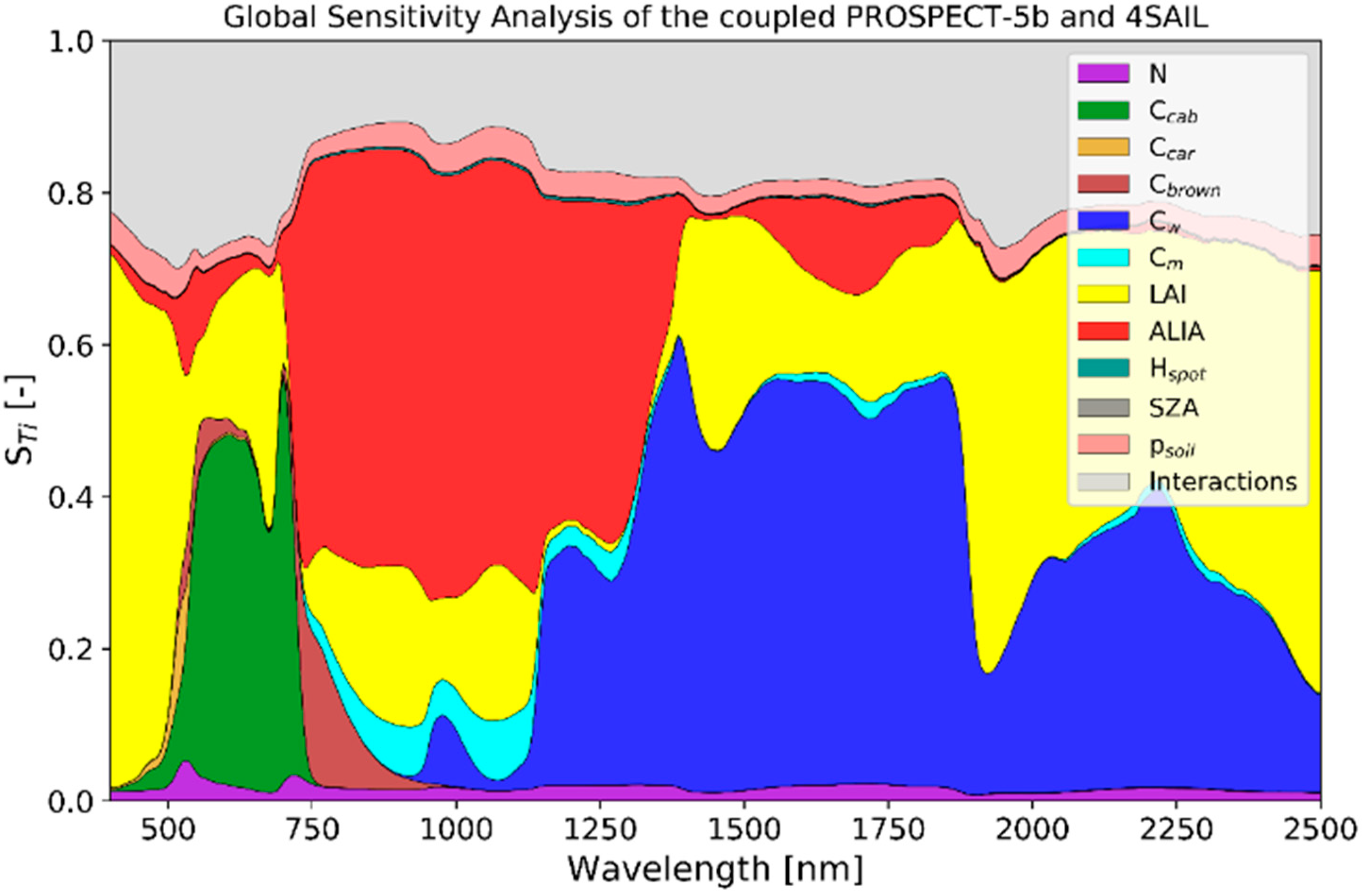
2.3. PROSAIL Environment

All data analysis was done with Python 3.6. For this reason, PROSAIL was first translated into Python code and improved in terms of computational performance by making use of C-based numerical python arrays [76] and substitution of recurring function calls by fixed local variables and look-up-tables.
For this study, we introduce the Interactive Visualization of Vegetation Reflectance Models (IVVRM) tool [77], which is an application in the open source software package EnMAP-Box 3 [78] and serves as a graphical user interface to work with data of multiple constellations of PROSPECT and SAIL. It was originally designed to offer ad hoc visual response to interactions with the model for educational purposes. Sliders can be accessed to change the value of the structural and biochemical input variables with each interaction causing an immediate re-calculation of the model output, which is displayed in a plot canvas. The tool was further extended with the possibility to overwrite the PROSAIL default background spectrum by a user-defined data vector and with an import function for any other in situ spectral signature. Those reflectances are then plotted in the same graph and—given an identical set of bands—multiple distance measures are instantaneously calculated and returned in the plot. These functions combined allow for a manual fitting between model output and in situ spectra, when model input is altered such that there is a minimal distance between the two spectra. The success of the spectral fitting can either be assessed with statistical measures like the root mean squared distance (RMSD, see Equation (5)) or visually with the degree of congruence of the curves in certain wavelength regions.
RMSD =   1 n ·   i = 1 n ( R measured ( λ i ) R simulated ( λ i ) ) 2
In Equation (5), Rmeasuredi) is the measured and Rsimulatedi) the modelled reflectance at wavelength λ for the ith spectral sensor band. n is the total number of bands analysed. The same equation works for the Root Mean Squared Error (RMSE), which was used to denote errors in the estimation of variables. By squaring the distances, information is lost about which of the terms is larger, that is, whether the model overestimates or underestimates the spectra measured in the field. In such cases, a simple mean deviation (Equation (6)) can be calculated alongside to the RMSD.
Mean   Deviation =   1 n ·   i = 1 n ( R measured ( λ i ) R simulated ( λ i ) )
The SAIL parameter skyl controls the ratio of diffuse to total solar radiation incident on the target. It is calculated in dependence of the sun zenith angle according to the approach of François et al. (2002) [79], which considers an average state of atmospheric conditions aligned to mid-latitudes:
skyl =   0.847   1.61 · sin ( 90 ° S Z A ) +   1.04 · sin 2 ( 90 ° S Z A )
The dependency between skyl and SZA is non-linear. Lowest SZA (27.8°) results in skyl = 0.24, highest SZA (70.5°) in skyl = 0.43. The mean SZA of all dates was 41.1° which corresponds to skyl = 0.23. In PROSAIL, skyl is considered uniform over the optical domain, neglecting effects of stronger Rayleigh scattering for shorter wavelengths.

2.4. Variable Fitting

In situ measured variables that serve as input parameters for PROSAIL were manually adapted to match the model output with field spectral data. The altered variables are then called optimize— or opt—in the sense that they are better suited to represent the spectral behaviour of the analysed crops in the model environment of PROSPECT and SAIL. Even though PROSPECT-D has been shown to outperform its predecessors [36], in this study we used the previous version of PROSPECT-5b. The main reason for this is that anthocyanins (Canth) were not measured in situ and deriving Canth from spectral indices retrospectively without the possibility to validate these findings would induce another error source. Three main variables were identified for optimization to achieve proper agreement between measured and modelled reflectance signatures: ALIA, EWT and Cbrown. The tuning of PROSAIL canopy geometry was necessary to cope with the large deviations that occur when comparing real and synthetic data. A global sensitivity analysis (GSA) was performed with the Fourier Amplitude Sensitivity Test (FAST) using the GSAT tool [80] in Matlab. This way, the impact on modelled plant reflectivity was assessed in the range of 400 nm to 2500 nm with a five nm sampling width for all input variables of the used PROSAIL version (see Figure 2).
ALIA was changed to obtain minimal deviations between modelled and measured spectra by using the interactive toolbox IVVRM (see Section 2.3). The success of this fitting process was monitored in the NIR spectral domain from 760 nm to 1300 nm, where ALIA shows the highest sensitivity and relative changes within SAIL. ALIAopt is thus obtained but the exact shape of the measured spectrum could only be represented when EWT was changed into EWTopt at the same time. Again, the NIR range was chosen for this task, since inversions from the SWIR domain are known for saturation tendencies whereas the 970 nm feature considers highest radiation penetration depths for stacked leaves in a canopy due to strong vegetation reflectance and transmittance [81,82,83]. Finally, Cbrown was subjected to the same calibration process. This does not have an impact on the results of EWTopt, because Cbrown,opt was determined by signature matching in the red edge (<900 nm). Manual fitting may seem unusual, given the vast majority of studies that use look-up-table inversions or numerical solutions for inversion tasks. However, the drawback of possibly iterating into a local minimum is automatically avoided, since ALIA, EWT and Cbrown have different spectral responses while all other parameters remain fixed for each date. With numerical solutions, on the other hand, slight shifts of the spectra may result in quite large deviations, whereas manual fitting yielded the advantage of a combined quantitative (error measures) and qualitative (shape) assessment of the agreement between the two spectral curves.

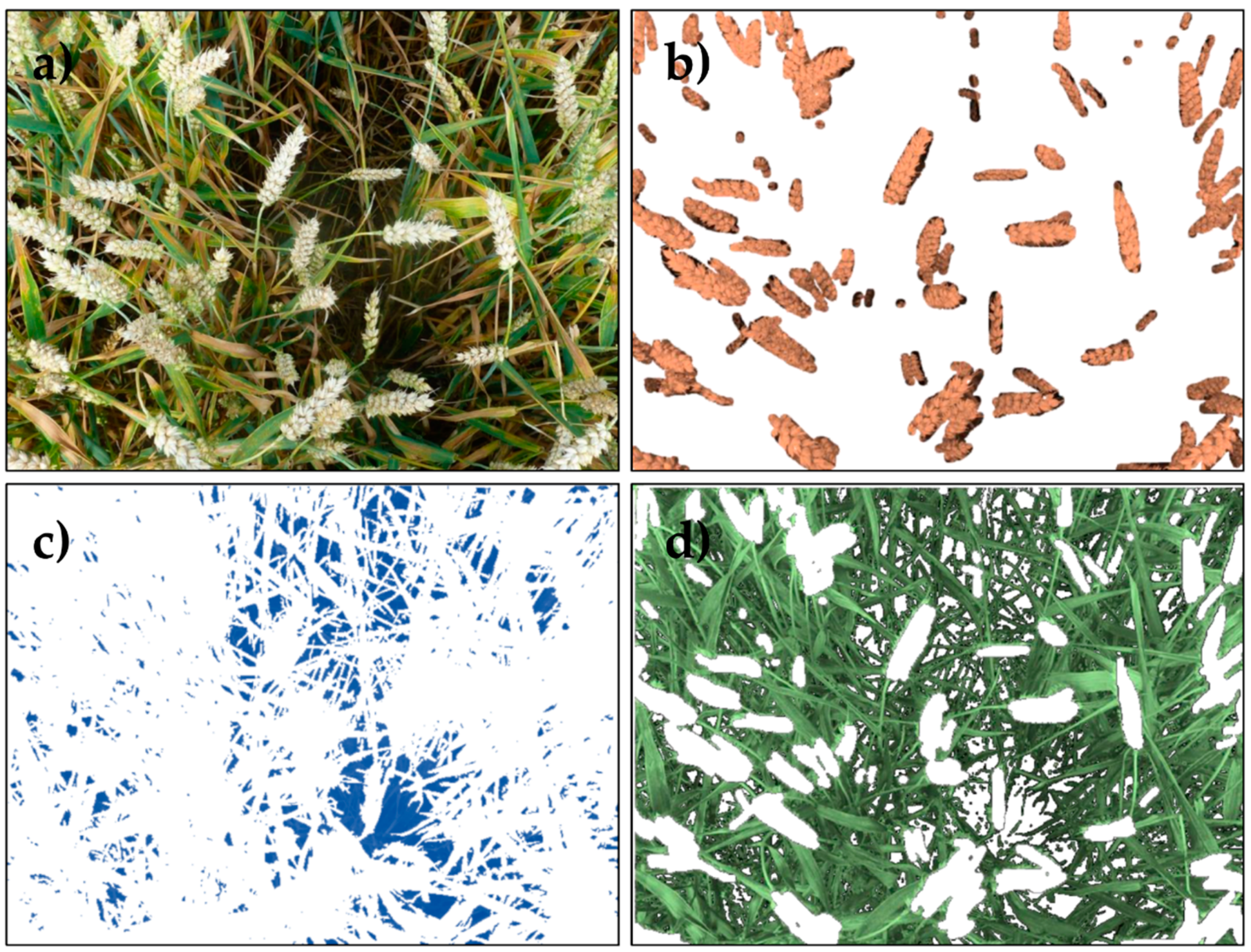
2.5. RGB Image Segmentation

Nadir RGB-images of winter wheat were processed to reveal visible fractions of the canopy (background, ears and leaves/stalks) as observed from a sensor-like position. The image processing was done with Python’s scikit-image package [84]. Images were loaded, transformed into a value range of [0, 1] and split into red, green and blue bands.
For the analysis of the background fraction, threshold values were found for each image, separating the data into dark and bright areas. Contour lines then were drawn around the darker pixel clusters and compared to the original image. At the end of an iterative process, an optimal threshold value is found and used to obtain the share of dark pixels in the image. These include not only soil pixels but also other parts of the canopy that show marginal reflectance in the visible spectrum and thus do not contribute to the canopy signature (see Figure 3c).
Determining the fraction of visible area of ears requires a preceding step, in which the ears of the winter wheat canopy are manually masked using standard CAD software. Their share was again calculated with the help of scikit-image (see Figure 3b). All pixels that are classified neither as dark background nor as ears are considered leaves and stalks (Figure 3d). They usually make up the greater share of the picture. It should be noted though that these fractions could not be directly considered as linear contributors to the total spectral range of the sensor, because the RGB camera only captures wavelengths from 400 nm–750 nm, while vegetation transmissivity especially in the NIR domain can be higher compared to the VIS part. The share of vegetation pixels from nadir view is often referred to as fractional cover (fcover) and the background fraction fbackground = 1 − fcover, as the gap fraction.

3. Results

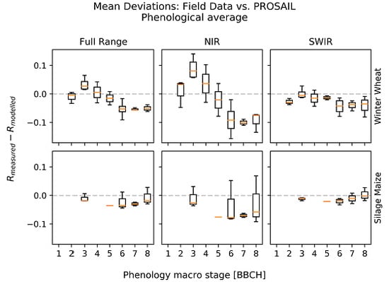
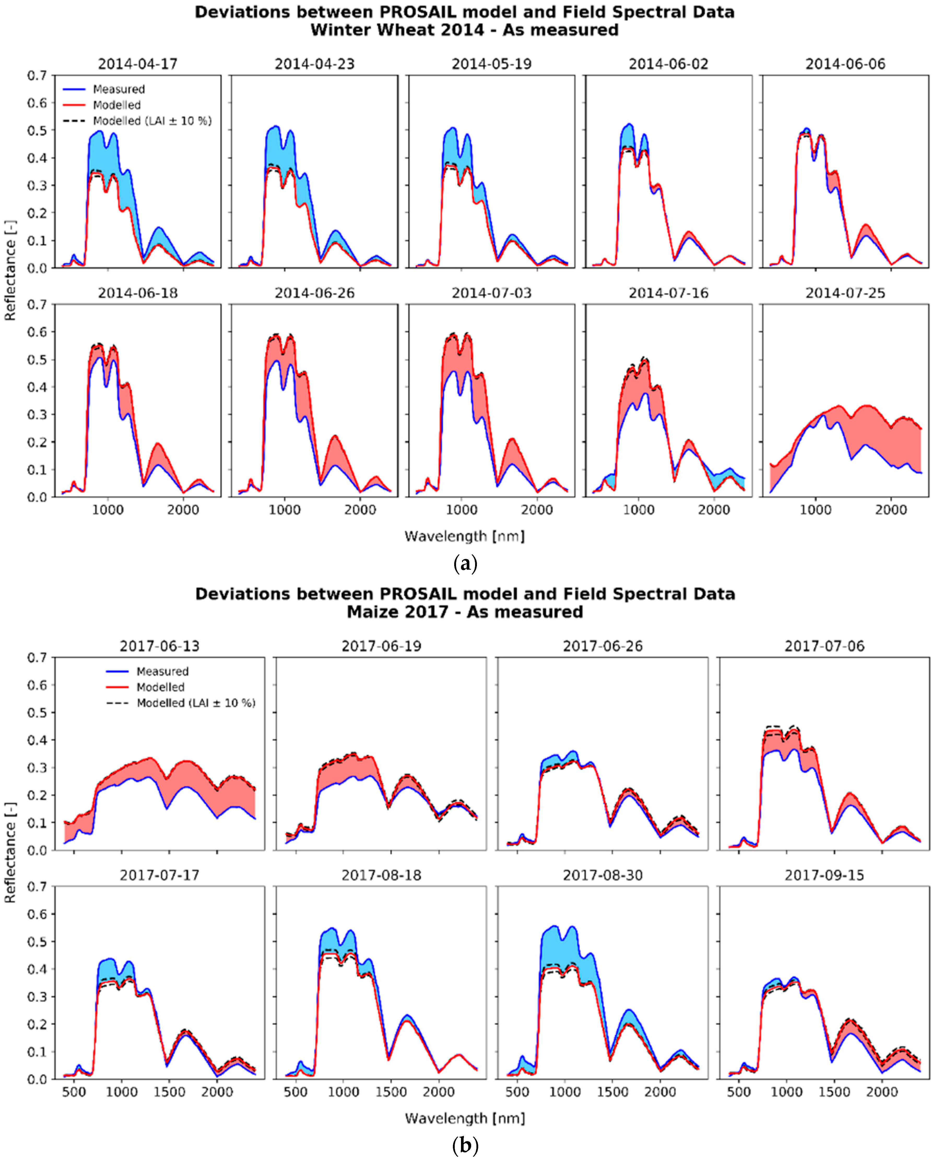
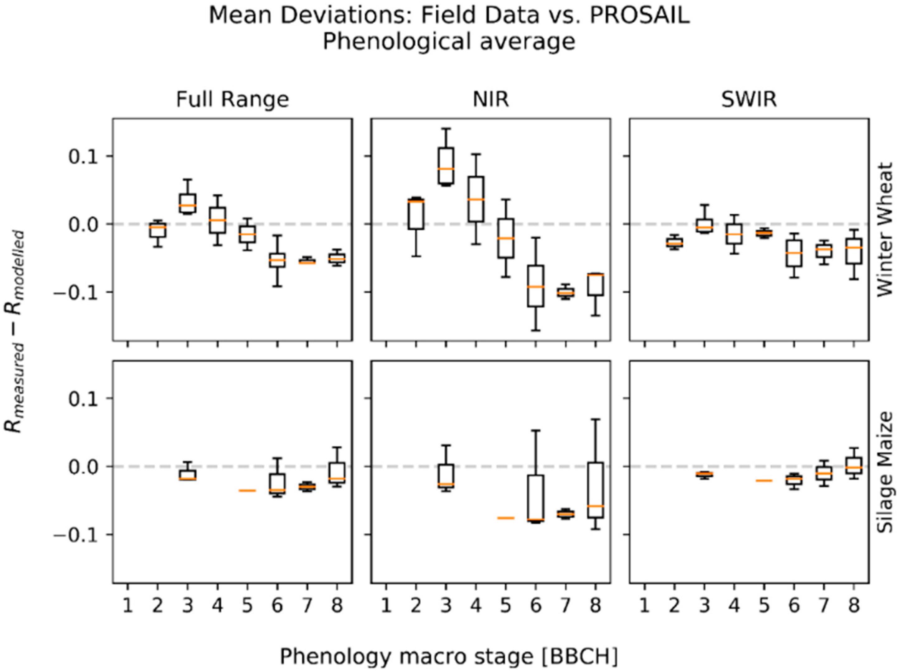
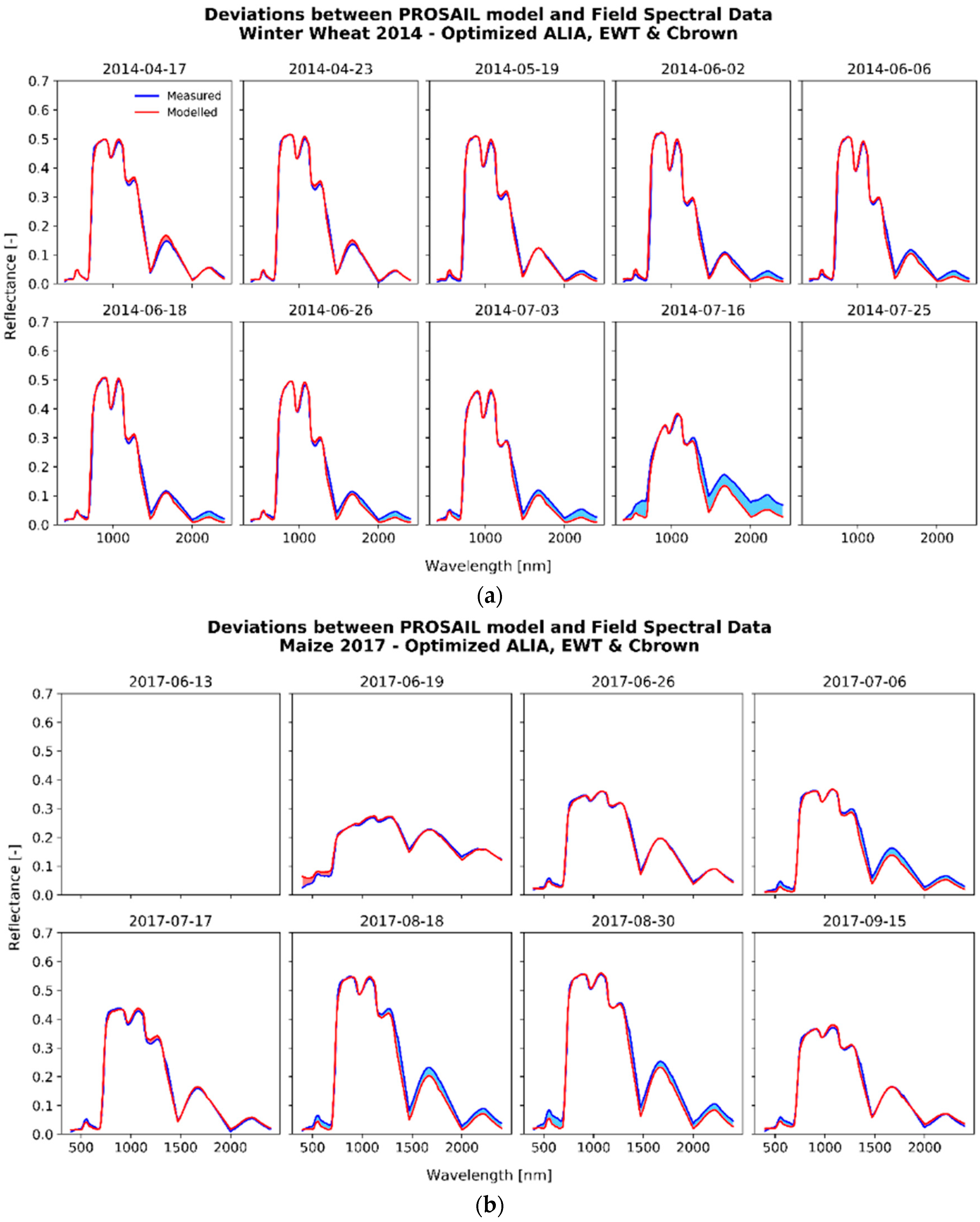
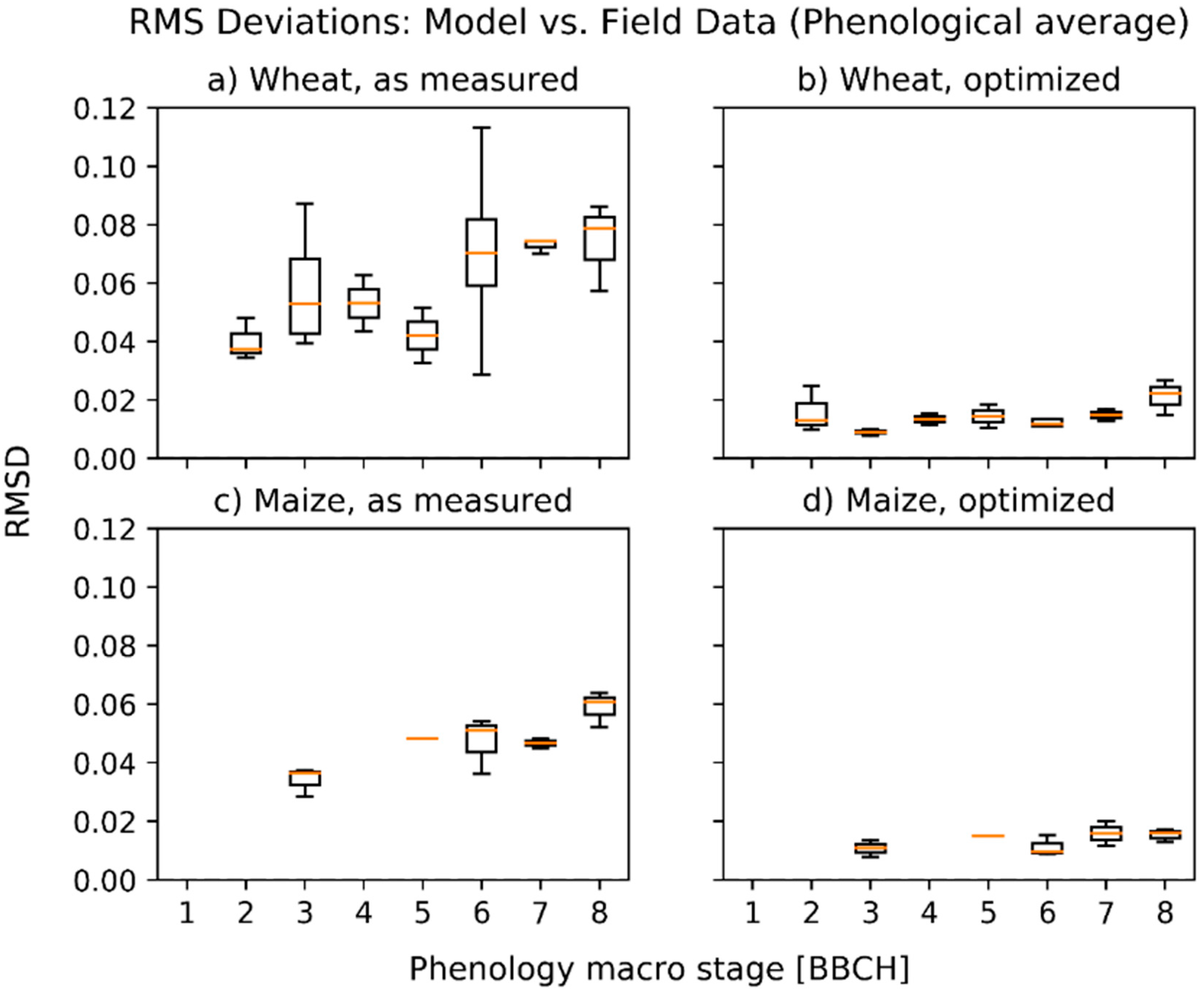
3.1. Deviations between Model and Measurement

In situ measured variables served as input for the coupled PROSPECT-5b and 4SAIL. The spectral output of the model is contrasted with the spectral signatures recorded at the exact same spots. The results are shown in Figure 4 for winter wheat (2014) and silage maize (2017). Results of the other seasons can be found in the Supplement (wheat: Figure S1; maize: Figure S2).
In 2014, the winter wheat field campaign started in mid-April, when green biomass had already developed. In the first four field dates spanning one month, measured NIR reflectances increased, before revealing a decreasing tendency from June on. The SWIR range in contrast drops continuously until beginning senescence. PROSAIL output on the other hand did not capture this pattern. Modelled spectra in the NIR rise from date to date, reaching a maximum in early July (3 July 2014). In the SWIR, modelled spectra behave exactly opposite to the measured signal with a peak at 1750 nm successively climbing from 0.08 at the beginning of the series to 0.22 at fruit development stage. In this regard, the underestimation of spectral signatures by PROSAIL gradually gave way to an overestimation.
Looking at the data of the other seasons (see Figure S1), this pattern proves to be recurring. In 2015 and 2017, spectral and in situ data was recorded already at early growth stages of leaf development and formation of side shoots. At that time, modelled reflectances were constantly higher than those measured on site. In summary, two tipping points are observed: (1) from overestimation to underestimation (end of March; shoot development) and (2) from underestimation to overestimation (beginning of June; inflorescence emergence). Figure 5 illustrates this pattern by plotting mean deviations as PROSAIL output subtracted from field spectra. Aggregation into phenological stages allows a comparison independent of the growing conditions of each year. Patterns are similar for deviations in the NIR and SWIR, only the absolute values in the NIR were generally higher, thus so are the deviations.
Maize reflectances for 2017 were overestimated by the model for early growth stages, when fractional cover was low, and LAI ranged below 0.7. These stages were followed by a period of model-underestimation in the NIR (with exception of the aberration at the 6 July 2017 date) and signal increase in the SWIR that is not present in the model output. In the other seasons, there was no general trend in the deviation between model and measurement (see Figure S2). For 2014, SWIR reflectances are captured well by the model but the NIR plateau was overestimated throughout the season. In 2018, a massive model-underestimation was recognized for 21 June 2018, which seems to be a single event or measurement outlier. The seasonality of deviations is analysed by calculating a simple mean of Rmeasured minus Rmodelled (see Figure 5). This approach may cancel out a non-uniform behaviour of different bands of the same spectrum, so the results are separately shown for NIR and SWIR where deviations show a generally high coherence. Said deviations are less distinct for maize than for winter wheat. For this crop type, a predominant model underestimation is observed in all phenological states instead.

3.2. Optimized Parameter Sets

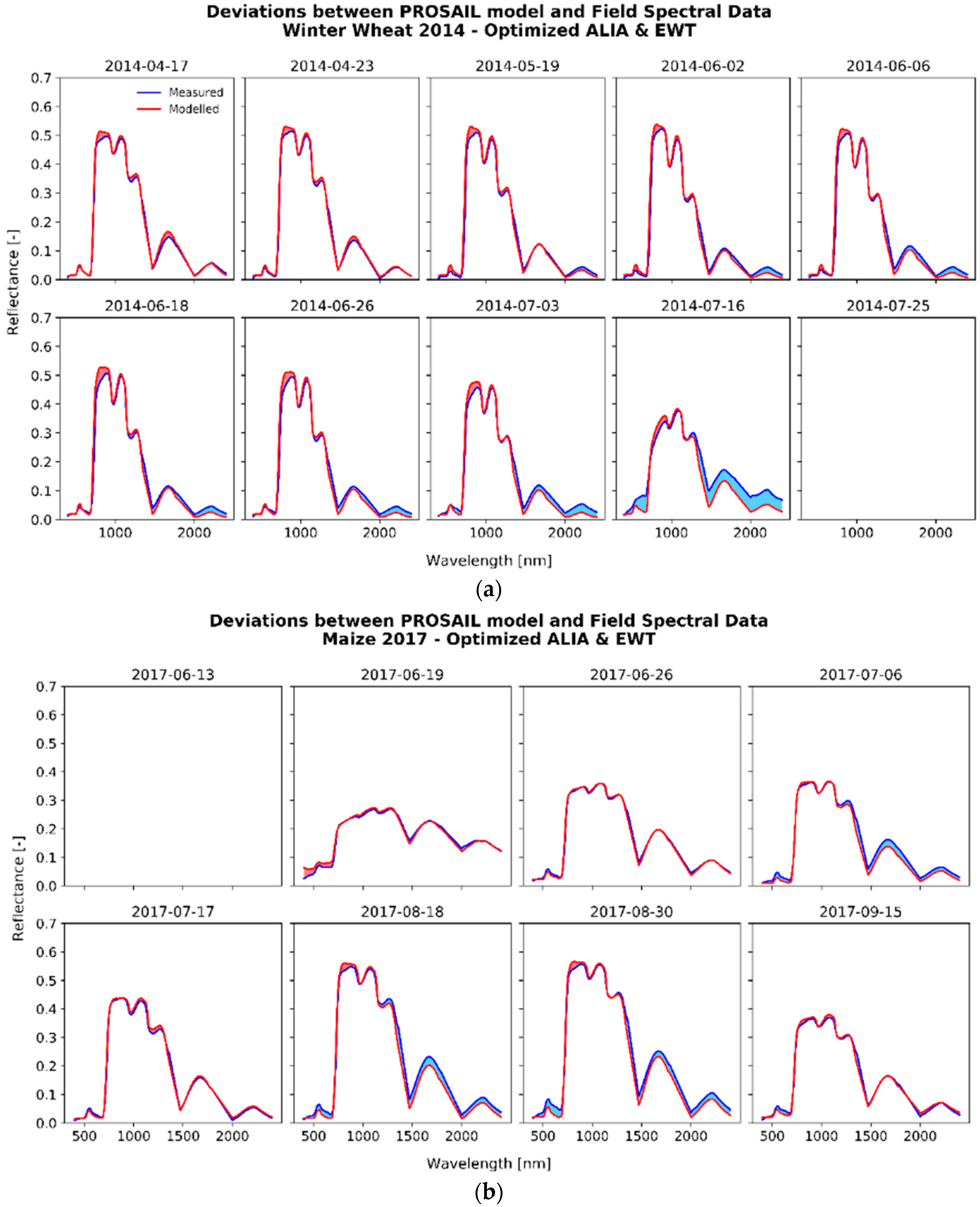
3.2.1. The Fitting Process

The fitting of ALIA and EWT led to a better agreement for example, for the 2014 winter wheat (Figure 6a) and the 2017 silage maize (Figure 6b) dataset – illustrations of all seasons are found in the Supplement (wheat: Figure S3; maize: Figure S4). But even after the first manual optimization, both crops show an overestimation from the red edge to the NIR shoulder. More precisely, PROSAIL models a plateau-like shape in this region with a distinct convex edge, which is not present in the field spectra. A beneficial solution for this occurrence is the fitting of Cbrown into Cbrown,opt. This second step is demonstrated for the same example years for wheat (2014, Figure 7a) and maize (2017, Figure 7b) The results for the final optimization of the other years are found in the Supplement (wheat: Figure S5; maize: Figure S6).
Even though there were individual differences in the development of deviations between measured and modelled spectra for the four growing seasons, there is a greater pattern recognizable. To make these independent of the Julian days, those deviations were averaged for all macro stages according to the BBCH-scale (Figure 8) as RMSD values. Deviations for winter wheat are largest for the original data with elevated errors in the stages of stem elongation and booting as well as for fruit development and ripening (Figure 8a). After adapting to the measured spectra, deviations stay within a narrow boundary below 0.02 reflectance with smaller values for stages of intensive production of fresh green biomass and greater ones at crop maturity (Figure 8b).
In contrast to winter wheat, deviations between modelled and measured spectra of silage maize showed no seasonal fluctuation neither before nor after ALIA, EWT and Cbrown were altered (Figure 8c,d). RMSDs only increase with ongoing phenological development and are on average 18% lower, indicating a better predictability for maize canopies than for winter wheat. Please note that macro stages 2 and 4 do not exist in the BBCH phenological categorization for maize.

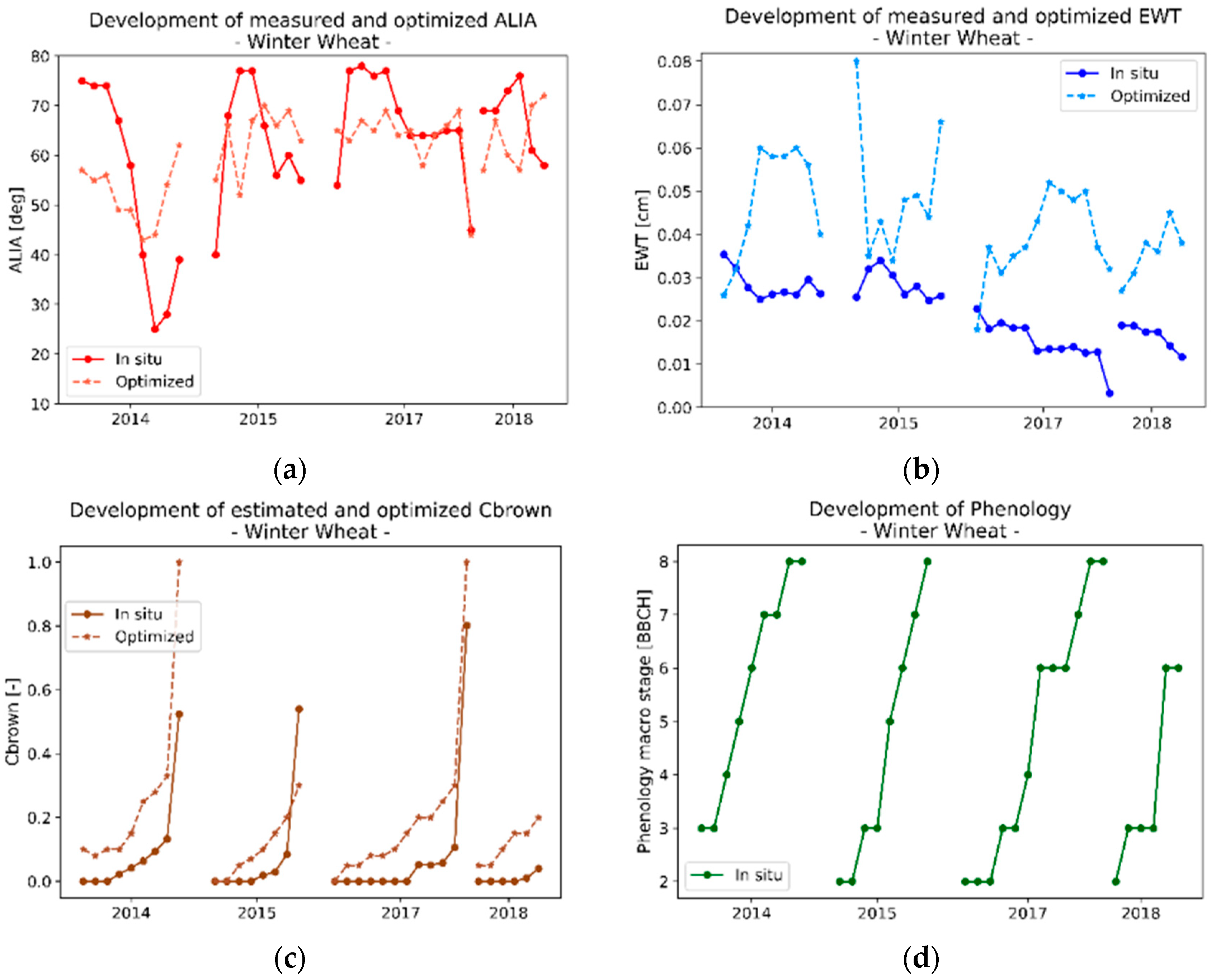
3.2.2. Analysis of the Optimized Variables for Winter Wheat

To analyse the correspondence between measured and optimized variables, their seasonal progress is plotted in Figure 9 and their correlations are listed in Table 5. A full comparison between ALIA, EWT and Cbrown as observed in situ versus the results of the two-step manual optimization process is listed in the Supplement for all field dates of the four seasons of winter wheat field campaigns (see Table S1).
The development of ALIA is quite stable in all seasons of wheat. After high inclinations at the beginning of the growing period, leaves tend to bend down and finally surpass the 0° horizontal line to point towards the soil, which again results in increasing angles for senescent stages. These tendencies are only partly illustrated in Figure 9a, because field dates with low LAI were not optimized and are omitted in the graph. Still, winter wheat reveals notable deviations between these findings and the calibrated ALIA values. RMSEs range from 8° to 18°, which corresponds to relative RMSEs of 0.19 and 0.34. Inter-seasonal variation was 29%. A negative slope for the 2018 regression (R2 = 0.77, slope = −0.85) and the low R2 of 0.18 for the complete time series affirm the impression that ALIAopt is independent of the original ALIA.
For EWT, even stronger seasonal patterns are visible. Young wheat leaves hold highest water contents but then continuously desiccate with only rare disturbances, for example, in the early growth cycle of 2015, when the canopy first had to recover from a particularly dry spring. When approaching late senescence, leaf water drops <0.01 cm. After fitting the spectral signatures in the 970 nm and 1060 nm region and comparing EWT with the fitted EWTopt, relative errors between the two variables range between 0.87 and 1.8 and are 1.18 for the complete time series of four years. This means that the distance of the optimized EWT to its original field representation on average ranges beyond 100%. EWTopt follows a different seasonal pattern connected to the green biomass. In fact, correlation between EWTopt and LAI range between R2 = 0.27 (2014) and R2 = 0.6 (2017), confirming the bias present in the data.
In situ estimations of Cbrown were 0.0 during the vegetative stages of winter wheat. Canopies showed no senescent spots on leaves until beginning of ripening. Once senescence was initiated also in the top layer of the canopy at the beginning of July, Cbrown skyrocketed within a few days’ time. With these in situ measured values, however, no sufficient fitting was possible in the red edge region. A better match with modelled spectra was obtained when Cbrown,opt was continuously increased throughout the season. Deviations are in a constant range from 0.1 to 0.2. Similar to EWT, the relative distances to the increased optimized variable set reach disproportional magnitudes due to absolute values below 0.1 (see Figure 9c). It is worth noting, though, that Cbrown is correlated with Cbrown,opt. The slope of the regression for all four seasons is 0.25 and the intercept is 0.13, which can be considered as a significant bias (p = 0.017) that occurs right from the beginning of each season and could be accounted for with a linear model.

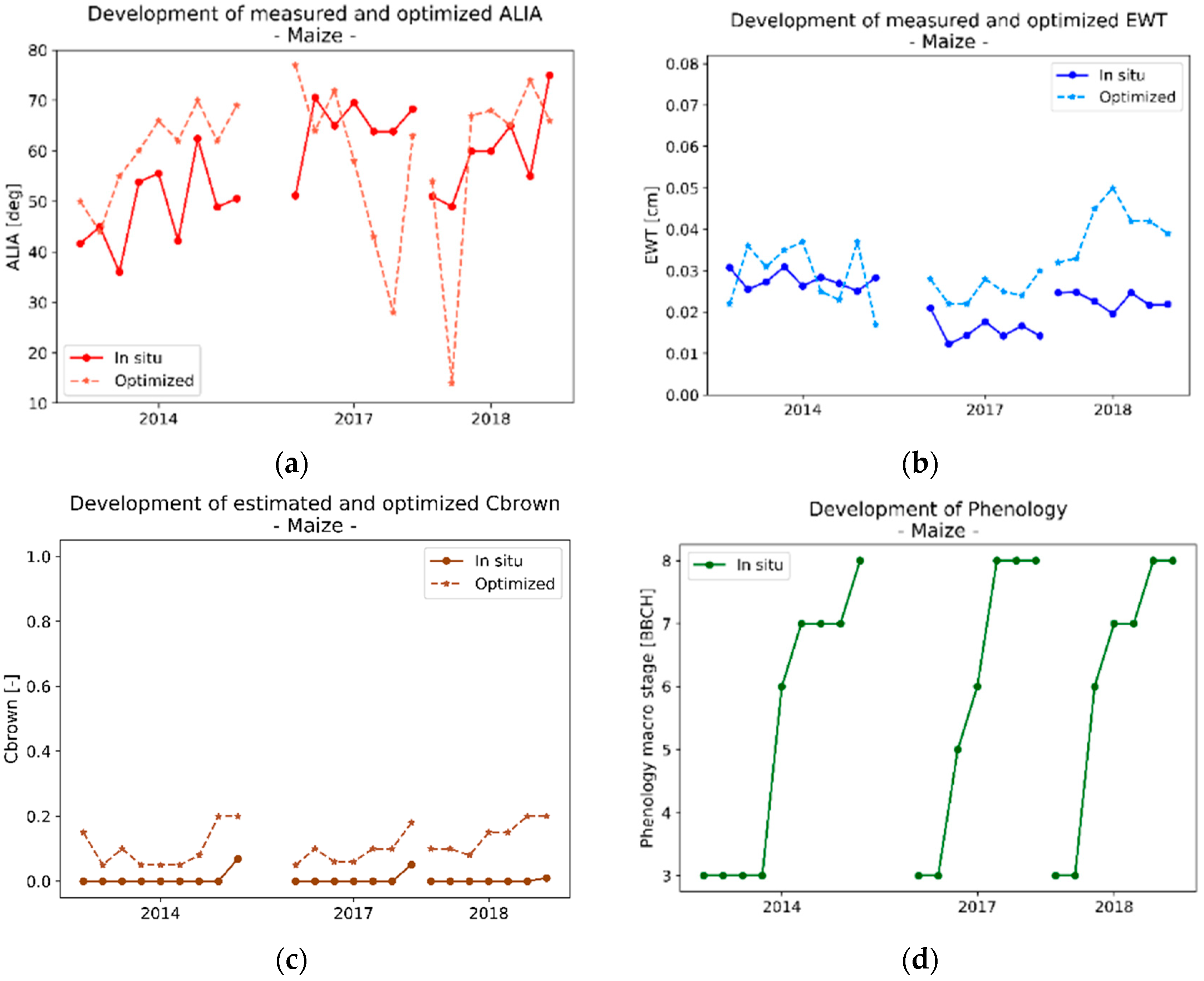
3.2.3. Analysis of the Optimized Variables for Silage Maize

In the same manner as it was done for winter wheat, the illustration of the development of the measured and adapted maize variables is shown in Figure 10 and the secondary statistics are summarized in Table 6. In situ records in full are listed in Table S2.
According to the in situ measured variables, ALIA of maize shows an erratic seasonal trend towards increased inclinations at ripening stages. Intact leaf tips of younger maize plants pitch over but get more and more rigid in their reproductive states. Shortly before vegetation dieback, leaves sag down in parallel direction to the stalks resulting in high inclination angles. This pattern is observable for all three seasons and partially reflected by ALIAopt. Large deviations in the modelled ALIAopt occur as singular events at the end of 2017 and the beginning of 2018.
Inter-seasonal variability of EWT for maize was higher than the inner-seasonal changes. In contrast to winter wheat, water content in maize leaves was stable in all seasons. An intense loss of plant water happened only at the very end of the maturity stage beyond the time series used for fitting the spectra (not shown). The generally lower EWT in the 2017 data suggests a reduced water availability in that year for the respective soil condition of that field despite good meteorological conditions. EWTopt shows significant concordance with in situ values for 2018 but the large relative errors indicate the overall weak predictive power of a PROSAIL simulation even if based on measured ground data. A bias towards biomass is similar to the findings for winter wheat: R2 with LAI range between 0.33 in 2014 and 0.67 in 2018.
Cbrown was 0.0 for all phenological stages of maize until cob ripeness. At senescence, water content dropped, and little brown spots became visible. Unfortunately, higher values of Cbrown had to be clipped, because they coincide with low green LAI and thus cannot be reasonably optimized. Despite this fact, Cbrown,opt—as parameterized in PROSPECT—needs to be increased right away at stages of leaf development and booting to account for non-visible accumulation of brown pigments within the leaf. This is confirmed by the volatile trend of Cbrown,opt particularly in the 2014 season which could not be explained by brown leaf spots alone.
When comparing the two different crops, deviations from the in situ measured leaf inclinations were found to be 20% lower for winter wheat when compared to silage maize. A main reason for that can be found in the two striking outliers of 2017 and the one in 2018. When they are excluded from the analysis, RMSEALIA for maize drops by 10% to 14.5°. RMSEEWT was twice as high for wheat than for maize.

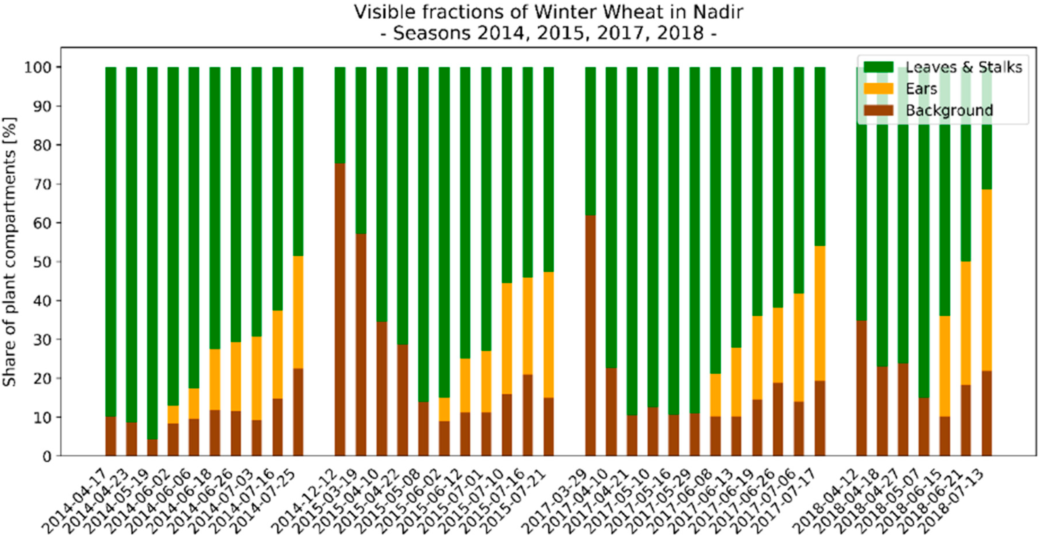
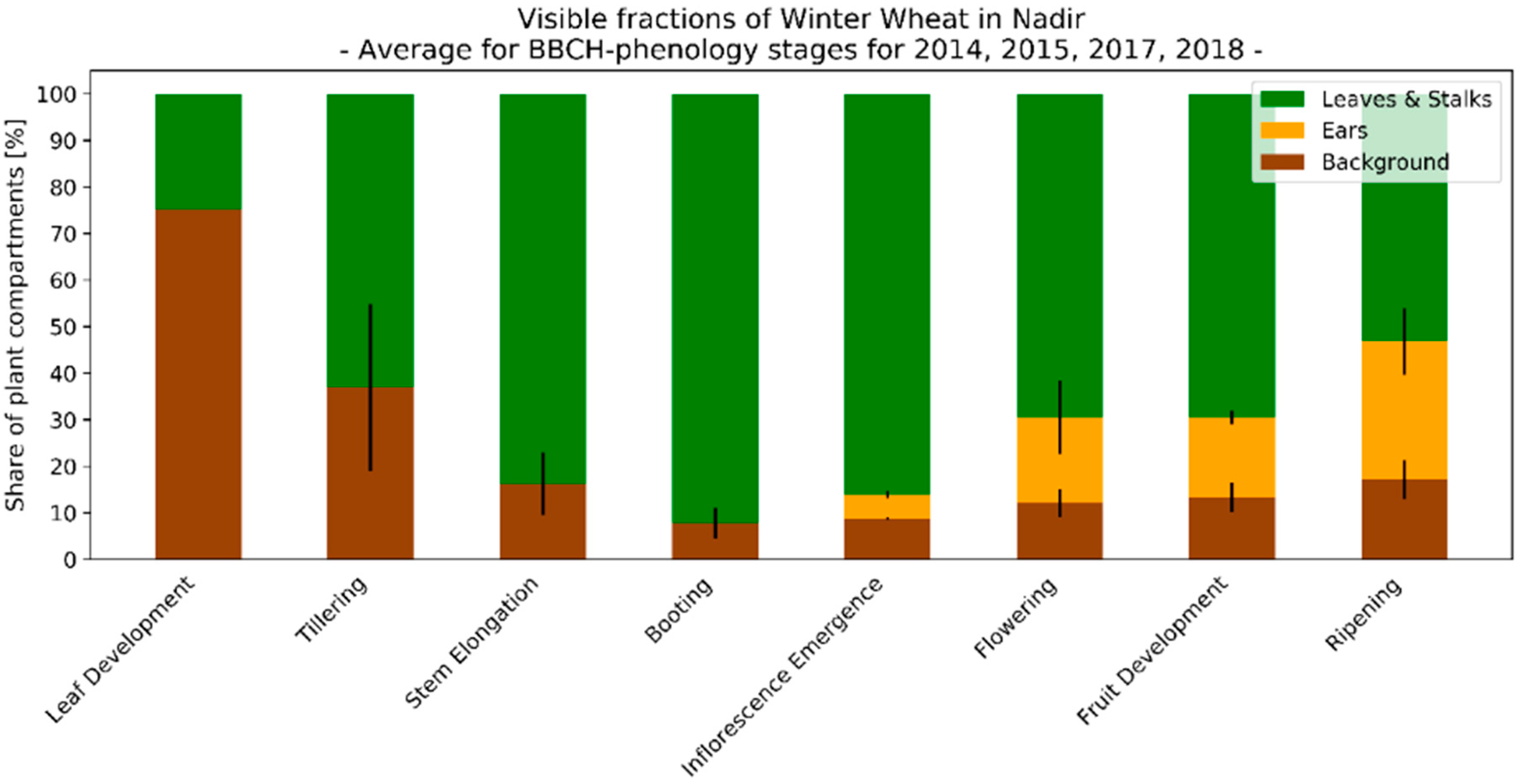
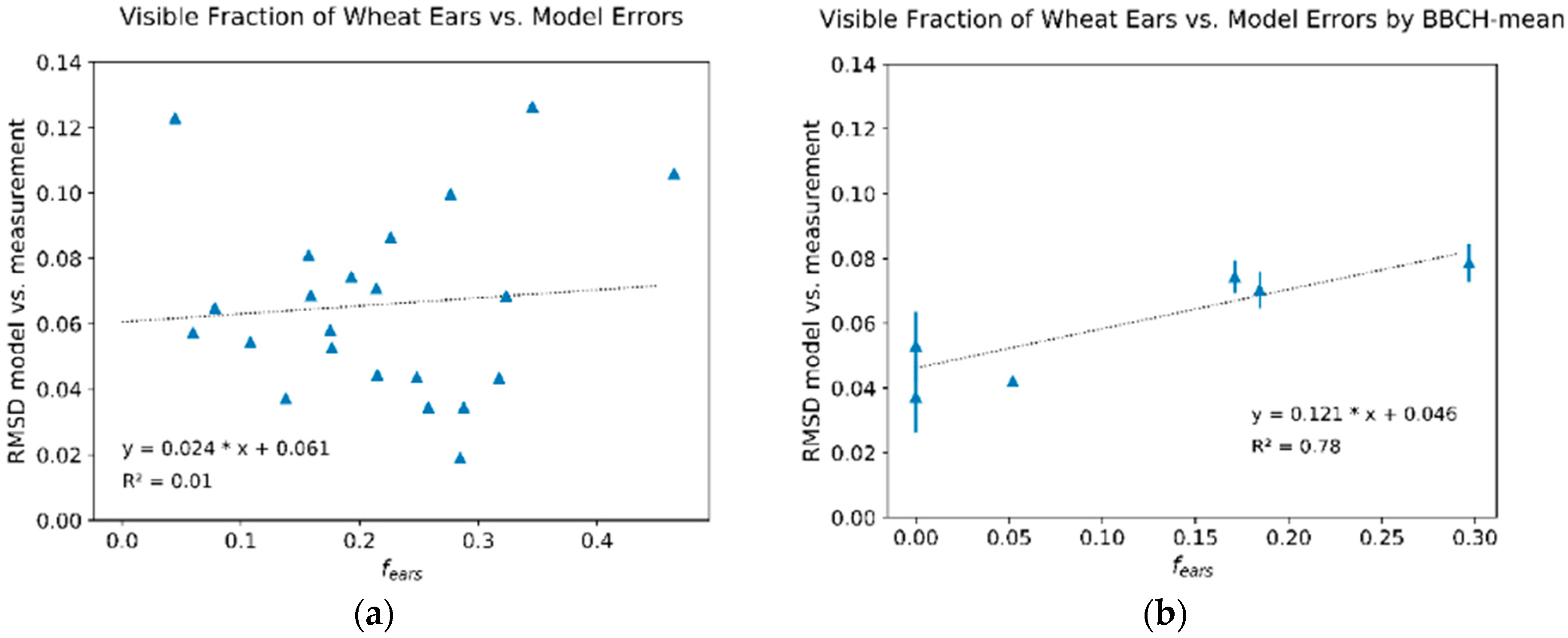
3.3. Seasonal Development of Winter Wheat Canopy Fractions in Sensor View

The mean distribution of plant fractions of the winter wheat canopies—as seen from nadir view—is shown in Figure 11. Early observations in March and of pre-winter sprouting (only covered in 2014/15) reveal a high share of background pixels. Wheat plants are small and aligned in rows at that time. After some weeks, the vegetation forms a closed canopy of leaves with only little gaps in between. The fraction of dark background fbackground then remains at a constant level of 10–20%, even when ears begin to grow. Together they extend their visible fraction up to 50% in the years of 2014, 2015 and 2017 and even 70% in the season of 2018.
The meteorological and micro-ecological conditions vary between the four seasons, which limits the comparability even for the same days of the year. Similarly to the statistical analysis of the optimized sets of variables described in Section 2.4 visible fractions of plant compartments were aggregated in their phenological macro stages to derive a representative seasonal pattern (see Figure 12). A strengthening of the trends recognized in Figure 11 can be observed. Lowest values for fbackground are found in the stage of booting, when the green canopy is dense and covers most of the underlying soil. When the wheat ears are established, their visible influence grows mainly to the expense of leaves and stalks, whereas fbackground increases only slightly. The agreement between the estimations of fbackground was highest for low values, for example, an error of 0.3% at stage of emerging inflorescence and 3.4% at booting stage and lowest for the tillering stage with an error of 18%. Errors of the visible fraction of fruit ears were lowest at emergence of the flowers (σ = 0.8%) and fruit development (σ = 1.5%) and highest for flowering (σ = 7.9%) and ripening stages (σ = 7.2%).
Combining these results with the model deviations, the relationship between RMSD and the fraction of visible ears is analysed. As shown in Figure 13, the R2 of that comparison is a mere 0.01 with a dispersed scatter plot for all data points in which wheat ears were visible in the RGB photography (Figure 13a). After aggregating the data into phenological stages, their representative values form a linear model with R2 = 0.78 (Figure 13b). A correlation between the fraction of visible soil and the RMSD by contrast could not be found. R2 for was 0.02 for all data and 0.1 after aggregation.

4. Discussion

The performance of the parameter retrieval of canopy reflectance models is usually evaluated by means of descriptive statistics, comparing measured and estimated variables and assuming that low errors indicate high accuracies [85]. This requires that model parameters and in situ variables are representing the same natural property. Our study demonstrates that this prerequisite does not apply to every case when working with PROSAIL. Model results were significantly different to measured spectra, even when in situ measured variables define the input.
Nevertheless, even reasonable measurement errors of for example, LAI could not explain the observed deviations. Remaining errors are expected to be intrinsic uncertainties of the model design linked with the degree of abstraction. RMSD between spectral field observations of the winter wheat study sites and their model representations reveal that PROSAIL describes canopy properties better for early growth stages. Consequently, they are better suited for retrieving canopy variables than later stages. Within the non-reproductive stages (BBCH 1–5) there is an additional local RMSD minimum observed when vegetation initiates the heading of the ears (BBCH 5). This phenomenon is not seen in the maize dataset but the tendency towards increased errors with passing phenological stages here comes with an overall better agreement between model results and spectral measurements.
In PROSAIL, the ALIA plays an important role among structural model parameters with high total scores in the global sensitivity analysis, particularly in the NIR. The biomass density of the canopy is quantified via LAI and manifests in the spectrum through stronger reflectances in the NIR and stronger absorbance in the SWIR. For increased LAI, a saturation in the SWIR by water absorption in optically thick canopies was mentioned by, for example, Datt et al. [86]. In PROSAIL, high reflectance levels of the NIR plateau can only be simulated when assuming low ALIAs. Take note that SAIL is not a geometrical but a radiative transfer model. The incorporation of leaf inclination into the preceding Suits model [87] allowed accounting for the scattering processes that happen within the canopy. Leaf angle densities are calculated according to Campbell [65] representing frequencies of leaf inclinations as discrete classes. For each class, the volume scattering is calculated resulting in the Suits system coefficients, which denote contributions for each inclination class to the basic radiation transfer processes of extinction, attenuation and backscattering from the canopy. The LAI later serves as a scaling factor of these processes. This means that in PROSAIL the ALIA is used to estimate probabilities for radiation to be absorbed, attenuated or reflected. In reality, wheat fields are densely seeded, and the complex canopy structure appears closed from tillering stage (BBCH 3) onwards, even though ALIA at that time shows values above 70°. Any kind of minimization between model results and measured spectra therefore suggests a lower ALIA to capture high reflectances in the NIR caused by multiple scattering in thick canopies, especially in stages of intensive biomass production and growth [88,89]. After this period of stretching wheat leaves, the ALIA decreases and is soon overestimated by the model. This could be an indication that ALIAopt aims to reproduce vertical canopy structures, that is, stalks or fruit ears with high inclinations that make up 18% (flowering) to 30% (ripening) of the nadir view. In this regard, winter wheat seems to conflict with the basic turbid medium assumptions of scattering objects of infinitesimal size, disallowing shadowing within the canopy. Also in 4SAIL, the finiteness of leaves is only accounted for by the hot spot effect [90], while consideration of precise geometrical structures is still confined to 3D ray tracing models. Nevertheless, it was conversely expected that 4SAIL presumptions would rather fail for maize. It consists of much larger leaves aligned in a more heterogeneous canopy than wheat fields. Single plants grow larger and form a distinct row structure. It seems that overlapping leaves in the wheat field become stacks of green biomass within the canopy, even for erected leaves. Maize plants stand more isolated and allow radiation to penetrate deeper into the stand. The consideration of using 4SAIL to retrieve vegetation parameters independently of the vegetation type accordingly does not fully hold true.
The estimation of LAI from hyperspectral data has been sufficiently described by other authors, unlike the retrieval of ALIA, which is often treated as a free parameter without final assessment. Few studies took up this issue, like Casa et al. [91] who could not achieve adequate estimates of ALIA for maize data from PROSAIL optimizations but found lower deviations when leaf inclinations were obtained from measured gap fraction data. The visible fraction of soil as an alternative to the gap fraction in this study did not correlate with optimized ALIA and thus turned out to be inefficient for an improvement of PROSAIL inversions. Botha et al. [92] retrieved canopy structure variables from PROSAIL as a side product to leaf chlorophyll content estimation of wheat canopies, struggling with low correlations between measured and estimated ALIA. They further experienced an overestimation of LAI except for the first growth stage. This supports our finding that wheat reflectances in the NIR are higher than modelled for given LAI in situ data in the essential growing period.
In the first PROSAIL review by Jacquemoud et al. [34], it was stated that spectral responses of LAI and ALIA were closely correlated with each other, making an independent inversion of those parameters problematic. Other studies have tried to overcome this deficit by providing statistical information as a priori boundaries [55], classifying ALIA within a narrow parameter range [93], transforming two-band-indices [94,95] or incorporating the information of pixels in spatial vicinity to obtain an object-based result [96]. Our proposed manual calibration of ALIA could potentially serve as another separation approach when the LAI has been reliably estimated. In all cases, a successful decoupling of canopy structure parameters is aided by integrating multi-angular observations in the inversion process [93,97] for example, from CHRIS/PROBA or future EnMAP.
In situ measured EWT did not agree with the values obtained from the optimization process. One reason is the complex canopy structure linked to the type and amount of biomass observed from the sensor. In the spectral signal, there is no differentiation between phyto-elements of the crop, whereas the model considers EWT as a pure leaf parameter. Figure 14 shows that wheat stalks contain more water than the leaves per unit fresh mass from June onwards (BBCH 4). Thick maize stalks contained more water than the leaves at all times in the growth cycle. Errors between EWT and EWTopt were conversely higher for wheat than for maize, indicating that EWTopt carries even more residual information of canopy features, which is in line with Clevers et al. (2010) [98]. The interleaving of foliage may lead to an additional vertical stacking of biomass and exaggeration of biophysical and biochemical features in the model. Inversion of PROSPECT alone was shown to produce adequate results for estimation of EWT [99,100,101], whereas the proper retrieval from complex canopy spectra remains a difficult task [102,103]. Another solution to this problem could be crop- and phenology-specific calibration curves if further research confirms the relationship between EWT and EWTopt found for wheat in the four seasons presented.
The need for a proper parameterization of Cbrown becomes apparent when observing the residual deviations in the red edge region and the absence of a distinct shoulder in the field spectra (Figure 6). The same spectral shape is found in other publications that analyse dense crops like winter wheat [104] or grassland [51]. Solid assumptions about the biochemical influence of brown leaf pigments are necessary to improve the quality of the retrieval of other plant pigments as well as of LAI and ALIA, which are all sensitive in the far red and NIR. The variable Cbrown generally lacks a solid scientific study basis. There is no evidence of a successful inversion of Cbrown in the literature and for forward mode simulations it was often used as a calibration parameter for the spectral region from 500 nm to 1000 nm. The authors of PROSPECT state that the disturbance around the NIR plateau occurs at senescence and for dry leaves [35]. Results of our study show that brown pigments play an important role even for vital green canopies, particularly for maize. Further research should be directed towards proper estimation and interpretation of Cbrown, identifying valid ranges for different crop types and the relation of Cbrown with crop phenology to assist the estimation process. Treating Cbrown as visible leaf browning proved to be insufficient.
Further improvement of retrieval accuracy could of course be achieved by the use of newer versions and more sophisticated modelling approaches. Anthocyanins (Canth) play an important role in the photo-protection of plants [105] and their incorporation into PROSPECT-D was shown to particularly improve the retrieval of carotenoids [36]. But even if Canth had been considered for this study, impact on the calibration of Cbrown is expected to be low, considering that the latter was adjusted through spectral matching in the red-edge region (750–900 nm) in which Ccar is not sensitive (see Figure 2). The same holds true for the deviations occurring in the RED region, which indicate a potential issue in the retrieval of Ccab at crop ripening. Running such fitting procedures with different versions of PROSPECT could further identify the role of parameterization of the absorption coefficients and the refractive indices used in each model. Implementing the Leaf Inclination Distribution Function (LIDF) directly could pose a superior alternative to deriving it from ALIA with the Campbell approach, as it allows a more comprehensive description of the canopy geometry. For instance, an ALIA of 45° would result in one specific LIDF when using the ellipsoidal model but could be described by several different distributions when using for example, Verhoef’s algorithm with the parameters LIDFa and LIDFb (please refer to the review of Wang et al. 2007 for an overview of that topic [106]). Splitting the information into two parameters increases the probability to encounter ill-posed solutions but could also potentially improve the retrieval process, especially in the case of multi-angular observations. Another limitation of this study concerns the choice of the parameter set for optimization. The restriction to ALIA, EWT and Cbrown leads to an affiliation with the errors of other parameters if their sensitive spectral ranges overlap. Apart from LAI, this could also be the case for Cm, which—despite a good retrievability from PROSPECT model inversions (e.g., [107,108])—is expected to suffer from similar scaling problems like the EWT [109]. On the other hand, it remains problematic that more simultaneously adjusted parameters also result in a more severe ill-posedness. An increase in Cm leads to a decrease of the reflectance in the NIR, just like an increased ALIA does. Consequently, ALIAopt, as the result of a calibration process, will also carry a residual signal about the uncertainties of other, less sensitive parameters like Cm and the derived leaf structure parameter N.
Uncertainties in the quantification of in situ variables vary with experience of the field workers, chosen sampling layout, technical equipment and methodology. Matching model output with real spectral observations would assume that the illumination is optimally represented in PROSAIL. The ratio of diffuse to direct radiation, for instance, is controlled by the skyl parameter, which was applied as a flat spectrum instead of a wavelength-dependent data vector. A full description of lighting conditions upon the canopy would have to incorporate atmospheric modelling, taking into account the aerosol optical depth, precipitable water and O3 content [110]. For the manual fitting process, it is assumed that LAI has been correctly measured. In reality, the method of inverting the gap fraction from LAI2200C data introduces uncertainties as well, particularly for non-homogeneous canopies [111]. The impact of a ±10% error range of LAI on model results shown in Figure 4 confirms, however, that these uncertainties have only a minor influence on the observed deviations between measured and modelled spectra. Spectral output based on optimized ALIA conversely suggests that leaf inclination is the most important factor for an accurate parameterization of SAIL and that more research is needed to improve its representation in real-life applications. Previous studies have shown that algorithms trained with BOA spectra are more valid for spaceborne sensors with higher spatial resolution due to a reduced averaging of canopy geometrical effects [112,113]. A re-analysis of the modelled and measured spectral observations from space will eventually reveal if the deviations linked to phenological development are consistent and robust towards scaling effects.

5. Conclusions

Various authors have successfully carried out inversions for LAI and leaf chlorophyll content from a variety of crop types using the widely known and applied PROSAIL. However, many studies obtained rather large errors in the retrieval of other important biophysical and biochemical variables, indicating a disagreement between model input and actual in situ canopy properties. We showed that the manual fitting of PROSAIL parameters to match model output with spectra of winter wheat and maize fields led to an adjusted set of ALIA, EWT and Cbrown. These adapted values show only marginal correlation with the observed in situ values and reveal a distinct crop- and phenology-specific behaviour. It is concluded that disturbing effects from phyto-elements like ears or stalks can either be counterbalanced by an altered ALIA or simulated in more geometrical detail by 3D-models or adapted PROSAIL versions like SLC. Even then, the optimized ALIA cannot be compared to in situ measured leaf angles but rather represents a SAIL-internal parameterization. Setting it to measured values would disallow the retrieval of other PROSAIL parameters, so it is suggested to leave it as a calibration parameter of plant structural traits.
EWT, as retrieved from PROSAIL inversions from bands in the near infrared, will still carry unwanted canopy information. It may thus be useful to investigate the influence of stalks and fruits on the inversion and to decouple leaf variables from residual signals of the canopy structure. Similarly, Cbrown has a strong impact on the red edge region of vegetation spectra. It cannot be linked to visible leaf browning nor can it be measured directly. Fixing it to a single value will conceal dynamics in the biochemistry of leaves and corrupt the retrieval of other pigments. Instead, it can be well approximated by matching reflectances in the convex NIR shoulder.
For winter wheat, optimized leaf inclinations were found to be flatter than measured in situ to cope with generally high NIR reflectances observed in the field during the peak vegetative stages. After finishing length growth, a converse trend is found that overestimates leaf inclinations in the reproductive stages. In contrast to that, optimization of the maize variables did not follow seasonal patterns but increased towards senescence. Highest accuracies in the parameter retrieval from both winter wheat and maize spectra can be expected at the earlier stages of canopy development. In the turbid medium approach of PROSAIL, ALIA should be considered as a concept to model scattering processes within the canopy. Simply transferring it to real-life situations and ascribing a strict physical meaning to it has shown to be problematic. Thus, it is recommended to allow free assignment of ALIA within constrained ranges even if true leaf inclinations are known. The retrieval of structural parameters from PROSAIL should conversely be performed in one global step instead of decoupling them by fixating single parameters.

Supplementary Materials

The following are available online at https://www.mdpi.com/2072-4292/11/10/1150/s1, Figure S1: Deviations between PROSAIL model and Field Spectral Data; Winter Wheat 2014, 2015, 2017, 2018—As Measured. Figure S2: Deviations between PROSAIL model and Field Spectral Data; Maize 2014, 2017, 2018—As Measured. Figure S3: Deviations between PROSAIL model and Field Spectral Data; Winter Wheat 2014, 2015, 2017, 2018—Optimized ALIA & EWT. Figure S4: Deviations between PROSAIL model and Field Spectral Data; Maize 2014, 2017, 2018—Optimized ALIA & EWT. Figure S5: Deviations between PROSAIL model and Field Spectral Data; Winter Wheat 2014, 2015, 2017, 2018 – Optimized ALIA, EWT & Cbrown. Figure S6: Deviations between PROSAIL model and Field Spectral Data; Maize 2014, 2017, 2018—Optimized ALIA, EWT & Cbrown. Table S1: Manual fitting of ALIA, EWT and Cbrown for four winter wheat growing seasons. Table S2: Manual fitting of ALIA, EWT and Cbrown for three silage maize growing seasons.

Author Contributions

Conceptualization, M.D., K.B. and T.H.; Data curation, M.D. and M.W.; Funding acquisition, W.M. and T.H.; Investigation, M.D. and K.B.; Methodology, M.D., K.B., M.W. and T.H.; Project administration, W.M. and T.H.; Software, M.D. and M.W.; Supervision, W.M. and T.H.; Validation, M.W.; Visualization, M.D.; Writing—original draft, M.D.; Writing—review & editing, M.D., K.B., M.W. and T.H.

Funding

The research presented in this article was conducted at the Chair of Geography and Remote Sensing, Department of Geography, Ludwig-Maximilians-Universität Munich. The financial support through the Space Administration of the German Aerospace Center (DLR) in the frame of the project “EnMAP Scientific Advisory Group Phase III—Developing the EnMAP Managed Vegetation Scientific Processor” through funding by the German Ministry of Economics and Technology under the grant code 50EE1623 is gratefully acknowledged.

Acknowledgments

We want to thank the communal farms of Munich for granting access to the sampling plots and for providing auxiliary data.

Conflicts of Interest

The authors declare no conflict of interest. The founding sponsors had no role in the design of the study; in the collection, analyses or interpretation of data; in the writing of the manuscript and in the decision to publish the results.

References

  1. Hanes, J. Biophysical Applications of Satellite Remote Sensing; Springer-Verlag: Berlin/Heidelberg, Germany, 2013; p. XIV, 230. [Google Scholar]
  2. Webber, H.; Ewert, F.; Kimball, B.; Siebert, S.; White, J.; Wall, G.; Ottman, M.; Trawally, D.; Gaiser, T. Simulating canopy temperature for modelling heat stress in cereals. Environ. Model. Softw. 2016, 77, 143–155. [Google Scholar] [CrossRef] [Green Version]
  3. Chalker-Scott, L. Environmental Significance of Anthocyanins in Plant Stress Responses. Photochem. Photobiol. 1999, 70, 1–9. [Google Scholar] [CrossRef] [Green Version]
  4. Daughtry, C. Estimating Corn Leaf Chlorophyll Concentration from Leaf and Canopy Reflectance. Remote Sens. Environ. 2000, 74, 229–239. [Google Scholar] [CrossRef]
  5. Gitelson, A.A.; Gamon, J.A.; Solovchenko, A. Multiple drivers of seasonal change in PRI: Implications for photosynthesis 1. Leaf level. Remote Sens. Environ. 2017, 191, 110–116. [Google Scholar] [CrossRef] [Green Version]
  6. Schweiger, A.K.; Schütz, M.; Risch, A.C.; Kneubühler, M.; Haller, R.; Schaepman, M.E. How to predict plant functional types using imaging spectroscopy: Linking vegetation community traits, plant functional types and spectral response. Methods Ecol. Evolut. 2017, 8, 86–95. [Google Scholar] [CrossRef]
  7. Van Der Tol, C.; Verhoef, W.; Timmermans, J.; Verhoef, A.; Su, Z. An integrated model of soil-canopy spectral radiances, photosynthesis, fluorescence, temperature and energy balance. Biogeosciences 2009, 6, 3109–3129. [Google Scholar] [CrossRef] [Green Version]
  8. Shangguan, Z.; Shao, M.; Dyckmans, J. Effects of Nitrogen Nutrition and Water Deficit on Net Photosynthetic Rate and Chlorophyll Fluorescence in Winter Wheat. J. Plant Physiol. 2000, 156, 46–51. [Google Scholar] [CrossRef]
  9. Zhang, Y.; Guanter, L.; Berry, J.A.; Joiner, J.; Van Der Tol, C.; Huete, A.; Gitelson, A.; Voigt, M.; Kohler, P. Estimation of vegetation photosynthetic capacity from space-based measurements of chlorophyll fluorescence for terrestrial biosphere models. Chang. Boil. 2014, 20, 3727–3742. [Google Scholar] [CrossRef] [Green Version]
  10. Pearce, R.B.; Brown, R.H.; Blaser, R.E. Relationships between Leaf Area Index, Light Interception and Net Photosynthesis in Orchardgrass1. Crop. Sci. 1965, 5, 553. [Google Scholar] [CrossRef]
  11. Richards, R. Selectable traits to increase crop photosynthesis and yield of grain crops. J. Exp. Bot. 2000, 51, 447–458. [Google Scholar] [CrossRef] [PubMed] [Green Version]
  12. Hank, T.B.; Bach, H.; Mauser, W. Using a Remote Sensing-Supported Hydro-Agroecological Model for Field-Scale Simulation of Heterogeneous Crop Growth and Yield: Application for Wheat in Central Europe. Remote Sens. 2015, 7, 3934–3965. [Google Scholar] [CrossRef] [Green Version]
  13. Sid’Ko, A.; Botvich, I.; Pisman, T.; Shevyrnogov, A. Estimation of chlorophyll content and yield of wheat crops from reflectance spectra obtained by ground-based remote measurements. Field Crops Res. 2017, 207, 24–29. [Google Scholar] [CrossRef]
  14. Thorp, K.; Wang, G.; Bronson, K.; Badaruddin, M.; Mon, J.; Thorp, K. Hyperspectral data mining to identify relevant canopy spectral features for estimating durum wheat growth, nitrogen status, and grain yield. Comput. Electron. Agric. 2017, 136, 1–12. [Google Scholar] [CrossRef]
  15. Pantazi, X.; Moshou, D.; Alexandridis, T.; Whetton, R.; Mouazen, A. Wheat yield prediction using machine learning and advanced sensing techniques. Comput. Electron. Agric. 2016, 121, 57–65. [Google Scholar] [CrossRef]
  16. Ustin, S.L.; Gitelson, A.A.; Jacquemoud, S.; Schaepman, M.; Asner, G.P.; Gamon, J.A.; Zarco-Tejada, P. Retrieval of foliar information about plant pigment systems from high resolution spectroscopy. Remote Sens. Environ. 2009, 113, 67–77. [Google Scholar] [CrossRef]
  17. Ceccato, P.; Flasse, S.; Tarantola, S.; Jacquemoud, S.; Grégoire, J.-M. Detecting vegetation leaf water content using reflectance in the optical domain. Remote Sens. Environ. 2001, 77, 22–33. [Google Scholar] [CrossRef]
  18. Cornelissen, J.H.C.; Lavorel, S.; Garnier, E.; Díaz, S.; Buchmann, N.; Gurvich, D.E.; Reich, P.B.; Ter Steege, H.; Morgan, H.D.; Van Der Heijden, M.G.A.; et al. A handbook of protocols for standardised and easy measurement of plant functional traits worldwide. Aust. J. Bot. 2003, 51, 335–380. [Google Scholar] [CrossRef] [Green Version]
  19. Thenkabail, P.S.; Gumma, M.K.; Teluguntla, P.; Mohammed, I.A. Hyperspectral remote sensing of vegetation and agricultural crops. Photogramm. Eng. Remote Sens. 2014, 80, 697–723. [Google Scholar]
  20. Sonobe, R.; Wang, Q. Nondestructive assessments of carotenoids content of broadleaved plant species using hyperspectral indices. Comput. Electron. Agric. 2018, 145, 18–26. [Google Scholar] [CrossRef]
  21. Haboudane, D. Hyperspectral vegetation indices and novel algorithms for predicting green LAI of crop canopies: Modeling and validation in the context of precision agriculture. Remote Sens. Environ. 2004, 90, 337–352. [Google Scholar] [CrossRef]
  22. Gitelson, A.A. Wide Dynamic Range Vegetation Index for Remote Quantification of Biophysical Characteristics of Vegetation. J. Plant Physiol. 2004, 161, 165–173. [Google Scholar] [CrossRef]
  23. Thorp, K.; Gore, M.; Andrade-Sanchez, P.; Carmo-Silva, A.; Welch, S.; White, J.; French, A.; Thorp, K. Proximal hyperspectral sensing and data analysis approaches for field-based plant phenomics. Comput. Electron. Agric. 2015, 118, 225–236. [Google Scholar] [CrossRef] [Green Version]
  24. Gilbertson, J.K.; Van Niekerk, A. Value of dimensionality reduction for crop differentiation with multi-temporal imagery and machine learning. Comput. Electron. Agric. 2017, 142, 50–58. [Google Scholar] [CrossRef]
  25. Mountrakis, G.; Im, J.; Ogole, C. Support vector machines in remote sensing: A review. ISPRS J. Photogramm. Sens. 2011, 66, 247–259. [Google Scholar] [CrossRef]
  26. Verger, A.; Baret, F.; Camacho, F. Optimal modalities for radiative transfer-neural network estimation of canopy biophysical characteristics: Evaluation over an agricultural area with CHRIS/PROBA observations. Remote Sens. Environ. 2011, 115, 415–426. [Google Scholar] [CrossRef]
  27. Atzberger, C.; Guérif, M.; Baret, F.; Werner, W. Comparative analysis of three chemometric techniques for the spectroradiometric assessment of canopy chlorophyll content in winter wheat. Comput. Electron. Agric. 2010, 73, 165–173. [Google Scholar] [CrossRef]
  28. Verrelst, J.; Malenovský, Z.; Van Der Tol, C.; Camps-Valls, G.; Gastellu-Etchegorry, J.-P.; Lewis, P.; North, P.; Moreno, J. Quantifying Vegetation Biophysical Variables from Imaging Spectroscopy Data: A Review on Retrieval Methods. Surv. Geophys. 2018, 1–41. [Google Scholar] [CrossRef]
  29. Baret, F.; Buis, S. Estimating Canopy Characteristics from Remote Sensing Observations: Review of Methods and Associated Problems. In Advances in Land Remote Sensing; Springer Nature: Basingstoke, UK, 2008; pp. 173–201. [Google Scholar]
  30. Kuester, T.; Spengler, D. Structural and Spectral Analysis of Cereal Canopy Reflectance and Reflectance Anisotropy. Remote Sens. 2018, 10, 1767. [Google Scholar] [CrossRef]
  31. Disney, M.; Lewis, P.; North, P. Monte Carlo ray tracing in optical canopy reflectance modelling. Sens. Rev. 2000, 18, 163–196. [Google Scholar] [CrossRef]
  32. Gastellu-Etchegorry, J.; Demarez, V.; Pinel, V.; Zagolski, F. Modeling radiative transfer in heterogeneous 3-D vegetation canopies. Remote Sens. Environ. 1996, 58, 131–156. [Google Scholar] [CrossRef]
  33. Govaerts, Y.; Verstraete, M. Raytran: A Monte Carlo ray-tracing model to compute light scattering in three-dimensional heterogeneous media. IEEE Trans. Geosci. Sens. 1998, 36, 493–505. [Google Scholar] [CrossRef]
  34. Jacquemoud, S.; Verhoef, W.; Baret, F.; Bacour, C.; Zarco-Tejada, P.J.; Asner, G.P.; François, C.; Ustin, S.L. Prospect + sail models: A review of use for vegetation characterization. Remote Sens. Environ. 2009, 113 (Suppl. 1), S56–S66. [Google Scholar] [CrossRef]
  35. Féret, J.-B.; François, C.; Asner, G.P.; Gitelson, A.A.; Martin, R.E.; Bidel, L.P.; Ustin, S.L.; Le Maire, G.; Jacquemoud, S. PROSPECT-4 and 5: Advances in the leaf optical properties model separating photosynthetic pigments. Remote Sens. Environ. 2008, 112, 3030–3043. [Google Scholar] [CrossRef]
  36. Féret, J.-B.; Gitelson, A.; Noble, S.; Jacquemoud, S. PROSPECT-D: Towards modeling leaf optical properties through a complete lifecycle. Remote Sens. Environ. 2017, 193, 204–215. [Google Scholar] [CrossRef] [Green Version]
  37. Jacquemoud, S.; Baret, F. PROSPECT: A model of leaf optical properties spectra. Remote Sens. Environ. 1990, 34, 75–91. [Google Scholar] [CrossRef]
  38. Verhoef, W. Light scattering by leaf layers with application to canopy reflectance modeling: The SAIL model. Remote Sens. Environ. 1984, 16, 125–141. [Google Scholar] [CrossRef] [Green Version]
  39. Verhoef, W.; Jia, L.; Xiao, Q.; Su, Z. Unified Optical-Thermal Four-Stream Radiative Transfer Theory for Homogeneous Vegetation Canopies. IEEE Trans. Geosci. Sens. 2007, 45, 1808–1822. [Google Scholar] [CrossRef]
  40. Pu, R. Hyperspectral Remote Sensing: Fundamentals and Practices; CRC Press: Boca Raton, FL, USA, 2017. [Google Scholar]
  41. Hank, T.B.; Berger, K.; Bach, H.; Clevers, J.G.P.W.; Gitelson, A.; Zarco-Tejada, P.; Mauser, W. Spaceborne Imaging Spectroscopy for Sustainable Agriculture: Contributions and Challenges. Surv. Geophys. 2018, 1–37. [Google Scholar] [CrossRef]
  42. Guanter, L.; Kaufmann, H.; Segl, K.; Foerster, S.; Rogass, C.; Chabrillat, S.; Kuester, T.; Hollstein, A.; Rossner, G.; Chlebek, C.; et al. The EnMAP Spaceborne Imaging Spectroscopy Mission for Earth Observation. Remote Sens. 2015, 7, 8830–8857. [Google Scholar] [CrossRef] [Green Version]
  43. Candela, L.; Formaro, R.; Guarini, R.; Loizzo, R.; Longo, F.; Varacalli, G. The prisma mission. In Proceedings of the 2016 IEEE International Geoscience and Remote Sensing Symposium (IGARSS), Beijing, China, 10–15 July 2016; pp. 253–256. [Google Scholar]
  44. Feingersh, T.; Ben Dor, E. SHALOM—A Commercial Hyperspectral Space Mission; Wiley: Hoboken, NJ, USA, 2015; pp. 247–263. [Google Scholar]
  45. Lee, C.M.; Cable, M.L.; Hook, S.J.; Green, R.O.; Ustin, S.L.; Mandl, D.J.; Middleton, E.M. An introduction to the nasa hyperspectral infrared imager (hyspiri) mission and preparatory activities. Remote Sens. Environ. 2015, 167, 6–19. [Google Scholar] [CrossRef]
  46. Nieke, J.; Rast, M. Towards the copernicus hyperspectral imaging mission for the environment (chime). In Proceedings of the IGARSS 2018-2018 IEEE International Geoscience and Remote Sensing Symposium, Valencia, Spain, 22–27 July 2018; pp. 157–159. [Google Scholar]
  47. Berger, K.; Atzberger, C.; Danner, M.; D’Urso, G.; Mauser, W.; Vuolo, F.; Hank, T. Evaluation of the prosail model capabilities for the future enmap model environment: A review study. Remote Sens. 2017. under review. [Google Scholar]
  48. Richter, K.; Hank, T.B.; Vuolo, F.; Mauser, W.; D’Urso, G. Optimal Exploitation of the Sentinel-2 Spectral Capabilities for Crop Leaf Area Index Mapping. Remote Sens. 2012, 4, 561–582. [Google Scholar] [CrossRef] [Green Version]
  49. Danner, M.; Berger, K.; Wocher, M.; Mauser, W.; Hank, T. Retrieval of Biophysical Crop Variables from Multi-Angular Canopy Spectroscopy. Remote Sens. 2017, 9, 726. [Google Scholar] [CrossRef]
  50. Verrelst, J.; Rivera, J.P.; Leonenko, G.; Alonso, L.; Moreno, J. Optimizing LUT-Based RTM Inversion for Semiautomatic Mapping of Crop Biophysical Parameters from Sentinel-2 and -3 Data: Role of Cost Functions. IEEE Trans. Geosci. Sens. 2014, 52, 257–269. [Google Scholar] [CrossRef]
  51. Darvishzadeh, R.; Skidmore, A.; Schlerf, M.; Atzberger, C. Inversion of a radiative transfer model for estimating vegetation LAI and chlorophyll in a heterogeneous grassland. Remote Sens. Environ. 2008, 112, 2592–2604. [Google Scholar] [CrossRef]
  52. Locherer, M.; Hank, T.; Danner, M.; Mauser, W. Retrieval of Seasonal Leaf Area Index from Simulated EnMAP Data through Optimized LUT-Based Inversion of the PROSAIL Model. Remote Sens. 2015, 7, 10321–10346. [Google Scholar] [CrossRef] [Green Version]
  53. Kimes, D.; Knyazikhin, Y.; Privette, J.; Abuelgasim, A.; Gao, F. Inversion methods for physically-based models. Sens. Rev. 2000, 18, 381–439. [Google Scholar] [CrossRef]
  54. Rivera, J.P.; Verrelst, J.; Leonenko, G.; Moreno, J. Multiple Cost Functions and Regularization Options for Improved Retrieval of Leaf Chlorophyll Content and LAI through Inversion of the PROSAIL Model. Remote Sens. 2013, 5, 3280–3304. [Google Scholar] [CrossRef] [Green Version]
  55. Lauvernet, C.; Baret, F.; Hascoët, L.; Buis, S.; Le Dimet, F.-X. Multitemporal-patch ensemble inversion of coupled surface–atmosphere radiative transfer models for land surface characterization. Remote Sens. Environ. 2008, 112, 851–861. [Google Scholar] [CrossRef]
  56. Atzberger, C. Object-based retrieval of biophysical canopy variables using artificial neural nets and radiative transfer models. Remote Sens. Environ. 2004, 93, 53–67. [Google Scholar] [CrossRef]
  57. Broge, N.; Leblanc, E. Comparing prediction power and stability of broadband and hyperspectral vegetation indices for estimation of green leaf area index and canopy chlorophyll density. Remote Sens. Environ. 2001, 76, 156–172. [Google Scholar] [CrossRef]
  58. Weiss, M.; Baret, F.; Myneni, R.B.; Pragnère, A.; Knyazikhin, Y. Investigation of a model inversion technique to estimate canopy biophysical variables from spectral and directional reflectance data. Agronomie 2000, 20, 3–22. [Google Scholar] [CrossRef]
  59. Berger, K.; Atzberger, C.; Danner, M.; Wocher, M.; Mauser, W.; Hank, T. Model-Based Optimization of Spectral Sampling for the Retrieval of Crop Variables with the PROSAIL Model. Remote Sens. 2018, 10, 2063. [Google Scholar] [CrossRef]
  60. Atzberger, C.; Darvishzadeh, R.; Schlerf, M.; Le Maire, G. Suitability and adaptation of PROSAIL radiative transfer model for hyperspectral grassland studies. Sens. Lett. 2013, 4, 55–64. [Google Scholar] [CrossRef]
  61. ASDInc. Fieldspec 3 User Manual. 2010. Available online: http://www.Geo-informatie.Nl/courses/grs60312/material2017/manuals/600540-jfieldspec3usermanual.pdf (accessed on 5 May 2019).
  62. Danner, M.; Locherer, M.; Hank, T.; Richter, K. Enmap Field Guides Technical Report—Spectral Sampling with The Asd Fieldspec 4. 2015. Available online: http://gfzpublic.gfz-potsdam.de/pubman/faces/viewItemOverviewPage.jsp?itemId=escidoc:1388298 (accessed on 5 May 2019). [CrossRef]
  63. Savitzky, A.; Golay, M.J.E. Smoothing and Differentiation of Data by Simplified Least Squares Procedures. Anal. Chem. 1964, 36, 1627–1639. [Google Scholar] [CrossRef]
  64. Suunto. Suunto Precision Instruments User Guide. 2017. Available online: https://ns.Suunto.Com/manuals/pm-5/userguides/suunto_precisioninstruments_qg_de.Pdf?_ga=2.98826141.267561439.1552297146-115087547.1552297146 (accessed on 5 May 2019).
  65. Campbell, G. Extinction coefficients for radiation in plant canopies calculated using an ellipsoidal inclination angle distribution. Agric. Meteorol. 1986, 36, 317–321. [Google Scholar] [CrossRef]
  66. Danner, M.; Locherer, M.; Hank, T.; Richter, K. Enmap Field Guides Technical Report—Measuring leaf area index (lai) with the li-cor lai 2200c or lai-2200 (+ 2200clear kit). 2015. Available online: http://gfzpublic.gfz-potsdam.de/pubman/faces/viewItemOverviewPage.jsp?itemId=escidoc:1381850(accessed on 5 May 2019). [CrossRef]
  67. LICOR-Biosciences. Lai-2200c plant canopy analyzer instruction manual. Available online: https://licor.app.boxenterprise.net/s/fqjn5mlu8c1a7zir5qel (accessed on 11 May 2019).
  68. Jay, S.; Bendoula, R.; Hadoux, X.; Féret, J.-B.; Gorretta, N. A physically-based model for retrieving foliar biochemistry and leaf orientation using close-range imaging spectroscopy. Remote Sens. Environ. 2016, 177, 220–236. [Google Scholar] [CrossRef]
  69. Baret, F.; Hagolle, O.; Geiger, B.; Bicheron, P.; Miras, B.; Huc, M.; Berthelot, B.; Niño, F.; Weiss, M.; Samain, O.; et al. Lai, fapar and fcover cyclopes global products derived from vegetation: Part 1: Principles of the algorithm. Remote Sens. Environ. 2007, 110, 275–286. [Google Scholar] [CrossRef]
  70. Jiang, J.; Comar, A.; Burger, P.; Bancal, P.; Weiss, M.; Baret, F. Estimation of leaf traits from reflectance measurements: Comparison between methods based on vegetation indices and several versions of the PROSPECT model. Plant Methods 2018, 14, 23. [Google Scholar] [CrossRef]
  71. Suess, A.; Danner, M.; Obster, C.; Locherer, M.; Hank, T.; Richter, K. Enmap Field Guides Technical Report—Measuring Leaf Chlorophyll Content with The Konica Minolta Spad-502plus. 2015. Available online: http://gfzpublic.gfz-potsdam.de/pubman/faces/viewItemFullPage.jsp?itemId=escidoc%3A1388302%3A2&view=EXPORT (accessed on 5 May 2019). [CrossRef]
  72. Lichtenthaler, H.K. Chlorophylls and carotenoids: Pigments of photosynthetic biomembranes. Methods Enzymol. 1987, 148, 350–382. [Google Scholar]
  73. Baret, F.; Andrieu, B.; Guyot, G. A Simple Model for Leaf Optical Properties in Visible and Near-Infrared: Application to the Analysis of Spectral Shifts Determinism. In Applications of Chlorophyll Fluorescence in Photosynthesis Research, Stress Physiology, Hydrobiology and Remote Sensing; Springer Nature: Basingstoke, UK, 1988; pp. 345–351. [Google Scholar]
  74. Bleiholder, H.; Weber, E.; Lancashire, P.; Feller, C.; Buhr, L.; Hess, M.; Wicke, H.; Hack, H.; Meier, U.; Klose, R. Growth stages of mono-and dicotyledonous plants, bbch monograph. In Federal Biological Research Centre for Agriculture and Forestry, Berlin/Braunschweig, Germany; Meier, U., Ed.; GFAR: Vienna, Austria, 2001; p. 158. [Google Scholar]
  75. Zadoks, J.C.; Chang, T.T.; Konzak, C.F. A decimal code for the growth stages of cereals. Weed Res. 1974, 14, 415–421. [Google Scholar] [CrossRef]
  76. Van Der Walt, S.; Colbert, S.C.; Varoquaux, G. The NumPy Array: A Structure for Efficient Numerical Computation. Comput. Sci. Eng. 2011, 13, 22–30. [Google Scholar] [CrossRef] [Green Version]
  77. Danner, M.; Wocher, M.; Berger, K.; Mauser, W.; Hank, T. Developing a Sandbox Environment for Prosail, Suitable for Education and Research. In Proceedings of the GARSS 2018-2018 IEEE International Geoscience and Remote Sensing Symposium, Valencia, Spain, 22–27 July 2018; pp. 783–786. [Google Scholar]
  78. Rabe, A.; Jakimow, B.; Thiel, F.; Hostert, P.; van der Linden, S. Enmap-box 3 a free and open source python plug-in for qgis. In Proceedings of the IGARSS 2018-2018 IEEE International Geoscience and Remote Sensing Symposium, Valencia, Spain, 22–27 July 2018; pp. 7764–7766. [Google Scholar]
  79. François, C.; Ottle, C.; Olioso, A.; Prévot, L.; Bruguier, N.; Ducros, Y. Conversion of 400-1100 nm vegetation albedo measurements into total shortwave broadband albedo using a canopy radiative transfer model. Agronomie 2002, 22, 611–618. [Google Scholar] [CrossRef]
  80. Cannavò, F. Sensitivity analysis for volcanic source modeling quality assessment and model selection. Comput. Geosci. 2012, 44, 52–59. [Google Scholar] [CrossRef]
  81. Lillesaeter, O. Spectral reflectance of partly transmitting leaves: Laboratory measurements and mathematical modeling. Remote Sens. Environ. 1982, 12, 247–254. [Google Scholar] [CrossRef]
  82. A Sims, D.; A Gamon, J. Estimation of vegetation water content and photosynthetic tissue area from spectral reflectance: a comparison of indices based on liquid water and chlorophyll absorption features. Remote Sens. Environ. 2003, 84, 526–537. [Google Scholar] [CrossRef]
  83. Bull, C. Wavelength selection for near-infrared reflectance moisture meters. J. Agric. Eng. 1991, 49, 113–125. [Google Scholar] [CrossRef]
  84. Van Der Walt, S.; Schonberger, J.L.; Nunez-Iglesias, J.; Boulogne, F.; Warner, J.D.; Yager, N.; Gouillart, E.; Yu, T.; Gomez, S. scikit-image: image processing in Python. PeerJ 2014, 2, 453. [Google Scholar] [CrossRef]
  85. Richter, K.; Atzberger, C.; Hank, T.B.; Mauser, W. Derivation of biophysical variables from Earth observation data: Validation and statistical measures. J. Appl. Sens. 2012, 6, 63557. [Google Scholar] [CrossRef]
  86. Datt, B. Remote Sensing of Water Content in Eucalyptus Leaves. Aust. J. Bot. 1999, 47, 909. [Google Scholar] [CrossRef]
  87. Suits, G. The calculation of the directional reflectance of a vegetative canopy. Remote Sens. Environ. 1971, 2, 117–125. [Google Scholar] [CrossRef]
  88. Knipling, E.B. Physical and physiological basis for the reflectance of visible and near-infrared radiation from vegetation. Remote Sens. Environ. 1970, 1, 155–159. [Google Scholar] [CrossRef]
  89. Carter, G.A. Primary and Secondary Effects of Water Content on the Spectral Reflectance of Leaves. Am. J. Bot. 1991, 78, 916. [Google Scholar] [CrossRef]
  90. Verhoef, W.; Bach, H. Coupled soil–leaf-canopy and atmosphere radiative transfer modeling to simulate hyperspectral multi-angular surface reflectance and TOA radiance data. Remote Sens. Environ. 2007, 109, 166–182. [Google Scholar] [CrossRef]
  91. Casa, R.; Baret, F.; Buis, S.; López-Lozano, R.; Pascucci, S.; Palombo, A.; Jones, H.G.; Jones, H. Estimation of maize canopy properties from remote sensing by inversion of 1-D and 4-D models. Precis. Agric. 2010, 11, 319–334. [Google Scholar] [CrossRef] [Green Version]
  92. Botha, E.J.; LeBlon, B.; Zebarth, B.J.; Watmough, J. Non-destructive estimation of wheat leaf chlorophyll content from hyperspectral measurements through analytical model inversion. Int. J. Sens. 2010, 31, 1679–1697. [Google Scholar] [CrossRef]
  93. Tripathi, R.; Sahoo, R.N.; Sehgal, V.K.; Tomar, R.K.; Chakraborty, D.; Nagarajan, S. Inversion of prosail model for retrieval of plant biophysical parameters. J. Indian Soc. Remote Sens. 2012, 40, 19–28. [Google Scholar] [CrossRef]
  94. Zou, X.; Mõttus, M. Retrieving crop leaf tilt angle from imaging spectroscopy data. Agric. Meteorol. 2015, 205, 73–82. [Google Scholar] [CrossRef]
  95. Zou, X.; Mõttus, M. Sensitivity of Common Vegetation Indices to the Canopy Structure of Field Crops. Remote Sens. 2017, 9, 994. [Google Scholar] [CrossRef]
  96. Atzberger, C.; Richter, K. Spatially constrained inversion of radiative transfer models for improved LAI mapping from future Sentinel-2 imagery. Remote Sens. Environ. 2012, 120, 208–218. [Google Scholar] [CrossRef]
  97. Laurent, V.C.; Verhoef, W.; Clevers, J.G.; Schaepman, M.E. Inversion of a coupled canopy–atmosphere model using multi-angular top-of-atmosphere radiance data: A forest case study. Remote Sens. Environ. 2011, 115, 2603–2612. [Google Scholar] [CrossRef]
  98. Clevers, J.; Kooistra, L.; Schaepman, M.; Clevers, J.; Schaepman, M. Estimating canopy water content using hyperspectral remote sensing data. Int. J. Appl. Earth Obs. Geoinf. 2010, 12, 119–125. [Google Scholar] [CrossRef]
  99. Jacquemoud, S. Comparison of Four Radiative Transfer Models to Simulate Plant Canopies Reflectance Direct and Inverse Mode. Remote Sens. Environ. 2000, 74, 471–481. [Google Scholar] [CrossRef]
  100. Newnham, G.; Burt, T. Validation of a leaf reflectance and transmittance model for three agricultural crop species. In Proceedings of the IGARSS’01 IEEE 2001 International Geoscience and Remote Sensing Symposium, Sydney, Australia, 9–13 July 2001; pp. 2976–2978. [Google Scholar]
  101. Baret, F.; Fourty, T. Estimation of leaf water content and specific leaf weight from reflectance and transmittance measurements. Agronomie 1997, 17, 455–464. [Google Scholar] [CrossRef] [Green Version]
  102. Jacquemoud, S.; Ustin, S. In Application of radiative transfer models to moisture content estimation and burned land mapping. In Proceedings of the 4th International Workshop on Remote Sensing and GIS Applications to Forest Fire Management, Ghent, Belgium, 5–7 June 2003. [Google Scholar]
  103. Wocher, M.; Berger, K.; Danner, M.; Mauser, W.; Hank, T. Physically-Based Retrieval of Canopy Equivalent Water Thickness Using Hyperspectral Data. Remote Sens. 2018, 10, 1924. [Google Scholar] [CrossRef]
  104. Huber, K.; Dorigo, W.; Bauer, T.; Eitzinger, S.; Haumann, J.; Kaiser, G.; Linke, R.; Postl, W.; Rischbeck, P.; Schneider, W. Changes in spectral reflectance of crop canopies due to drought stress. In Proceedings of the Remote Sensing for Agriculture, Ecosystems, and Hydrology VII, Bruges, Belgium, 19 October 2005; International Society for Optics and Photonics: Washington, DC, USA, 2005; p. 59761I. [Google Scholar]
  105. Landi, M.; Tattini, M.; Gould, K.S. Multiple functional roles of anthocyanins in plant-environment interactions. Environ. Exp. Bot. 2015, 119, 4–17. [Google Scholar] [CrossRef]
  106. Wang, W.-M.; Li, Z.-L.; Su, H.-B. Comparison of leaf angle distribution functions: Effects on extinction coefficient and fraction of sunlit foliage. Agric. Meteorol. 2007, 143, 106–122. [Google Scholar] [CrossRef] [Green Version]
  107. Ali, A.M.; Darvishzadeh, R.; Skidmore, A.K.; Van Duren, I.; Heiden, U.; Heurich, M. Estimating leaf functional traits by inversion of PROSPECT: Assessing leaf dry matter content and specific leaf area in mixed mountainous forest. Int. J. Appl. Earth Obs. Geoinf. 2016, 45, 66–76. [Google Scholar] [CrossRef]
  108. Wang, L.; Qu, J.J.; Hao, X.; Hunt, E.R., Jr. Estimating dry matter content from spectral reflectance for green leaves of different species. Int. J. Remote Sens. 2011, 32, 7097–7109. [Google Scholar] [CrossRef]
  109. Casas, A.; Riano, D.; Ustin, S.; Dennison, P.; Salas, J. Estimation of water-related biochemical and biophysical vegetation properties using multitemporal airborne hyperspectral data and its comparison to MODIS spectral response. Remote Sens. Environ. 2014, 148, 28–41. [Google Scholar] [CrossRef]
  110. Dong, T.; Wu, B.; Meng, J.; Du, X.; Shang, J. Sensitivity analysis of retrieving fraction of absorbed photosynthetically active radiation (FPAR) using remote sensing data. Acta Ecol. Sin. 2016, 36, 1–7. [Google Scholar] [CrossRef]
  111. Jonckheere, I.; Fleck, S.; Nackaerts, K.; Muys, B.; Coppin, P.; Weiss, M.; Baret, F. Review of methods for in situ leaf area index determination: Part i. Theories, sensors and hemispherical photography. Agric. For. Meteorol. 2004, 121, 19–35. [Google Scholar] [CrossRef]
  112. Si, Y.; Schlerf, M.; Zurita-Milla, R.; Skidmore, A.; Wang, T. Mapping spatio-temporal variation of grassland quantity and quality using MERIS data and the PROSAIL model. Remote Sens. Environ. 2012, 121, 415–425. [Google Scholar] [CrossRef]
  113. Claverie, M.; Vermote, E.F.; Weiss, M.; Baret, F.; Hagolle, O.; Demarez, V. Validation of coarse spatial resolution LAI and FAPAR time series over cropland in southwest France. Remote Sens. Environ. 2013, 139, 216–230. [Google Scholar] [CrossRef]
Figure 1. Overview of the study site Munich North Isar with its test fields for winter wheat and silage maize in the years from 2014 to 2018 (left). The image on the right shows the layout of the measurement design for the nine sampling units per field. Reference system: WGS84 (EPSG 4326).
Remotesensing 11 01150 g001
Figure 2. Global Sensitivity Analysis of the coupled PROSPECT-5b and 4SAIL models. The dimensions of sensitivity refer to the Sobol score and denote the relative contribution (STi) of each input variable, and their interactions, to the variance of the model output. Parameter ranges: N: 1.0–2.5; Cab: 0.0–80.0 µg cm−2; Ccar: 0.0–15.0 µg cm−2; Cbrown: 0.0–1.0; Cw: 0.0–0.07 cm; Cm: 0.0–0.02 g cm−2; LAI: 0.0–8.0; ALIA: 0.0–88.0; Hspot: 0.0–0.1; psoil: 0.0–1.0; SZA: 30, 35, 40, 45, 50, 55°; OZA: 0°; rAA: 0°.
Remotesensing 11 01150 g002
Figure 3. Illustration of the RGB image segmentation of a winter wheat canopy from 16 July 2014. From the original image (a), fruit ears (b), dark background (c) and leaves and stalks (d) are extracted.
Remotesensing 11 01150 g003
Figure 4. Spectral progression of winter wheat (a) and silage maize (b) canopies as shown for the seasons of 2014 and 2017, respectively. The measured spectra are drawn in blue, the PROSAIL output fed with in situ measured variables in red. The black dashed lines illustrate the model response to a ±10% uncertainty of LAI.
Remotesensing 11 01150 g004
Figure 5. Mean deviations as the difference between field spectral measurements and PROSAIL model output, aggregated into BBCH growth stages. Positive values indicate an underestimation, negative values an overestimation of the model. Seasonal patterns are more distinct for winter wheat than for silage maize with emphasis on deviations in the NIR region.
Remotesensing 11 01150 g005
Figure 6. In the first step of the optimization, ALIA and EWT were fitted in the NIR region. This is demonstrated for winter wheat season 2014 (a) and silage maize season 2017 (b).
Remotesensing 11 01150 g006
Figure 7. In the second step of the optimization, Cbrown was fitted in the red edge region. Examples demonstrate the final fitting results for winter wheat 2014 (a) and silage maize 2017 (b).
Remotesensing 11 01150 g007
Figure 8. Results of the spectral fitting aggregated into BBCH growth stages. RMSD values were first calculated for the full range of the spectrum without adaptation (wheat: a, maize: c). A higher accuracy was obtained after fitting the spectral curves in the NIR range by changing ALIA, EWT and Cbrown (wheat: b, maize: d).
Remotesensing 11 01150 g008
Figure 9. All values of ALIA (a), EWT (b), Cbrown (c) and Phenology (d) for the four winter wheat field campaigns of 2014, 2015, 2017 and 2018. In situ measurements (a & b) and estimations (c) are shown as solid lines; optimized parameters are drawn with a dashed line style.
Remotesensing 11 01150 g009
Figure 10. All values ALIA (a), EWT (b) and Cbrown (c) and Phenology (d) for the three silage maize field campaigns of 2014, 2017 and 2018. In situ measurements (a & b) and estimations (c) are shown as solid lines; optimized parameters are drawn with a dashed line style.
Remotesensing 11 01150 g010
Figure 11. Seasonal development of plant fractions of winter wheat canopies as they become visible to a sensor that is observing the respective field in nadir view, obtained from nadir RGB image segmentation for four seasons (2014, 2015, 2017, 2018).
Remotesensing 11 01150 g011
Figure 12. Development of plant fractions of winter wheat canopies as they become visible to a sensor that is observing the respective field in nadir view at different phenological stages, obtained from nadir RGB image segmentation. Black lines within the bars indicate the standard errors of background and ears.
Remotesensing 11 01150 g012
Figure 13. Dependency between the fraction of visible ears (fears) and the RMSD of spectral measurement vs. PROSAIL output for all winter wheat data (a) and aggregated into phenological macro stages (b). Standard deviations of the BBCH-aggregation in b are symbolized by vertical error bars.
Remotesensing 11 01150 g013
Figure 14. Ratio between water in the stalks compared with water in the leaves for winter wheat (orange) and maize (green). Water content is standardized to water loss per fresh mass. The grey line illustrates the 1:1 ratio between phyto-elements. Data was recorded at the 2017 MNI campaign.
Remotesensing 11 01150 g014
Table 1. Overview of the PROSAIL parameters and their according dimensions. Some parameters, for example, the leaf chlorophyll content, are used in all PROSPECT versions, whereas other parameters were included in newer releases.
ParameterDescriptionUnitModel Versions
NLeaf structure parameter-Prospect (all)
CcabLeaf Chlorophylla+b contentµg cm−2Prospect (all)
CwLeaf Equivalent Water Thickness (EWT)cmProspect (all)
CmLeaf Mass per Areag cm−2Prospect (all)
CcarLeaf Carotenoids contentμg cm−2Prospect 5
CbrownLeaf Brown Pigments parameter-Prospect 5b
CanthLeaf Anthocyanins contentμg cm−2Prospect D
LAILeaf Area Indexm2 m−24SAIL
LIDF
or
ALIA
Leaf Inclination Distribution Function
or
Average Leaf Inclination Angle
-
or
Deg
4SAIL
HspotHot Spot size parameter-4SAIL
ρsoilSoil Reflectance-4SAIL
PsoilSoil Brightness Parameter-4SAIL
SZASun Zenith AngleDeg4SAIL
OZAObserver Zenith AngleDeg4SAIL
rAArelative Azimuth AngleDeg4SAIL
skylRatio of diffuse to total incident radiation-4SAIL
Table 2. List of field campaigns at the MNI study site in southern Germany.
YearCropNo. of Field Dates
2014Winter wheat10
2014Silage maize11
2015Winter wheat11
2017Winter wheat12
2017Silage maize8
2018Winter wheat7
2018Silage maize7
Table 3. Statistics of in-situ measured/estimated canopy variables of the four field campaigns at the MNI test sites.
Winter wheatSilage Maize
VariableYearRangeMeanStd.RangeMeanStd.
LAI
(-)
20140.08–6.274.821.850.09–4.032.211.58
20150.33–6.202.822.10
20170.76–6.204.341.790.21–3.862.291.28
20180.01–5.983.881.981.79–3.613.050.60
ALIA
(deg)
201425–75521936–755011
201535–776013
201745–7868949–71638
201845–76641049–75598
Ccab
(µg cm−2)
201413.4–49.142.710.527.3–61.848.111.9
201514.3–53.343.212.8
201718.2–59.550.010.738.4–55.248.85.6
201811.6–53.243.214.348.2–60.856.84.1
Cbrown
(-)
20140.0–0.980.190.300.0–0.810.080.23
20150.0–0.900.220.34
20170.0–0.800.090.220.0–0.050.010.02
20180.0–1.00.180.370.0–0.01<0.00<0.00
EWT
(cm)
20140.012–0.0350.0270.0060.011–0.0310.0270.005
20150.008–0.0340.0260.007
20170.003–0.0200.0150.0040.012–0.0210.0160.003
20180.001–0.0190.0130.0060.020–0.0250.0230.002
Cm
(g cm−2)
20140.0047–0.00750.00630.00100.0032–0.00560.00460.0007
20150.0036–0.00610.00460.0007
20170.0031–0.00590.00470.00080.0027–0.00490.00400.0007
20180.0043–0.00660.00490.00080.0045–0.00700.00580.0008
Table 4. Macro stages of the BBCH-scale. Adapted from Table 1 in Bleiholder et al. [74].
BBCH-CodeAssociated Macro Stage
0Germination / sprouting / bud development
1Leaf development
2 *Tillering / Formation of side shoots
3Stem elongation or rosette growth / shoot development
4 *Development of harvestable vegetative plant parts / booting
5Inflorescence emergence / heading
6Flowering
7Development of fruit
8Ripening or maturity of fruit and seed
9Senescence, beginning of dormancy
* BBCH 2 and 4 are skipped in the classification of maize.
Table 5. Distance measures between in situ observations of ALIA, EWT and Cbrown vs. optimized values in the manual fitting process for winter wheat.
VariableSeasonRMSErRMSER2
ALIA201418.2°0.340.12
201512.3°0.200.02
20177.7°0.120.47
201812.6°0.190.77
All12.9°0.210.18
EWT20140.025 cm0.870.65
20150.027 cm0.960.37
20170.027 cm1.80.16
20180.021 cm1.260.47
All0.026 cm1.180.02
Cbrown20140.212.100.99
20150.111.330.69
20170.131.480.96
20180.1214.10.57
All0.151.940.79
Table 6. Distance measures between in situ observations of ALIA, EWT and Cbrown vs. optimized values in the manual fitting process for silage maize.
VariableSeasonRMSErRMSER2
ALIA201413.1°0.270.44
201719.4°0.300.06
201816.0°0.270.30
All16.1°0.280.04
EWT20140.008 cm0.300.19
20170.010 cm0.640.25
20180.019 cm0.830.62
All0.013 cm0.580.01
Cbrown20140.1114.160.32
20170.0912.370.76
20180.15101.580.30
All0.1220.580.24

