Article

Spectral Response Analysis: An Indirect and Non-Destructive Methodology for the Chlorophyll Quantification of Biocrusts

by
José Raúl Román
1,*,
Emilio Rodríguez-Caballero
1,2,3,
Borja Rodríguez-Lozano
1,
Beatriz Roncero-Ramos
1,
Sonia Chamizo
1,2,
Pilar Águila-Carricondo
1 and
Yolanda Cantón
1,2
1
Agronomy Department, University of Almería, 04120 Almería, Spain
2
Centro de Investigación de Colecciones Científicas de la Universidad de Almería (CECOUAL), University of Almería, 04120 Almería, Spain
3
Estación Experimental de Zonas Áridas (EEZA), Consejo Superior de Investigaciones Científicas, 04120 Almería, Spain
*
Author to whom correspondence should be addressed.
Remote Sens. 2019, 11(11), 1350; https://doi.org/10.3390/rs11111350
Submission received: 3 May 2019 / Revised: 28 May 2019 / Accepted: 2 June 2019 / Published: 5 June 2019
(This article belongs to the Special Issue Applications of Spectroscopy in Agriculture and Vegetation Research)

Abstract

:
Chlorophyll a concentration (Chla) is a well-proven proxy of biocrust development, photosynthetic organisms’ status, and recovery monitoring after environmental disturbances. However, laboratory methods for the analysis of chlorophyll require destructive sampling and are expensive and time consuming. Indirect estimation of chlorophyll a by means of soil surface reflectance analysis has been demonstrated to be an accurate, cheap, and quick alternative for chlorophyll retrieval information, especially in plants. However, its application to biocrusts has yet to be harnessed. In this study we evaluated the potential of soil surface reflectance measurements for non-destructive Chla quantification over a range of biocrust types and soils. Our results revealed that from the different spectral transformation methods and techniques, the first derivative of the reflectance and the continuum removal were the most accurate for Chla retrieval. Normalized difference values in the red-edge region and common broadband indexes (e.g., normalized difference vegetation index (NDVI)) were also sensitive to changes in Chla. However, such approaches should be carefully adapted to each specific biocrust type. On the other hand, the combination of spectral measurements with non-linear random forest (RF) models provided very good fits (R2 > 0.94) with a mean root mean square error (RMSE) of about 6.5 µg/g soil, and alleviated the need for a specific calibration for each crust type, opening a wide range of opportunities to advance our knowledge of biocrust responses to ongoing global change and degradation processes from anthropogenic disturbance.

Graphical Abstract

1. Introduction

Water scarcity restricts vegetation growth and productivity in most desert regions around the world. Under these hostile conditions, other life forms, such as biological soil crusts (biocrusts) have been described to play a key role in ecosystem primary productivity [1]. Biocrusts are inconspicuous communities, mainly dominated by photosynthesizing cyanobacteria, algae, lichens, or bryophytes that can survive during long drought periods in a dormant state and rapidly become active after small water pulses [2]. These traits allow biocrusts to fix a large amount of atmospheric carbon and nitrogen [3,4], which becomes incorporated within the upper layer of the soil to be used by heterotrophic fungi, bacteria, archaea [5], and other soil surface inhabitants [6,7]. As a result, they improve soil fertility [8] and other soil properties, such as surface stability and soil water retention capacity [9,10,11,12], preventing degradation processes and maintaining the ecosystem capacities to provide multiple services to society [13].
Biocrusts’ capacity to fix atmospheric carbon and nitrogen, as well as their role in all other key soil surface properties and processes, is mainly driven by the biomass of photosynthetically active organisms within the biocrust community [14] that have been demonstrated to be one of the best indexes of biocrust development [15,16]. Moreover, it is known that chlorophyll can be used to assess biocrust states in response to seasonal dynamics [17,18], anthropogenic disturbances [19,20], ongoing climate changes [21,22], and restoration activities [23,24]. For all these reasons, large efforts have been devoted during the past decades to obtain reliable measurements of biocrust chlorophyll concentrations [25,26,27]. In a similar way to wet chemical methods used for the extraction of chlorophyll a from plant tissue, most of these techniques require extraction in a solvent followed by spectrophotometric determinations of the chlorophyll-related absorbance peaks in the supernatant, and then conversion from absorbance to concentrations using standard published equations [25,26,27]. Though accurate, these laboratory methods require destructive field sampling and are expensive and time consuming. This thereby limits the applicability for punctual measurements that may not represent the inherent spatial and temporal variability of biocrust communities within the landscape [28,29]. For this reason, although biocrusts have been described as one of the main photosynthetic communities in dryland regions around the world [30], there exist only a few rough estimations of their contribution to the total photosynthetic biomass pool at regional [31] or global scales [32,33,34] and these estimates rarely account for seasonal dynamics in biocrust biomass.
Chlorophyll a, as well as other pigments found in phototrophic organisms, absorbs incoming solar radiation at specific wavelengths. These specific spectral absorptions can be detected by means of field spectroscopy techniques that have been proven as an alternative for the non-destructive estimation of leaf and canopy chlorophyll concentrations [35,36,37]. Moreover, the combination of field spectroscopy techniques with airborne and satellite images, which provide spatially explicit information at high temporal resolutions, represents an ideal solution for the derivation of chlorophyll spatial distributions within the landscape (mapping and scaled-up, site-specific measurements for a whole ecosystem or region), and for large-scale monitoring of chlorophyll dynamics at a reasonable cost [38]. Indeed, during the last few decades, there have been numerous studies using remote sensing methods for vegetation and phytoplankton chlorophyll analysis at different spatial and temporal scales [39,40,41]. Vastly different methodologies and indexes have been developed for these analyses using both multi- and hyper-spectral information [42,43,44,45,46,47]. Contrastingly, though there are numerous studies demonstrating that biocrusts have spectral traits related to the presence of photosynthetic pigments [2,48,49,50,51,52], remote sensing applications for biocrust chlorophyll a quantification are mostly limited to a few local analyses using the normalized difference vegetation index (NDVI; e.g., Karnieli et al., 2001 [53]) or surface reflectance at 680 nm [2]. This occurs for two main reasons. First, monitoring drylands and biocrusts from remote sensing platforms has been quite challenging because the spectral signal of these sites is often the results of the interaction between different components with different spectral properties and life cycles such as soil, biocrusts, and vascular plants [2,52,53]. Second, when dry, the biocrust spectral signal is very subtle [52], which increases the difficulty in detecting chlorophyll-related absorption peaks, and therefore, the biocrust’s chlorophyll quantification. Therefore, any application of spectroscopy for the retrieval of Chla in the biocrust should first examine the spectral response of different biocrust communities colonizing soils with different biocrust coverages and soil conditions, such as differing soil texture, color, or soil quality, before this technology can be directly transferred to produce reliable Chla estimations in the field.
The goals of this study were: (i) to analyze the effect of Chla on the spectral response of different natural and artificially induced biocrust communities in different soils, and with different biocrust cover; and (ii) to explore whether this information, the spectral transformations, and the most widely used spectral indexes proposed in the literature are appropriate for non-destructive chlorophyll a quantification in biocrusts. Finally, we discuss the applicability of the different methods for non-destructive monitoring applicable to long-term studies aimed at analyzing the effects of ongoing climate change on the biocrust communities, as well as their usefulness to monitor biocrust recovery after disturbances under natural conditions and on assisted restoration activities, depending on the available information and requirements.

2. Materials and Methods

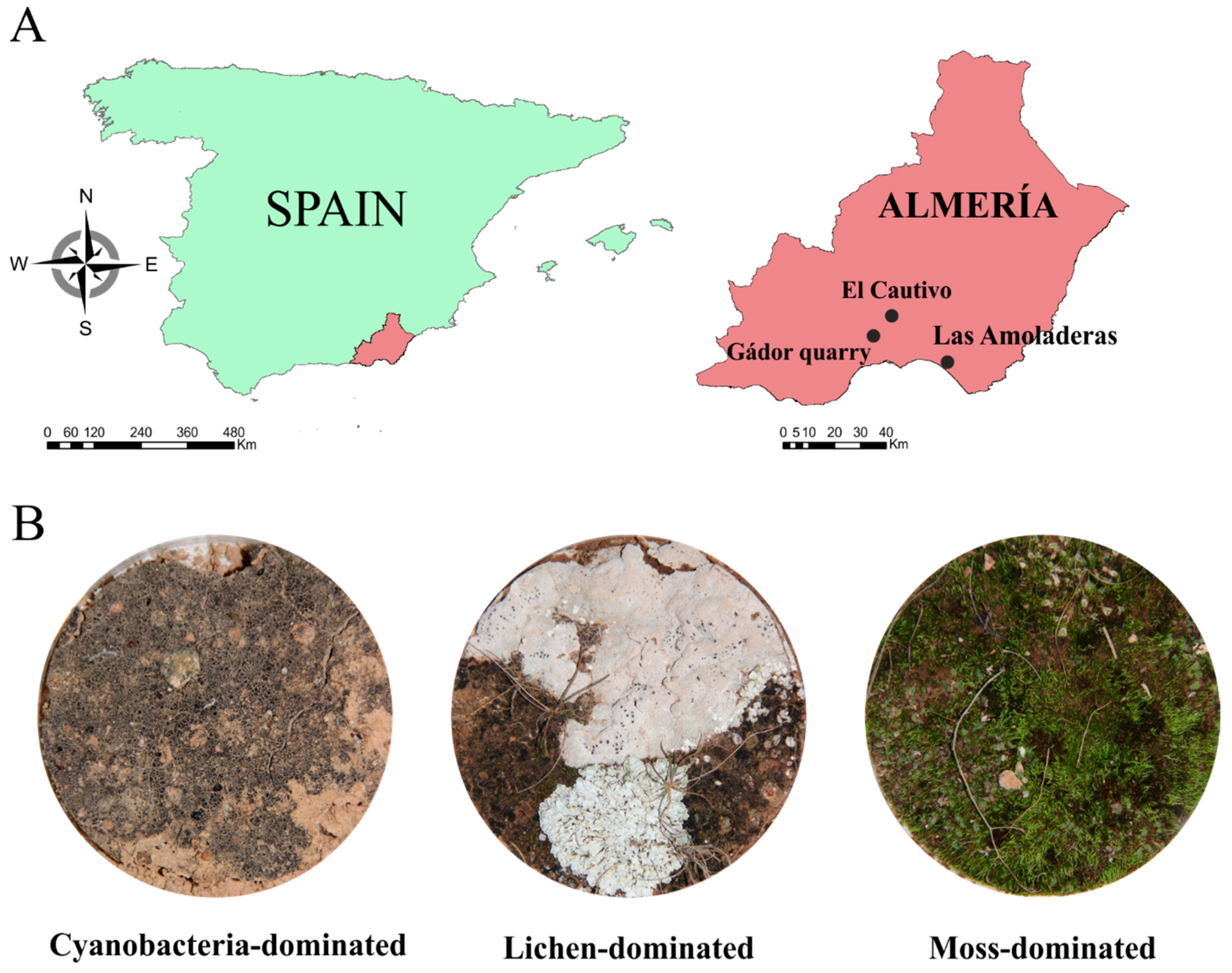
2.1. Sample Collection

Selected with contrasting differences in soil composition and color (Supplementary Table S1), a total set of 93 samples of natural biocrust communities were collected from three semiarid experimental areas within the province of Almeria (Spain) (Figure 1): (i) Las Amoladeras, within the Cabo de Gata-Níjar Natural Park (N 36° 50′ 01” W 02° 15′ 08); (ii) El Cautivo experimental area, within the Tabernas Desert (N 37° 00′ 37” W 02° 26′ 30”); and (iii) a calcareous quarry in Sierra de Gádor (W 36° 55′ 20′’ 02° 30′ 29′’ W). The mean annual rainfall and temperature in the selected areas ranges from 200–242 mm and from 17.2–19 °C, respectively.
Las Amoladeras is a semiarid steppe dominated by the alpha grass species Macrochloa tenacissima (L.) Kunth (= Stipa tenacissima L.) and sandy loam soils with a 10YR 4/6 color (dry). Most of the open spaces between plants are covered by three main biocrust types that together represent more than 30% of the total area: (a) cyanobacteria-dominated biocrust, composed of well-developed communities of cyanobacteria along with some dark lichens; (b) lichen-dominated biocrusts, mostly Diploschistes diacapasis (Ach.) Lumbsch and Squamarina lentigera (Weber) Poelt; and (c) moss-dominated biocrusts that also contain a small proportion of cyanobacteria (≈15%) (see Chamizo et al., 2012 [8] for further details).
El Cautivo is a badlands landscape developed on Tortonian gypsiferous mudstones with silty loam textured soils [54] that have a 2.5Y 6/3 color (dry). The vegetation is mainly M. tenacissima that grows along with other dwarf shrubs and a dense layer of biocrust mainly dominated by two different types: (a) cyanobacteria-dominated biocrusts that also contained numerous pioneer lichens, and (b) lichen-dominated biocrusts mainly composed of the light-colored Diploschistes diacapasis and Squamarina lentigera [55]. Moss-dominated biocrusts are also representative in some topographical positions, such as in the steep northern aspect hillslopes where low incoming solar radiation levels maximize water availability. A detailed description of the area can be found in Cantón et al., 2003 [54].
The third study site (Gádor limestone quarry experimental area), described in Luna et al., 2018 [56], was chosen as an example of a highly degraded ecosystem where biocrusts are present in an early successional stage. The soil texture in the area is clay loam with a 2.5Y 8/3 color (dry). Two main biocrust types were identified at this site: (a) cyanobacteria-dominated biocrusts, mostly incipient cyanobacteria mixed with small, dark pioneer lichens including Collema sp.; and (b) moss-dominated biocrusts in spaces close to the shrub patches in undisturbed areas.
From each biocrust community described at the three different sites (cyanobacteria-dominated biocrust from Las Amoladeras, El Cautivo, and Gádor quarry; lichen-dominated biocrusts from Las Amoladeras and El Cautivo; and mosses-dominated biocrust from Las Amoladeras, El Cautivo, and Gádor quarry), a minimum of 12 replicates, representing different compositions and coverage values, were collected between 5–7 December 2017. Before sampling, the crust coverage and composition was visually estimated and samples were selected representing different compositions and coverage values. For sampling, a 90 mm (diameter) per 15 mm (depth) Petri dish was used. The Petri dish was pressed 15 mm deep into the soil, a spatula was pushed underneath, and then both were pulled out and the Petri dish was sealed with the cap. Then, samples were transported to the University of Almería, air dried, and stored at room temperature at low light intensities for less than one week until the surface spectra and chlorophyll a extraction measurements were conducted.
At the same experimental areas, soil substrates were collected at a 2 cm depth, air-dried, and sieved to 2 mm in order to remove the small herbs and rock fragments. Three native filamentous nitrogen-fixing cyanobacteria species, Nostoc commune (CANT2 UAM 817), Scytonema hyalinum (CAU6 UAM 820), and Tolypothrix distorta (CANT7 UAM 825) that had been previously isolated from undisturbed biocrusts [57] and cultured ex situ were inoculated separately and in a mixture (1:1:1) onto Petri dishes containing soils from the three different study sites. Furthermore, non-inoculated samples from each soil type were set to serve as a control (hereafter “bare soil”). A total set of 119 inoculated soils were placed in a Fitotron Plant Growth Chamber (University of Almería, Almería, Spain) at a constant temperature (25 ± 1 °C) and a light intensity of 60 μmol photons m−2 s−1 with a 16 h photoperiod for 90 days before the spectral and chlorophyll a measurements were conducted (see details in Román et al., 2018 [58]).
Combining all these samples, we obtained a final dataset of 212 samples (93 natural and 119 artificially induced) that represented a wide range of biocrust coverage and developmental stages in different soil types with contrasting spectral properties.

2.2. Spectral Measurements and Biocrust Coverage Estimation

Thirty minutes before the spectral measurements, all samples were irrigated with 30 mL of distilled water. Next, the surface reflectance of each sample was measured using an ASD FieldSpec® Handheld portable spectroradiometer (ASD Inc., Boulder, CO, USA) with a 3.5 nm optical resolution from 325 nm to 1075 nm. All measurements were conducted in stable light conditions provided by two 14.5 V, 50 W ASD Pro Lamp (ASD Inc., Boulder, CO, USA) halogen lamps, with the optical fiber placed 16 cm above the sample surface, resulting in a field-of-view (FOV) area of 66 cm2 corresponding to the entire surface of the Petri dish. A total of three replicate measurements, each consisting of the average of the three individual spectra, were collected for each sample and then averaged to produce the sample surface spectrum. A Spectralon (ASD Inc., Boulder, CO, USA) white reference sample was also measured before each set of three biocrust spectra.
In addition, after the spectral measurements, a zenithal picture of each sample was acquired using a digital Canon EOS 600D (Canon Inc., Tokyo, Japan) placed at nadir, 25 cm above the sample surface. Then, the biocrust coverage (%) on the soil substrates was calculated using the supervised maximum likelihood classification in the ENVI 4.7 software (ITT VIS, Boulder, CO, USA).

2.3. Chlorophyll a Extraction

After the spectral measurements, a 3-mm thick biocrust subsample was collected from each Petri dish for determining the biocrust chlorophyll a concentrations (Chla). Samples were air-dried at ambient temperature, crushed with a roller, and then ground with a mechanical agate mortar. Chlorophyll a extraction from soil samples was conducted by following the ethanol double-extraction method developed by Castle et al., 2011 [25]. The supernatants from both extractions were combined and the absorbance was measured at 649, 665, and 750 nm. As the inoculated soils were only comprised of cyanobacteria-inoculated strains, a specific equation developed by Ritchie, 2006 [59] for these organisms was applied in order to calculate Chla, as follows:
Chla   ( μ g / g   soil ) = ( 11.9035 × A ( 665 750 ) × V ) ( g   soil × L )
where the absorbance coefficients have the dimensions μg∙cm/mL∙A, A is the absorbance value at the specific wavelength, V is the volume of the extract (mL), and L is the optical path length of the spectrophotometer cuvette (cm).
For natural biocrust communities, comprised of a mix of different photoautotrophic organisms, Chla was calculated by applying the equation for chlorophytes and bryophytes reported by Ritchie, 2006 [59] (Equation (2)):
Chla   ( μ g / g   soil ) = ( 13.5275 × A ( 665 750 ) 5.201 × A ( 649 750 ) ) × V ) ( g   soil × L )
where the absorbance coefficients have the dimensions μg∙cm/mL∙A, A is the absorbance value at the specific wavelength, V is the volume of the extract (mL), and L is the optical path length of the spectrophotometer cuvette (cm).

2.4. Spectral Data Analysis

Before the spectral analyses, all data were subjected to a pre-treatment that consisted of removing the noisy bands (350–400 nm and above 950 nm) and applying a cubic polynomial smoothing filter with a 17-nm window size [60]. Moreover, all spectra were resampled to a Sentinel-2 multispectral resolution, which included broad bands at the blue (490 nm), green (560 nm), red (665 nm) and near-infrared (NIR, 842 nm) regions of the spectra, as well as some narrower bands within the red edge region (740, 783, and 865 nm). This procedure was done by applying the spectral resampling functions included within the “hsdar” package in R version 3.3.3 (R-project; [61]).

2.4.1. Data Transformation

As the reflectance at a single determined wavelength (R) is very sensitive to variable irradiance, background effects, and the geometric arrangement of the sensor and surface [62], we explored the usefulness of well-known spectra transformations that have proven to be very useful for isolating the particular absorption features of different pigments, such as the continuum removal (CR; [63,64]) and the first derivative of the spectra (ρ; [65,66,67]). The CR and ρ were calculated for each biocrust type using the pre-treated spectra from 400 to 950 nm by 1 nm. The CR was calculated by applying the convex hull fit over the top of a spectrum using straight-line segments that connect the local spectra maxima so that values equal to 1 indicate the absence of absorption peaks (the spectrum matches the convex curve), while values lower than 1 indicate the presence of absorption peaks [63]. The ρ was calculated using the Savitzky and Golay [60] method with third-order polynomials and a 17-nm window size, based on previous exploratory analysis. We also estimated the band depth (1- CR; BD) for the complete 212-sample dataset and from this we calculated several well-known spectral properties related to two main chlorophyll spectral absorptions at 460 nm and 680 nm including: (i) the area under the absorption peak (area), (ii) the maximum absorption value (max), (iii) the wavelength at which maximum absorption is observed (maxwl), (iv) the wavelength positions of upper and lower half-max values (up-wlhm and lo-wlhm), (v) the difference between wavelength positions of upper and lower half-max values (width wlhm), and (vi) the root mean square error (RMSE) between a Gaussian distribution function and the feature values between the lower half-max and the maximum position and between the upper half-max and the maximum position (gaus-low wlhm and gaus-up wlhm). All analyses were done using the “hsdar” package in R (R-project; [61]).

2.4.2. Band Ratios and Standard Spectral Indexes

Biocrust spectra at hyper- and Sentinel-2 multispectral resolutions were also used to calculate the normalized difference indexes (ND) for all possible band combinations between 450–900 nm, following Equation (3):
ND = ( RB 1 RB 2 ) ( RB 1 + RB 2 )
where ND is the normalized difference index between bands 1 and 2, and RB1 and RB2 are the reflectance values at spectral bands B1 and B2, respectively.
Finally, a set of 38 existing published Chla-related narrow- and broad-band vegetation indexes were also calculated for each sample (Supplementary Table S2). The selected indexes were chosen from previous studies that reviewed leaf chlorophyll quantification from spectral information [36,67,68]. Specific details about the formulations and reference sources are summarized in Supplementary Table S2.

2.5. Statistical Analysis

The differences in Chla between the different biocrust types and sample sites were analyzed using the two-way analysis of variance (ANOVA) and Tukey’s honestly significant difference (HSD) post hoc test. Moreover, a linear regression analysis was performed to explore the relationships between Chla concentration and R, CR, and ρ values of different bands of the spectrum, as well as the relationships between Chla and all possible ND and standard vegetation indexes. This was repeated for the complete 212 sample dataset and for each crust type separately: (i) artificially induced cyanobacteria biocrusts (“inoculated”) on soils from Las Amoladeras, El Cautivo and Gádor quarry; (ii) natural cyanobacteria biocrust communities (“cyanobacteria-dominated”) from Las Amoladeras, El Cautivo, and Gádor quarry; (iii) lichen biocrusts (“lichen-dominated”) from Las Amoladeras and El Cautivo; and (iv) mosses biocrust (“moss-dominated”) from Las Amoladeras, El Cautivo, and Gádor quarry. For all regression models, the differences between predicted values and observed values was assessed using the root mean squared error (RMSE) and the coefficient of determination (R2) of the chlorophyll quantifications were estimated.
Finally, we developed a random forest (RF) multivariate model for Chla estimation, which is applicable to a wide range of biocrust coverage and compositions using all spectral properties derived from the two main Chla absorption features corresponding to the first two peaks of the BD values (at 460 nm and 680 nm). To do this, we used the complete dataset in a 20-fold cross-validation strategy. Moreover, in order to test the influence of biocrust coverage on our Chla estimations, we repeated this model also considering the coverage of incipient cyanobacteria, well-developed cyanobacteria and some pioneer lichens such as Collema cristatum (L.) F.H. Wigg, Endocarpon pusillum Hedw, Fulgensia fulgida (Nyl.) Szat, and Fulgensia desertorum (Tomin), lichens, and mosses. The number of predictor variables performing the data partitioning at each node and the total number of trees to be grown in the model run were set to 20 and 100, based on a previous tuning experiment. Model fit was tested using the mean RMSE obtained during the cross-validation process, and importance of predictor variables was measured using the Gini decrease in node impurity measure, which is computed by permuting the predictor variables with the out-of-bag data in the RF validation approach (details in Liaw and Weiner, 2002 [69]). Finally, in order to get an estimation of linear fit between estimated versus measured Chla concentrations that were comparable with this obtained by linear regression, we applied the obtained RF model to the complete dataset.

3. Results

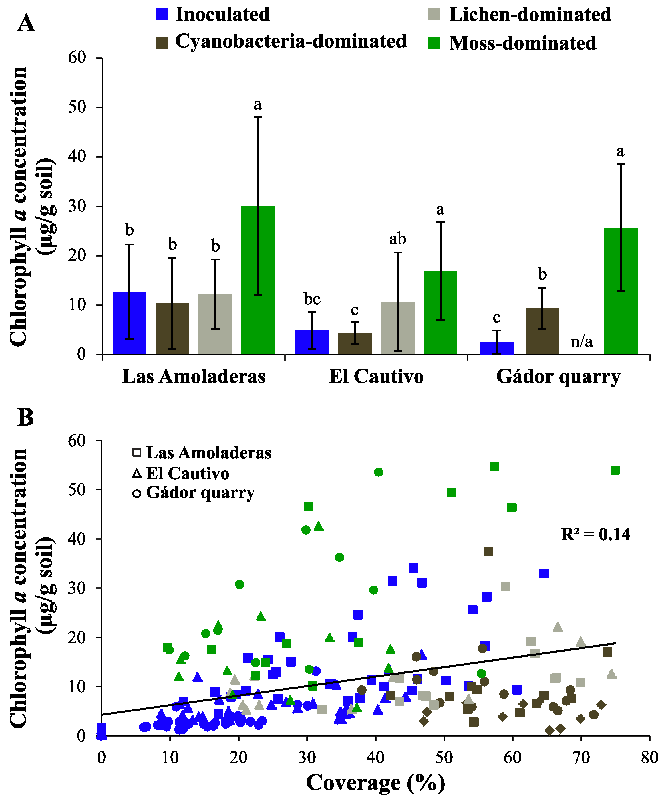
3.1. Chla of Different Biocrust Types

From the different natural biocrust types considered in this study, the moss-dominated biocrusts showed the highest Chla amongst the three different study sites. The values ranged from 8 µg/g soil in the moss samples with a surface coverage below 28%, to 54 µg/g soil on fully covered samples from Las Amoladeras (Figure 2). The lichen-dominated biocrusts showed intermediate values (from 5.28–30.31 µg/g soil), whereas cyanobacteria showed the lowest values amongst the three different sites (from 1.22–38.94 µg/g soil). However, the differences between cyanobacteria- and lichen-dominated biocrusts were not significant as a consequence of the large variability in coverage and chlorophyll concentrations amongst the different samples (Figure 2). The Chla of the 119 artificially inoculated cyanobacteria (three months old) samples ranged from 0–34.05 µg/g soil. The highest values corresponded to cyanobacteria inoculations on soils from Las Amoladeras that showed very similar values to those found in natural cyanobacterial biocrust communities, whereas the artificially induced cyanobacterial biocrusts on the quarry substrates showed the lowest Chla amongst all the samples analyzed in this study (Figure 2).

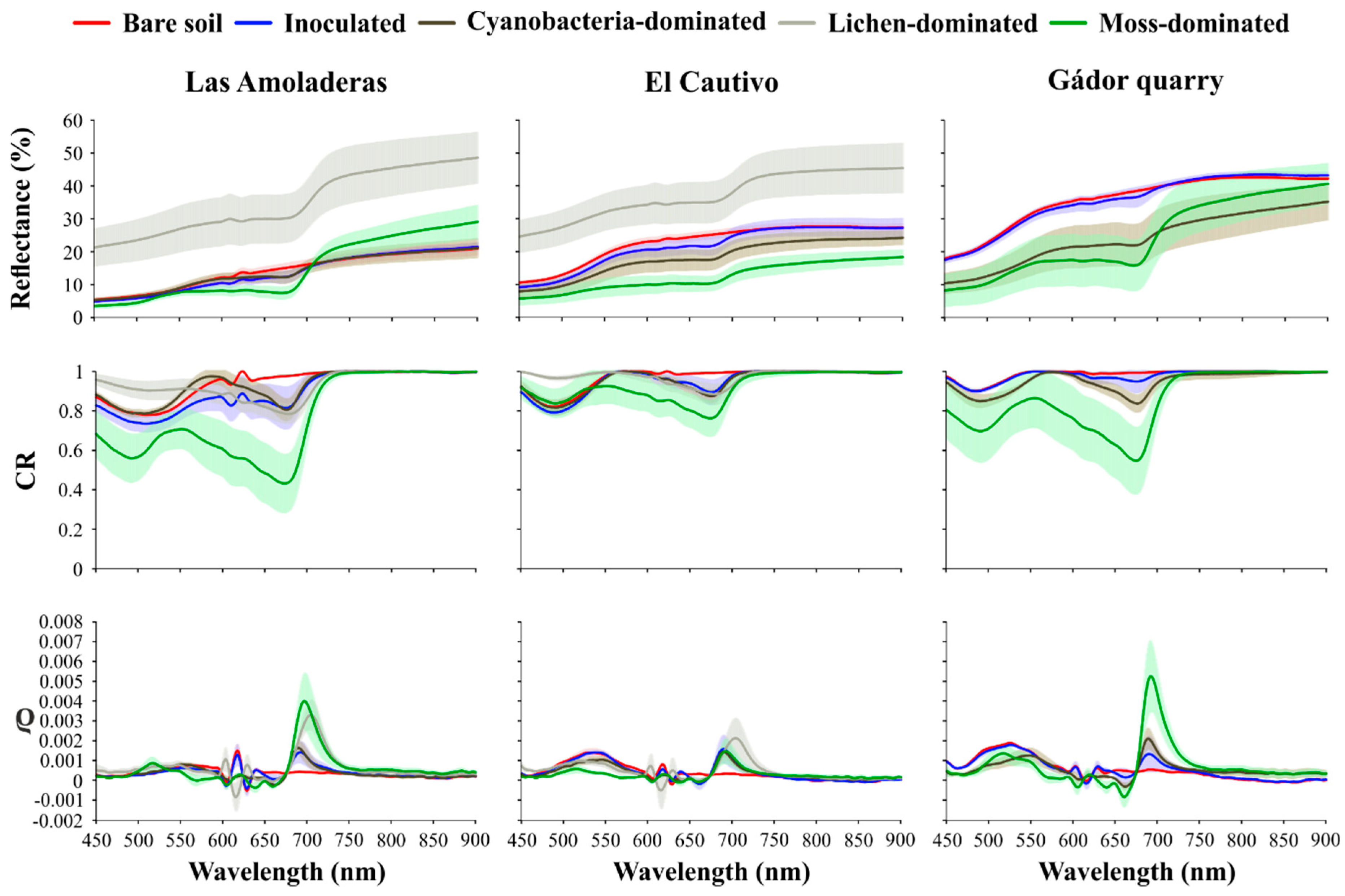
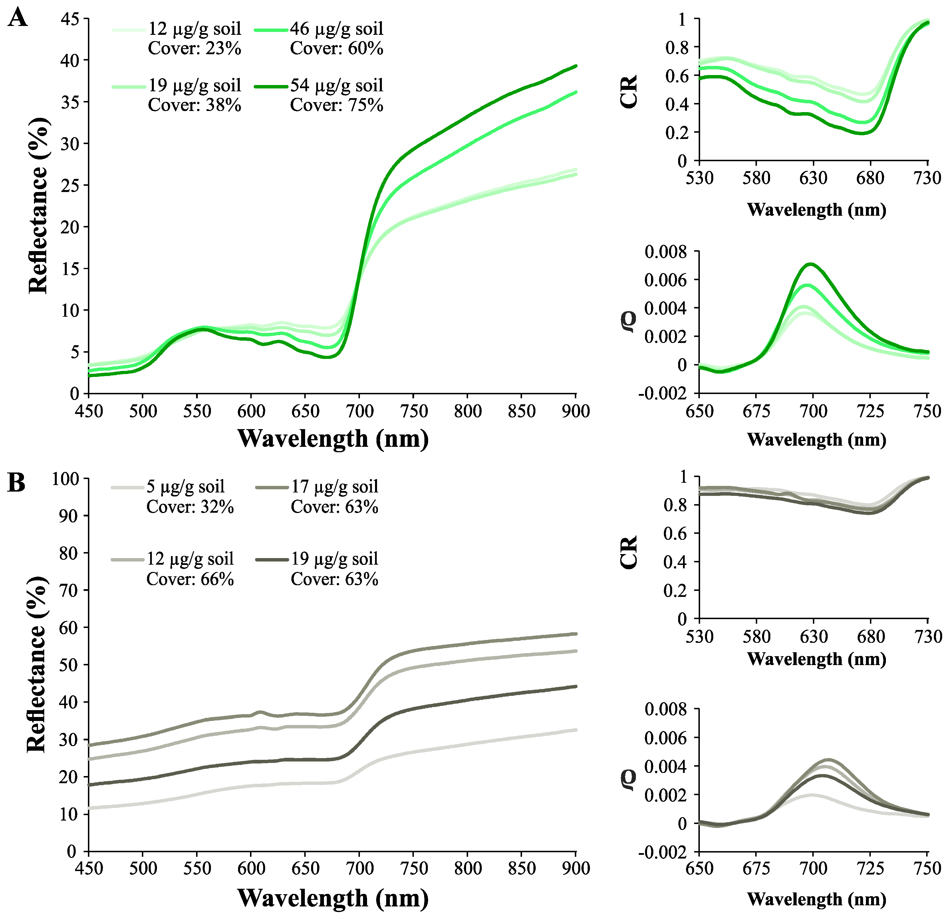
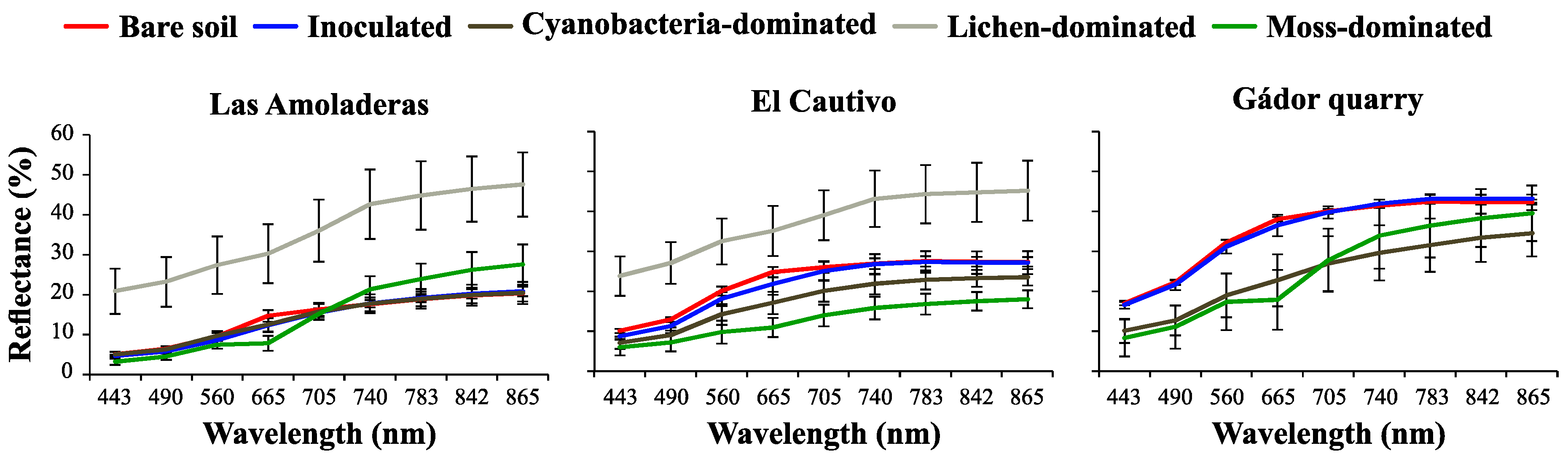
3.2. Effect of Biocrust and Chla on the Soil Surface Spectra

Figure 3 shows the mean reflectance, CR, and ρ of the different natural biocrust communities from the three different study sites, as well as the values of the spectral variables for the artificially induced cyanobacterial biocrusts on the soils from the three sites. Overall, the biocrust samples dominated by white lichens showed higher reflectance values than the bare soils, whereas the moss- and natural cyanobacteria-dominated crusts showed the opposite effect (Figure 3). The artificially inoculated cyanobacteria biocrusts also produced a slight decrease in the overall surface reflectance of the three different reference soils, but this effect was lower than the effect from the natural communities (Figure 3). There were also some important differences in the spectral shape between the bare soils and biocrusts. For example, all biocrust types showed an important absorption peak at about 670 nm that was not pronounced in the reflectance spectrum but could be easily identified in the CR, ρ, and BD (Figure 3). Overall, samples with higher biocrust coverage or Chla had a more accentuated spectral absorption with a minimum in the CR curve at 670 nm and a spike in the ρ (Figure 3), with some exceptions occurring on the lichen and natural cyanobacteria samples (Figure 4b). Subsequently, this spectral absorption was more pronounced on the moss-dominated biocrusts than on the lichen, cyanobacteria, and artificially inoculated cyanobacteria biocrusts (Figure 3), exhibiting a similar pattern to the Chla. Another important spectral absorption at about 500 nm was identified from the CR and ρ of the moss, cyanobacteria, and bare soil samples that was masked in lichen-dominated biocrusts. When the spectral signatures of the different biocrusts were resampled to Sentinel-2 multispectral resolution, the spectral curves showed a similar shape, but differences were subtler than those observed at a hyperspectral resolution (Figure 5).

3.3. Chlorophyll a Predictions

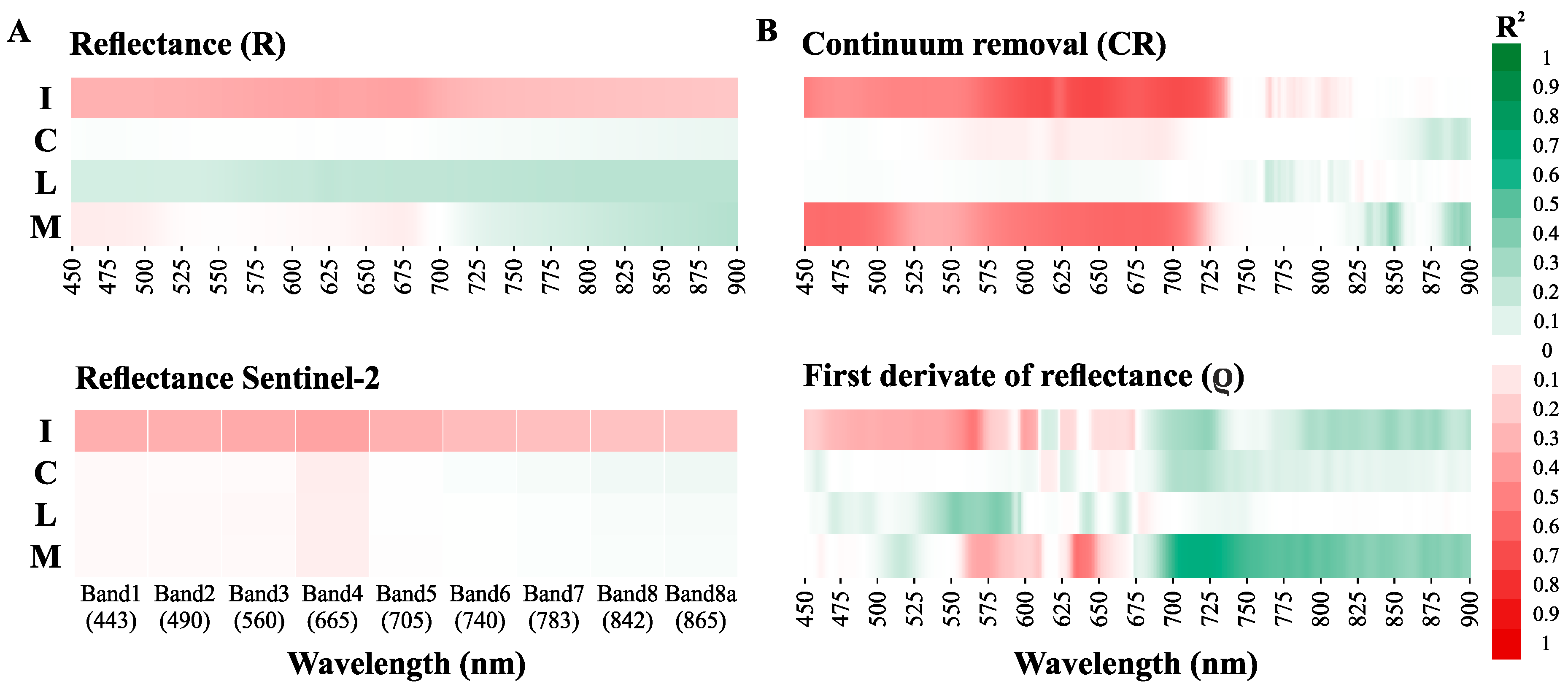
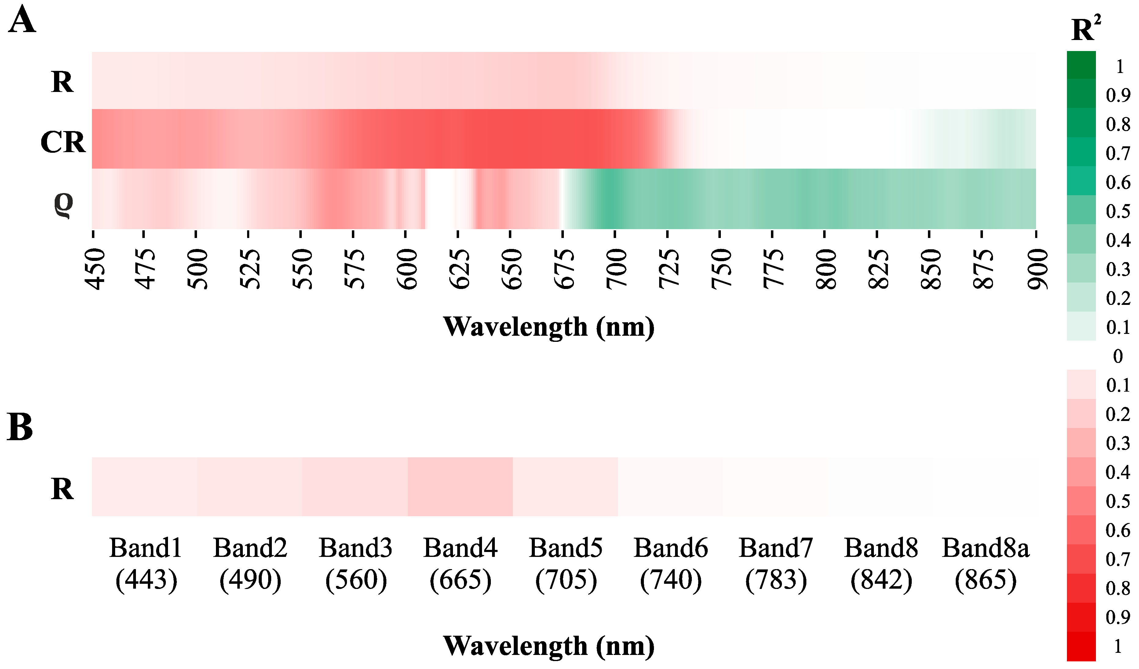
3.3.1. Direct Chla Predictions from the Surface Reflectance, CR, and ρ

The relationships between the biocrust spectra and Chla are shown in Figure 6. Overall, hyperspectral information provided more accurate results in Chla predictions than multispectral data, as shown by slightly higher values of the coefficient of determination and lower RMSE (Figure 6, Table 1). The soil surface reflectance within the Vis-NIR region decreased as Chla increased, with the best regression coefficient found at about 674 nm (Figure 6, Table 1). However, the regression fits were very low at both multi- and hyperspectral resolutions (R2 = 0.21 and 0.19, respectively). The CR in the red region and ρ transformation showed a better relationship with Chla than surface reflectance, yielding a coefficient of determination of up to 0.68 and 0.51, respectively. Overall, the CR values decreased as Chla increased, with the best regression fits between CR and chlorophyll observed at 655 nm (Figure 6, Table 1). On the other hand, ρ showed the best regression fits with spectral bands at the inflection point of the red-edge (about 700 nm).
When the different biocrust communities were analyzed separately, we found that the correlation patterns between the surface reflectance, CR, and ρ and Chla strongly varied amongst the biocrust communities (Figure 7a,b). Whereas the CR within the red region showed the best correlation with Chla on the artificially induced cyanobacteria biocrusts (646 nm, R2 = 0.71), and ρ at the inflection point of the red edge showed the best results on the moss and natural cyanobacteria dominated biocrust communities (723 nm and R2 = 0.65, and 720 nm and R2 = 0.27, respectively) (Figure 7b, Table 1). Chla within the lichen-dominated biocrusts best fit to the ρ values within the green region of the spectra (581 nm, R2 = 0.41).

3.3.2. Chlorophyll a Predictions from the Normalized Band Ratios

The normalized band combination ratios were as sensitive to chlorophyll changes as CR and ρ at both the hyperspectral and Sentinel-2 multispectral resolutions (Table 1). For example, when all biocrust samples were analyzed together, the best fits were obtained by combining the chlorophyll absorption band at 687 nm and the reflectance from 731–736 nm for the hyperspectral data, and band 4 and band 5–6 for the Sentinel-2 spectral resolution, yielding a coefficient of determination of 0.69 (Table 1; Supplementary Figures S5 and S10). However, similar to the results found when the Chla-R, CR, and ρ regressions were analyzed, the best band selection and overall fit strongly varied between the crust types. For artificially inoculated cyanobacteria, the best results were obtained using the combination of the surface reflectance at 704 nm (band 5 of Sentinel-2) and the surface reflectance at 730 nm (band 6 of Sentinel-2), yielding a coefficient of determination of about 0.72 (Table 1; Supplementary Figures S1 and S6). The moss chlorophyll showed a better correlation with band ratios based on spectral reflectance at 518 and 519 nm, yielding a coefficient of determination of 0.65. However, these subtle spectral traits were not correctly characterized at the Sentinel-2 spectral resolution, at which the best correlation was found using band 4 and bands 5–6 (R2 = 0.62) (Table 1; Supplementary Figure S9). Band ratios within the red or NIR regions were not sensitive to changes in Chla in the natural cyanobacteria-dominated crusts that showed the best relationship with band ratios combining the surface reflectance at 466 nm and 455 nm (Table 1; Supplementary Figure S2). As previously shown for R, CR, and ρ, the absolute values were again very low (R2 = 0.26). On the lichen-dominated biocrust samples, no significant relationship was found between the normalized bands and Chla for most bands. In these crusts, only the region around 680 nm showed a poor relationship with Chla (R2 = 0.19; Table 1; Supplementary Figure S3).

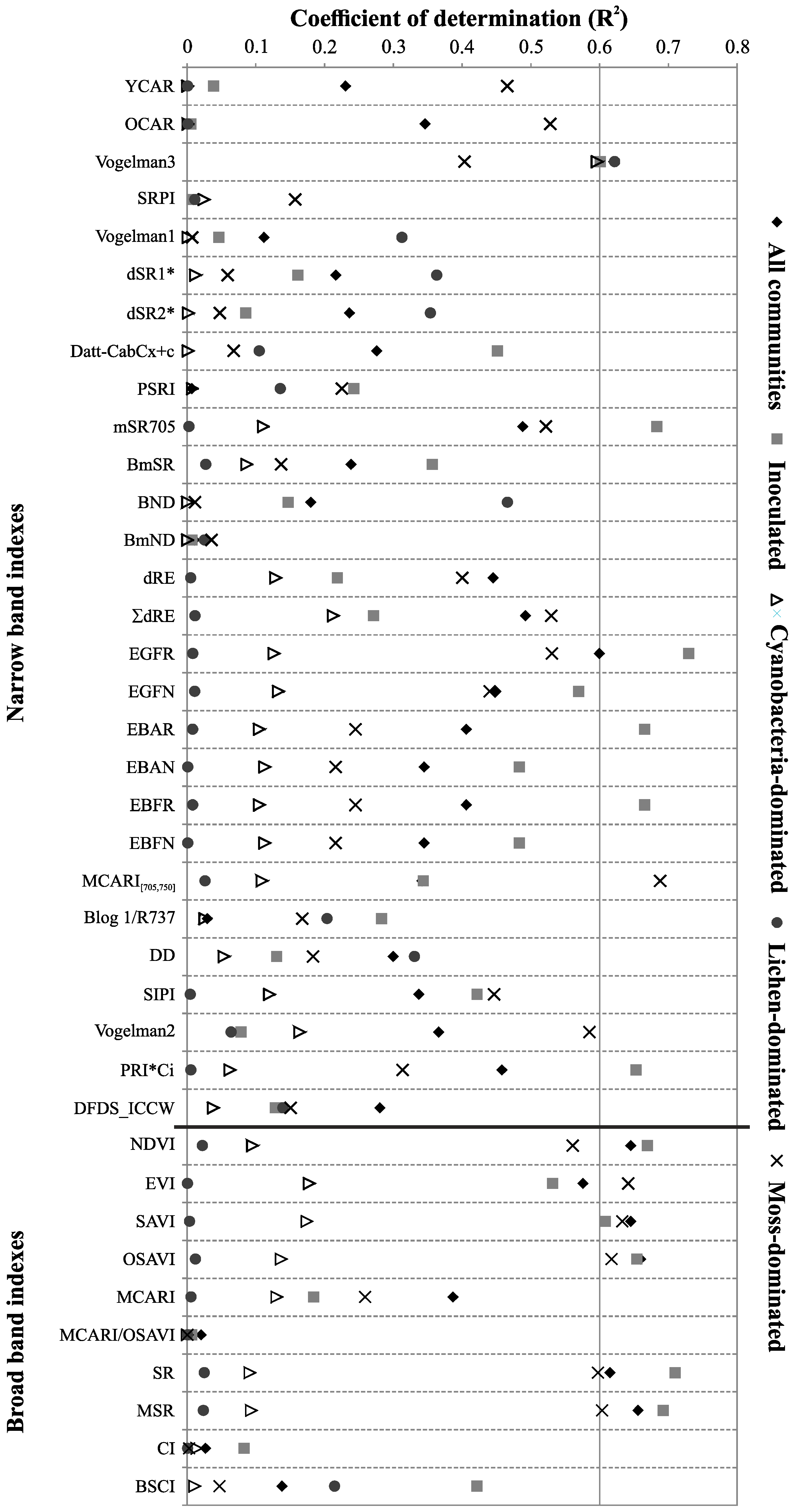
3.3.3. Sensitivity of the Standard Spectral Indexes to the Chlorophyll a Determination

Similar to the normalized band ratios, the standard spectral indexes also were sensitive to changes in the biocrust chlorophyll concentration. Of the 28 narrow band and 10 broad band spectral indexes (Supplementary Table S2), 6 were robustly sensitive to the biocrust Chla (R2 > 0.6; Figure 8). The best retrievals for the general biocrust communities (all samples) were provided by the broad band greenness indexes using red and NIR information, such as the NDVI, simple ratio (SR), modified simple ratio (MSR), soil adjusted vegetation index (SAVI), and the optimized soil-adjusted vegetation index (OSAVI), yielding a coefficient of determination above 0.6 at both the hyper and Sentinel-2 spectral resolutions (Figure 8, Table 1). Biocrust specific indexes crust index (CI) and biological soil crust index (BSCI), on the other hand, did not provide good results.
The broad band greenness indexes also appeared to be good predictors of Chla for the artificially induced cyanobacteria and the natural moss biocrust samples. However, when these biocrust types were analyzed separately, some narrow band pigment-related indexes, such as the modified chlorophyll absorption in reflectance index (MCARI[705,750]) (for mosses) and the ratio of first derivative maxima in red-edge region and green region (EGFR) (for artificially induced cyanobacteria) showed better relationships with the chlorophyll concentrations than the broad band indexes, yielding coefficients of determination up to 0.69 and 0.72, respectively. In the case of the lichen-dominated biocrusts, only the narrow band normalized band ratio between 700–722 nm (BND; [67]) showed a good fit, whereas none of the narrow or broad band ratios fit well with Chla on the natural cyanobacteria-dominated biocrusts.

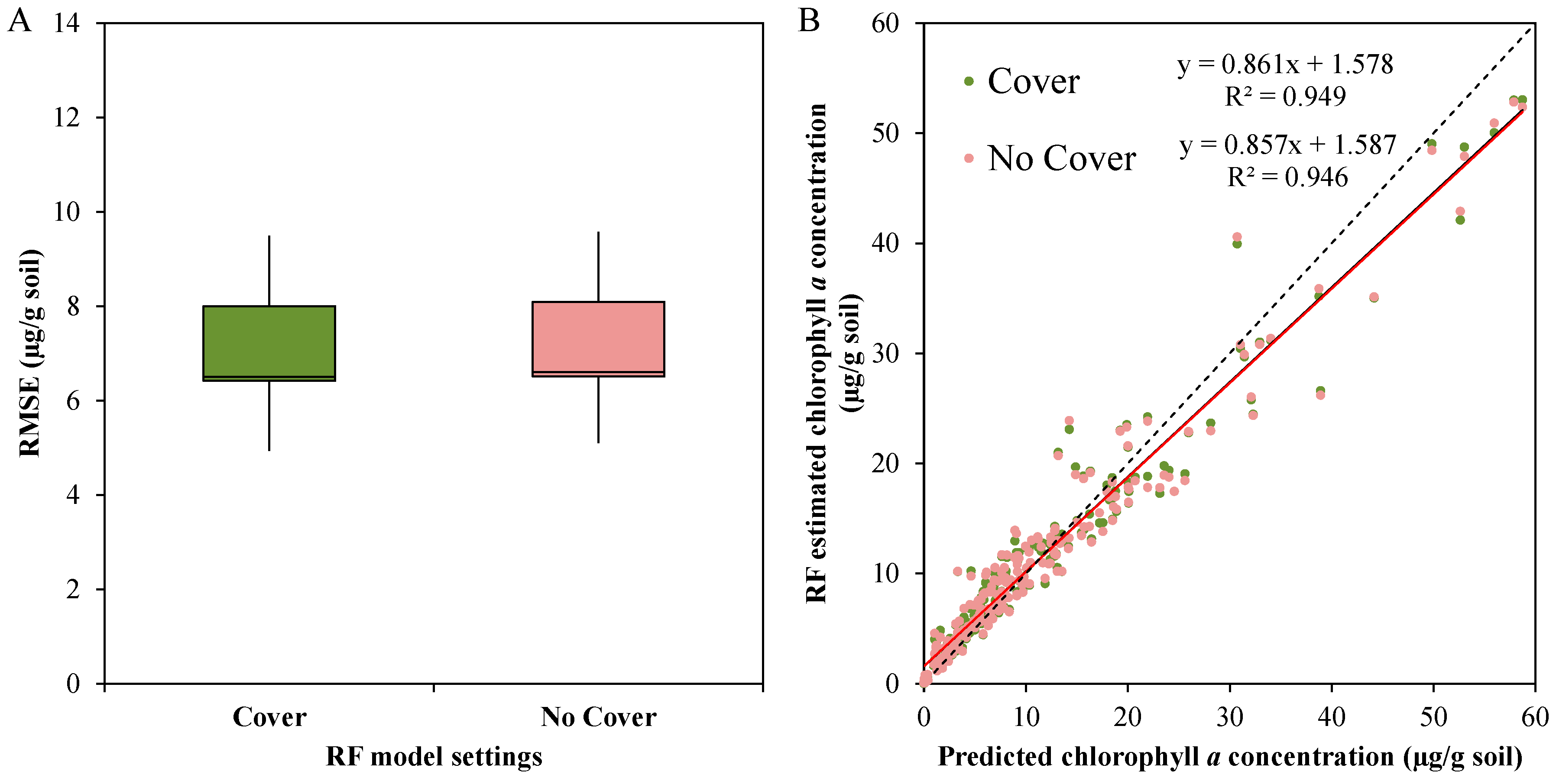
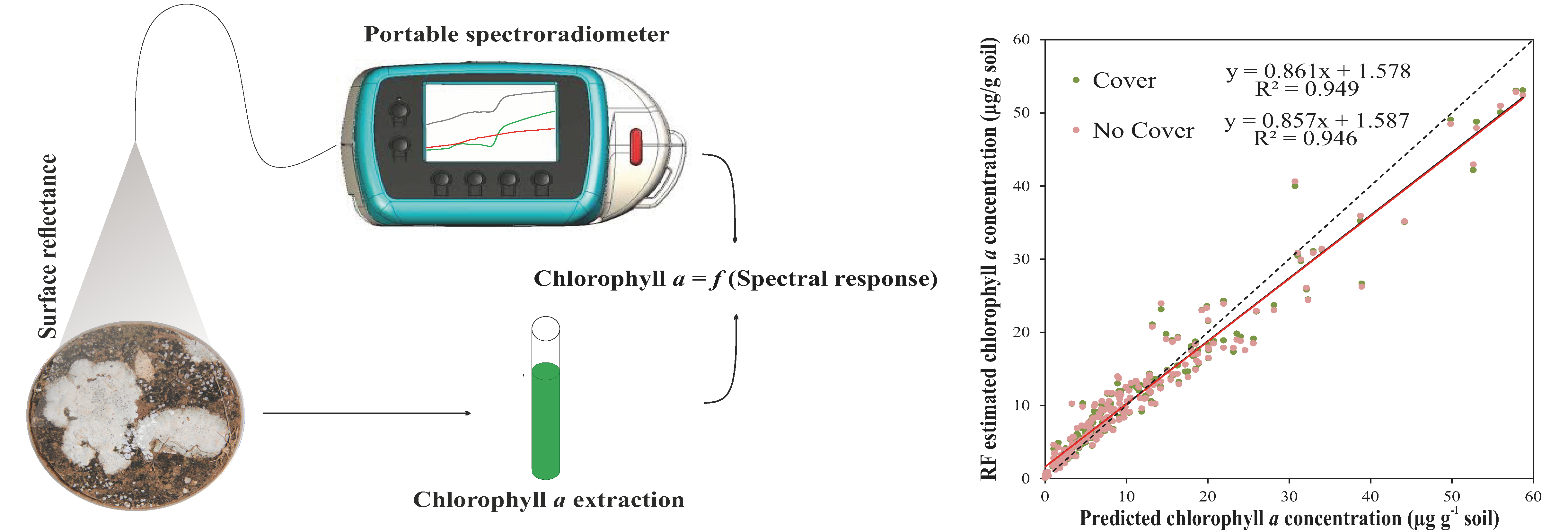
3.3.4. General Random Forest Model for Chla Prediction over a Wide Range of Biocrust Coverage and Composition Values

Figure 9 summarized the results of the random forest model performance. Overall, both RF models (the model that exclusively considered spectral properties derived from the two main absorption peaks and the RF model also including biocrust coverage) provided a very good fit with a mean RMSE about 6.5 µg/g soil. Moreover, when they are applied to the complete dataset, in order to get an accuracy estimation comparable with that obtained using linear regression, the prediction accuracy increased (coefficient of determination between predicted and observed Chla values = 0.95; Figure 9). The three most important predictor variables for Chla estimation in both models were maximum depth within the 680 nm absorption peak, gaus-low wlhm, and gaus-up wlhm, whereas the coverage of the different biocrust components played only a secondary role (Supplementary Figure S11).

4. Discussion

Chla provides valuable information about the photosynthetic capacity of biocrusts [27] and have been widely used as a surrogate for biocrust development and growth of both natural and artificially induced biocrust communities [15,28,58,70,71]. However, until now, most analyses were based on punctual measurements and required destructive sampling that hindered the analysis of seasonal dynamics and growth rates in these spatially heterogeneous communities during long term monitoring experiments. The present study demonstrates that natural and artificially induced biocrust communities present certain common spectral traits related to the presence of chlorophyll that, although less accurate than traditional laboratory analyses, represent an alternative non-destructive and reliable method to quickly quantify Chla and biocrust development.
The spectral analysis of our experimental dataset corroborated that, according to several studies analyzing different biocrust communities around the world [2,48,49,50,51,52], biocrusts modify soil surface reflectance with a main absorption detected in the reflectance red peak at about 680 nm, and along the red edge (Figure 3) that corresponds to the well-known chlorophyll a spectral absorption [72,73,74,75]. However, contrary to previous studies [2,76], we found that the use of single band reflectance values at this wavelength were not able to accurately estimate Chla of biocrust communities, as shown by the lower coefficient of determination and higher RMSE values obtained compared to those obtained with the ρ, CR, ND, and standard spectral indexes (Table 1). This may be due to the fact that our dataset was composed of different biocrust communities dominated by a variety of phototrophic organisms with different spectral traits [2,50] that, as previously reported by Escribano et al., 2017 [77], interact with the soil reflectance in multiple ways, modifying the final reflectance values independently of the biocrust chlorophyll concentration. For example, whereas dark cyanobacteria- and green moss-dominated biocrusts reduced the overall soil surface reflectance when compared to the bare soil spectra, white lichens that occur in the experimental zones caused the opposite effect, especially in the dark-colored soils from Las Amoladeras (Figure 3). A chlorophyll-a-related absorption peak at about 680 nm was enhanced by the biocrust spectra normalization using the CR and ρ spectral transformations. In this study, all biocrust types showed a deep absorption peak in the CR spectra at about 670 nm and a subsequent spike at 700 nm in the ρ spectra (Figure 3). CR and ρ are commonly used to isolate particular absorption features because they are less sensitive to differences in the overall reflectance and color between different samples [36,64,66] and they have been found to be a good predictor of Chla in plants and leaves [64,65,66,78,79]. However, previous studies on natural biocrust communities that described this chlorophyll-related spectral feature were focused on identification and mapping (see Weber and Hill, 2016 [2] and references within) and thereby did not explore the potential of the CR and ρ to quantify biocrust Chla. We found that absorption values within the red and the red-edge spectral region extracted from the CR and ρ normalization, respectively, improved chlorophyll a estimations when compared with reflectance values, yielding a coefficient of determination above 0.6 (Figure 6). Moreover, the depth of the absorption peaks increased from the very incipient artificially induced cyanobacteria-dominated biocrust to the well-developed, moss-dominated biocrusts as Chla increased (Figure 3), highlighting the potential of spectral transformations to be used as an alternative biocrust development index.
Normalized difference band ratios including the red and NIR spectral bands, as well as the standardized broad- and narrow-band spectral indexes using the same spectral information (e.g., MSR, OSAVI, NDVI, SAVI), were also strongly correlated with the biocrust Chla, giving a similar prediction accuracy as the CR and ρ spectral transformations (Table 1). Thus, results obtained two decades ago by Karnieli et al., 2001 [53] who found a good relationship between the NDVI value of biocrust communities representing different levels of development and chlorophyll, are now confirmed for a dataset composed of 212 samples from different ecosystems that comprised a wide range of biocrust coverage and compositions with chlorophyll a values that varied from 0–54.63 µg/g soil on different soils with contrasting soil textures and physicochemical properties, and thus, spectral properties. This approach may reduce the obtained accuracy in comparison with local applications that only considered one soil or biocrust type, but it increases the transferability of the results to a wider range of applications that consider different soil types and biocrust compositions (including monitoring, analysis and comparison of natural biocrust dynamics, and artificially induced biocrust communities).
The good relationships found between the hyperspectral data and Chla are promising and suggest that the best indexes found in this study (Table 1) can be used for reliable estimations of biocrust Chla. Moreover, in a similar way as Chla, spectral absorption at 670 nm and the value of the different spectral indexes values increased as biocrust development did. This positive relationship allowed us to propose biocrust reflectance as a quick, cheap, and non-destructive sampling method to monitor biocrust development over long-time spans, with several potential applications for field and laboratory studies. Furthermore, the good results obtained with the use of hyperspectral information denote a high potential of space-based hyperspectral imagery, as the already launched DESIS or PRISMA hyperspectral missions [80] or several upcoming missions, such as EnMAP and HySPIRI, with hundreds of spectral channels covering the RED and NIR regions with a high potential for biocrust monitoring and biomass retrieval over a wide variety of locations and scenarios. Of note are also the good results obtained by the application of broad band greenness indexes, yielding models that were as reliable and accurate at predicting Chla as those obtained at hyperspectral resolution (Figure 8). The good fits obtained via the application of broad band greenness indexes at the Sentinel-2 multispectral resolution, combined with the high temporal and spatial resolution that characterize this satellite, open a wide range of opportunities for biocrust monitoring at regional scales that would allow for their use in monitoring programs aimed at understanding biocrust responses to ongoing global change and degradation processes. However, before imaging spectroscopy can be applied in the quantification of chlorophyll a in biocrusts, more effort is needed in order to deal with additional difficulties related with atmospheric effects, shadows effects, effect of soil water content on spectral response, or interactions with other surface components such as vegetation that absorb solar radiation at similar wavelengths to biocrusts. Moreover, a specific calibration would be necessary as marked differences are found when the biocrust behaviors are analyzed separately (Figure 7a). Chla for the mosses and artificially induced cyanobacteria showed good correlations with most indexes that fit well for the whole dataset, whereas worse results were obtained for lichen-dominated biocrusts and natural cyanobacteria communities. This can be explained by several factors. To cope with high UV levels, natural cyanobacteria communities produce a wide variety of sunscreen pigments, such as scytonemins and carotenoids [81,82], that also absorb solar radiation and interact with the chlorophyll spectral absorption profile [83]. Other species, such as Microcoleus vaginatus or Oscillatoria sp., reside below the soil surface during droughts and glide upwards only during long favorable periods when soil pore water is available [84,85], a trait that reduces detection accuracy. Moreover, in dryland soils with numerous vesicular pores where solar radiation can penetrate the soil profile, recent studies revealed that high levels of activity beneath the soil surface would not be observable using remote sensing technologies [86]. In the case of lichen-dominated biocrusts, the photobiont is usually sheltered in tight fungal structures that may be difficult to detect in chlorophyll-a-related spectra. Moreover, the lichen species analyzed in this study, such as Diploschistes sp., have a rugged surface that can create an additional habitat between the thalli and the soil for other organisms, such as cyanobacteria, that cannot be observed using optical techniques. In these cases, when the chlorophyll variability is below the detection limit, accurate laboratory analyses are necessary, and other approaches such as the use of coverage values, surface albedo, or roughness could be an alternative.
As an efficient machine learning algorithm, our RF model successfully sorted out all difficulties related with spectral dissimilarities between different biocrust types and provided the most accurate estimation of all methodologies tested in this study without the need for a specific calibration for each biocrust type (Figure 9). This can be explained by the capacity of RF to model non-linear relationships [87], but also because the RF model implies the combination of Chla absorption values at a specific wavelength with other properties related with the shape and specific position of Chla absorptions that are specific to the different biocrust components (Figure 3). This represents a step toward the usability of spatially-explicit spectral information with coarser spatial resolution, such as that obtained from future satellite hyperspectral images, as they showed good transferability during the cross-validation process (Figure 9a). However, as in the case of the application of specific absorption features or vegetation indexes, more effort is needed in order to deal with the additional difficulties presented when airborne or satellite images are analyzed.

5. Conclusions

Our results demonstrate that biocrust reflectance represents a valuable alternative for non-destructive and reliable retrieval of general biocrust chlorophyll a concentration and biocrust development that could be incorporated into monitoring programs. From the different methods analyzed, spectral transformation, such as CR and ρ, as well as normalized band ratios and standard hyperspectral and broad band indexes, provided accurate results. However, such approaches should be carefully adapted to each specific case as these methods were not able to correctly predict subtle differences in chlorophyll a concentration in lichen-dominated biocrusts and natural cyanobacteria communities, and therefore, specific calibrations prior to broader application are recommended. These marked differences in the biocrust spectral behaviors can be solved by the application of RF models based on different spectral properties derived from Chla or by a combination of absorption spectral properties and coverage values.

Supplementary Materials

The following are available online at https://www.mdpi.com/2072-4292/11/11/1350/s1, Figure S1: 2-D correlation plot illustrating the coefficient of determination (R2) of the normalised difference indices for all possible band combinations between 450–900 nm at hyperspectral resolution, for cyanobacteria artificially inoculated. Only the significant values (P ˂ 0.05) are represented. Figure S2: 2-D correlation plot illustrating the coefficient of determination (R2) of the normalised difference indices for all possible band combinations between 450–900 nm at hyperspectral resolution, for natural cyanobacteria-dominated subsamples. Only the significant values (P ˂ 0.05) are represented. Figure S3: 2-D correlation plot illustrating the coefficient of determination (R2) of the normalised difference indices for all possible band combinations between 450–900 nm at hyperspectral resolution, for natural lichen-dominated subsamples. Only the significant values (P ˂ 0.05) are represented. Figure S4: 2-D correlation plot illustrating the coefficient of determination (R2) of the normalised difference indices for all possible band combinations between 450–900 nm at hyperspectral resolution, for moss-dominated subsamples. Only the significant values (P ˂ 0.05) are represented. Figure S5: 2-D correlation plot illustrating the coefficient of determination (R2) of the normalised difference indices for all possible band combinations between 450–900 nm at hyperspectral resolution, for the entire dataset. Only the significant values (P ˂ 0.05) are represented. Figure S6: 2-D correlation plot illustrating the coefficient of determination (R2) of the normalised difference indices for all possible band combinations between 450–900 nm at Sentinel-2 spectral resolution, for artificially inoculated cyanobacteria subsamples. Only the significant values are represented (P ˂ 0.05). Figure S7: 2-D correlation plot illustrating the coefficient of determination (R2) of the normalised difference indices for all possible band combinations between 450–900 nm at Sentinel-2 spectral resolution, for natural cyanobacteria-dominated subsamples. Only the significant values (P ˂ 0.05) are represented. Figure S8: 2-D correlation plot illustrating the coefficient of determination (R2) of the normalised difference indices for all possible band combinations between 450–900 nm at Sentinel-2 spectral resolution, for lichen-dominated subsamples. Only the significant values (P ˂ 0.05) are represented. Figure S9: 2-D correlation plot illustrating the coefficient of determination (R2) of the normalised difference indices for all possible band combinations between 450–900 nm at Sentinel-2 spectral resolution, for moss-dominated subsamples. Only the significant values (P ˂ 0.05) are represented. Figure S10: 2-D correlation plot illustrating the coefficient of determination (R2) of the normalised difference indices for all possible band combinations between 450–900 nm at Sentinel-2 spectral resolution for the entire dataset. Only significant values (P ˂ 0.05) are represented. Figure S11: GINI importance of each variable in Random Forest model. Two options were tested: (a) with cover (green bars) and, (b) without cover (pink bars). IC: Incipient cyanobacteria, C + PL: mix of cyanobacteria and pioneer lichens. Table S1: Soil texture, pH, electrical conductivity, total organic carbon (TOC) and total nitrogen (TN) of the of the three soils employed in this study: Las Amoladeras, El Cautivo and Gádor quarry (from Román et al., 2018). Table S2: Summary of the different spectral indices used in this study. R: reflectance; ρ: the first derivative of reflectance; RBLUE: reflectance in the blue region, RGREEN: reflectance in the green region, RNIR: reflectance in near-infrared region.

Author Contributions

J.R.R., B.R.-L., B.R.-R. and P.A.-C. conducted field sampling, inoculation experiments, and laboratory analyses. J.R.R., E.R.-C., S.C. and Y.C. designed the spectral methodology and conducted spectral measurements. All authors contributed to the discussion of the results.

Funding

This research was funded by the RESUCI (CGL2014-59946-R), DINCOS (CGL2016-78075-P), and REBIOARID (RTI2018-101921-B-I00) projects funded by the Spanish National Plan for Research and the European Union ERDF funds, and the project H2020-MSCA-RISE-GYPWORLD (funded by the European Union’s Horizon 2020 research and innovation program under the Marie Slodowska-Curie Grant Agreement No. 777803). Field sampling was conducted within the framework of the project “Cuantificación de flujos de carbono y agua en zonas áridas a partir de información spectral” founded by Aerial Platforms for Research-ICTS (INTA) throughout the campaign “Investigaciones de Altura.” J.R.R. was funded by the FPU predoctoral fellowship from the Educational, Culture and Sports Ministry of Spain (FPU14/05806). E.R.-C. was supported by the Juan de la Cierva incorporación fellowship (IJCI-2016-29274) and by the Hipatia postdoctoral fellowship funded by the University of Almería. B.R.-R. was supported by the foundation Tatiana Pérez de Guzmán el Bueno under its predoctoral fellowship program and S.C. was supported by the Hipatia postdoctoral fellowship funded by the University of Almería.

Acknowledgments

We are grateful to the “Estación Experimental de Zonas Áridas (EEZA)” for providing access to their facilities to conduct laboratory analyses. Special thanks to the Viciana family, owner of El Cautivo, for permission to use their land as a scientific experimental site.

Conflicts of Interest

The authors declare no conflict of interest.

References

  1. Pointing, S.B.; Belnap, J. Microbial colonization and controls in dryland systems. Nat. Rev. Microbiol. 2012, 10, 551–562. [Google Scholar] [CrossRef] [PubMed]
  2. Weber, B.; Hill, J. Remote Sensing of Biological Soil Crust at Different Scales. In Biological Soil Crust: An Organizing Principle in Drylands, 1st ed.; Weber, B., Büdel, B., Belnap, J., Eds.; Ecological Studies; Springer: Berlin, Germany, 2016; Volume 226, pp. 215–234. [Google Scholar]
  3. Büdel, B.; Williams, W.J.; Reichenberger, H. Annual net primary productivity of a cyanobacteria-dominated biological soil crust in the Gulf Savannah, Queensland, Australia. Biogeosciences 2018, 15, 491–505. [Google Scholar] [CrossRef] [Green Version]
  4. Williams, W.; Büdel, B.; Williams, S. Cyanobacterial species richness and Nostoc highly correlated to seasonal N enrichment in the northern Australian savannah. Biogeosci. Discuss. 2017, 1–24. [Google Scholar] [CrossRef]
  5. Maier, S.; Muggia, L.; Kuske, C.R.; Grube, M. Bacteria and Non-lichenized Fungi within Biological Soil Crusts. In Biological Soil Crust: An Organizing Principle in Drylands, 1st ed.; Weber, B., Büdel, B., Belnap, J., Eds.; Ecological Studies; Springer: Berlin, Germany, 2016; Volume 226, pp. 81–100. [Google Scholar]
  6. Bamforth, S.S. Protozoa of biological soil crusts of a cool desert in Utah. J. Arid Environ. 2008, 72, 722–729. [Google Scholar] [CrossRef]
  7. Darby, B.J.; Neher, D.A. Microfauna within Biological Soil Crusts. In Biological Soil Crust: An Organizing Principle in Drylands, 1st ed.; Weber, B., Büdel, B., Belnap, J., Eds.; Ecological Studies; Springer: Berlin, Germany, 2016; Volume 226, pp. 139–157. [Google Scholar]
  8. Chamizo, S.; Cantón, Y.; Miralles, I.; Domingo, F. Biological soil crust development affects physicochemical characteristics of soil surface in semiarid ecosystems. Soil Biol. Biochem. 2012, 49, 96–105. [Google Scholar] [CrossRef]
  9. Belnap, J.; Walker, B.J.; Munson, S.M.; Gill, R.A. Controls on sediment production in two U.S. deserts. Aeolian Res. 2014, 14, 15–24. [Google Scholar] [CrossRef]
  10. Rodríguez-Caballero, E.; Cantón, Y.; Jetten, V. Biological soil crust effects must be included to accurately model infiltration and erosion in drylands: An example from Tabernas Badlands. Geomorphology 2015, 241, 331–342. [Google Scholar] [CrossRef]
  11. Chamizo, S.; Rodríguez-Caballero, E.; Román, J.R.; Cantón, Y. Effects of biocrust on soil erosion and organic carbon losses under natural rainfall. Catena 2017, 148, 117–125. [Google Scholar] [CrossRef]
  12. Adessi, A.; Cruz de Carvalho, R.; De Philippis, R.; Branquinho, C.; Marques da Silva, J. Microbial extracellular polymeric substances improve water retention in dryland biological soil crusts. Soil Biol. Biochem. 2018, 116, 67–69. [Google Scholar] [CrossRef]
  13. Rodríguez-Caballero, E.; Castro, A.J.; Chamizo, S.; Quintas-Soriano, C.; Garcia-Llorente, M.; Cantón, Y.; Weber, B. Ecosystem services provided by biocrusts: From ecosystem functions to social values. J. Arid Environ. 2018, 159, 45–53. [Google Scholar] [CrossRef]
  14. Lange, O.L. Photosynthesis of Soil Crust Biota as Dependent on Environmental Factors. In Biological Soil Crust: Structure, Function and Management, 1st ed.; Belnap, J., Lange, O.L., Eds.; Ecological Studies; Springer: Berlin, Germany, 2001; Volume 150, pp. 217–240. [Google Scholar]
  15. Zaady, E.; Ben-David, E.A.; Sher, Y.; Tzirkin, R.; Nejidat, A. Inferring biological soil crust successional stage using combined PLFA, DGGE, physical and biophysiological analyses. Soil Biol. Biochem. 2010, 42, 842–849. [Google Scholar] [CrossRef]
  16. Lan, S.; Ouyang, H.; Wu, L.; Zhang, D.; Hu, C. Biological soil crust community types differ in photosynthetic pigment composition, fluorescence and carbon fixation in Shapotou region of China. Appl. Soil Ecol. 2017, 111, 9–16. [Google Scholar] [CrossRef]
  17. Bowker, M.A.; Reed, S.C.; Belnap, J.; Phillips, S.L. Temporal variation in community composition, pigmentation, and Fv/Fm of desert cyanobacterial soil crusts. Microb. Ecol. 2002, 43, 13–25. [Google Scholar] [CrossRef] [PubMed]
  18. Belnap, J.; Phillips, S.L.; Smith, S.D. Dynamics of cover, UV-protective pigments, and quantum yield in biological soil crust communities of an undisturbed Mojave Desert shrubland. Flora Morphol. Distrib. Funct. Ecol. Plants 2007, 202, 674–686. [Google Scholar] [CrossRef]
  19. Kidron, G.J.; Vonshak, A.; Abeliovich, A. Recovery rates of microbiotic crusts within a dune ecosystem in the Negev Desert. Geomorphology 2008, 100, 444–452. [Google Scholar] [CrossRef]
  20. Dojani, S.; Budel, B.; Deutschewitz, K.; Weber, B. Rapid succession of Biological Soil Crusts after experimental disturbance in the Succulent Karoo, South Africa. Appl. Soil Ecol. 2011, 48, 263–269. [Google Scholar] [CrossRef]
  21. Ferrenberg, S.; Reed, S.C.; Belnap, J. Climate change and physical disturbance cause similar community shifts in biological soil crusts. Proc. Natl. Acad. Sci. USA 2015, 112, 12116–12121. [Google Scholar] [CrossRef] [Green Version]
  22. Rutherford, W.A.; Painter, T.H.; Ferrenberg, S.; Belnap, J.; Okin, G.S.; Flagg, C.; Reed, S.C. Albedo feedbacks to future climate via climate change impacts on dryland biocrusts. Sci. Rep. 2017, 7. [Google Scholar] [CrossRef] [PubMed]
  23. Chamizo, S.; Mugnai, G.; Rossi, F.; Certini, G.; De Philippis, R. Cyanobacteria Inoculation Improves Soil Stability and Fertility on Different Textured Soils: Gaining Insights for Applicability in Soil Restoration. Front. Environ. Sci. 2018, 6. [Google Scholar] [CrossRef]
  24. Muñoz-Rojas, M.; Román, J.R.; Roncero-Ramos, B.; Erickson, T.E.; Merritt, D.J.; Aguila-Carricondo, P.; Cantón, Y. Cyanobacteria inoculation enhances carbon sequestration in soil substrates used in dryland restoration. Sci. Total Environ. 2018, 636, 1149–1154. [Google Scholar] [CrossRef] [PubMed]
  25. Castle, S.C.; Morrison, C.D.; Barger, N.N. Extraction of chlorophyll a from biological soil crusts: A comparison of solvents for spectrophotometric determination. Soil Biol. Biochem. 2011, 43, 853–856. [Google Scholar] [CrossRef]
  26. Lan, S.; Wu, L.; Zhang, D.; Hu, C.; Liu, Y. Ethanol outperforms multiple solvents in the extraction of chlorophyll-a from biological soil crusts. Soil Biol. Biochem. 2011, 43, 857–861. [Google Scholar] [CrossRef]
  27. Caesar, J.; Tamm, A.; Ruckteschler, N.; Lena Leifke, A.; Weber, B. Revisiting chlorophyll extraction methods in biological soil crusts - Methodology for determination of chlorophyll a and chlorophyll a Cb as compared to previous methods. Biogeosciences 2018, 15, 1415–1424. [Google Scholar] [CrossRef]
  28. Büdel, B.; Darienko, T.; Deutschewitz, K.; Dojani, S.; Friedl, T.; Mohr, K.I.; Salisch, M.; Reisser, W.; Weber, B. Southern african biological soil crusts are ubiquitous and highly diverse in drylands, being restricted by rainfall frequency. Microb. Ecol. 2009, 57, 229–247. [Google Scholar] [CrossRef] [PubMed]
  29. Rodríguez-Caballero, E.; Knerr, T.; Weber, B. Importance of biocrusts in dryland monitoring using spectral indices. Remote Sens. Environ. 2015, 170, 32–39. [Google Scholar] [CrossRef]
  30. Rodriguez-Caballero, E.; Belnap, J.; Büdel, B.; Crutzen, P.J.; Andreae, M.O.; Pöschl, U.; Weber, B. Dryland photoautotrophic soil surface communities endangered by global change. Nat. Geosci. 2018, 11, 185–189. [Google Scholar] [CrossRef]
  31. Rodríguez-Caballero, E.; Paul, M.; Tamm, A.; Caesar, J.; Büdel, B.; Escribano, P.; Hill, J.; Weber, B. Biomass assessment of microbial surface communities by means of hyperspectral remote sensing data. Sci. Total Environ. 2017, 586, 1287–1297. [Google Scholar] [CrossRef] [PubMed]
  32. Garcia-Pichel, F.; Belnap, J.; Neuer, S.; Schanz, F. Estimates of global cyanobacterial biomass and its distribution. Arch. Hydrobiol. Suppl. Algol. Stud. 2003, 109, 213–227. [Google Scholar] [CrossRef]
  33. Elbert, W.; Weber, B.; Burrows, S.; Steinkamp, J.; Büdel, B.; Andreae, M.O.; Pöschl, U. Contribution of cryptogamic covers to the global cycles of carbon and nitrogen. Nat. Geosci. 2012, 5, 459–462. [Google Scholar] [CrossRef]
  34. Porada, P.; Weber, B.; Elbert, W.; Pöschl, U.; Kleidon, A. Estimating impacts of lichens and bryophytes on global biogeochemical cycles. Glob. Biogeochem. Cycles 2014, 28, 71–85. [Google Scholar] [CrossRef]
  35. Gitelson, A.A.; Gritz, Y.; Merzlyak, M.N. Relationships between leaf chlorophyll content and spectral reflectance and algorithms for non-destructive chlorophyll assessment in higher plant leaves. J. Plant Physiol. 2003, 160, 271–282. [Google Scholar] [CrossRef] [PubMed]
  36. Le Maire, G.; François, C.; Dufrêne, E. Towards universal broad leaf chlorophyll indices using PROSPECT simulated database and hyperspectral reflectance measurements. Remote Sens. Environ. 2004, 89, 1–28. [Google Scholar] [CrossRef]
  37. Zhao, D.; Reddy, K.R.; Kakani, V.G.; Read, J.J.; Koti, S. Selection of optimum reflectance ratios for estimating leaf nitrogen and chlorophyll concentrations of field-grown cotton. Agron. J. 2005, 97, 89–98. [Google Scholar] [CrossRef]
  38. Milton, E.J.; Schaepman, M.E.; Anderson, K.; Kneubühler, M.; Fox, N. Progress in field spectroscopy. Remote Sens. Environ. 2009, 113, 92–109. [Google Scholar] [CrossRef]
  39. Louchard, E.; Reid, R.; Stephens, C.; Davis, C.; Leathers, R.; Downes, T.; Maffione, R. Derivative analysis of absorption features in hyperspectral remote sensing data of carbonate sediments. Opt. Express 2002, 10, 1573–1584. [Google Scholar] [CrossRef]
  40. Stephens, F.C.; Louchard, E.M.; Reid, R.P.; Maffione, R.A. Effects of microalgal communities on reflectance spectra of carbonate sediments in subtidal optically shallow marine environments. Limnol. Oceanogr. 2003, 48, 535–546. [Google Scholar] [CrossRef]
  41. Tong, A.; He, Y. Estimating and mapping chlorophyll content for a heterogeneous grassland: Comparing prediction power of a suite of vegetation indices across scales between years. ISPRS J. Photogramm. Remote Sens. 2017, 126, 146–167. [Google Scholar] [CrossRef]
  42. Yoder, B.J.; Pettigrew-Crosby, R.E. Predicting nitrogen and chlorophyll content and concentrations from reflectance spectra (400–2500 nm) at leaf and canopy scales. Remote Sens. Environ. 1995, 53, 199–211. [Google Scholar] [CrossRef]
  43. Haboudane, D.; Miller, J.R.; Tremblay, N.; Zarco-Tejada, P.J.; Dextraze, L. Integrated narrow-band vegetation indices for prediction of crop chlorophyll content for application to precision agriculture. Remote Sens. Environ. 2002, 81, 416–426. [Google Scholar] [CrossRef]
  44. Zhang, Y.; Chen, J.M.; Miller, J.R.; Noland, T.L. Leaf chlorophyll content retrieval from airborne hyperspectral remote sensing imagery. Remote Sens. Environ. 2008, 112, 3234–3247. [Google Scholar] [CrossRef]
  45. Croft, H.; Chen, J.M.; Zhang, Y.; Simic, A. Modelling leaf chlorophyll content in broadleaf and needle leaf canopies from ground, CASI, Landsat TM 5 and MERIS reflectance data. Remote Sens. Environ. 2013, 133, 128–140. [Google Scholar] [CrossRef]
  46. Elarab, M.; Ticlavilca, A.M.; Torres-Rua, A.F.; Maslova, I.; McKee, M. Estimating chlorophyll with thermal and broadband multispectral high resolution imagery from an unmanned aerial system using relevance vector machines for precision agriculture. Int. J. Appl. Earth Obs. Geoinf. 2015, 43, 32–42. [Google Scholar] [CrossRef] [Green Version]
  47. Clevers, J.G.P.W.; Kooistra, L.; van den Brande, M.M.M. Using Sentinel-2 data for retrieving LAI and leaf and canopy chlorophyll content of a potato crop. Remote Sens. 2017, 9, 405. [Google Scholar] [CrossRef]
  48. Weber, B.; Olehowski, C.; Knerr, T.; Hill, J.; Deutschewitz, K.; Wessels, D.C.J.; Eitel, B.; Büdel, B. A new approach for mapping of Biological Soil Crusts in semidesert areas with hyperspectral imagery. Remote Sens. Environ. 2008, 112, 2187–2201. [Google Scholar] [CrossRef]
  49. Rodríguez-Caballero, E.; Escribano, P.; Olehowski, C.; Chamizo, S.; Hill, J.; Cantón, Y.; Weber, B. Transferability of multi- and hyperspectral optical biocrust indices. ISPRS J. Photogramm. Remote Sens. 2017, 126, 94–107. [Google Scholar] [CrossRef]
  50. Chamizo, S.; Stevens, A.; Cantón, Y.; Miralles, I.; Domingo, F.; Van Wesemael, B. Discriminating soil crust type, development stage and degree of disturbance in semiarid environments from their spectral characteristics. Eur. J. Soil Sci. 2012, 63, 42–53. [Google Scholar] [CrossRef]
  51. Alonso, M.; Rodríguez-Caballero, E.; Chamizo, S.; Escribano, P.; Cantón, Y. Evaluación de los diferentes índices para cartografiar biocostras a partir de información espectral. Rev. Teledetec. 2014, 79–98. [Google Scholar] [CrossRef]
  52. Rodríguez-Caballero, E.; Escribano, P.; Cantón, Y. Advanced image processing methods as a tool to map and quantify different types of biological soil crust. ISPRS J. Photogramm. Remote Sens. 2014, 90, 59–67. [Google Scholar] [CrossRef]
  53. Karnieli, A.; Kokaly, R.F.; West, N.E.; Clark, R.N. Remote Sensing of Biological Soil Crust. In Biological Soil Crust: Structure, Function and Management, 1st ed.; Belnap, J., Lange, O.L., Eds.; Ecological Studies; Springer: Berlin, Germany, 2001; Volume 150, pp. 431–455. [Google Scholar]
  54. Cantón, Y.; Solé-Benet, A.; Lázaro, R. Soil-geomorphology relations in gypsiferous materials of the tabernas desert (almería, se spain). Geoderma 2003, 115, 193–222. [Google Scholar] [CrossRef]
  55. Lázaro, R.; Cantón, Y.; Solé-Benet, A.; Bevan, J.; Alexander, R.; Sancho, L.G.; Puigdefábregas, J. The influence of competition between lichen colonization and erosion on the evolution of soil surfaces in the Tabernas badlands (SE Spain) and its landscape effects. Geomorphology 2008, 102, 252–266. [Google Scholar] [CrossRef]
  56. Luna, L.; Vignozzi, N.; Miralles, I.; Solé-Benet, A. Organic amendments and mulches modify soil porosity and infiltration in semiarid mine soils. Land Degrad. Dev. 2018, 29, 1019–1030. [Google Scholar] [CrossRef]
  57. Roncero-Ramos, B.; Muñoz-Martín, M.Á.; Chamizo, S.; Fernández-Valbuena, L.; Mendoza, D.; Perona, E.; Cantón, Y.; Mateo, P. Polyphasic evaluation of key cyanobacteria in biocrusts from the most arid region in Europe. PeerJ 2019, 7, e6169. [Google Scholar] [CrossRef] [PubMed] [Green Version]
  58. Román, J.R.; Roncero-Ramos, B.; Chamizo, S.; Rodríguez-Caballero, E.; Cantón, Y. Restoring soil functions by means of cyanobacteria inoculation: Importance of soil conditions and species selection. Land Degrad. Dev. 2018, 29, 3184–3193. [Google Scholar] [CrossRef]
  59. Ritchie, R.J. Consistent sets of spectrophotometric chlorophyll equations for acetone, methanol and ethanol solvents. Photosynth. Res. 2006, 89, 27–41. [Google Scholar] [CrossRef] [PubMed]
  60. Savitzky, A.; Golay, M.J.E. Smoothing and Differentiation of Data by Simplified Least Squares Procedures. Anal. Chem. 1964, 36, 1627–1639. [Google Scholar] [CrossRef]
  61. Lehnert, L.W.; Meyer, H.; Obermeier, W.A.; Silva, B.; Regeling, B.; Thies, B.; Bendix, J. Hyperspectral Data Analysis in R: The hsdar-Package. arXiv 2018, arXiv:1805.05090. [Google Scholar] [CrossRef]
  62. Munden, R.; Curran, P.J.; Catt, J.A. The relationship between red edge and chlorophyll concentration in the broadbalk winter wheat experiment at rothamsted. Int. J. Remote Sens. 1994, 15, 705–709. [Google Scholar] [CrossRef]
  63. Clark, R.N.; Roush, T.L. Reflectance spectroscopy: Quantitative analysis techniques for remote sensing applications. J. Geophys. Res. Solid Earth 1984, 89, 6329–6340. [Google Scholar] [CrossRef]
  64. Mutanga, O.; Skidmore, A.K. Hyperspectral band depth analysis for a better estimation of grass biomass (Cenchrus ciliaris) measured under controlled laboratory conditions. Int. J. Appl. Earth Obs. Geoinf. 2004, 5, 87–96. [Google Scholar] [CrossRef]
  65. Filella, I.; Peñuelas, J. The red edge position and shape as indicators of plant chlorophyll content, biomass and hydric status. Int. J. Remote Sens. 1994, 15, 1459–1470. [Google Scholar] [CrossRef]
  66. Curran, P.J.; Dungan, J.L.; Peterson, D.L. Estimating the foliar biochemical concentration of leaves with reflectance spectrometry: Testing the Kokaly and Clark methodologies. Remote Sens. Environ. 2001, 76, 349–359. [Google Scholar] [CrossRef]
  67. Xue, L.; Yang, L. Deriving leaf chlorophyll content of green-leafy vegetables from hyperspectral reflectance. ISPRS J. Photogramm. Remote Sens. 2009, 64, 97–106. [Google Scholar] [CrossRef]
  68. Main, R.; Cho, M.A.; Mathieu, R.; O’Kennedy, M.M.; Ramoelo, A.; Koch, S. An investigation into robust spectral indices for leaf chlorophyll estimation. ISPRS J. Photogramm. Remote Sens. 2011, 66, 751–761. [Google Scholar] [CrossRef]
  69. Liaw, A.; Wiener, M. Classification and Regression by Random Forest. R News 2002, 2, 18–22. [Google Scholar]
  70. Wang, W.; Liu, Y.; Li, D.; Hu, C.; Rao, B. Feasibility of cyanobacterial inoculation for biological soil crusts formation in desert area. Soil Biol. Biochem. 2009, 41, 926–929. [Google Scholar] [CrossRef]
  71. Ayuso, S.V.; Silva, A.G.; Nelson, C.; Barger, N.N.; Garcia-Pichel, F. Microbial nursery production of high-quality biological soil crust biomass for restoration of degraded dryland soils. Appl. Environ. Microbiol. 2017. [Google Scholar] [CrossRef]
  72. Rock, B.N.; Hoshizaki, T.; Miller, J.R. Comparison of in situ and airborne spectral measurements of the blue shift associated with forest decline. Remote Sens. Environ. 1988, 24, 109–127. [Google Scholar] [CrossRef]
  73. Vogelmann, J.E.; Rock, B.N.; Moss, D.M. Red edge spectral measurements from sugar maple leaves. Int. J. Remote Sens. 1993, 14, 1563–1575. [Google Scholar] [CrossRef]
  74. Carter, G.A. Ratios of leaf reflectances in narrow wavebands as indicators of plant stress. Int. J. Remote Sens. 1994, 15, 517–520. [Google Scholar] [CrossRef]
  75. Gitelson, A.A.; Merzlyak, M.N. Signature Analysis of Leaf Reflectance Spectra: Algorithm Development for Remote Sensing of Chlorophyll. J. Plant Physiol. 1996, 148, 494–500. [Google Scholar] [CrossRef]
  76. Darvishzadeh, R.; Skidmore, A.; Schlerf, M.; Atzberger, C.; Corsi, F.; Cho, M. LAI and chlorophyll estimation for a heterogeneous grassland using hyperspectral measurements. ISPRS J. Photogramm. Remote Sens. 2008, 63, 409–426. [Google Scholar] [CrossRef]
  77. Escribano, P.; Schmid, T.; Chabrillat, S. Optical Remote Sensing for Soil Mapping and Monitoring. In Mapping and Monitoring, Soil Mapping and Process Modeling for Sustainable Land Use Management, 1st ed.; Pereira, P., Brevik, E.C., Muñoz-Rojas, M., Miller, B.A., Eds.; Elsevier: Amsterdam, The Netherlands, 2017; Chapter 4; pp. 87–125. [Google Scholar]
  78. Malenovský, Z.; Homolová, L.; Zurita-Milla, R.; Lukeš, P.; Kaplan, V.; Hanuš, J.; Gastellu-Etchegorry, J.P.; Schaepman, M.E. Retrieval of spruce leaf chlorophyll content from airborne image data using continuum removal and radiative transfer. Remote Sens. Environ. 2013, 131, 85–102. [Google Scholar] [CrossRef] [Green Version]
  79. Malenovský, Z.; Turnbull, J.D.; Lucieer, A.; Robinson, S.A. Antarctic moss stress assessment based on chlorophyll content and leaf density retrieved from imaging spectroscopy data. New Phytol. 2015, 208, 608–624. [Google Scholar] [CrossRef] [PubMed] [Green Version]
  80. Stefano, P.; Angelo, P.; Simone, P.; Filomena, R.; Federico, S.; Tiziana, S.; Umberto, A.; Vincenzo, C.; Acito, N.; Marco, D.; et al. The PRISMA Hyperspectral Mission: Science Activities and Opportunities for Agriculture and Land Monitoring. In Proceedings of the International Geoscience and Remote Sensing Symposium (IGARSS), Melbourne, VIC, Australia, 21–26 July 2013; pp. 4558–4561. [Google Scholar]
  81. Belnap, J.; Phillips, S.L.; Miller, M.E. Response of desert biological soil crusts to alterations in precipitation frequency. Oecologia 2004, 141, 306–316. [Google Scholar] [CrossRef] [PubMed]
  82. Wada, N.; Sakamoto, T.; Matsugo, S. Multiple roles of photosynthetic and sunscreen pigments in cyanobacteria focusing on the oxidative stress. Metabolites 2013, 3, 463–483. [Google Scholar] [CrossRef] [PubMed]
  83. Couradeau, E.; Karaoz, U.; Lim, H.C.; Nunes da Rocha, U.; Northen, T.; Brodie, E.; Garcia-Pichel, F. Bacteria increase arid-land soil surface temperature through the production of sunscreens. Nat. Commun. 2016, 7. [Google Scholar] [CrossRef] [PubMed]
  84. Pringault, O.; Garcia-Pichel, F. Hydrotaxis of Cyanobacteria in Desert Crusts. Microb. Ecol. 2004, 47, 366–373. [Google Scholar] [CrossRef] [PubMed]
  85. Rajeev, L.; Da Rocha, U.N.; Klitgord, N.; Luning, E.G.; Fortney, J.; Axen, S.D.; Shih, P.M.; Bouskill, N.J.; Bowen, B.P.; Kerfeld, C.A.; et al. Dynamic cyanobacterial response to hydration and dehydration in a desert biological soil crust. ISME J. 2013, 7, 2178–2191. [Google Scholar] [CrossRef] [Green Version]
  86. Raanan, H.; Felde, V.J.M.N.L.; Peth, S.; Drahorad, S.; Ionescu, D.; Eshkol, G.; Treves, H.; Felix-Henningsen, P.; Berkowicz, S.M.; Keren, N.; et al. Three-dimensional structure and cyanobacterial activity within a desert biological soil crust. Environ. Microbiol. 2016, 18, 372–383. [Google Scholar] [CrossRef]
  87. Breiman, L. Bagging Predictors. Mach. Learn. 1996, 24, 123–140. [Google Scholar] [CrossRef]
Figure 1. (A) Study area location. (B) Exemplars of different natural biocrust types found in the study zones: cyanobacteria-dominated, lichen-dominated, and moss-dominated biocrusts.
Remotesensing 11 01350 g001
Figure 2. (A) Mean (±SD) of the chlorophyll a concentration (µg/g soil) in different crust types in Las Amoladeras, El Cautivo, and Gádor quarry study sites. (B) Linear regression of the chlorophyll a concentration and biocrust coverage (%).
Remotesensing 11 01350 g002
Figure 3. Mean (±SD represented as the shaded area) of the hyperspectral reflectance (R), continuum removal (CR), and first derivate of reflectance (ρ) of different natural biocrust types, as well as artificial biocrust (inoculated) and non-inoculated control plots samples (bare soil), in Las Amoladeras, El Cautivo, and Gádor quarry study sites.
Remotesensing 11 01350 g003
Figure 4. Reflectance, continuum removal (CR), and first derivate of reflectance (ρ) for selected samples of (A) moss- and (B) lichen-dominated crust with different cover and Chla concentration from the Las Amoladeras study site.
Remotesensing 11 01350 g004
Figure 5. Sentinel-2 resampled reflectance for different biocrust types in Las Amoladeras, El Cautivo, and Gádor quarry study sites.
Remotesensing 11 01350 g005
Figure 6. Comparing the coefficient of determination (R2) between reflectance (R), continuum removal (CR), and first derivate of reflectance (ρ) and chlorophyll a concentration for all the studied communities calculated with the hyperspectral (A) and Sentinel-2 resampled (B) data. I: incipient, C: cyanobacteria-dominated, L: lichen-dominated, and M: moss-dominated. Green scale values of the coefficient of determination indicate a positive relationship between response variable (Chla) and predictor factor (spectral information), whereas red scale values indicate a negative relationship.
Remotesensing 11 01350 g006
Figure 7. Comparing the coefficient of determination (R2) between: (A) reflectance calculated with the hyperspectral data (R) and reflectance calculated with Sentinel-2 resampled data and chlorophyll a concentrations for each biocrust type; and (B) continuum removal (CR), and first derivate of reflectance (ρ) and chlorophyll a concentrations for each biocrust type calculated with the hyperspectral data. I: incipient, C: cyanobacteria-dominated, L: lichen-dominated, and M: moss-dominated. Green scale values of the coefficient of determination indicate a positive relationship between the response variable (Chla) and predictor factor (spectral information), whereas red scale values indicate a negative relationship.
Remotesensing 11 01350 g007
Figure 8. Coefficient of determination (R2) between the chlorophyll a concentration and the standard vegetation indexes for each biocrust type.
Remotesensing 11 01350 g008
Figure 9. Random forest models (RF) fit: (A) Box plots showing mean (line), the lower and upper quartile (box), and the minimum and maximum values (whiskers) of the mean root-mean-square error (RMSE; µg/g soil) obtained by the 20-fold cross-validations of the model that exclusively considered spectral properties derived from the two main absorption peaks (red) and the RF model also including biocrust coverage (green). (B) Linear regression between measured the chlorophyll a concentration (µg/g soil) and estimations obtained when the RF model that exclusively considered spectral properties derived from the two main absorption peaks (red) and the RF model also including biocrust coverage (green) were applied to the complete dataset.
Remotesensing 11 01350 g009
Table 1. Performance of the reflectance (R), continuum removal (CR), first derivative of the reflectance (ρ), normalized difference (ND), and standard vegetation indexes for predicting chlorophyll a concentration in different biocrust types. The regression model for the band, band combination, or standard vegetation index (within parenthesis) with the highest coefficient of determination (R2) and the lowest root mean square error (RMSE) is shown for each biocrust type. Bold values represent significance at 95% confidence interval or p < 0.05.
RCRρ
Biocrust TypeModelR2ModelR2ModelR2
(RMSE)(RMSE)(RMSE)
Hyperspectral dataInoculated−43.91x + 17.250.37−86.71x + 85.510.71−32278x + 31.750.53
(673)(5.85)(646)(3.95)(565)(5.04)
Cyanobacteria21.89x + 2.290.071114x + 1101.500.220439x − 4.030.27
(900)(6.03)(894)(5.59)(720)(5.33)
Lichen38.50x − 6.300.2323062x + 230480.1828969x − 0.130.41
(853)(5.3)(765)(5.47)(581)(4.65)
Moss69.87x + 3.940.25−58.79x + 60.500.6019148x − 3.220.65
(900)(23.62)(663)(9.19)(723)(8.60)
All−45.66x + 20.210.21−62.23x + 64.240.676084.40x + 0.490.51
(674)(9.49)(655)(6.11)(698)(7.43)
Multispectral dataInoculated−43.98x + 17.280.36−221.66x + 224.830.67−17296x + 19.230.41
(665)(5.88)(705)(4.22)(560)(5.69)
Cyanobacteria9.30x + 6.670.01−36.45x + 40.610.0820297x − 1.810.22
(665)(6.23)(665)(5.99)(740)(5.52)
Lichen39.50x − 1.440.21−15.54x − 1.870.0326617x − 2.240.26
(665)(5.30)(665)(5.96)(560)(5.21)
Moss−53.95x + 31.050.05−61.54x + 64.050.623194x + 2.470.64
(665)(14.09)(665)(9.16)(740)(8.71)
All−44.85x + 20.200.19−61.09x + 63.570.6713415x − 1.400.47
(665)(9.57)(665)(6.12)(705)(7.75)
Normalized DifferenceStandard Vegetation Indexes
Biocrust TypeModelR2ModelR2
(RMSE)(RMSE)
Hyperspectral dataInoculated320.91x − 3.500.726.35x − 0.990.73
(ND 730-704)(3.90)(EGFR)(3.84)
Cyanobacteria1182.20x − 9.360.26154.82x − 2.680.21
(ND 466-455)(5.37)(∑dRE)(5.56)
Lichen−9702.90x + 19.020.1974.14x + 32.800.46
(ND 679-678)(5.45)(BND)(4.42)
Moss4757.60x − 0.950.651094.10x + 6.510.69
(ND 519-518)(8.57)(MCARI[705,750])(8.09)
All91.32x − 0.530.68312.42x − 316.610.60
(ND 734-687)(6.02)(Vogelman3)(6.73)
Multispectral dataInoculated273.25x − 4.020.7125.42x − 27.180.71
(ND 740-705)(3.96)(SR)(3.98)
Cyanobacteria152.57x + 1.230.1169.99x − 0.710.18
(ND 740-705)(6.10)(EVI)(5.68)
Lichen−55.45x + 16.450.054.79x + 24.520.21
(ND 705-665)(6.20)(BSCI)(5.36)
Moss104.27x + 2.680.6295.27x − 0.070.64
(ND 705-665)(9.57)(EVI)(8.67)
All85.44x − 2.060.6985.09x − 3.100.66
(ND 740-665)(6.28)(OSAVI)(6.21)

