Abstract
A new combined cogeneration system for producing electrical power and pure water is proposed and analyzed from the viewpoints of thermodynamics and economics. The system uses geothermal energy as a heat source and consists of a Kalina cycle, a LiBr/H2O heat transformer and a water purification system. A parametric study is carried out in order to investigate the effects on system performance of the turbine inlet pressure and the evaporator exit temperature. For the proposed system, the first and second law efficiencies are found to be in the ranges of 16%–18.2% and 61.9%–69.1%, respectively. For a geothermal water stream with a mass flow rate of 89 kg/s and a temperature of 124 °C, the maximum production rate for pure water is found to be 0.367 kg/s.
1. Introduction
The consumption of fossil fuels continues to satisfy the increasing demand for energy and electricity in the world, leading to environment impacts and potential energy shortages. In order to mitigate energy problems and protect the environment, increasing attention has been paid in recent years to the utilization of renewable energy and low-grade waste heat to generate power.
Amongst the renewable energies, geothermal sources have the highest availability since they are not dependent on weather conditions, and conversion technologies are available that allow electricity generation from geothermal fluids with low temperatures [1].
During the past 20 years various thermodynamic cycles have been introduced and investigated. Some of these new cycles are designed to operate with medium or low temperature heat sources, and theoretical investigations have demonstrated their potentials [2]. One of their characteristics is the use of a binary mixture as the working fluid, so as to increase thermal efficiency [3].
Binary component mixtures exhibit variable boiling temperatures during the boiling process. This allows for small temperature differences, and thus a good thermal match between variable temperature heat sources and the working fluid, and consequently reduces irreversibility losses in the heat addition process [4]. Ammonia-water is a typical binary mixture, which not only has excellent thermophysical properties, but also is a relatively environmentally benign material, in that it does not cause ozone depletion. However, an ammonia-water mixture cannot be used in a power cycle directly, because the condensation process occurs at a variable temperature resulting in a higher turbine back pressure than that of the conventional Rankine steam cycle [5]. A higher turbine back pressure is of benefit for preventing air leakage into the system, but unfavorable in terms of power generation and cycle efficiency [6,7].
Maloney and Robertson [8] used an ammonia–water mixture as the working fluid in an absorption power cycle in the early 1950s. More recently, Kalina [9] proposed an absorption power cycle using ammonia–water. Maloney and Robertson concluded that the absorption power cycle has no thermodynamic advantage over the Rankine cycle, but Kalina [10] demonstrated that his cycle has a thermal efficiency which is 30%–60% higher than comparable steam power cycles. By replacing the condensation process with an absorption process, Kalina [11] in 1984 solved the problem of higher turbine back pressure in combined cycles. Kalina and Leibowitz [12] explained the advantages of what has become known as the Kalina cycle. Also they presented a power cycle for geothermal applications, and showed that the Kalina cycle has a higher power output for a specified geothermal heat source compared with organic Rankine cycles using iso-butane and steam flash cycles.
El-Sayed and Tribus [13] compared the Rankine and Kalina cycles theoretically when both cycles are used as a bottoming cycle with the same thermal boundary conditions. They conducted first and second law thermodynamic analyses and concluded that the Kalina cycle can attain a 10%–30% higher thermal efficiency than an equivalent Rankine cycle. Stecco and Desideri [14] analytically showed both thermodynamic and practical advantages for the Kalina cycle compared to a Rankine cycle using the exhaust of a gas turbine as an energy source. Marston [15] developed a computer model of the cycle analyzed by El-Sayed and Tribus, and results obtained with this model agreed well with the published results of El-Sayed and Tribus.
The first prototype of the Kalina cycle was constructed in 1991. Currently, the Kalina cycle has been shown to achieve good performance results in diverse applications, e.g., in a geothermal plant in Husavik, Iceland [16], and it continues to receive a great deal of attention for numerous applications. Several Kalina cycle configurations exist, and the selection of one depends mainly on the heat source characteristics [17,18]:
- Kalina cycle system 5 (KSC5) is primarily focused on direct-fired applications.
- Kalina cycle system 6 (KCS6) is intended for use as the bottoming cycle in a combined cycle.
- Kalina cycle system 11 (KSC11) is particularly useful as a low-temperature geothermal-driven power cycle.
- Kalina cycle system 34 (KSC34) is used in low-temperature geothermal power plants.
In 2007, Hettiarachchi [19] examined the performance of Kalina cycle system 11 (KSC11) for low-temperature geothermal heat sources and compared it with an organic Rankine cycle. The results showed that, for a given turbine inlet pressure, an optimum ammonia fraction can be found that yields the maximum cycle efficiency. In general, KSC11 has better overall performance at moderate pressures than the organic Rankine cycle.
In 2009, LoLos [20] investigated a Kalina cycle using low-temperature heat sources to produce electricity. The main heat source of the cycle is flat plate solar collectors. In addition, an external heat source is connected to the cycle, which provides 5% to 10% of its total thermal energy supply.
Bombarda [21] compared the thermodynamic performances of a Kalina cycle and an organic Rankine cycle using hexamethyldisiloxane as the working fluid. This study was undertaken for the case of heat recovery from two diesel engines, each with an electrical power output of 8900 kW. The maximum net electric power that can be produced using a heat source consisting of the exhaust gas (with a mass flow rate 35 kg/s for both engines, at 346 °C) was calculated for the two thermodynamic cycles. Owing to the relatively low useful power, a relatively simple plant layout was assumed for the Kalina cycle.
Arslan [22] investigated the generation of electricity from the Simav geothermal field. The optimum operating conditions for the KCS-34 plant design were determined on the basis of exergetic and life-cycle-cost concepts. With the best design, a power generation of 41.2 MW and an electricity production of 346.1 GWh/a can be obtained with an energy efficiency of 14.9% and an exergy efficiency of 36.2%. With current interest and inflation rates, the plant designs were shown to be economically feasible for values of the present worth factor (PWF) higher than six.
Ogriseck [23] integrated a Kalina cycle in a combined heat and power plant to improve efficiency, by using Kalina cycle system 34 with low-temperature geothermal heat sources. This process increases the generated electricity with heat recovery and avoids the need for additional fuels, by integration in existing plants. The net efficiency of an integrated Kalina plant is shown to be between 12.3% and 17.1%, depending on the cooling water temperature and the ammonia content in the basic solution. The gross electrical power varies between 320 and 440 kW, for a 2.3 MW heat input rate to the process. The gross efficiency is between 13.5% and 18.8%. The study also showed that no more than half of the lost thermal energy in the bottoming cycle is recoverable. This thermal energy is rejected to the environment via an evaporator. The outlet temperature of the Kalina cycle from the evaporator, depending on the design and operating conditions, can vary between 75 and 80 °C. This temperature range may be suitable for a LiBr/H2O absorption heat transformer in seawater desalination applications [24,25,26,27,28,29] but, to the best of our knowledge, this topic has not yet been investigated by researchers.
In this study, energy and exergy analyses and efficiency assessments are performed for the combined cycle. The exergy analysis is carried out to determine the irreversibility distribution within the plant and to determine the contribution of different components to the exergy destruction in the cycle. A parametric study is performed considering the effects of various design parameters on the cycle performance, with special attention paid to the effects of such parameters as turbine inlet pressure and evaporator exit temperature.
2. System Description
The Kalina and LiBr/H2O cycles are described briefly before presenting the proposed combined cycle.
2.1. Kalina Cycle
Figure 1 shows a schematic diagram of the combined cycle. The working fluid is a mixture of ammonia and water. In the Kalina cycle, heat at a low temperature is transferred indirectly to a circulating fluid. The geothermal hot water (state point 13) enters the Kalina cycle evaporator (evaporator 1) and causes the ammonia-water mixture to evaporate at state 5; the ammonia-water solution (with an ammonia mass fraction of 0.82) exits the evaporator and enters the separator, where the working fluid is separated into an ammonia-rich vapor and a weak solution. The ammonia-rich vapor, with an ammonia mass fraction of 0.96, passes through the turbine. The weak solution that did not vaporize in the evaporator leaves the separator as a saturated liquid at state 8 and passes to the high temperature (HT) recuperator. The ammonia-rich vapor after expansion through the turbine enters the mixing point, where it is mixed with the working fluid passing through the HT recuperator. The mixed solution enters the low temperature (LT) recuperator, where heat is exchanged with the cold stream from the pump. The hot stream leaving the LT recuperator passes through the condenser where it becomes a saturated liquid. The T-s diagram for Kalina cycle is shown in Figure 2a.
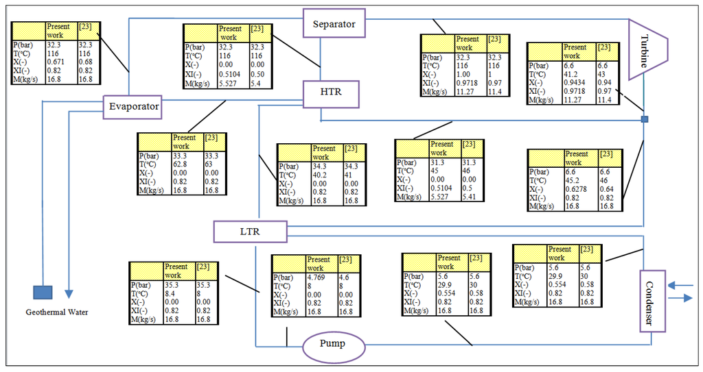
Figure 1.
Schematic diagram of the combined cycle.
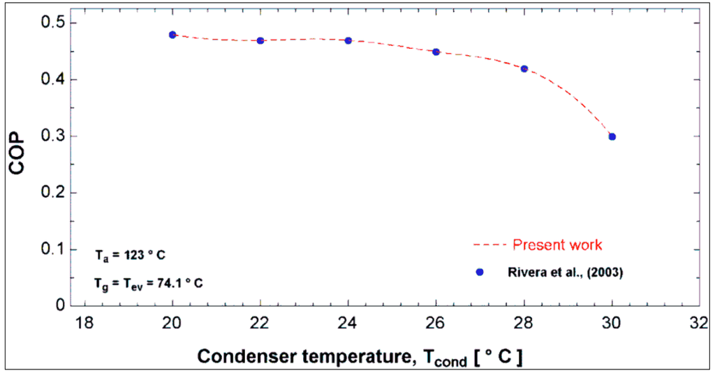
Figure 2.
(a) T-s diagram of Kalina cycle; (b) P-T diagram of the LiBr/H2O absorption heat transformer cycle.
2.2. LiBr/H2O Absorption Heat Transformer Cycle
The LiBr/H2O absorption heat transformer involves a set of processes. The saturated liquid at state 22 is subcooled in the heat exchanger, HEX, and then throttled in the expansion valve before entering the generator. Heat is added in the generator from the geothermal stream, desorbing water vapor from the lithium bromide solution. The water leaves the generator as superheated vapor, which is then condensed in the condenser before being pumped to the evaporator 2. The compressed liquid is heated in Evaporator 2 by the geothermal water and the resulting vapor passes to the absorber where it is absorbed by the solution from the HEX. The heat of absorption is used to vaporize the seawater for purification purposes. Figure 2b depicts the P-T diagram for the absorption heat transformer cycle.
2.3. Combined Cycle
The waste heat stream (states 13 to 17) is used to heat, evaporate and superheat the water (state 23). The superheated water at state 23 then combines with the concentrated lithium bromide–water solution at state 25, raising its temperature. As absorption of the vapor progresses to yield a dilute solution at state 17, heat is rejected to the stream entering at state 28, heating it to state 30, thereby providing the desired higher-grade heat output for seawater desalination. Note that in this configuration the waste heat stream is supplied in parallel rather than in series to the evaporator and generator.
3. Thermodynamic Analysis
Thermodynamic models are developed for the Kalina and LiBr/H2O cycles. In the models, each component of the system is treated as a control volume and the principle of mass conservation and the first and second laws of thermodynamics are applied to the component. Steady state operation is assumed throughout. Cycle performance is simulated by solving the corresponding equations together with the thermodynamic property relations using the EES software [30].
The mass rate balance for each component can be expressed as [31,32,33]:
∑  in = ∑ out
in = ∑ out
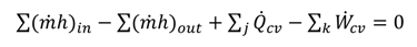
Applying the first law of thermodynamics for each component yields the following energy rate balance:
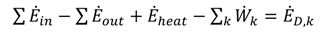
An exergy rate balance for each component of the system can be expressed as:
In addition, the absorber and mixture is subject to an ammonia mass rate balance:
∑ (x )in = ∑ (x )out
)in = ∑ (x )out
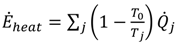
In Equations (1)–(4) the subscripts in and out denote inlet and exit states, Ẇcv is the electrical power output from the turbine less the power input to the pump,  is the total heat addition rate to the cycle from the heat source, i is the mass flow rate of the fluid, h is the specific enthalpy, ĖD is the rate of exergy destruction, and Ėheat is the net exergy transfer rate associated with heat transfer at temperature T, which is given by:
is the total heat addition rate to the cycle from the heat source, i is the mass flow rate of the fluid, h is the specific enthalpy, ĖD is the rate of exergy destruction, and Ėheat is the net exergy transfer rate associated with heat transfer at temperature T, which is given by:
In the absence of magnetic, electrical, nuclear and surface tension effects, and ignoring the kinetic and potential exergies, the total exergy rate of a stream becomes the sum of physical and chemical exergy rates [34]:
Ė = Ėph + Ėch
The first term on the right hand side of Equation (6) is calculated as [34]:
Ėph = [(h − h0) − T0 (s − s0)]
[(h − h0) − T0 (s − s0)]
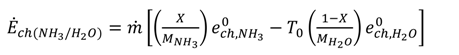
In Equation (7) the subscript 0 denotes the restricted dead state and T0 the dead state temperature. The latter term on the right hand side of Equation (6) can be evaluated for the ammonia–water mixture and LiBr/H2O as [35,36]:
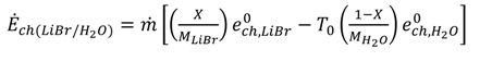
In this analysis the change in chemical exergy of LiBr is not considered. This assumption, however, introduces a small error.
A detailed exergy analysis includes calculation of exergy destructions, exergy losses, exergy efficiencies, two types of exergy destruction ratios, and exergy loss ratios for each component of the system as well as the overall system. Mathematically, all these are expressed for the kth component as follows [34]:
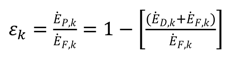
ĖD,k = ĖF,k − ĖP,k − ĖL,k
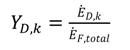
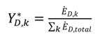
Both the Equations (12) and (13) denote the exergy destruction ratios. However, Y D compares the rate of exergy destruction in a component with the rate of total fuel exergy while  shows the ratio of component exergy destruction to the total system exergy destruction.
shows the ratio of component exergy destruction to the total system exergy destruction.Energy and exergy balances are provided in Table 1 for the components, where the flow streams are based on the states identified in Figure 1. The “Fuel-Product-Loss” (F-P-L) definitions for the system are summarized in Table 2.

Table 1.
Energy and exergy relations for the subsystems of the combined cycle.
| Subsystem | Exergy relation | Energy relation |
|---|---|---|
| Kalina cycle | ||
| Evaporator 1 | ĖD,eva 1 = T0 [ 4(s5 − s4) + 13(s14 − s13)] | 4(h5 − h4) = 13(h14 − h13) |
| Separator | ĖD,sep = T0 [ 6s6 + 8s8− 5s5] | 5x5 = 6x6 + 8x8 |
| Turbine | ĖD,Tur = T0 [ 6(s6 − s7)] | 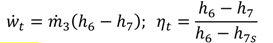 |
| LT Recuperator | ĖD,LTR = T0 [ 11(s12 − s11) + 2(s3 − s2)] | 2(h3 − h2) = 11(h12 − h11) |
| HT Recuperator | ĖD,HTR = T0 [ 3(s4 − s3) + 8(s9 − s8)] | 3(h4 − h3)= 8(h9 − h8) |
| Pump 1 | ĖD,P,1= T0 [ 1(s2 − s1)] | Wp,1 = v2(h2 − h1) |
| Condenser 1 | ĖD,con 1 = T0 [ 1(s1 − s12) + 34(s35 − s34)] |  |
| LiBr/H2O cycle | ||
| Evaporator 2 | ĖD,eva 2 = T0 [ 22(s23 − s22) + 15(s15 − s13)] | 13(h13 − h16) = 22(h22 − h23) |
| Absorber | ĖD,Abs = T0 [ 17s17 − 23s23 − 26s26 + 29(s30 − s29)] | 30(h30 − h29) =
17h17 − 23h23 − 26h26 |
| heat exchanger | ĖD,HEX = T0 [ 17(s18 − s17) + 25(s26 − s25)] | 17(h17 − h18) = 25(h25 − h26) |
| Generator | ĖD,Gen = T0 [ 20s20 − 24s24 − 19s19 + 14(s14 − s13)] | 13(h13 − h16) = 19h19 − 20h20 − 24h24 |
| Throttling valve | ĖD,V = T0 [ 24(s25 − s24)] | 18h18 = 19h19 |
| Pump 2 | ĖD,P2 = T0 [ 21(s22 − s21)] | wp,2= v21(h22 − h21) |
| Pump 3 | ĖD,P3 = T0 [ 24(s25 − s24)] | wp,3 = v24(h25 − h24) |
| Pump 4 | ĖD,P4 = T0 [ 2(8s29 − s28)] | wp,4 = v28(h29 − h28) |
| Condenser 2 | ĖD,con 2 = T0 [ 20(s21 − s20) + 35(s36 − s35)] |  |
Table 2.
“Fuel-Product-Loss” (F-P-L) definitions for the system.
| Subsystem | Fuel | Product |
|---|---|---|
| Kalina cycle | ||
| Evaporator 1 | Ė13 − Ė14 | Ė5 − Ė4 |
| Turbine | Ė6 − Ė7 | ẆTur |
| LT Recuperator | Ė11 − Ė12 | Ė3 − Ė2 |
| HT Recuperator | Ė8 − Ė9 | Ė4 − Ė3 |
| Pump 1 | Ẇp,1 | Ė2 − Ė1 |
| Condenser 1 | Ė34 − Ė35 | Ė12 − Ė1 |
| LiBr/H2O cycle | ||
| Evaporator 2 | Ė21 − Ė20 | Ė14−b −Ė16 |
| Absorber | Ė31 − Ė30 | (Ė21 + Ė27) − Ė22) |
| heat exchanger | Ė23 − Ė22 | Ė27 − Ė26 |
| Generator | Ė14 − Ė15 | Ė24 − (Ė14 + Ė18) |
| Pump 2 | Ẇp,2 | Ė20 − Ė19 |
| Pump 3 | Ẇp,3 | Ė26 − Ė25 |
| Pump 4 | Ẇp,4 | Ė30 − Ė29 |
| Condenser 2 | Ė36 − Ė37 | Ė18 − Ė19 |
3.1. Assumptions
The following assumptions are employed in this study [31]:
- (a)
- The geothermal power plants operate at a steady-state condition.
- (b)
- Pressure drops in heat exchangers and pipes are neglected.
- (c)
- The turbines and pumps have non-ideal isentropic efficiencies.
- (d)
- Kinetic and potential energy changes are negligible.
- (e)
- The geofluid is at a saturated liquid condition in the reservoir (x = 0).
- (f)
- Thermodynamic properties of pure water can be used for the geofluid.
- (g)
- Temperature and pressure losses of the geofluid are neglected in the separation and condensation processes.
3.2. Performance Evaluation
For the combined cycle, the first law efficiency is referred to as the energy utilization efficiency, which is the ratio of useful energy output to the energy input. For the combined cycle in the present study, the energy utilization efficiency can be expressed as [31]:
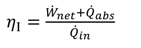 where
where
Ẇnet = ẆTur − (ẆP,1 + ẆP,2 + ẆP,3 + ẆP,4)
Similarly, the second law efficiency of the combined cycle can be expressed as:
 where
where
Ėabs = Ė31 − Ė30
Ėin = 1[(h1 − h17) − T0(s1 − s17)]
1[(h1 − h17) − T0(s1 − s17)]
3.3. Model validation
Data available in the literature are used to validate the simulation. For the case of the Kalina cycle, the numerical model was validated using previously published data [23]. Figure 3 shows the result of the validation. Similarly, Figure 4 shows the results of the validation of absorption heat transformer cycle, using data from Rivera et al. [29].
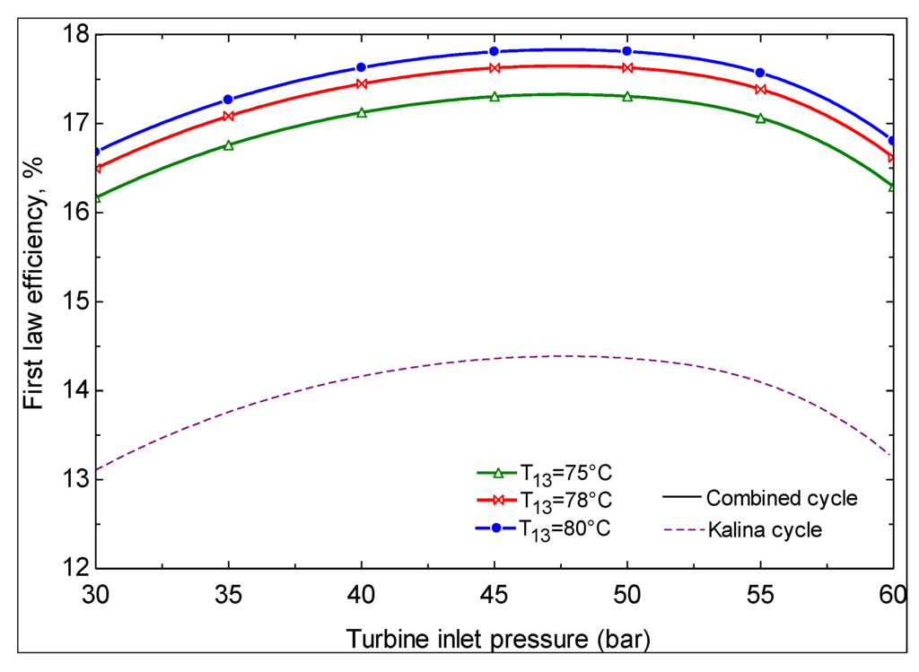
Figure 3.
Comparison of present simulation results and those from previously published work, for the thermodynamic state of the Kalina cycle.
Figure 4.
Comparison between the present simulation results and those of Rivera et al. [29] for the coefficient of performance (COP) of the absorption heat transformer system.
4. Thermoeconomic Analysis
The aim of thermoeconomic analysis is to reveal the cost-formation processes and calculate the cost per exergy unit of the product streams of the system. The unit exergetic costs of the products obtained from this procedure are used for economic optimization of the cycle. In order to calculate the unit cost of each exergy stream, a cost balance along with the required auxiliary equations are applied to each component of the cycle. For a system component receiving thermal energy and generating power, the cost-rate balance may be written as [34]:
where
and c is the unit cost of each exergy stream. The terms Ċw,k and Ċq,k are the cost rates associated with the output power from the component and input thermal energy to the component, respectively. Equation (24) states that the total cost rate of exiting exergy streams equals the total cost rate of entering exergy streams plus the total expenditure rate to accomplish the process.
∑ Ċout,k + Ċw,k = ∑ Ċin,k + Ċq,k + Żk
Ċ = cĖ
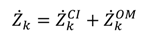
The term Żk in Equation (25) is the total cost rate associated with capital investment and operation and maintenance for the kth component:
The annual levelized capital investment for the kth component can be calculated as [34]:
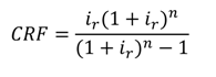
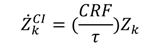 where CRF and τ are the capital recovery factor and the annual plant operation hours, respectively. The capital recovery factor is a function of the interest rate ir and the number of useful years of plant operation, n [28]:
The calculation of Zk for each component of the system is given in Appendix A. The annual levelized operation and maintenance cost for the kth component are calculated as:
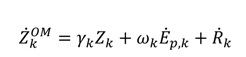 where γk and ωk account for the fixed and variable operation and maintenance costs, respectively, associated with the kth component and
  includes all the other operation and maintenance costs which are independent of investment cost and product exergy. Since the last two terms on the right side of the equation are small compared to the first, these terms may be neglected as is often done [34,35,36].
includes all the other operation and maintenance costs which are independent of investment cost and product exergy. Since the last two terms on the right side of the equation are small compared to the first, these terms may be neglected as is often done [34,35,36].The formulation of cost-rate balance and required auxiliary equations for each component of the cycle leads to the system of equations listed in Table 3.
Table 3.
Thermoeconomic relations for the subsystems of the combined cycle.
| Subsystem | Exergy relation | Subsystem | Exergy relation |
|---|---|---|---|
| Kalina cycle | LiBr/H2O cycle | ||
| Evaporator 1 | 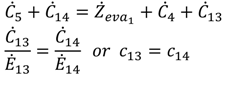 | Evaporator 2 | 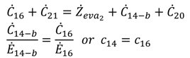 |
| Separator | 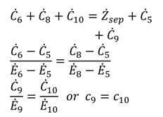 | Generator | 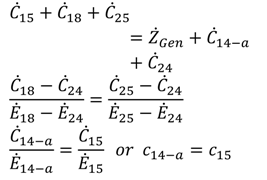 |
| Turbine | 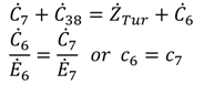 | HEX | 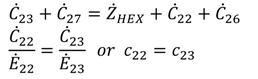 |
| LT Recuperator | 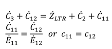 | Absorber | 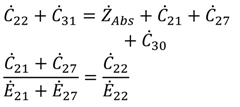 |
| HT Recuperator | 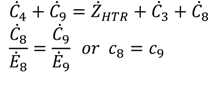 | Pump 2 | Ċ20 = ŻP,2 + Ċ19 + Ċ40 |
| Pump 1 | Ċ2 = ŻP,1 + Ċ1 + Ċ39 | Pump 3 | Ċ26 = ŻP,3 + Ċ25 + Ċ41 |
| Condenser 1 | 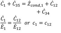 | Pump 4 | Ċ30 = ŻP,4 + Ċ29 + Ċ42 |
| Evaporator 1 | 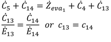 | Condenser 2 | 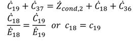 |
The linear system of equations in Table 3 includes 42 unknown variables: [x ] = {Ċ1, Ċ2, …}. The unit exergetic cost of all exergy streams of the system are obtained with the following assumptions:
- A known value is assumed for the unit exergetic cost of the geothermal source (c13 = 1.3) [37].
- The unit exergetic cost of the cooling water is neglected [29], i.e., c33 = 0, c35 = 0 and c27 = 0.
- The auxiliary equations, c14–a = c14–b = c14 and Ċ14 = Ċ14−a + Ċ14−b , are considered for streams 14–a and 14–b.
5. Results and Discussion
A parametric analysis is performed to evaluate the effects of each major parameter, namely, turbine inlet pressure (P6), evaporator exit ammonia concentration (X5) and evaporator exit water temperature (T14) on parameters related to the combined cycle performance, such as thermal and exergy efficiencies and the sum of the unit costs of the products. When one specific parameter is examined, the others are kept constant.
The basic assumptions and input parameters used in the study are given in Table 4. The performance parameters obtained from the energy and exergy analyses are shown in Table 5. For the base-case operating conditions (the conditions stated in Table 4), the thermodynamic properties and cost of streams for the combined cycle are indicated in Table 6. Finally, the cost analysis results for the combined cycle, for the base-case operating conditions, are depicted in Table 7.
Table 4.
Input data in the simulation.
| Temperature of the reference environment | 25 °C |
| Pressure of the reference environment | 1 bar |
| Temperature of water from the well | 124 °C |
| Temperature of exit water of evaporator 1 | 80 °C |
| Turbine inlet pressure | 32.3 bar |
| Temperature of water to the well | T14 − 5 |
| Temperature of solution exiting condenser | T0 + 5 |
| Temperature of generator and evaporator 2 | T16 − 3 |
| Mass flow rate of geothermal water | 89 kg/s |
| Temperature of LiBr/H2O solution | 110 °C |
| Mass flow rate of seawater | 12 kg/s |
| Ammonia mass fraction | 82% |
| Turbine isentropic efficiency | 90% |
| Pump isentropic efficiency | 80% |
Table 5.
Performance of the combined cycle.
| Turbine power (kW) | 2452 |
| Condenser 1 heat rejection rate (kW) | 14,172 |
| Pump 1 power (kW) | 80.59 |
| Pump 2 power (kW) | 0.01203 |
| Pump 3 power (kW) | 83.04 |
| Pump 4 power (kW) | 0.1108 |
| Evaporator 1 heat input rate (kW) | 16,543 |
| Evaporator 2 heat input rate (kW) | 1009 |
| Absorber heat transfer rate (kW) | 938.3 |
| Generator heat transfer rate (kW) | 857.3 |
| Condenser 2 heat rejection rate (kW) | 1011 |
| Net power output of Kalina cycle (kW) | 2371 |
| Net power output and absorber heat rate (kW) | 3226 |
| Heat input rate (kW) | 18,409 |
| Exergy input rate (kW) | 3676 |
| Thermal efficiency (%) | 17.52 |
| Exergy efficiency (%) | 67.38 |
Table 6.
Thermodynamic properties and cost of streams for the combined cycle.
| State | T (°C) | P (bar) | X | (kg/s) | Ė ph (kJ/kg) | Ė ch (kJ/kg K) | Ė (kW) | Ċ ($/h) | c ($/GJ) |
|---|---|---|---|---|---|---|---|---|---|
| 1 | 20 | 7.124 | 0 | 17.82 | 3100 | 289,132 | 292,231 | 2455 | 2.333 |
| 2 | 20.6 | 32.3 | - | 17.82 | 3164 | 289,132 | 292,295 | 2455 | 2.333 |
| 3 | 44.6 | 32.3 | - | 17.82 | 3214 | 289,132 | 292,345 | 2457 | 2.335 |
| 4 | 65.6 | 32.3 | - | 17.82 | 3382 | 289,132 | 292,513 | 2460 | 2.337 |
| 5 | 118 | 32.3 | 0.6824 | 17.82 | 6388 | 289,132 | 295,520 | 2480 | 2.331 |
| 6 | 118 | 32.3 | 1 | 12.16 | 5915 | 233,147 | 239,065 | 2007 | 2.332 |
| 7 | 46.4 | 7.124 | 0.9417 | 12.16 | 3212 | 233,147 | 236,359 | 1984 | 2.332 |
| 8 | 118 | 32.3 | 0 | 5.658 | 470.4 | 55,984 | 56,455 | 475.4 | 2.339 |
| 9 | 49.6 | 32.3 | - | 5.658 | 170.8 | 55,984 | 56,155 | 472.9 | 2.339 |
| 10 | 50 | 7.124 | - | 5.658 | 154.5 | 55,984 | 56,139 | 472.7 | 2.339 |
| 11 | 49.6 | 7.124 | 0.6382 | 17.82 | 3364 | 289,132 | 292,496 | 2457 | 2.333 |
| 12 | 40.4 | 7.124 | 0.5778 | 17.82 | 3228 | 289,132 | 292,359 | 2456 | 2.333 |
| 13 | 124 | 2.25 | - | 89 | 5085 | 0 | 5,085 | 23.8 | 1.3 |
| 14 | 80 | 2.25 | - | 89 | 1689 | 0 | 1,689 | 7.906 | 1.3 |
| 14-a | 80 | 2.25 | - | 40.89 | 913.2 | 0 | 913.2 | 4.274 | 1.3 |
| 14-b | 80 | 2.25 | - | 48.11 | 776 | 0 | 776 | 3.632 | 1.3 |
| 15 | 75 | 2.25 | - | 40.89 | 647.4 | 0 | 647.4 | 3.03 | 1.3 |
| 16 | 75 | 2.25 | - | 48.11 | 761.8 | 0 | 761.8 | 3.565 | 1.3 |
| 17 | 75 | 2.25 | - | 89 | 1409 | 0 | 1409 | 6.595 | 1.3 |
| 18 | 72 | 0.04246 | - | 0.4029 | 18.74 | 0 | 18.74 | 4.012 | 59.48 |
| 19 | 30 | 0.04246 | - | 0.4029 | 0.07032 | 0.07032 | 0.01506 | 59.48 | |
| 20 | 30 | 0.3397 | - | 0.4029 | 0.08235 | 0 | 0.08235 | 0.02232 | 75.29 |
| 21 | 72 | 0.3397 | - | 0.4029 | 134.4 | 0 | 134.4 | 1.224 | 2.529 |
| 22 | 110 | 0.3397 | 0.5511 | 5.034 | 229.5 | 5.643 | 235.2 | 5.979 | 7.063 |
| 23 | 92.73 | 0.3397 | 0.5511 | 5.034 | 193.1 | 5.643 | 198.8 | 5.055 | 7.063 |
| 24 | 64.72 | 0.04246 | 0.5511 | 5.034 | 439.2 | 5.643 | 439.2 | 11.31 | 7.063 |
| 25 | 72 | 0.04246 | 0.5982 | 4.631 | 274.1 | 4.647 | 278.8 | 8.466 | 8.437 |
| 26 | 81.27 | 0.3397 | 0.5982 | 4.631 | 286.8 | 4.647 | 291.5 | 9.307 | 8.87 |
| 27 | 101.4 | 0.3397 | 0.5982 | 4.631 | 319.7 | 4.647 | 324.3 | 10.44 | 8.942 |
| 28 | 25 | 1 | - | 0.365 | 0.03545 | 0 | 0.03545 | 0 | 0 |
| 29 | 98.19 | 0.9494 | - | 15 | 488.1 | 0 | 488.1 | 20.4 | 11.61 |
| 30 | 98.19 | 1.013 | - | 15 | 488.3 | 0 | 488.3 | 20.41 | 11.61 |
| 31 | 100 | 1.013 | - | 15 | 676.6 | 0 | 676.6 | 27.19 | 11.15 |
| 32 | 100 | 1.013 | - | 14.67 | 498.6 | 0 | 498.6 | 20.4 | 11.36 |
| 33 | 100 | 1.013 | - | 0.365 | 178 | 0 | 178 | 8.255 | 12.82 |
| 34 | 15 | 1 | 0 | 677.5 | 485.2 | 0 | 485.2 | 0 | 0 |
| 35 | 20 | 1 | - | 677.5 | 119.6 | 0 | 119.6 | 3.28 | 7.617 |
| 36 | 15 | 1 | - | 48.33 | 34.61 | 0 | 34.61 | 0 | 0 |
| 37 | 20 | 1 | - | 48.33 | 8.532 | 0 | 8.532 | 4.246 | 138.2 |
| 38 | - | - | - | - | - | - | 2452 | 22.74 | 2.257 |
| 39 | - | - | - | - | - | - | 80.59 | 0.7473 | 2.256 |
| 40 | - | - | - | - | - | - | 0.01203 | 0.00011 | 2.576 |
| 41 | - | - | - | - | - | - | 83.04 | 0.7701 | 2.576 |
| 42 | - | - | - | - | - | - | 0.1108 | 0.00102 | 2.576 |
Table 7.
Cost analysis results for combined cycle.
| Subsystem | Ė F ,k (kw) | Ė P ,k (kw) | Ė D ,k (kw) | Z ($) | Ż ($ h−1) | Y D ,k (%) |  | ε k (%) |
|---|---|---|---|---|---|---|---|---|
| Kalina cycle | ||||||||
| Evaporator 1 | 3396 | 3007 | 389 | 94,124 | 2.752 | 4.71 | 24.46 | 88.54 |
| Turbine | 2706 | 2452 | 254 | 494.9 | 0.01447 | 3.06 | 15.97 | 90.61 |
| LTR | 137 | 50 | 87 | 21,735 | 0.6354 | 1.04 | 5.47 | 36.49 |
| HTR | 300 | 168 | 132 | 14,015 | 0.4097 | 1.59 | 0.1 | 56 |
| Separator and valve | 316 | 300 | 16 | 47,663 | 1.393 | 0.19 | 1.006 | 94.93 |
| Pump 1 | 80.59 | 64 | 16.59 | 1806 | 0.05281 | 0.19 | 1.04 | 79.41 |
| Condenser 1 | 364.6 | 128 | 236.6 | 56,327 | 1.647 | 2.85 | 14.88 | 35.1 |
| LiBr/H2O cycle | ||||||||
| Evaporator 2 | 134.31 | 14.2 | 118.31 | 12,594 | 0.3682 | 1.42 | 7.44 | 10.57 |
| Absorber | 223.5 | 188.5 | 35 | 27,998 | 0.8185 | 0.42 | 2.20 | 84.34 |
| HEX | 36.4 | 32.8 | 3.6 | 5327 | 0.1557 | 0.04 | 0.22 | 90.1 |
| Generator | 492.74 | 265.8 | 226.94 | 14,434 | 0.422 | 2.73 | 14.27 | 53.94 |
| Pump 2 | 0.01204 | 0.01203 | 0.0001 | 182.8 | 0.05322 | - | - | - |
| Pump 3 | 83.04 | 12.7 | 70.34 | 1821 | 0.005345 | 0.84 | 4.42 | 15.3 |
| Pump 4 | 0.1108 | 0.11 | 0.0008 | 325.7 | 0.009521 | - | - | - |
| Condenser 2 | 26.078 | 18.66 | 4.418 | 6,344 | 0.1855 | 0.05 | 0.27 | 71.55 |
| Overall system | 8296.4 | 6701.8 | 1589.8 | 305,191.4 | 8.922366 | 19.16 | 100 | 80.77 |
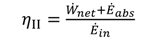
Figure 5 shows the effect of turbine inlet pressure on the first law efficiencies of the Kalina and combined cycles for various hot water temperatures exiting evaporator 1. For each temperature, an optimum pressure is observed to exist at which the first law efficiency is maximized.
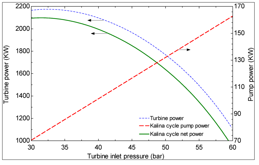
Figure 5.
Effect of turbine inlet pressure on the Kalina and combined cycle energy efficiencies for several evaporator exit temperatures.
The trend of first law efficiency in Figure 5 can be explained considering the results in Figure 6, Figure 7 and Figure 8. As Figure 6 indicates, the specific enthalpy values at the turbine inlet and exit decrease with temperature. The amounts of these reductions, however, are such that the difference between the two specific enthalpy values is maximized at a pressure of around 52 bar.
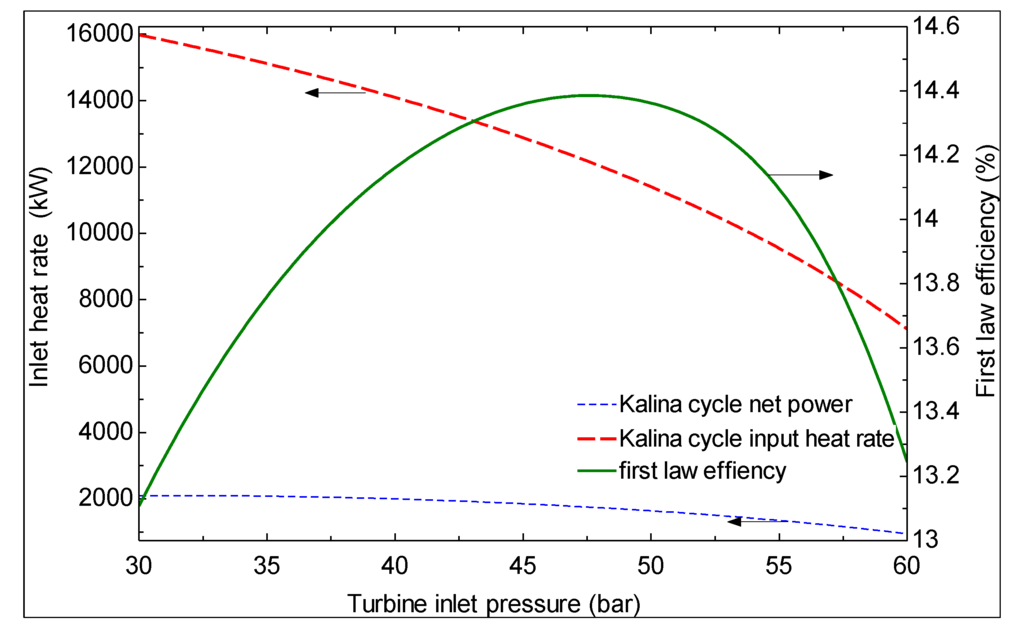
Figure 6.
Effect of turbine inlet pressure on the turbine inlet and outlet specific enthalpy values and their differences.
The results also indicate that for a known value of the evaporator 1 temperature, an increase in turbine inlet pressure causes a reduction in the turbine mass flow rate (Figure 9). Figure 7 also shows that, considering the change in pump power, the cycle net output power decreases as the turbine inlet pressure increases.
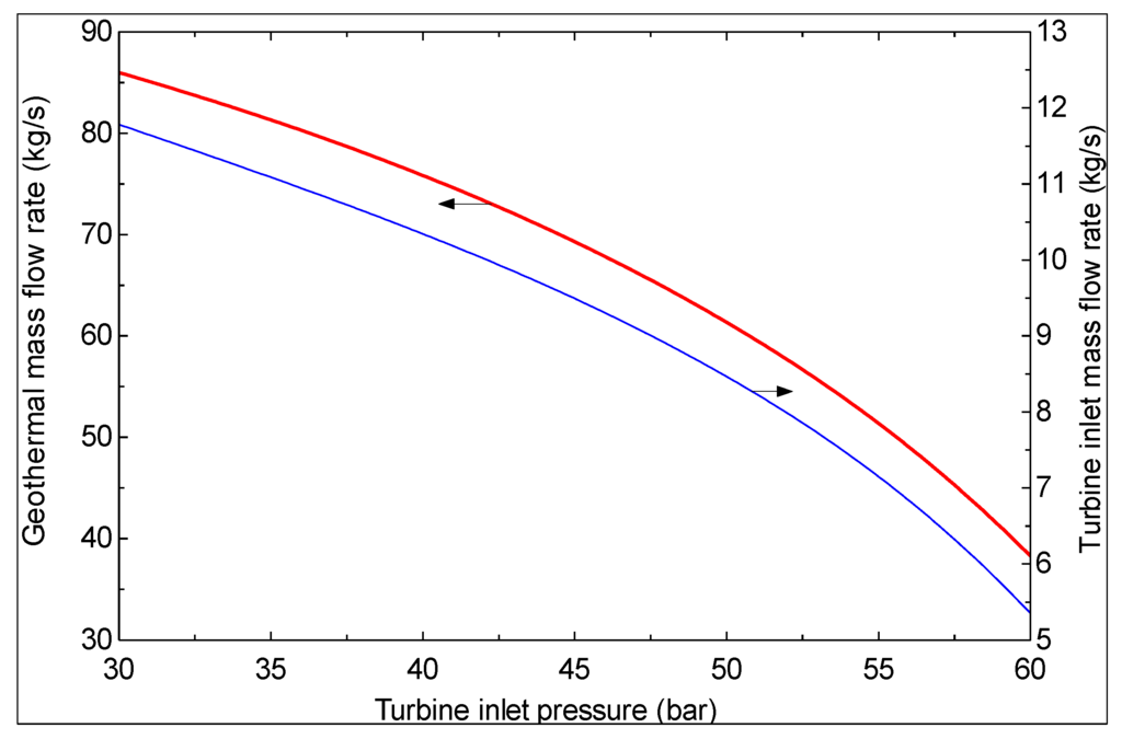
Figure 7.
Effect of turbine inlet pressure on the cycle work.
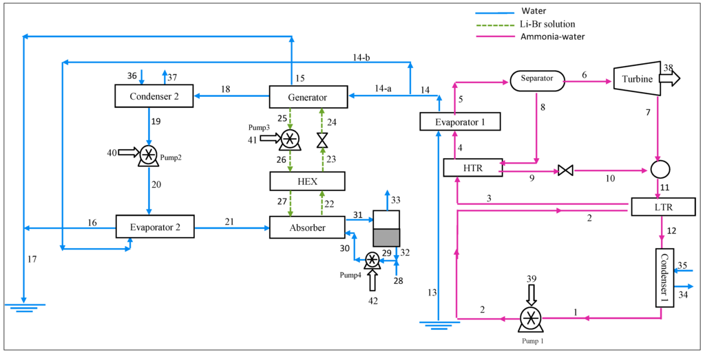
Figure 8.
Effect of turbine inlet pressure on performances of the cycles.
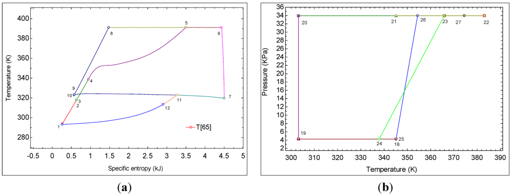
Figure 9.
Effect of turbine inlet pressure on the geothermal and turbine inlet mass flow rates.
It is observed in Figure 8 that as the turbine inlet pressure increases, the cycle input heat rate decreases. The rate of decrease in net output power, however, is such that the first law efficiency is maximized at a particular value of turbine inlet pressure.
Figure 9 shows variations in the mass flow rates of the solution passing through the turbine and the hot water, versus the turbine inlet pressure. Both the hot water and ammonia–water solution mass flow rates are seen in Figure 9 to decrease as the turbine inlet pressure increases. The first effect is due to a reduction in the cycle heat input rate and the second to the difference in ammonia concentration at the separator.
The effect of turbine inlet pressure on the second law efficiencies of the Kalina and combined cycles is shown in Figure 10 for several values of the temperature of the hot water exiting evaporator 1. It is observed that, at each temperature, there exists a pressure at which the second law efficiency is maximized. It is observed in Figure 10 that the trend of second law efficiency differs from that of the first law efficiency, particularly for the case of the Kalina cycle. It is also evident from Figure 7 that the second law efficiency is lower at higher temperatures of the hot water exiting evaporator 1. Among the combined cycle components, the highest exergy destruction (10.82% of the total) occurs in evaporator 1.
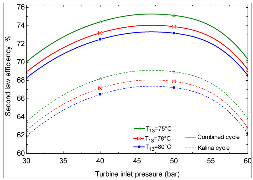
Figure 10.
Effect of turbine inlet pressure on the exergy efficiencies of the Kalina and combined cycles for several evaporator exit temperatures.
Figure 11 shows the effect of the temperature of the hot water exiting evaporator 1 on the first and second law efficiencies for a given value of turbine inlet pressure. It is observed that, as the hot water temperature increases, the first law efficiency increases and the second law efficiency decreases. The results can be explained considering the variations of the combined cycle input heat rate, input and output exergy rates and net power, as illustrated in Figure 12 and Figure 13.
The effect of turbine inlet pressure on the production rate of pure water is shown in Figure 14 for several values of the hot water temperature exiting the evaporator. It is observed that a higher turbine inlet pressure leads to a lower mass flow rate of pure water, mainly because of the lower value of the geothermal water flow rate (Figure 9). In fact the reduced geothermal water mass flow rate causes a lower lithium bromide–water mass flow rate in the absorption heat transformer cycle.
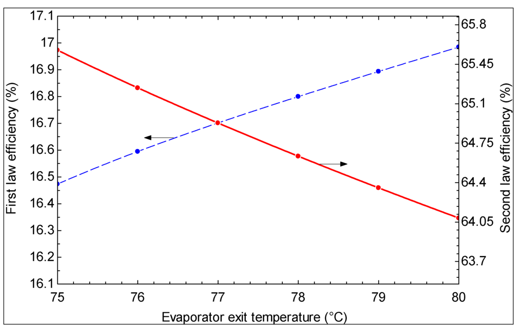
Figure 11.
Effect of evaporator exit temperature on first and second law efficiency.
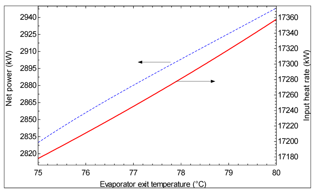
Figure 12.
Effect of evaporator exit temperature on net power and input heat rate for the combined cycle.
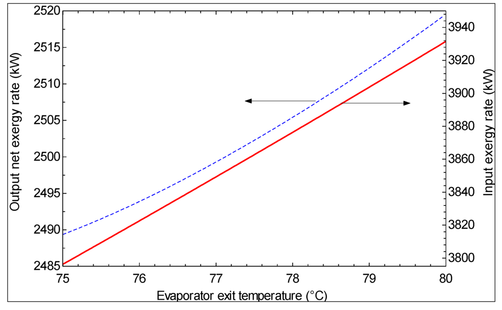
Figure 13.
Effect of evaporator exit temperature on net work rate and input heat rate for the combined cycle.
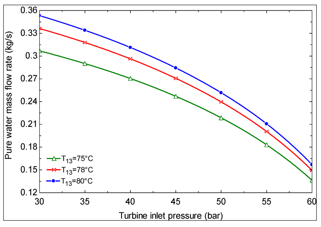
Figure 14.
Effect of turbine inlet pressure on the production rate of pure water.
Figure 15 shows the effect of turbine inlet pressure on the first law efficiency for several values of ammonia concentration. It is observed that at any ammonia concentration, an optimum pressure exists at which the first law efficiency is maximized. A comparison of Figure 9 and Figure 15 suggests it is advantageous to have a higher concentration for the solution exiting evaporator 1, because with higher concentration the efficiency rises and the required geothermal flow rate is lower.
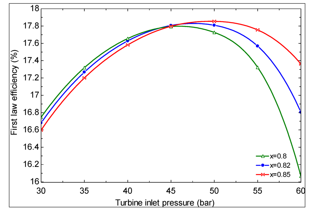
Figure 15.
Effect of turbine inlet pressure on the first law efficiency for several values of ammonia concentration.
The effect of the temperature of the hot water exiting evaporator 1 on the pure water production rate as well as the required geothermal water flow rate is depicted in Figure 16, which indicates that the pure water production rate is increased with increasing temperature due to the increase in lithium bromide-water solution mass flow rate.
The effects on the second law efficiency of the combined cycle as the geothermal water inlet temperature varies are shown in Figure 17 for several values of evaporator 1 exit temperature. From this figure, it can be inferred that low values of the geothermal water inlet temperature are not recommended and that the second law efficiency peaks at a particular value of the geothermal water inlet temperature.
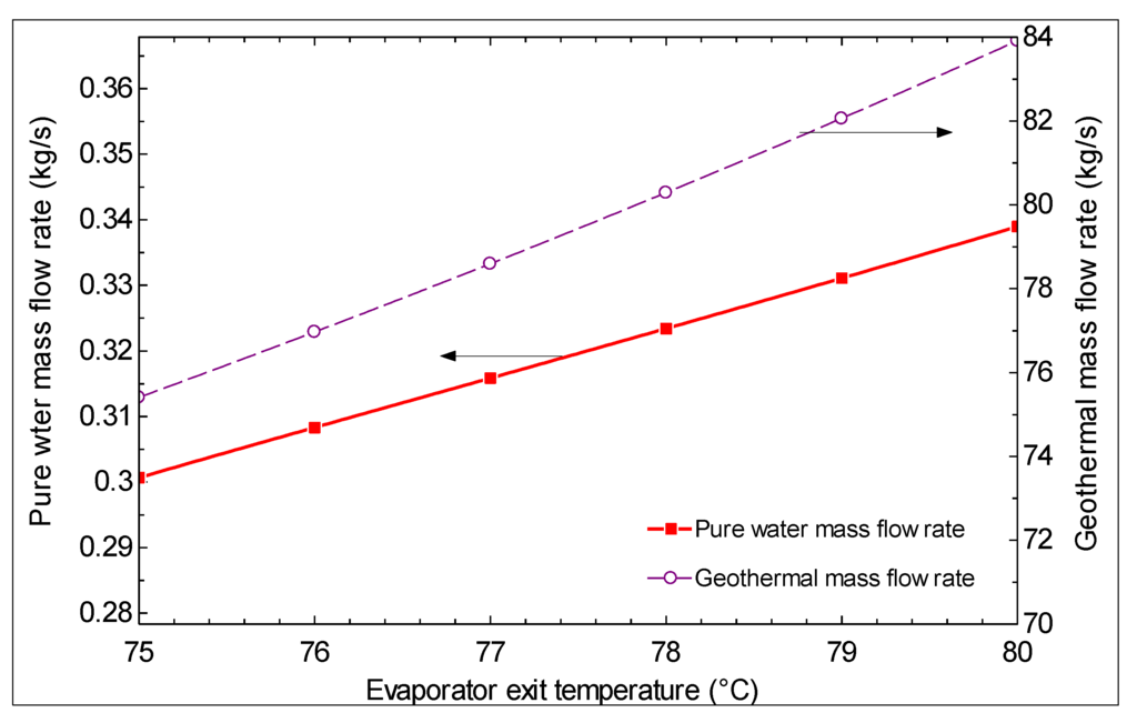
Figure 16.
Effect of temperature of hot water exiting evaporator 1 on the pure water production rate.
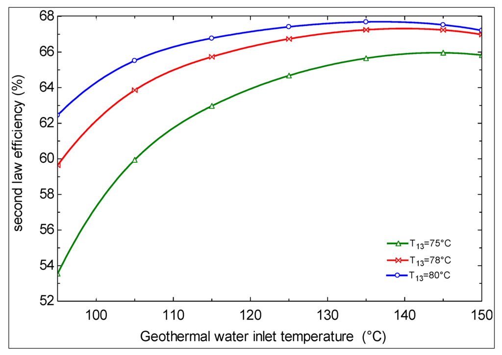
Figure 17.
Effect of geothermal water inlet temperature for several values of evaporator 1 exit temperature on second law efficiency of the combined cycle.
For purposes of comparison, it is noted that many research works are reported in the literature in which an ORC is employed for power production from geothermal energy [21,22,23]. The results of these investigations can be compared with the use of the Kalina cycle for power production from geothermal energy carried out here. Figure 18 shows the variations in first law efficiency and output power with turbine inlet pressure when either the Kalina cycle or an ORC is employed. Two different working fluids are considered for the ORC. An initial view suggests that the Kalina cycle is superior, considering both the efficiency and the output power. In Figure 18, it is seen that the first law efficiency obtained for the Kalina cycle is higher than that for the ORC by up to 25%. The higher turbine inlet pressure for the Kalina cycle, however, is a disadvantage.
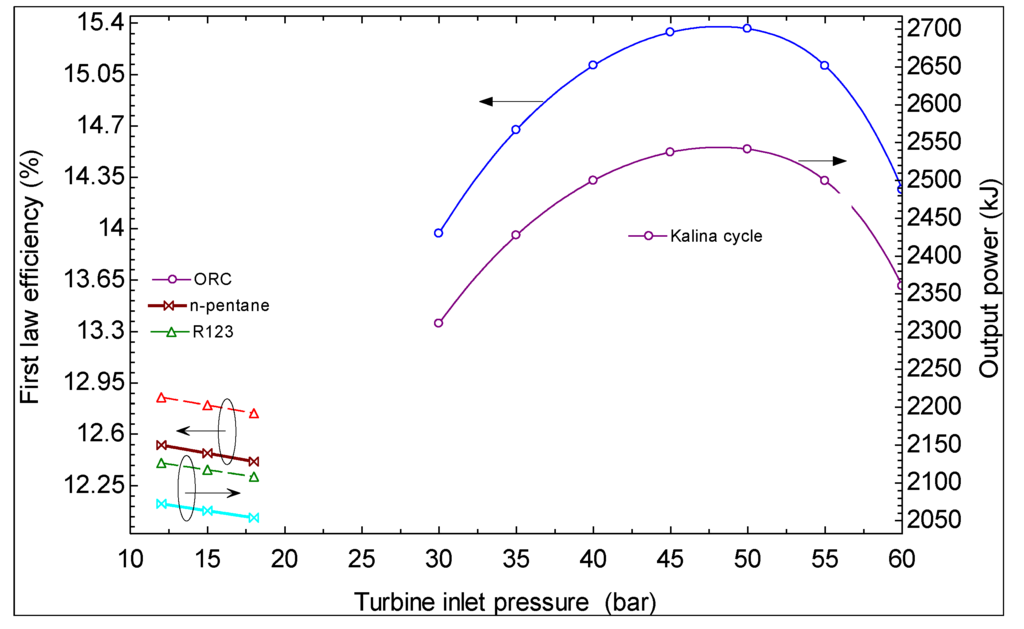
Figure 18.
Effect of turbine inlet pressure on the first law efficiency and output power of the Kalina cycle and the ORC.
6. Conclusions
The proposed cycle provide an advantageous way of utilizing geothermal energy for producing electrical power and pure water simultaneously. Specifically, the proposed cycle produces 2.94 MW of electrical power and 0.34 kg/s pure water using geothermal water with a mass flow rate of 89 kg/s at a temperature of 124 °C. Additional conclusions that can be drawn from the results follow:
- The proposed cycle, which is a combination of Kalina cycle with an ammonia–water working fluid and a heat transformer cycle with lithium bromide–water working fluid, can beneficially replace conventional geothermal power plants. The production of pure water by the proposed cycleis another advantage for the proposed cycle. The first and second law efficiencies of the proposed cycle are around 24% and 13% higher than the corresponding values for the Kalina cycle.
- The first and second law efficiencies are maximized at particular values of turbine inlet pressure. The maximum values increase with increasing ammonia concentration at the evaporator 1 outlet and increasing turbine inlet pressure.
- As the hot water temperature at the outlet of evaporator 1 increases, the first law efficiency increases and the second law efficiency decreases. However, a higher temperature is suggested for the hot water exiting evaporator 1 based on the second law efficiency, which is a more meaningful criterion.
- As the turbine inlet pressure increases and/or the hot water temperature at the exit of evaporator 1 decreases, the produced mass flow rate of pure water decreases.
- Evaporator 1 makes the highest contribution to the cycle exergy destruction, suggesting that more attention may be merited in the design of this component.
- Geothermal water temperatures of less than 124 °C are not convenient for power production with the Kalina cycle. At temperatures above this value, depending on the Kalina cycle conditions, there exists a geothermal water temperature at which the second law efficiency is maximized.
- It is found that using Kalina cycle instead of an ORC to produce power from geothermal energy is advantageous from the viewpoint of thermodynamics.
Nomenclature:
| c | Cost per exergy unit |
| Ċ | Cost rate |
| CI | Capital investment |
| CRF | Capital recovery factor |
| D | Destruction |
| Ė | Exergy rate |
| e | Specific exergy |
| Ėph | Physical exergy rate |
| Ėch | Chemical exergy rate |
 | Dead-state chemical exergy |
| h | Specific enthalpy |
| ir | Interest rate |
| M | Molecular mass |
| | Mass flow rate |
| OM | Operation and maintenance |
| P | Pressure |
 | Heat rate |
| s | Specific entropy |
| | Other operation and maintenance costs |
| T | Temperature |
| T0 | Dead-state temperature |
| v | Specific volume |
| Ẇ | Power output |
| X | Concentration |
| Z | Investment cost of components |
| Ż | Investment cost rate of components |
| τ | Annual plant operation hours |
| γk | Fixed operation and maintenance costs |
| ωk | Variable operation and maintenance costs |
Acknowledgments
Authors wish to acknowledge the financial support from University of Tabriz, Tabriz, Iran.
Author Contributions
The modeling has been carried out by Mehri Akbari for her MSc project at Tabriz University under supervision of Seyed M. S. Mahmoudi. For the manuscript, Mortaza Yari and Marc A. Rosen were advisors.
Conflicts of Interest
The authors declare no conflict of interest.
References
- Shi, X.; Che, D. A combined powesr cycle utilizing low-temperature waste heat and LNG cold energy. Energy Convers. Manag. 2009, 50, 567–575. [Google Scholar] [CrossRef]
- Vidal, A.; Best, R.; Rivero, J.; Cervantes, J. Analysis of a combined power and refrigeration cycle by the exergy method. Energy 2006, 31, 3401–3414. [Google Scholar] [CrossRef]
- Padilla, R.V.; Demirkaya, G.; Goswami, D.Y.; Stefanakos, E.; Rahman, M.M. Analysis of power and cooling cogeneration using ammonia-water mixture. Energy 2010, 35, 4649–4657. [Google Scholar] [CrossRef]
- Wang, J.; Dai, Y.; Zhang, T.; Ma, S. Parametric analysis for a new combined power and ejector-absorption refrigeration cycle. Energy 2009, 34, 1587–1593. [Google Scholar]
- Wang, J.; Dai, Y.; Gao, L. Parametric analysis and optimization for a combined power and refrigeration cycle. Appl. Energy 2008, 113, 135–146. [Google Scholar]
- Tamm, G.; Goswami, D.Y.; Lu, S.; Hasan, A.A. Theoretical and experimental investigation of an ammonia-water power and refrigeration thermodynamic cycle. Solar Energy 2004, 76, 217–228. [Google Scholar] [CrossRef]
- Zamfirescu, C.; Dincer, I. Thermodynamic analysis of a novel ammonia-water trilateral Rankine cycle. Thermochim. Acta 2008, 477, 7–15. [Google Scholar] [CrossRef]
- Maloney, J.D.; Robertson, R.C. Thermodynamic Study of Ammonia-Water Heat Power Cycles; Report CF-53-8-43; Oak Ridge National Laboratory: Oak Ridge, TN, USA, 1953. [Google Scholar]
- Ibrahim, O.M.; Kleins, S.A. Absorption power cycle. Energy 1996, 21, 21–27. [Google Scholar] [CrossRef]
- Kalina, A. Combined Cycle Waste Heat Recovery Power Systems Based on a Novel Thermodynamic Energy Cycle Utilizing Low-Temperature Heat for Power Generation. In Proceeding of the ASME Joint Power Generation Conference, Indianapolis, IN, USA, 25 September 1983; Paper 83-JPGC-GT-3. Available online: http://www.aidic.it/cet/13/35/037.pdf (accessed on 1 January 2014).
- Kalina, A. Combined cycle system with novel bottoming cycle. J. Eng. Gas Turbines Power 1984, 106, 737–742. [Google Scholar] [CrossRef]
- Kalina, A.; Leibowitz, H.M. Application of the Kalina technology to geothermal power generation. Trans. Geoth. Resour. Counc. 1989, 13, 605–611. [Google Scholar]
- El-Sayed, Y.M.; Tribus, M.A. A theoretical comparison of the Rankine and Kalina cycles. Am. Soc. Mech. Eng. 1985, 1, 97–102. Available online: http://www.uran.donetsk.ua/~masters/2006/eltf/bosov/library/kalina.pdf (accessed on 1 January 2014). [Google Scholar]
- Stecco, S.S.; Desideri, U. Thermodynamic Analysis of the Kalina Cycles: Comparisons, Problems, Perspectives. ASME Paper 89-GT-149. In Proceedings of the 34th ASME International Gas Turbine and Aeroengine Congress and Exposition, Toronto, ON, Canada, 4–8 June 1989.
- Martson, C.H. Parametric analysis of the Kalina cycle. J. Eng. Gas Turbine Power 1990, 112, 107–116. [Google Scholar] [CrossRef]
- Desideri, U.; Bidini, G. Study of possible optimization criteria for geothermal power plants. Energy Convers. Manag. 1997, 38, 1681–1691. [Google Scholar] [CrossRef]
- Dejfors, C.; Thorin, E.; Svedberg, G. Ammonia-water power cycles for direct-fired cogeneration applications. Energy Convers. Manag. 1998, 39, 1675–1681. [Google Scholar] [CrossRef]
- Jones, D.A. A Study of the Kalina Cycle System 11 for the Recovery of Industrial Waste Heat with Heat Pump Augmentation. Ph.D. Thesis, Auburn University, Auburn, Alabama, 2011. [Google Scholar]
- Madhawa, H.D.; Golubovic, M.; Worek, W.; Ikegami, Y. The performance of the Kalina cycle system (KSC-11) with low-temperature heat sources. J. Energy Resour. Technol. 2007, 129, 243–247. [Google Scholar] [CrossRef]
- Lolos, P.A.; Rogdakis, E.D. A Kalina power cycle driven by renewable energy sources. Energy 2009, 34, 457–464. [Google Scholar] [CrossRef]
- Bombarda, P.; Invernizzi, C.M.; Pietra, C. Heat recovery from diesel engine: A thermodynamic comparison between Kalina and ORC cycles. Appl. Therm. Eng. 2010, 30, 212–219. [Google Scholar] [CrossRef]
- Arslan, O. Exergoeconomic evaluation of electricity generation by the medium temperature geothermal resources, using a Kalina cycle: Simav case study. Int. J. Therm. Sci. 2010, 49, 1866–1873. [Google Scholar] [CrossRef]
- Ogriseck, S. Integration of Kalina cycle in a combined heat and power plant, a case study. Appl. Therm. Eng. 2009, 29, 2843–2848. [Google Scholar] [CrossRef]
- Sekar, S.; Saravanan, R. Experimental studies on absorption heat transformer coupled distillation system. Desalination 2011, 274, 292–301. [Google Scholar] [CrossRef]
- Rivera, W.; Siqueiros, J.; Martínez, H.; Huicochea, A. Exergy analysis of a heat transformer for water purification increasing heat source temperature. Appl. Therm. Eng. 2010, 30, 2088–2095. [Google Scholar] [CrossRef]
- Rivera, W.; Huicochea, A.; Martínez, H.; Siqueiros, J.; Juárez, D.; Cadenas, E. Exergy analysis of an experimental heat transformer for water purification. Energy 2011, 36, 320–327. [Google Scholar]
- Gomri, R. Energy and exergy analyses of seawater desalination system integrated in a solar heat transformer. Desalination 2009, 249, 188–196. [Google Scholar] [CrossRef]
- Gomri, R. Thermal seawater desalination: Possibilities of using single effect and double effect absorption heat transformer systems. Desalination 2010, 253, 112–118. [Google Scholar] [CrossRef]
- Rivera, W.; Cerezo, J.; Rivero, R.; Cervantes, J.; Best, R. Single stage and double absorption heat transformers used to recover energy in a distillation column of butane and pentane. Int. J. Energy Res. 2003, 27, 1279–1292. [Google Scholar] [CrossRef]
- Klein, S.A.; Alvarda, F.R. Engineering Equation Solver (EES); F-Chart Software: Madison, WI, USA, 2007. [Google Scholar]
- Yari, M. Exergetic analysis of various types of geothermal power plants. Renew. Energy 2010, 35, 112–121. [Google Scholar] [CrossRef]
- Nag, P.K.; Gupta, V.S.K.S. Exergy analysis of the Kalina cycle. Appl. Therm. Eng. 1998, 18, 427–439. [Google Scholar] [CrossRef]
- DiPippo, R. Second Law assessment of binary plants generating power from low-temperature geothermal fluids. Geothermics 2004, 23, 565–586. [Google Scholar] [CrossRef]
- Bejan, A.; Tsatsaronis, G.; Moran, M. Thermal Design and, Optimization; Wiley: New York, NY, USA, 1996. [Google Scholar]
- Misra, R.D.; Sahoo, P.K.; Gupta, A. Thermoeconomic evaluation and optimization of an aqua-ammonia vapour-absorption refrigeration system. Int. J. Refrig. 2006, 29, 47–59. [Google Scholar] [CrossRef]
- Rossa, J.A.; Bazzo, E. Thermodynamic modeling of an ammonia-water absorption system associated with a microturbine. Int. J. Thermodyn. 2009, 12, 38–43. [Google Scholar]
- Dorj, P. Thermoeconomic Analysis of a New Geothermal Utilization CHP Plant in Tsetserleg, Mongoloa. Master Thesis, University of Iceland, Reykjavík, Iceland, 2005. [Google Scholar]
- Misra, R.D.; Sahoo, P.K.; Sahoo, S.; Gupta, A. Thermoeconomic optimization of a single effect water/LiBr vapour absorption refrigeration system. Int. J. Refrig. 2003, 26, 158–169. [Google Scholar] [CrossRef]
- Zare, V.; Mahmoudi, S.M.S.; Yari, M.; Amidpour, M. Thermoeconomic analysis and optimization of an ammonia-water power/cooling cogeneration cycle. Energy 2012, 47, 271–283. [Google Scholar] [CrossRef]
Appendix A
For a thermoeconomic analysis, the investment costs of equipment must be evaluated. For the case of combined cycle considered in this work, the evaporator, the recuperator, the condenser, the separator, the generator, the absorber and the heat exchanger are considered as simple heat exchangers [35,38,39]. The investment costs of these components are calculated based on the weighted area using the following power law relation [34,35]:
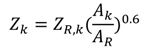 where subscript k corresponds to a heat exchanger and subscript R refers to the reference component of a particular type and size.
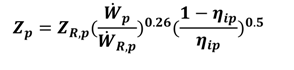
The investment cost of the pump can, respectively, be written as [35,39]:
Moreover, the investment cost of the turbine can, respectively, be written as [39]:
For each component, the reference costs for AR = 100 m2, ẆR, p = 10, in the year 2000, are given in Table A1.
Table A1.
Reference costs and overall heat transfer coefficient for each component.
| Component | Reference cost ($) [38] |
|---|---|
| Evaporator | 16,000 |
| Recuperator, heat exchanger | 12,000 |
| Separator | 16,500 |
| Condenser | 8000 |
| Generator | 17,500 |
| Absorber | 16,500 |
| pump | 2100 |
© 2014 by the authors; licensee MDPI, Basel, Switzerland. This article is an open access article distributed under the terms and conditions of the Creative Commons Attribution license (http://creativecommons.org/licenses/by/3.0/).