Experimental Investigation of Mountain Wind Fields Under Downburst Conditions

Abstract

Downbursts generate strong and transient near-surface winds that significantly influence wind flows over complex terrains. In this study, two downburst models—the impinging jet model representing the near-field region and the wall jet model representing the fully developed outflow—were experimentally investigated. The study examined the characteristics of mountain wind fields within the fully developed region, considering variations in mountain height, slope, shape, and radial position. Results show that mountain height and shape exert only minor influences on the mountain speed-up ratio, whereas slope and radial position play dominant roles: the acceleration ratio decreases with increasing radial distance and with steeper slopes. The near-surface flow is mainly affected within a vertical range of approximately 1.5 times the mountain height and a radial distance of about four times the height. By explicitly comparing the two models, this study provides the quantitative experimental relationship linking the vertical position of maximum horizontal velocity between impinging jet and wall jet flows. The comparison of mountain wind fields under equivalent positions demonstrated consistent speed-up ratios, confirming that the wall jet model can effectively reproduce the fully developed stage of downburst winds over mountainous terrain. Thus, this work offers new experimental evidence and a validated modeling framework for studying mountain wind effects under downburst conditions.

1. Introduction

Downbursts are a type of near-surface strong wind associated with severe convective weather processes such as thunderstorms. The downburst is a dense column of air (i.e., a downdraft) that generates extremely strong radial wind speeds (outflow) upon reaching the ground. These intense radial velocities typically occur at heights of 50 m above ground [1,2,3,4], posing risks to near-surface engineering structures including transmission towers, large-span roof structures, and wind turbine towers [5]. The diameter of the downdraft typically spans on the order of several kilometers, while the surrounding high-velocity outflow region generally extends to a few times the downdraft diameter [6,7,8]. Reports indicate that more than 80% of weather-related failures of power transmission lines worldwide are caused by downburst events [9].

China is also one of the regions prone to downbursts. Based on the spatiotemporal distribution characteristics of downbursts in China, such events occur frequently in the southwestern region, where mountainous terrain predominates. Consequently, the downburst wind field in these areas is significantly influenced by topographic features. Additionally, China’s power resources are unevenly distributed. The West-to-East Power Transmission initiative transports electricity concentrated in western regions to the more developed southeastern coastal areas with higher power demand. To meet the demands of large-scale, long-distance transmission and extensive resource allocation, the construction of extensive power grids inevitably traverses complex mountainous terrain. As these infrastructures are highly sensitive to wind loads [10], their design is typically governed by wind load considerations. Accurate determination of design wind loads requires a thorough understanding of wind characteristics. In mountainous topography, wind flowing over valleys or hills often experiences separation and acceleration effects [11]. More critically, complex topography and meteorological conditions in mountainous environments often generate mixed-flow wind climates. Consequently, wind speeds and its spatial distributions in mountainous regions distinctly differ from, and may even exceed, those in flat or coastal terrains. Current Chinese load codes base wind load values on conventional near-surface winds within the atmospheric boundary layer. However, downburst winds differ fundamentally from such boundary-layer winds in terms of their formation, evolution, and diffusion processes, leading to distinct wind field characteristics. Therefore, it is essential to investigate downburst wind fields under mountainous conditions and to establish corresponding downburst–mountain wind field models.

In situ field measurements represent one of the most direct and reliable approaches for investigating the wind field characteristics of downbursts, as they provide direct observations of transient near-surface flow structures. Early observational studies established the fundamental understanding of downburst generation mechanisms and wind field organization. With advances in measurement technologies, recent studies have increasingly focused on the spatiotemporal evolution of downburst winds under different terrain conditions. High-resolution observations from Doppler radar, LiDAR, and integrated monitoring systems have provided essential datasets for validating experimental and numerical studies and for improving the understanding of downburst-induced wind effects in complex environments [12,13,14].

Although field measurements can provide authentic wind field measurements, downbursts exhibit strong spatial randomness and short duration. As a result, the amount of available field data is limited, making it difficult to derive generalized patterns applicable to various scenarios without long-term monitoring. In contrast, wind tunnel testing—owing to its shorter experimental cycle and lower cost—has become one of the most widely used approaches for simulating downburst wind fields. Current wind tunnel simulation techniques for downburst wind fields worldwide primarily fall into two categories: The first aims to reproduce the entire downburst development process, such as large-scale vortex-impact jets, small-scale density-driven flows, and cold-source models. The second focus on reproducing specific downburst characteristics, including rotating plates within the atmospheric boundary layer, actively controlled multi-fan systems, and wall-mounted jet devices. However, during testing, the downburst must match the geometric scale of the building structure. Achieving this requirement with the first type of model necessitates large-scale experimental setups, which are often impractical. To overcome this limitation, researchers proposed using Type II methods to simulate the downburst’s impact on building structures without considering the full formation process of the descending jet. Among these, the impinging jet model and the wall jet model are relatively simple device with strong operability.

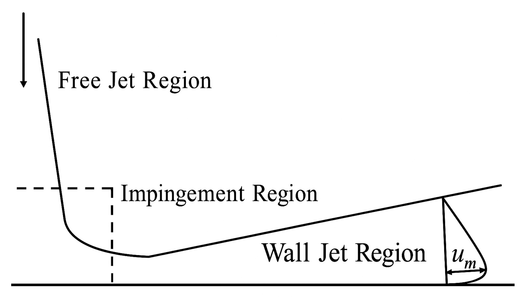
The application of the impinging jet model in downbursts was proposed by Fujita [1], which primarily relies on the interaction between the descending airflow and the ground surface. After striking the ground, the flow rapidly spreads outward. This process involves three distinct flow zones: the free jet zone, the impact development region, and the wall jet region. The free jet region, where fluid ejected from the jet nozzle enters a space with identical characteristics, generates intense downdrafts. The impact development region exhibits strong horizontal wind shear, significant pressure gradients, and noticeable variations in both wind speed and wind direction. The wall jet region can be further divided into two regions: the inner layer and the outer layer. The inner layer extends from the ground surface up to the height corresponding to the maximum wind speed and exhibits similar characteristics to a wall boundary layer, while the outer layer shares flow features comparable to those of the free jet [15].

The wall jet was first introduced by Glauert [16], who defined it as a high-velocity jet issuing parallel to a smooth wall into a semi-infinite stationary fluid of the same properties as the jet itself. After a downburst reaches its mature stage, the wall jet region becomes the dominant flow area. Wind engineering research focuses on the near-surface wind field characteristics of downbursts in this region and their response to building structures. Therefore, as long as an experime nntal setup can accurately reproduce the wind field characteristics of the wall jet region, it can be effectively used to study the impact of downbursts on buildings and other structures.

Selvam and Holmes [17] were the first to investigate the wind field downslope of a downburst. Using an impinging jet model and numerical simulation methods with a slope model of 0.25, their results showed that the wind speed at the mountaintop was lower than that at the boundary layer of the mountain. Letchford and Illidge [18] investigated the effects of radial distance and mountain slope on speed-up ratios at the summit of cosine-shaped mountains and sloped terrain using impact jet experiments and numerical simulations. Their findings indicated that the summit acceleration factor is proportional to slope gradient and inversely proportional to increasing radial distance. Mason et al. [19] investigated the mountain wind field characteristics of downbursts over slopes and bell-shaped mountains using the cold-source model. They described flow separation along the mountain surface and varied parameters such as slope, radial position, and downburst diameter to study the mountain wind field. Similarly to the mountain speed-up ratio in the impinging jet model, its value is significantly influenced by mountain slope, with the maximum acceleration effect reaching approximately 30%. Domestic researchers have also conducted similar research on mountain wind fields under downbursts. Liu Kangkang [20] investigated the mountain wind field characteristics using an impinging jet model by varying parameters such as mountain height, slope, and shape. The speed-up ratio with slope aligns with Mason’s [19] findings, while the effects of mountain height and shape are relatively minor.

In summary, previous studies have mainly examined the effects of mountain geometry on wind speed and turbulence using impinging jet experiments and numerical simulations. However, most work has focused on the speed-up ratio under idealized mountain shapes, with limited investigation into wind speed distributions at different mountain positions or the underlying acceleration mechanisms. Moreover, the flow characteristics of mountain terrain within the impinging jet model and the consistency between impinging jet and wall jet approaches have not been clearly addressed.

To fill these gaps, this study first identifies the fully developed region of a downburst-like wall jet over flat terrain, and then analyzes mountain wind fields within this region by varying key mountain parameters. The results are further compared with those obtained from the impinging jet model to establish their relationship and assess the reliability of the wall jet approach for downburst simulations. The main limitations of this study lie in the restricted range of mountain geometries considered and the simplified experimental configurations.

2. Test Overview

2.1. Experimental Investigation of Wall Jet and Impinging Jet in Wind Tunnel Tests

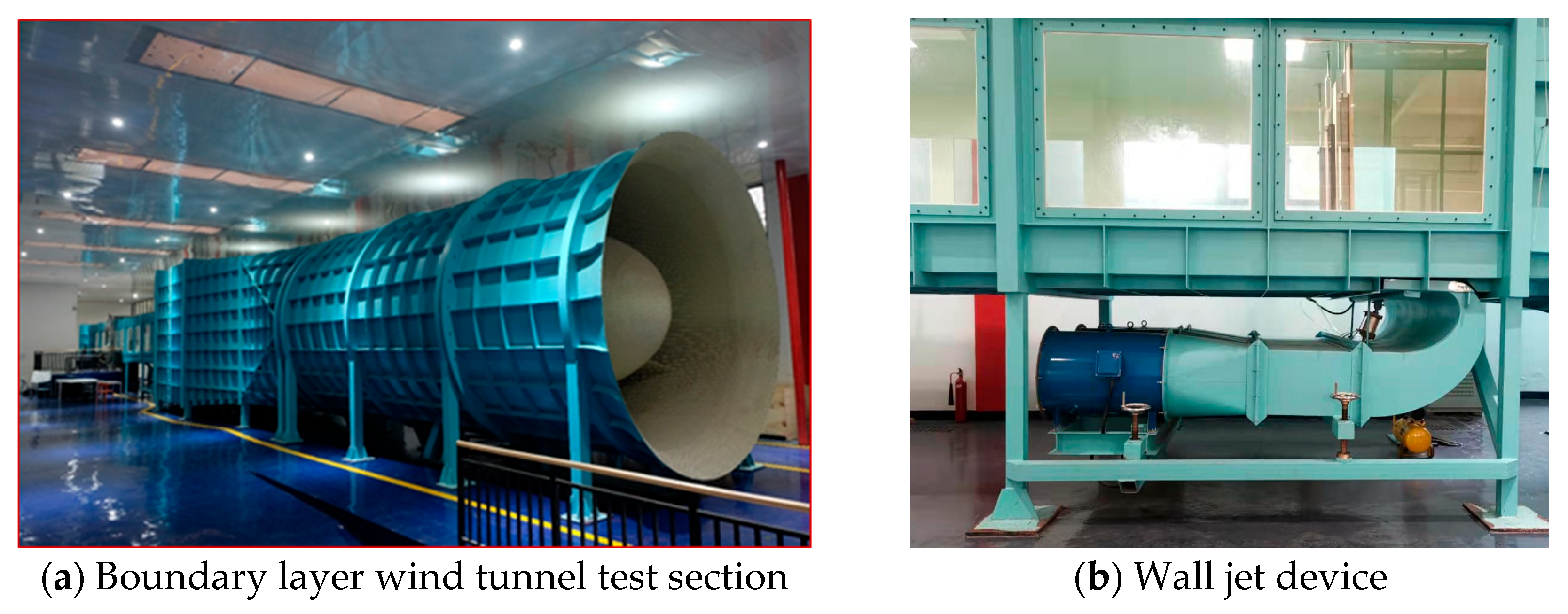
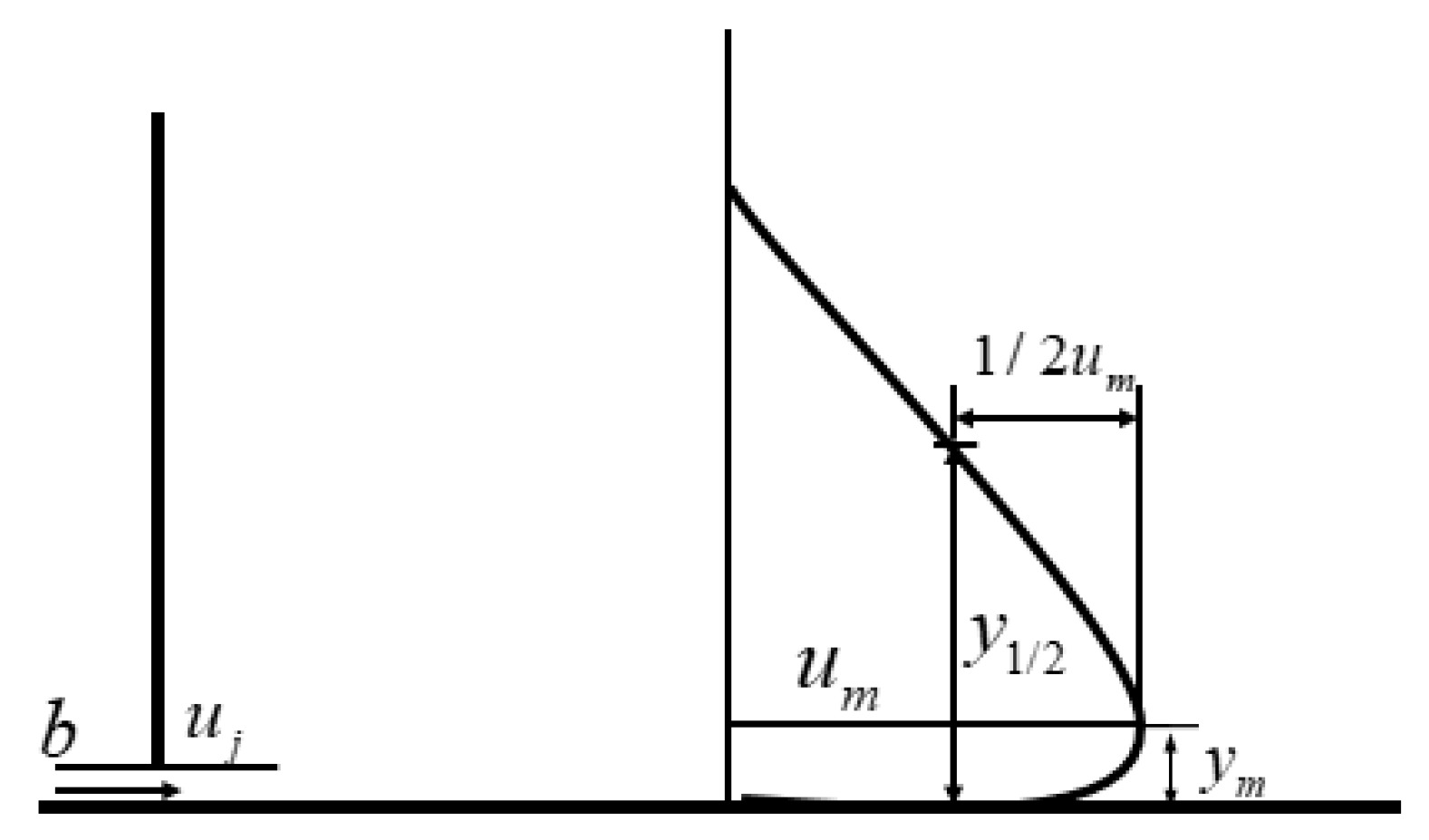
The wall jet test was conducted in the direct-flow wind tunnel laboratory at Chongqing University which is shown in Figure 1. The test section dimensions were $18 \mathrm{m}\left(L\right)\times 2.4 \mathrm{m}\left(W\right)\times 1.8 \mathrm{m}\left(H\right)$. The wall jet device was installed at the test section outlet (Figure 1b). Its outlet height was adjusted vertically using hydraulic jacks to accommodate various wind tunnel testing requirements. The wall jet model was focuses on simulating the radial development of sinking airflow to generate downburst wind profiles, as shown in Figure 2, $b$ denotes the nozzle outlet height, $u_j$ represents the jet exit velocity, $u_m$ indicates the maximum horizontal velocity at each radial position, $y_m$ corresponds to the vertical height where the maximum horizontal wind speed occurs, and $y_{1/2}$ denotes the vertical height where $1/2u_m$ is reached.

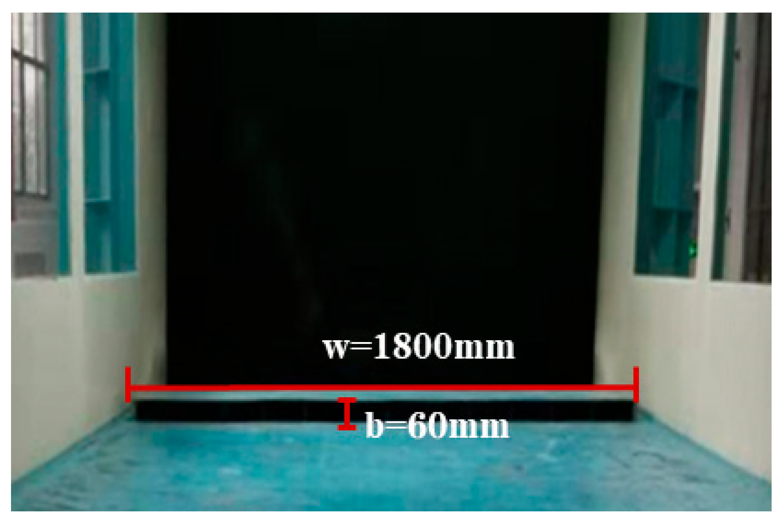
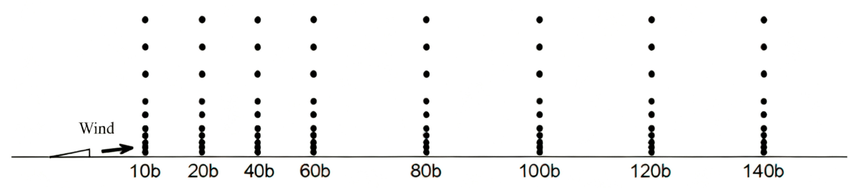
The schematic diagram of the wall jet nozzle is shown in Figure 3. The nozzle height is $b=60 \mathrm{m}\mathrm{m}$, width is $w=1800 \mathrm{m}\mathrm{m}$, and the maximum outlet air velocity can reach 45 m/s. In this experiment, an outlet air velocity of 30 m/s was adopted. Since the downdraft velocity increases with height before decreasing, vertical measurement points were arranged from dense to sparse at 10 mm, 20 mm, 30 mm, 45 mm, 60 mm, 90 mm, 120 mm, 180 mm, 240 mm, and 300 mm. To obtain a more complete steady-state wall jet flow field and the accurately location where the wall jet fully develops, measurement points were arranged at radial distances of 10b, 20b, 40b, 60b, 80b, 100b, 120b, and 140b from the nozzle position (where $\mathrm{b}$ represents the wall jet height, 60 mm). The measurement point layout is shown in Figure 4.

2.2. Introduction to Impinging Jet Wind Tunnel Tests

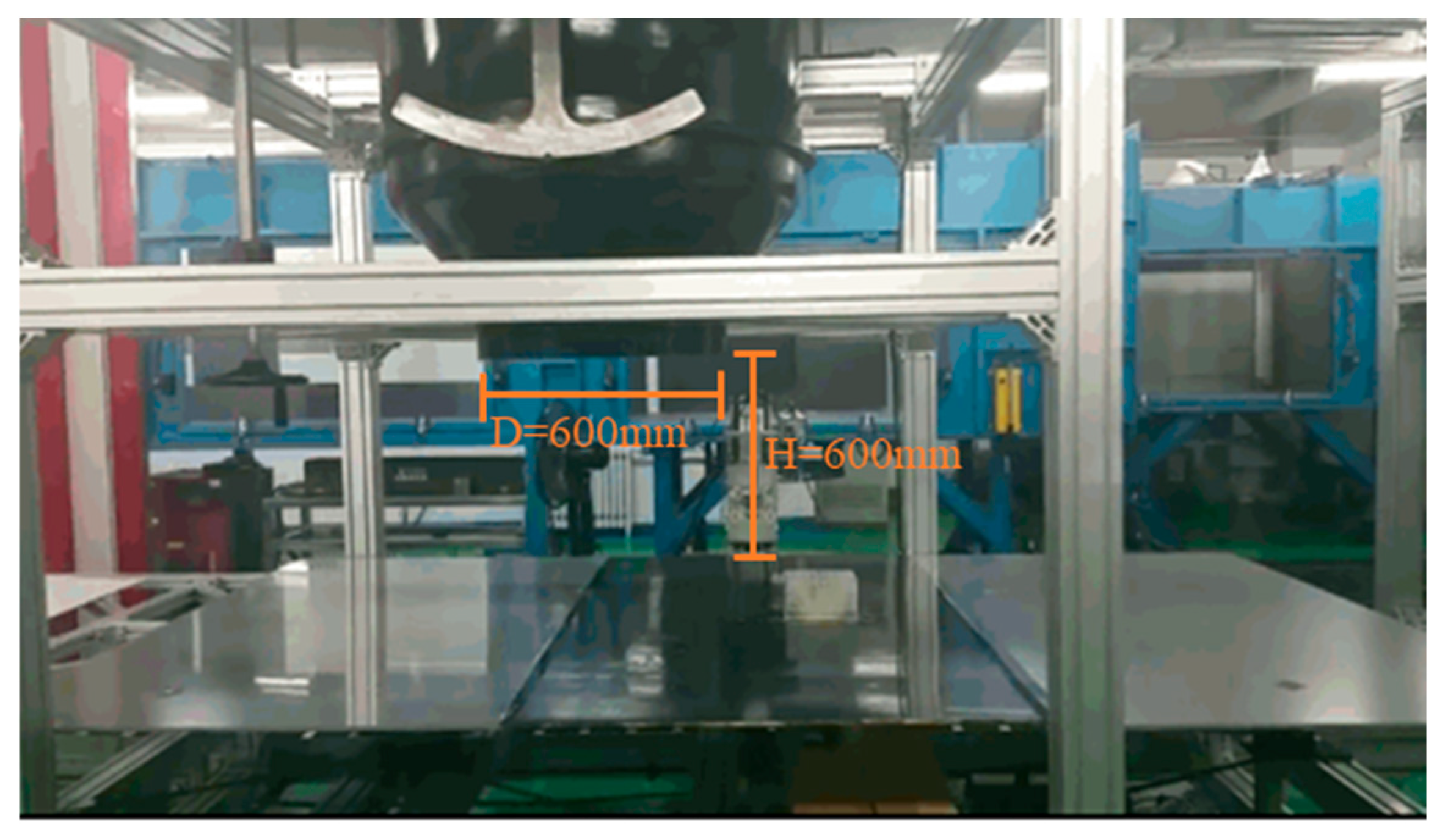
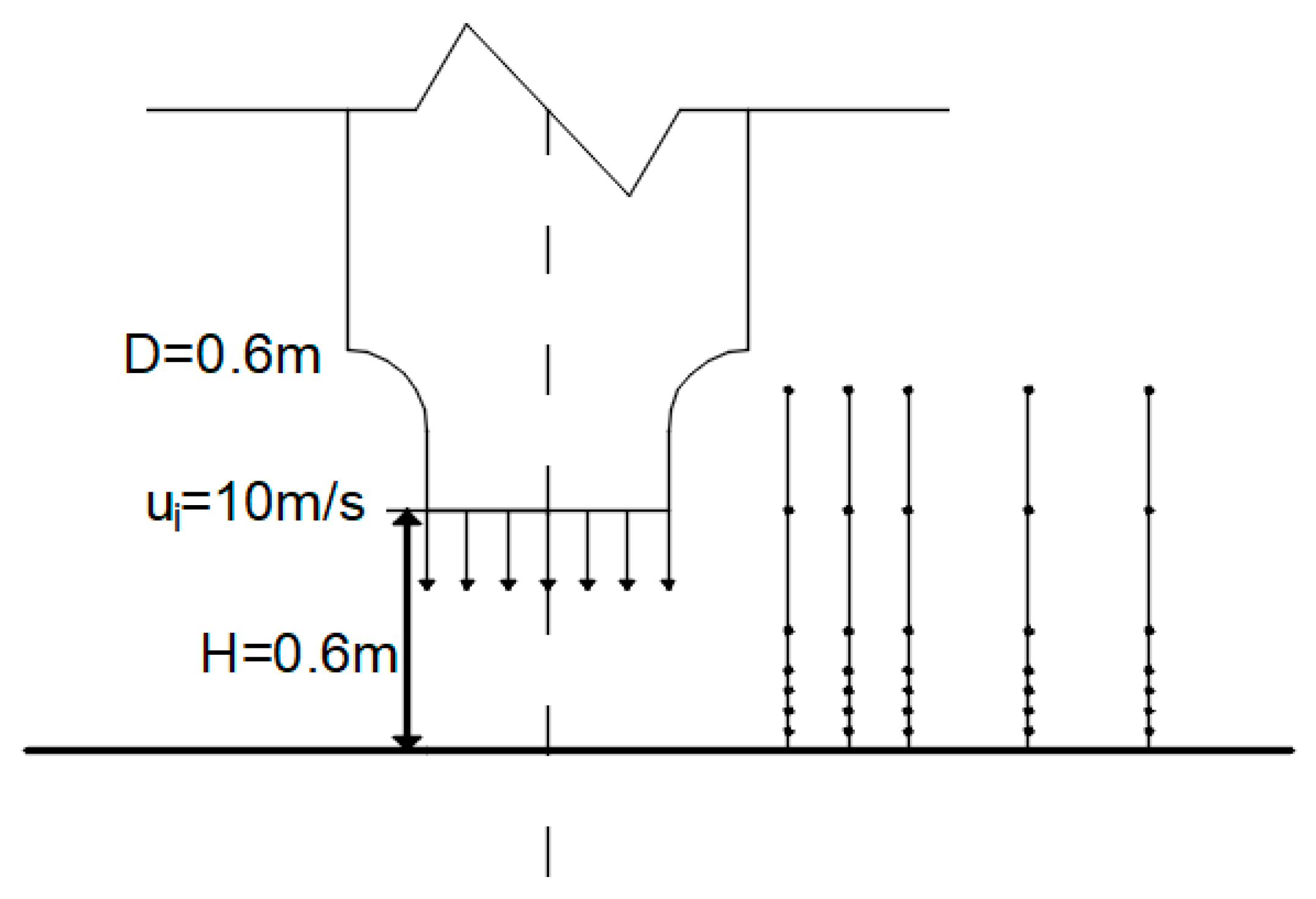
The impinging jet test was conducted at the Structural Wind Engineering and Urban Wind Environment Laboratory of Beijing Jiaotong University. As shown in Figure 5, this model simulates the sinking, impact, and radial groundward development of downbursts. The experimental setup for simulating the downburst wind field using an impinging jet device is shown in Figure 6. The downburst simulator has an outlet diameter D = 600 mm. The height between the nozzle and the floor can be adjusted via a hydraulic device within a range of 400 mm to 800 mm, with a maximum outlet wind speed of 12 m/s. In this study, the discharge height was set to H = 1.0D = 600 mm, with an outlet wind speed of 10 m/s. The measurement point layout is illustrated in Figure 7. In the impinging jet test, measurement points were arranged at radial distances of 0.5D, 0.75D, 1D, 1.5D, and 2D (D = 600 mm) from the nozzle center. Vertical measurement points were positioned at heights of 5 mm, 10 mm, 15 mm, 20 mm, 30 mm, 60 mm, and 90 mm.

2.3. Introduction to Mountain Models

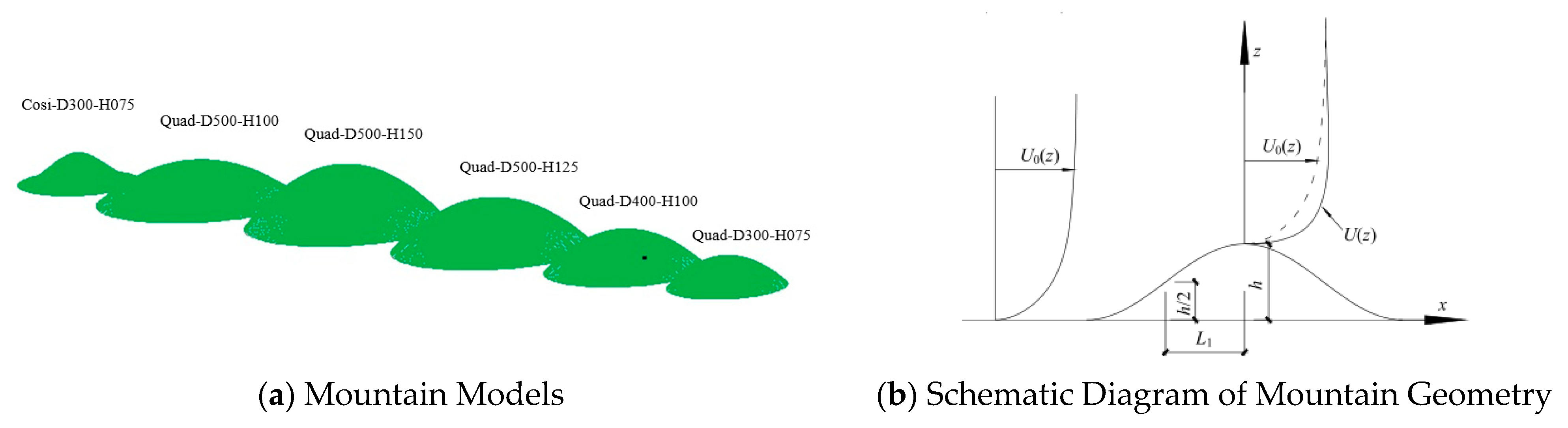
The mountain models used in this study are quadratic and cosine-shaped mountain profiles. The geometric forms of the cosine-shaped mountain and quadratic mountain models are defined by Equations (1) and (2), respectively. The mountain models used in the experiments had a geometric scale of 1:1000 and were fabricated from expanded plastic. To investigate the effects of mountain slope, height, and shape on the terrain-induced acceleration effect, the selected mountain models are listed in

Table 1. Parameters of the Experimental Mountain Model.

Mountain Model	Model Number	Mid-Mountain Angle (Angle)	Mountain Peak Angle (Angle)
Quadric D300 H075	Quad-D300-H075	0.357 (19.5°)	0.5 (26.6°)
Quadric D400 H100	Quad-D400-H100	0.357 (19.5°)	0.5 (26.6°)
Quadric D500 H125	Quad-D500-H125	0.357 (19.5°)	0.5 (26.6°)
Quadric D500 H150	Quad-D500-H150	0.43 (23.5°)	0.6 (31°)
Quadric D500 H100	Quad-D500-H100	0.285 (15.9°)	0.4 (21.8°)
Cosine Curve D300 H075	Cosi-D300-H075	0.5 (26.5°)	0.5 (26.6°)

and illustrated schematically in Figure 8a.

$$z=h{\cos }^2\left({\displaystyle \frac{\pi (x^2+y^2{)}^{\frac{1}{2}}}{4L_1}}\right)$$

(1)

$$z=h(-{\displaystyle \frac{\left(x^2+y^2\right)}{L^2}})+1$$

(2)

where $h$ represents the mountain model height; $L_1$ denotes the horizontal distance from the point at half the mountain height ($h/2$) to the peak, where $L$ is the horizontal distance from the mountain foot to the peak; $x$ and $y$ denote the distances to the mountain center. The slope angle corresponding to the mountain peak can be expressed as $\phi =h/L$, yielding the angle $\theta =\mathit{tan}\phi$. The mid-mountain angle is given by ${\phi }_s=H/2L_s$, with the corresponding angle ${\theta }_s=\mathit{tan}{\phi }_s$. Schematic diagrams of these parameters are shown in Figure 8b.

3. Downburst Wind Field Simulation

As the wall jet develops downstream, its velocity gradually decreases, and the wind profile perpendicular to the wall surface progressively expands. The maximum wind velocity $u_m$ and the half-height $y_{1/2}$ are selected to investigate the velocity decay and normal expansion of the wall jet.

3.1. Horizontal Wind Speed Profile

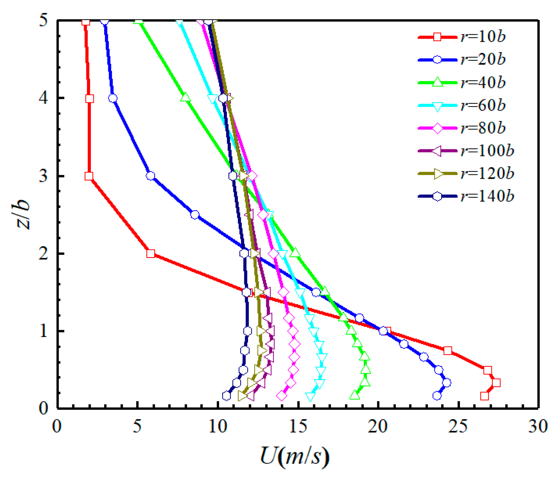
Secchi et al. [21] showed that the flow generated after jet impingement evolves into a radial wall jet developing along the surface, with self-similar behavior observed in the mean radial velocity profiles. When the velocity and turbulence intensity normalized profiles achieve self-similarity (i.e., the mean wind profiles from different experiments remain consistent after being nondimensionalized using horizontal wind speed and half-height $y_{1/2}$), the flow field characteristics become consistent. This consistency can be used to determine whether the region is fully developed. As shown in Figure 9, at $r=10\mathrm{b}$, the horizontal wind speed remains nearly constant after reaching a vertical height of 3b, and it decays rapidly between $r=10-40\mathrm{b}$. This region can be regarded as the initial development zone of the plane wall jet, representing the transition from a uniform velocity profile with low turbulence to a self-similar velocity and turbulence structure. Within this zone, the velocity gradient within the shear layer diminishes with increasing radial distance due to interactions with the wall and recirculating flow. This reduction in shear is accompanied by a gradual increase in turbulence intensity, as momentum exchange between the jet core and surrounding stagnant fluid becomes stronger. The turbulence production is primarily driven by the high shear near the jet–ambient interface and the wall, leading to enhanced mixing and a broadening of the turbulent shear layer. Shear stress at the wall induces a boundary layer configuration in the inner layer of the jet. As the boundary layer expands, the velocity within the jet core decreases. Shear forces at the interface between the jet and stagnant fluid cause additional fluid to enter the jet as it flows downstream. This leads to an increase in jet size, and the momentum transferred to the entrained fluid results in a reduction in the jet’s maximum velocity. Beyond $r>20\mathrm{b}$, the horizontal wind speed profile shape remains largely consistent, with slower velocity decay, indicating this region can be considered fully developed.

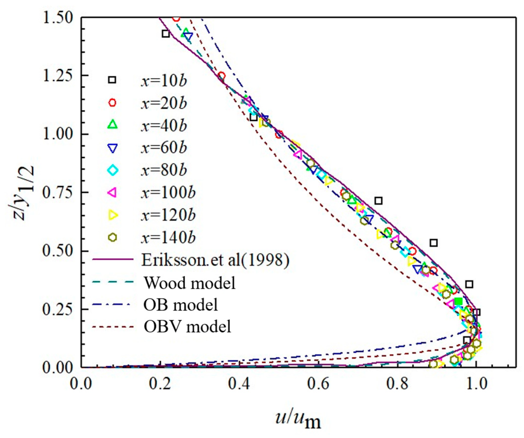
Eriksson et al. [22] employed Laser Doppler Velocimetry(LDV) for experimental measurements, which provides more precise measurement compared with other instruments. Therefore, their result at $r=70b$ were selected as a reference for comparison. Figure 10 compares the dimensionless wind profiles of horizontal wind speeds at various radial positions with the vertical wind profiles from the Wood model, OB model, OBV model, and Eriksson et al. [22] experimental data (selected at Reynolds number Re = 9600 and radial distance $r=60b$). The horizontal axis is nondimensionalized using the maximum horizontal wind speed $u_m$ at each radial position, while the vertical axis is nondimensionalized using the half-height $y_{1/2}$. The figure shows that all wind profiles pass through the same point where $u/u_m=0.5$ and $y/y_{1/2}=1$. At radial distances “$r\ge 40b$,” the dimensionless wind profiles at each radial position generally align with the Wood model and experimental results by Eriksson et al. [22], while showing larger discrepancies from the OBV model, especially below the region of maximum velocity. At the position $r=10b$, the dimensionless wind profile shows distinct differences, with a larger half-height value corresponding to the maximum wind speed. As shown in Figure 10, the region “$r\ge 20b$” represents the fully developed region, where the wind profiles demonstrate strong similarity after normalization. Conversely, the region “$r\ge 20b$” corresponds to the developing region, where noticeable deviations remain between profiles.

3.2. Characteristics of Turbulent Flow Fields

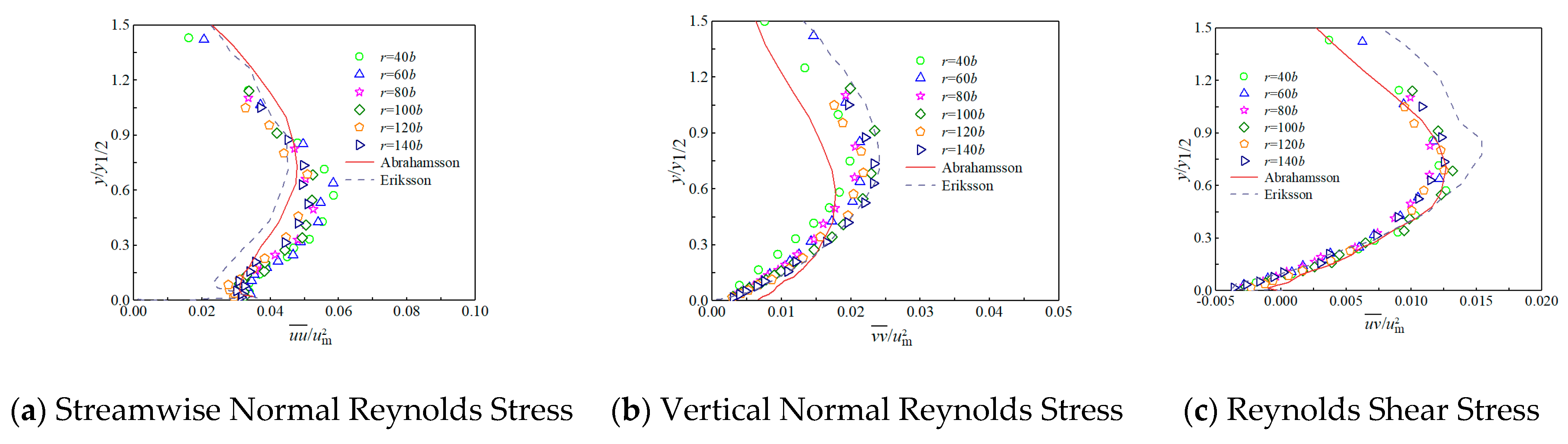
The nozzle height $b$ in the experiment is 60 mm, and the wind tunnel width is $w=1800 \mathrm{m}\mathrm{m}$, resulting in an aspect ratio of 1:30. This flow can be considered two-dimensional. For two-dimensional flow, the components of the Reynolds stress tensor are the streamwise normal stress $\overline{uu}$, the transverse normal stress $\overline{vv}$, and the Reynolds shear stress $\overline{uv}$. Eriksson et al. [22] proposed that variations in the streamwise and vertical velocity components can be experimentally determined. Therefore, the Reynolds stresses are expressed as profiles of $\overline{uu}/u_m^2$, $\overline{vv}/u_m^2$, and $\overline{uv}/u_m^2$, using the external scale $u_m^2$ for nondimensionalization. This paper analyzes Reynolds stresses in the fully developed region of the wall jet, where $r\ge 40b$. Abrahamsson et al. [23] conducted experiments using hot-wire anemometers, providing comprehensive results considered “typical” and representative. Since their inlet conditions resembled those in Eriksson [22], the results at $r=70b$ from Abrahamsson [23] and Eriksson [22] were selected for comparative analysis with the present study’s experimental data.

Figure 11a shows the streamwise normal Reynolds stress profiles. As seen in the figure, two distinct peaks appear in the wind profile: an inner peak near the wall region and an outer peak in the free shear region. The corresponding vertical coordinate range for this point is $y/y_{1/2}\approx 0.7$. The trend of turbulent intensity variation at various radial positions aligns more closely with the results reported by Abrahamsson [23]. Figure 11b shows the variation in the vertical normal Reynolds stress. With increasing height, it monotonically increases until reaching a peak corresponding to the outer shear layer. This outer peak occurs at the same position as the downstream peak, $y/y_{1/2}\approx 0.7$, with a maximum value of approximately 2.5%. The wind profile variation of $\overline{vv}/u_m^2$ more closely with Eriksson’s results than Abrahamsson’s, exhibiting a larger magnitude. Near the wall region, Eriksson’s (LDV) results are slightly higher than Abrahamsson’s (hot-wire) results. In this region, turbulence reaches approximately 20%. Due to pulse effects and wake interference, measurement errors from hot-wire calibration are unpredictable. Figure 11c shows variations in the Reynolds shear stress profile. Eriksson’s experimental results exhibit two peaks: a negative peak near the wall surface, followed by a gradual increase in Reynolds shear stress to a positive value with increasing radial distance. The present experimental results show only one peak, which may be related to the measurement method and instrumentation used. At vertical positions below $y/y_{1/2}\approx 0.5$, Eriksson’s results are slightly higher than Abrahamsson’s but generally consistent, while the experimental results agree well with Abrahamsson’s.

In summary, through analyzing the vertical wind speed profile, expansion rate, maximum velocity decay, and turbulent flow field characteristics of the wall jet over a flat surface, it can be determined that within the radial region where $r<20b$ in this experiment, the wall jet wind speed continues to develop gradually. In the radial region where $r\ge 20b$, the wind field has stabilized and is within the fully developed region of the wall jet.

4. Wall Jet Mountain Wind Field Simulation Test

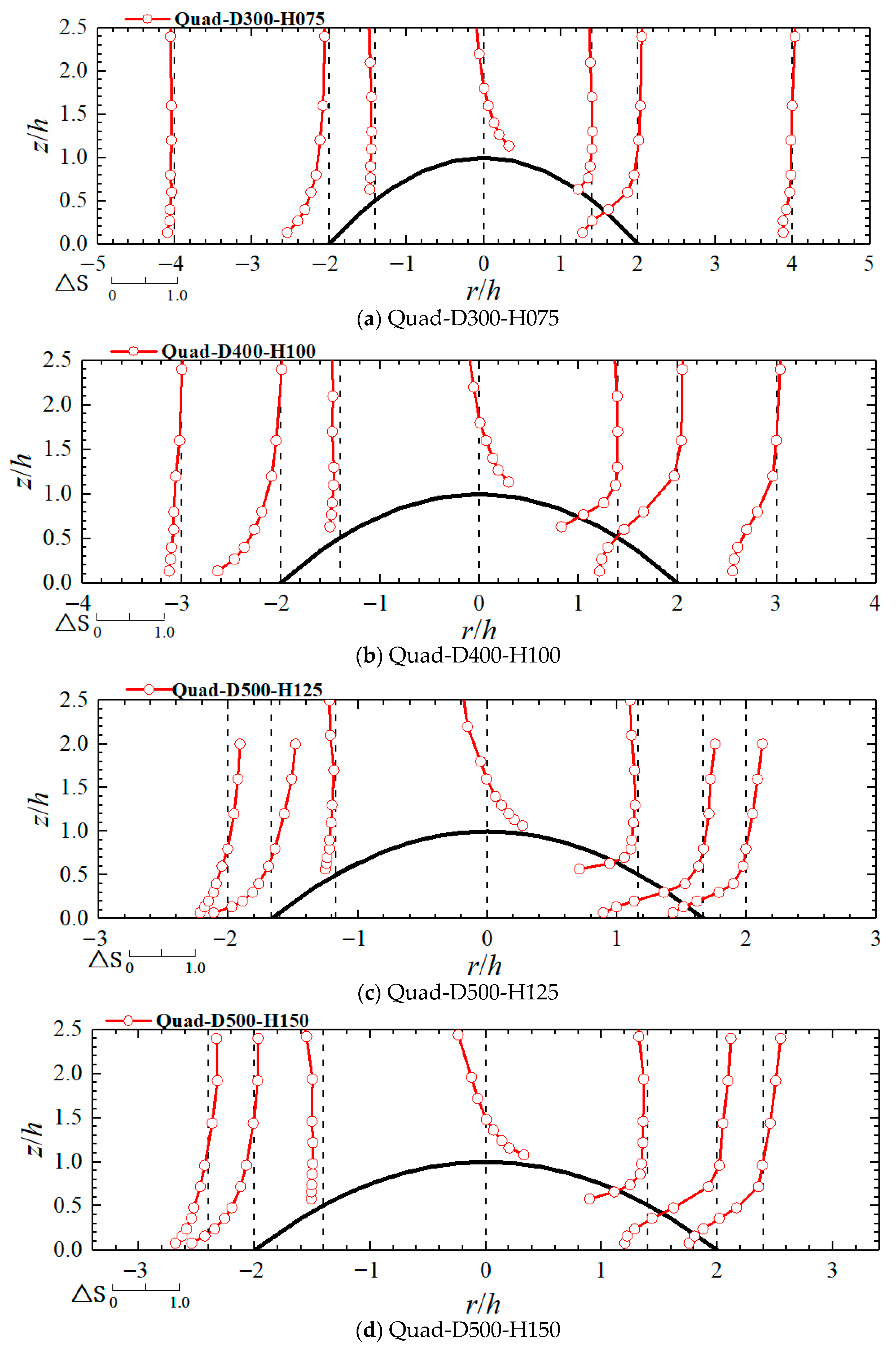
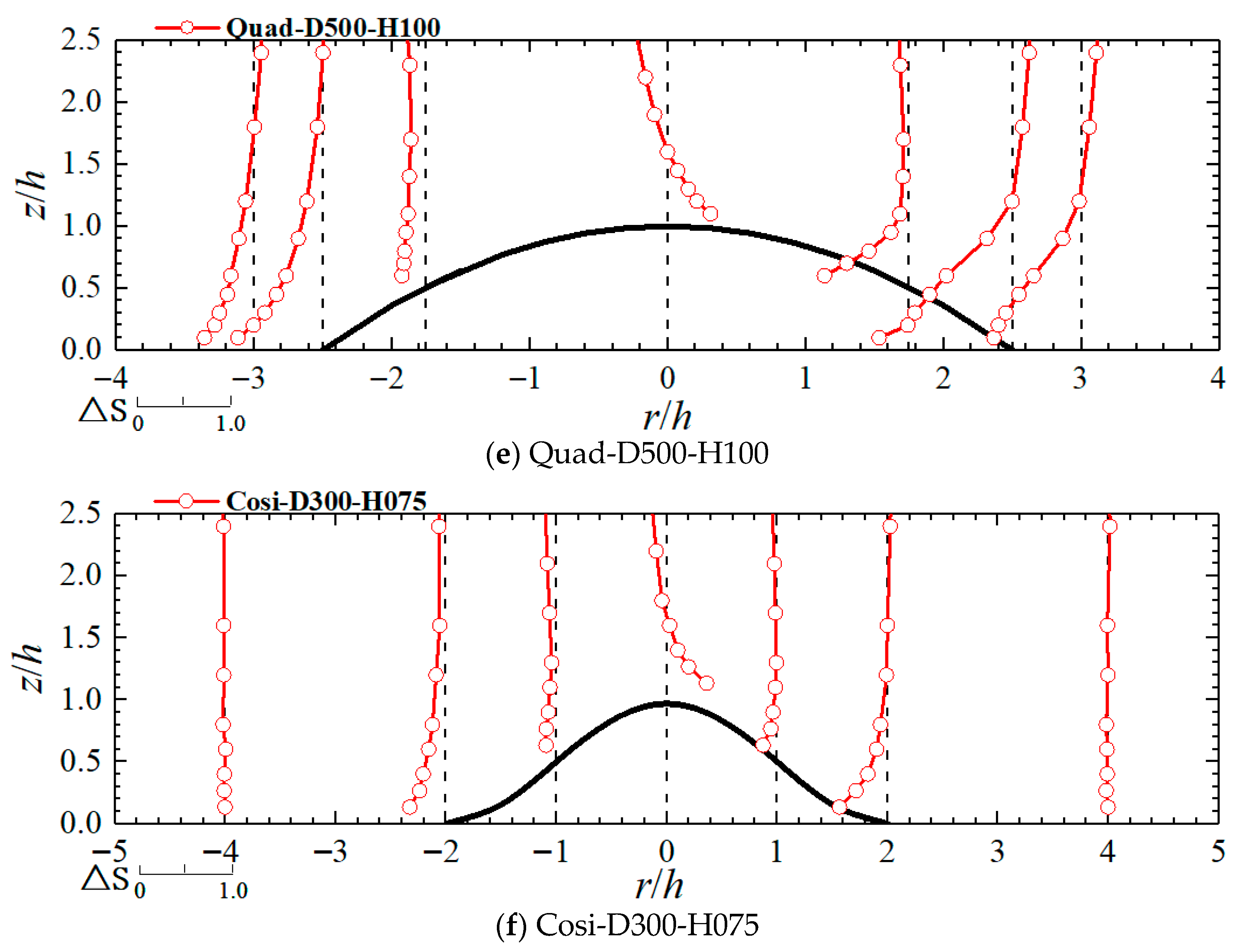
Based on the analysis of the flat-ground wind field in the previous section, a fully developed region was selected to place the mountain terrain, aiming to investigate the characteristics of the downburst mountain wind field. Additionally, the parameters of the mountain terrain model were altered to explore their impact on the mountain wind field. Figure 12 illustrates the distribution of the mountain speed-up ratio under different test conditions. The figure shows that the most pronounced acceleration occurs near the ground at the mountain peak, where the maximum speed-up ratio reaches approximately 0.33. At the peak, the speed-up ratio becomes negative with increasing height, indicating a deceleration effect in this region. The deceleration effect is most pronounced at the base of the windward and leeward foot hills, where the absolute value of the speed-up ratio can reach up to 0.9. Below a vertical height of 1.5 h, the mountain speed-up ratio increases rapidly with height; above 1.5 h, it remains essentially constant or changes minimally with height, indicating that the downdraft wind speed is no longer significantly affected by the mountain terrain. On the windward slope, the deceleration effect is insignificant and remains consistent regardless of height. On the leeward slope, near-surface deceleration occurs due to mountain obstruction. As vertical height increases, the speed-up ratio becomes positive at the same vertical position as the mountain height, and the deceleration effect essentially disappears. Therefore, when considering only acceleration effect (neglecting deceleration), the vertical height range affected by the mountain is approximately 1.5 h, which is less than the 2.5 h height range specified in the Chinese Load Code [24]. The radial position range affected by the mountain is approximately 4 h.

4.1. Effect of Mountain Height on Mountain Speed-Up Ratio

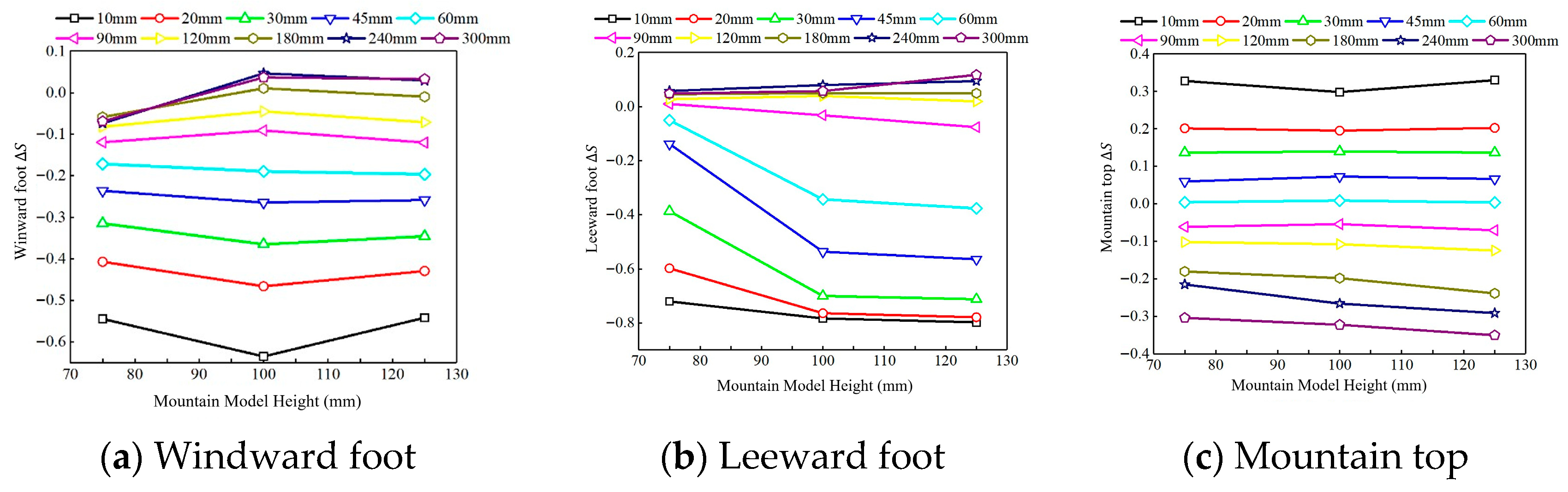
To investigate the influence of mountain height on the mountain speed-up ratio under wall jet, three cases were selected for analysis: Quad-D300-H075, Quad-D400-H100, and Quad-D500-H150, with a foot slope of 0.5. Analysis of Figure 11 and Figure 12 indicates that the influence of the mountain speed-up ratio is primarily concentrated at the mountain peak, windward foot, and the leeward foot. Therefore, the speed-up ratios at these three locations were selected for subsequent analysis. Figure 13 illustrates the speed-up ratio at different mountain heights. At the windward foot, the near-surface region is significantly affected by mountain height, exhibiting pronounced deceleration with a maximum absolute value of 0.62. The absolute value of the speed-up ratio decays most rapidly at vertical heights between 10 and 20 mm, turning positive after reaching 180 mm. At the leeward foot, the speed-up ratio reaches an absolute value of 0.8, indicating a pronounced acceleration effect. When z < 60 mm (i.e., measurement points below the mountain height), a deceleration effect occurs, with the absolute value of the speed-up ratio increasing as the mountain height increases. The higher the mountain, the larger the influence region at the leeward side. When z > 120 mm (exceeding the mountain height), the speed-up ratio at upper measurement points remains constant. As shown in Figure 13c, the maximum speed-up ratio at the mountain top can reach 0.32, and it decreases rapidly between 10 and 20 mm. At z < 60 mm, the mountain top exhibits an acceleration effect, while a deceleration effect occurs at z > 60 mm. Between 20 and 120 mm, the top speed-up ratio follows a horizontal straight line, unaffected by mountain height. At higher elevations, the speed-up ratio decreases when the mountain model is taller, possibly due to measurement inaccuracies in the Cobra probe at greater heights. Therefore, the mountain height has a minor impact on the windward and mountain top but significantly influences the deceleration effect on the leeward side. This effect is confined within the mountain’s height. When the vertical height exceeds the mountain height, the speed-up ratio remains unaffected by the mountain height.

4.2. Effect of Mountain Slope on Mountain Speed-Up Ratio

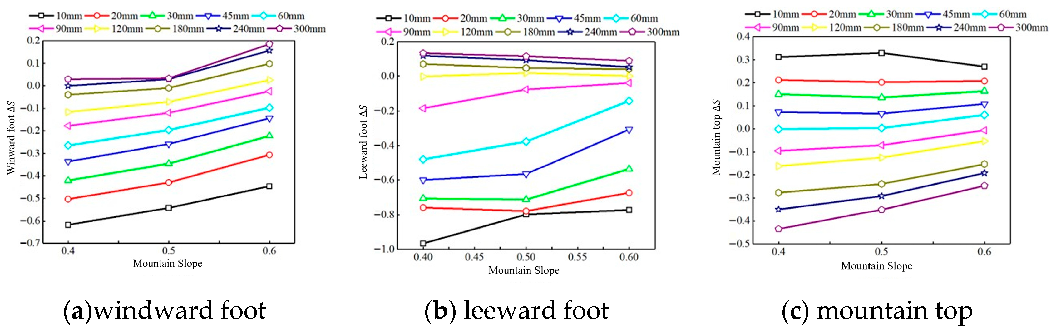
To investigate the influence of mountain slope on the speed-up ratio of wall jet in mountainous terrain, three cases—Quad-D500-H100, Quad-D500-H125, and Quad-D500-H150—were selected for analysis. The corresponding mountain top slopes were 0.4, 0.5, and 0.6, respectively.

Figure 14 illustrates the mountain speed-up ratio at the windward foot, leeward foot, and top of a mountain under varying mountain slope. As shown in Figure 14a, the windward foot region exhibits significant slope influence. With increasing mountain slope, the speed-up ratio rises accordingly. At vertical heights exceeding 180 mm, the speed-up ratio becomes positive, indicating an acceleration effect. In the near-surface zone at the leeward foot, a deceleration effect is evident. The maximum absolute value of the speed-up ratio at 1.0. Below a vertical height of 180 mm, the speed-up ratio remains negative, with its absolute value decreasing as the mountain slope increases. Above 180 mm vertical height, an acceleration effect emerges, decreasing with increasing mountain slope, as shown in Figure 14b. Figure 14c shows the speed-up ratio at the mountain top, with a maximum value of approximately 0.32. The near-surface region is less affected by slope. At vertical heights below 60 mm, an acceleration effect occurs, and the speed-up ratio at the summit remains largely consistent across different slopes. At vertical heights exceeding 60 mm, a deceleration effect emerges, with the speed-up ratio decreasing as mountain slope increases. Overall, the mountain slope has a strong impact on the speed-up ratio: both the windward and leeward feet show evident deceleration effects, and the absolute value of the speed-up ratio decreases as the slope increases.

4.3. Effect of Mountain Shape on Mountain Speed-Up Ratio

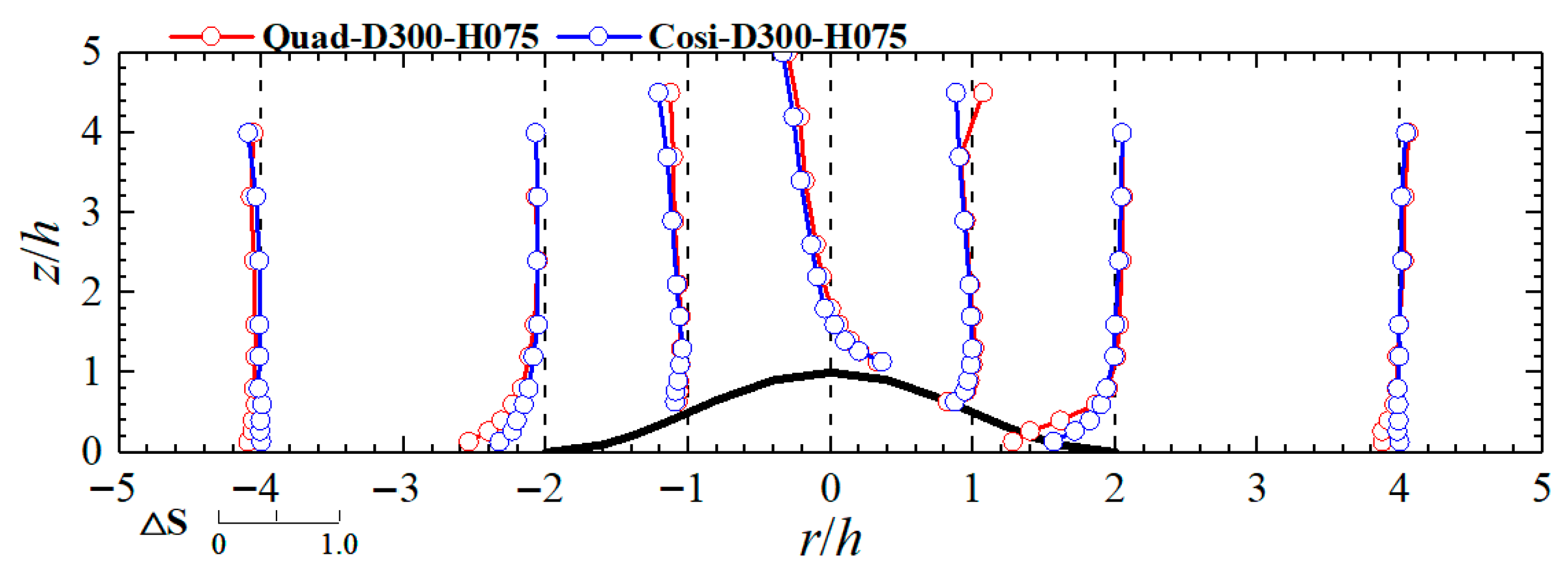
Figure 15 compares the effects of quadratic terrain (Quad-D300-H075) and cosine terrain (Cosi-D300-H075) shapes on the mountain speed-up ratio. By comparing the speed-up ratios at the windward slope, leeward slope, and mountain top, it is evident that the mountain speed-up ratios are essentially identical for both terrain models at these positions, indicating that the mountain speed-up ratio at these locations is unaffected by terrain shape. However, in the near-surface regions at the windward and leeward feet, the deceleration effect is more pronounced for the quadratic terrain model compared to the cosine terrain model.

4.4. Effect of Different Radial Distances on Mountain Speed-Up Ratio

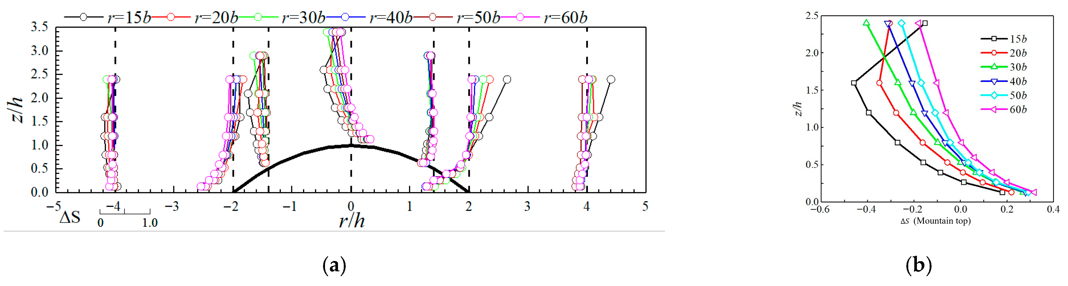
To investigate the differences in mountain speed-up ratios between the initial development and fully developed region of wall jet, mountain model Quad-D300-H075 were positioned at radial locations of 15b, 20b, 30b, 40b, 50b, and 60b. Figure 16 compares the mountain speed-up ratios at these different radial positions. As shown in Figure 16a, at radial distances of 15b and 20b, the mountain speed-up ratio exhibits a distinct trend compared to that in the fully developed region. The deceleration effect is more pronounced in the windward region. At the leeward mountain foot, 1.0h above ground level, the mountain speed-up ratio is positive and decreases with increasing radial distance. Figure 16b analyzes the speed-up ratios at different radial positions on the mountain top. As the radial distance increases, the mountain top speed-up ratio increases, though the increase is not significant within the fully developed region. At vertical heights above ground level exceeding 1.5h, the mountain top speed-up ratios at positions 15b and 20b turned positive again after deceleration. This occurred because the flat-ground wind profile had not yet fully developed in this region.

5. Comparison of Impinging Jets and Wall Jets

This section establishes the relationship between the impinging jet model and the wall jet model based on the characteristics of flat terrain wind fields. Mountain models were placed at the corresponding positions to investigate the speed-up ratios, demonstrating the effectiveness of this approach.

5.1. Flat-Ground Wind Farm Contact

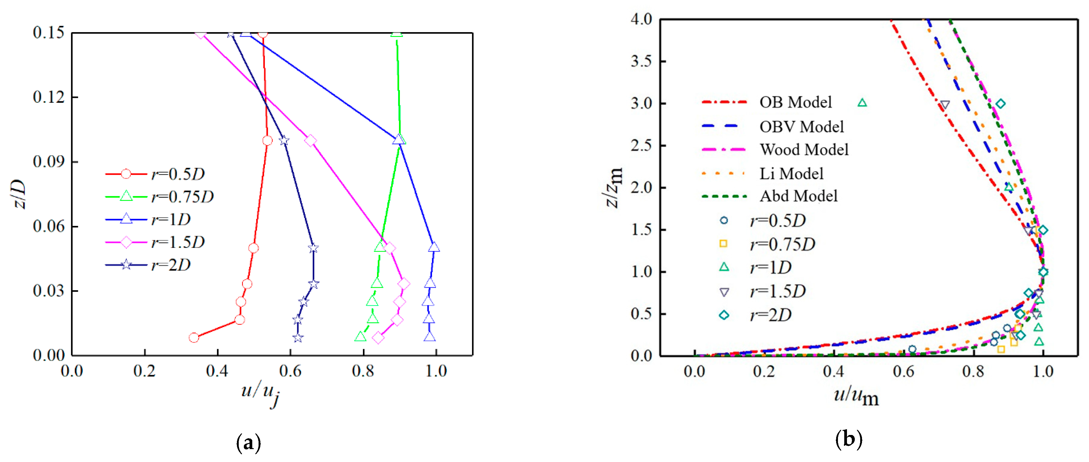
Figure 17a shows the wind profiles at various radial positions under the impinging jet model, normalized by the outflow velocity. The maximum wind speed occurs between 0.02D and 0.15D. Up to a radial position of r = 1.0D, the horizontal wind speed increases with increasing radial distance. The vertical velocity in the developing impinging region is converted into horizontal velocity, and a fully developed region has not yet formed. Figure 17b compares the dimensionless wind profiles of the impinging jet model at various radial positions with results from empirical models, normalized by maximum wind speed $u_m$ and corresponding height $y_m$. The dimensionless wind profiles at various positions for the impact jet do not fully align with the results from the Wood, Li, and Abd models. This discrepancy arises from the Kelvin-Helmholtz instability formed when the downward-moving jet interacts with the surrounding stationary air during its initial impact. This instability enables vortex rings to form, which then strike the ground, creating toroidal vortices near the surface. As these vortices expand radially outward, they detach from the ground at greater distances, subsequently generating upward wind speeds. The vertical impingement and separation of the vortex ring cause nonlinear development of the boundary layer. However, after dimensionless scaling of the shape function at each location, it is assumed that the vortex ring expands linearly along the radial distance. Beyond the radial position r = 1.0D, the dimensionless wind profile agrees well with all models, consistent with the results for fully developed regions in wall jet models.

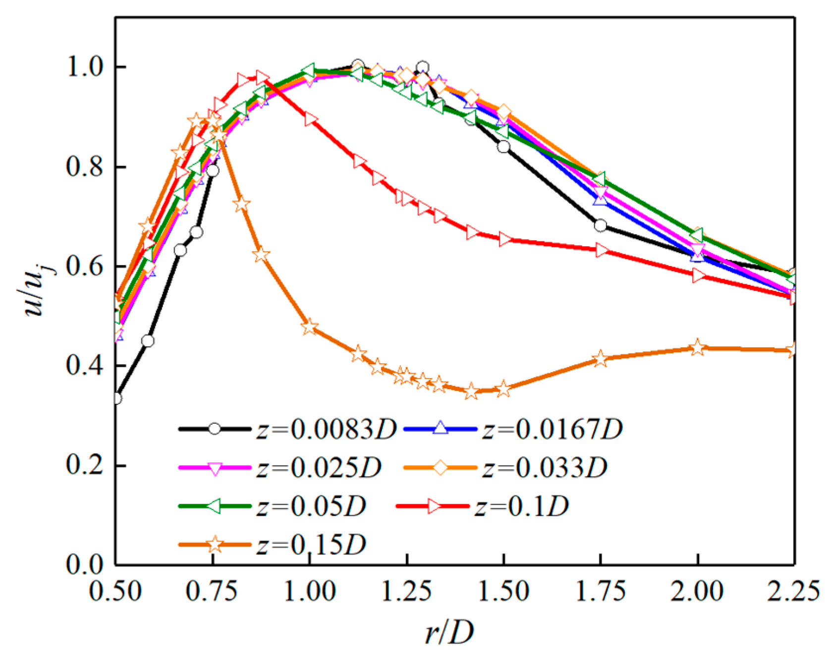
Figure 18 shows the radial wind profile of the horizontal velocity in the impinging jet model, normalized by the outlet velocity. As shown in the figure, the radial wind profile near the wall height reaches its maximum velocity at a radial distance of approximately 1.1D. The experimental results are consistent with the conclusions of Letchford et al. [18], indicating that the boundary between the developing impact region and the wall jet region in impinging jet experiments occurs between approximately 1.0D and 1.3D. In summary, the impinging jet model employed in this study can simulate the wind profile characteristics of a downburst. Furthermore, at radial positions r > 1.0D, the flow can be considered to be within the fully developed wall jet region.

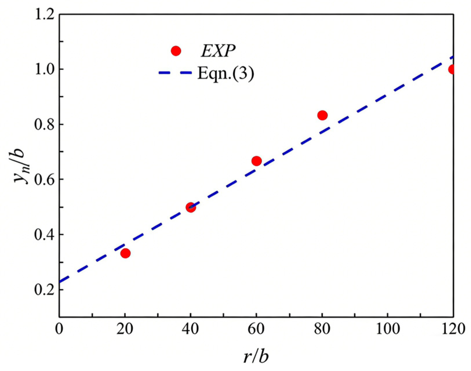
Based on the vertical wind profile results from the impinging jet model in Figure 17a,b, this study establishes the connection with the wall jet by selecting the wind profile at the radial distance $r = 1.5\mathrm{D} = 900 \mathrm{mm}$. At the radial distance r = 900 mm, the maximum wind speed corresponds to $y_m=20 \mathrm{m}\mathrm{m}$, i.e., $y_m/D=0.033$. The maximum wind speed height of the downburst primarily occurs within the range of 0.02–0.05D. Figure 19 illustrates the relationship between the height at which the maximum wind speed occurs at various radial positions and the corresponding radial position for the wall jet, as shown in Equation (3):

$${\displaystyle \frac{y_m}{b}}=0.0068\left({\displaystyle \frac{r}{b}}\right)+0.23$$

(3)

The equivalent downburst diameter of the wall jet model is determined based on the height corresponding to the maximum wind speed, as expressed in Equation (4):

$$D_{equ}={\displaystyle \frac{Y_m}{0.033}}={\displaystyle \frac{0.0068r+0.23b}{0.033}}$$

(4)

Using an impinging jet with r = 900 mm as the reference object, the equivalent radius D is calculated as $D_{equ}=\mathrm{r}=900 \mathrm{m}\mathrm{m}$. The corresponding radial position of the jet on the wall surface is calculated as r = 3380 mm = 39b.

5.2. Mountainous Wind Farm Comparison

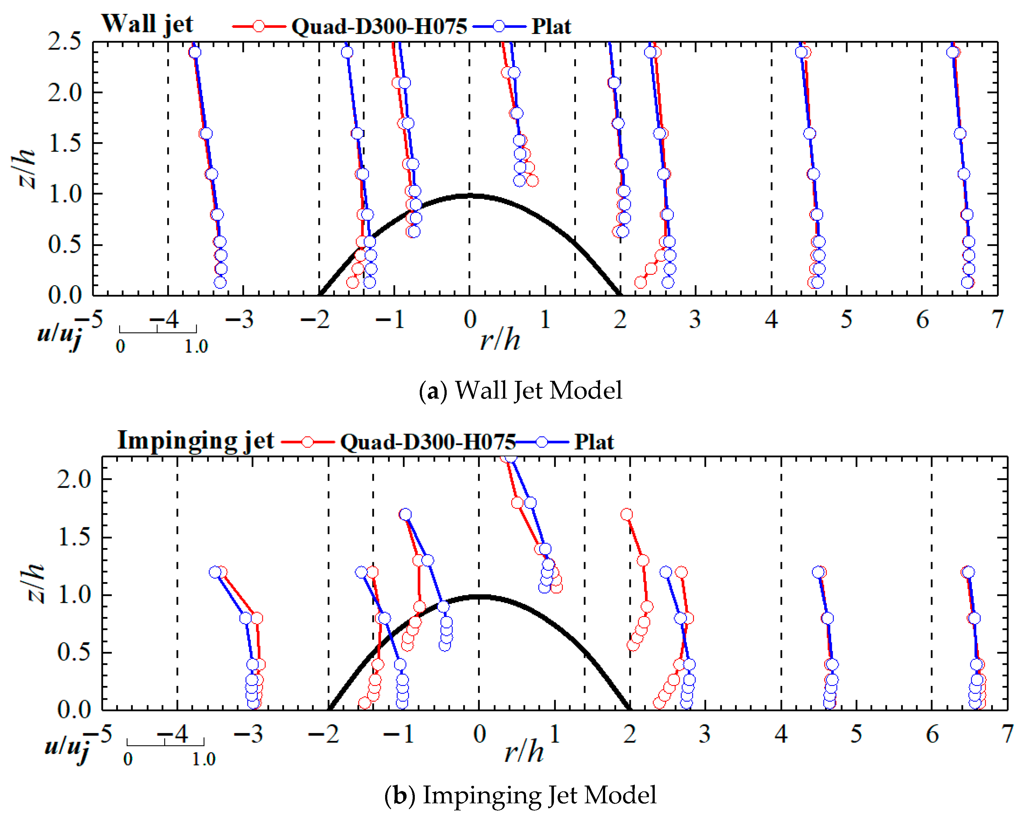
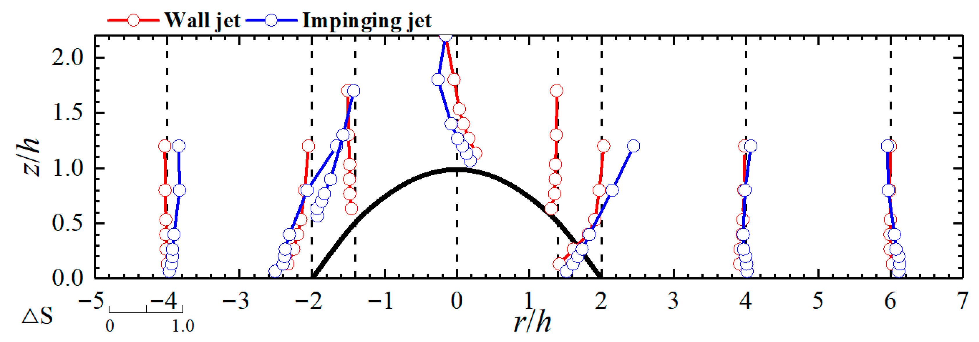
The radial positions $r=30b$ in the wall jet model and $r=1.5D$ in the impinging jet model were selected. A Quad-D300-H075 mountain was placed at these positions to compare the terrain acceleration ratios of the two models. Figure 20 compares wind speeds on slopes and flat terrain for the wall jet model and impinging jet model. The figure shows that at a radial position of 4h from the mountain center, wind speeds in both models remain unaffected by the mountain. At the windward foot of the mountain, a deceleration effect appears in both cases, which weakens with increasing height. At the mid-slope of the windward side, the wall jet model shows no significant difference between flat-ground and mountain wind speeds, while the impinging jet model exhibits a pronounced deceleration in mountain wind speeds. Similar comparisons hold for mountain wind profiles versus flat-ground profiles at the mountain summit, leeward mountain slopes, and leeward mountain foot.

Figure 21 shows the mountain speed-up ratios at corresponding locations for the impinging jet model and wall jet model. Except for the downwind foot of the mountain, the distribution trends and numerical values of the speed-up ratios are identical at all other locations. Therefore, a relationship between the wall jet and impinging jet can be established through the vertical height corresponding to their maximum horizontal velocities. Furthermore, the mountain wind field distribution is identical at the corresponding radial positions, providing a basis for directly implementing building wind effects within the fully developed region of the impinging jet within the wall jet wind field in future studies.

6. Conclusions

This study investigates the radial development of downbursts using a wall jet device and examines mountain wind field characteristics in the fully developed region. By varying mountain height, shape, slope, and radial distance, the influences of different mountain models were analyzed. A relationship between the impinging jet and wall jet models was further established based on the location of maximum wind speed and validated through comparisons of mountain speed-up ratios under both models. Compared with earlier studies that mainly used idealized terrain or numerical simulations, the present work provides experimental evidence for downburst–terrain interactions under both near-field and fully developed flow conditions.

Mountain height and shape show only minor effects on the speed-up ratio, while slope and radial position exert dominant influences. The acceleration decreases with increasing radial distance and steeper slopes. These trends are consistent with previous observations, but the present experiments quantify them specifically under downburst-like inflows.

Based on the vertical height of maximum wind speed at the 1.5D radial position in the impinging jet model, a corresponding relationship with the wall jet model was established. The speed-up ratio at equivalent positions shows good agreement, confirming that the wall jet setup effectively reproduces the fully developed stage of downburst winds.

Future work should consider transient downburst evolution, more detailed terrain roughness effects, and integration with numerical simulations or field measurements to enhance applicability to real engineering scenarios.

References

1. Fujita, T.T. The Downburst: Microburst and Macroburst; Report of Projects NIMROD and JAWS; Satellite and Mesometeorology Research Project, Dept. of the Geophysical Sciences, University of Chicago: Chicago, IL, USA, 1985. [Google Scholar]
2. He, Y.; Cai, J.; Wang, R.; He, X.; Chan, P.; Fu, J. Observation of downburst wind characteristics using the Doppler profiler and near-ground measurements. Nat. Hazards 2024, 120, 4829–4851. [Google Scholar] [CrossRef] [Scilit]
3. Zhang, S.; Guo, K.; Yang, Q.; Xu, X. Review of wind field characteristics of downbursts and wind effects on structures under their action. Buildings 2024, 14, 2653. [Google Scholar] [CrossRef] [Scilit]
4. Liu, M.; Pan, Y.; Hu, J.; Zhang, C.; Yu, X.; Xie, Z. Field measurement study of intense thunderstorm outflows characteristics based on 356 m high meteorological tower. J. Wind. Eng. Ind. Aerodyn. 2023, 242, 105590. [Google Scholar] [CrossRef] [Scilit]
5. Pryor, K.L. Downburst monitoring and prediction studies. In Field Measurements for Passive Environmental Remote Sensing; Elsevier: Amsterdam, The Netherlands, 2023; pp. 411–429. [Google Scholar]
6. Yang, L.; Fang, Z.; Ma, J.; Jiao, Y.; Wang, Z. Experimental investigation of downburst-induced wind loads on rectangular high-rise buildings: Influence of geometric features. Phys. Fluids 2025, 37, 087132. [Google Scholar] [CrossRef] [Scilit]
7. Canepa, F.; Burlando, M.; Romanic, D.; Solari, G.; Hangan, H. Experimental investigation of the near-surface flow dynamics in downburst-like impinging jets. Environ. Fluid Mech. 2022, 22, 921–954. [Google Scholar] [CrossRef] [Scilit]
8. Su, L.; Li, X.; Yan, Q.; Yao, Y.; Deng, Y.; Li, M. Experimental and numerical analysis of wind load distribution on large-span double-curved spherical shell roofs under downburst conditions: Terrain effects and radial position sensitivity. Dev. Built Environ. 2025, 24, 100767. [Google Scholar] [CrossRef] [Scilit]
9. Abd-Elaal, E.-S.; Mills, J.E.; Ma, X. A review of transmission line systems under downburst wind loads. J. Wind. Eng. Ind. Aerodyn. 2018, 179, 503–513. [Google Scholar] [CrossRef] [Scilit]
10. Li, D.; Liu, J.; Liu, B.; Fan, W.; Yang, D.; Xiao, X. Simulation Analyses on a Downburst Event That Caused a Severe Tower Toppling down Accident in Zhejiang (China). Atmosphere 2023, 14, 427. [Google Scholar] [CrossRef] [Scilit]
11. Chen, Y.; Li, Y.; Yao, J.; Shen, G.; Lou, W.; Xu, H.; Guo, Y. Experimental study of downburst wind flow over a typical three-dimensional hill. Appl. Sci. 2022, 12, 3101. [Google Scholar] [CrossRef] [Scilit]
12. Zhang, X.; Lin, Z.; Gao, C.; Han, C.; Fan, L.; Zhao, X. Evaluation and Wind Field Detection of Airborne Doppler Wind Lidar with Automatic Intelligent Processing in North China. Atmosphere 2024, 15, 536. [Google Scholar] [CrossRef] [Scilit]
13. Wang, X.; Wang, H.; He, J.; Shi, Z.; Xie, C. Automated recognition of macro downburst using Doppler weather radar. Atmosphere 2022, 13, 672. [Google Scholar] [CrossRef] [Scilit]
14. Wang, N.; Cheng, H.; Yin, C. Structural analysis of wet downburst triggered by isolated thunderstorms based on wind LiDAR. LASER Technol. 2024, 48, 643–650. [Google Scholar]
15. Dong, Z.Y. Jet Mechanics; Science Press: Singapore, 2005. [Google Scholar]
16. Glauert, M.B. The wall jet. J. Fluid Mech. Digit. Arch. 1956, 1, 625–643. [Google Scholar] [CrossRef] [Scilit]
17. Selvam, R.P.; Holmes, J. Numerical simulation of thunderstorm downdrafts. J. Wind. Eng. Ind. Aerodyn. 1992, 44, 2817–2825. [Google Scholar] [CrossRef] [Scilit]
18. Letchford, C.W.; Illidge, G.C. Turbulence and topographic effects in simulated thunderstorm downdrafts by wind tunnel jet. In Wind Engineering into the 21th Century; CRC Press: Copenhagan, Denmark, 1999; pp. 1907–1912. [Google Scholar]
19. Mason, M.; Wood, G.; Fletcher, D.F. Impinging jet simulation of stationary downburst flow over topography. Wind. Struct. 2007, 10, 437–462. [Google Scholar] [CrossRef] [Scilit]
20. Yan, B.W.; Ma, C.; Liu, K.K.; Yang, Q.; Zhou, X. Experimental and numerical simulation of topographic effects over idealized three-dimensional hills induced by downburst wind flows. In Proceedings of the Engineering Mechanics Institute Conference, Pasadena, CA, USA, 19–21 June 2019. [Google Scholar]
21. Secchi, F.; Gatti, D.; Frohnapfel, B. The wall-jet region of a turbulent jet impinging on smooth and rough plates. Flow Turbul. Combust. 2023, 110, 275–299. [Google Scholar] [CrossRef] [Scilit]
22. Eriksson, J.G.; Karlsson, R.I.; Persson, J. An experimental study of a two-dimensional plane turbulent wall jet. Exp. Fluids 1998, 25, 50–60. [Google Scholar] [CrossRef] [Scilit]
23. Abrahamsson, H.; Johansson, B.; Löfdahl, L. Turbulent plane two-dimensional wall-jet in a quiescent surrounding. Eur. J. Mech. B Fluids 1994, 13, 533–556. [Google Scholar]
24. GB 50009-2012; Ministry of Housing and Urban-Rural Development of the People’s Republic of China, Load Code for the Design of Building Structures. China Architecture & Building Press: Beijing, China, 2012.
Figure 1. Wall jet simulator at Chongqing University.
Sustainability 18 00561 g001
Figure 2. The wall jet model.
Sustainability 18 00561 g002
Figure 3. The wall jet nozzle.
Sustainability 18 00561 g003
Figure 4. Layout of measurement points in the wall jet experiment.
Sustainability 18 00561 g004
Figure 5. The impinging jet model.
Sustainability 18 00561 g005
Figure 6. Impinging jet simulator at Beijing Jiaotong University.
Sustainability 18 00561 g006
Figure 7. Layout of measurement points in the impinging jet experiment.
Sustainability 18 00561 g007
Figure 8. Mountain Models Used in the Experiment.
Sustainability 18 00561 g008
Figure 9. Vertical Wind Profiles at Different Radial Positions in the Wall Jet Model.
Sustainability 18 00561 g009
Figure 10. Nondimensional Wind Profiles at Different Radial Positions in the Wall Jet Model [22].
Sustainability 18 00561 g010
Figure 11. Reynolds Stresses.
Sustainability 18 00561 g011
Figure 12. Mountain Speed-Up Ratios for Different Terrain Models under Wall Jet Experiments.
Sustainability 18 00561 g012aSustainability 18 00561 g012b
Figure 13. Comparison of mountain speed-up ratios for different mountain heights.
Sustainability 18 00561 g013
Figure 14. Comparison of mountain speed-up ratios under different mountain slopes.
Sustainability 18 00561 g014
Figure 15. Comparison of mountain speed-up ratios under different mountain shapes.
Sustainability 18 00561 g015
Figure 16. Comparison of mountain speed-up ratios at different radial positions. (a) Speed-up ratios at various radial positions. (b) Mountain-top speed-up ratios at different radial position.
Sustainability 18 00561 g016
Figure 17. Vertical wind profiles of the impinging jet model. (a) Vertical wind profiles at different radial positions. (b) Dimensionless vertical wind profiles at different radial positions.
Sustainability 18 00561 g017
Figure 18. Radial wind profiles of the impinging jet model.
Sustainability 18 00561 g018
Figure 19. Relationship between the vertical height of the maximum wind speed and the radial position in the wall jet.
Sustainability 18 00561 g019
Figure 20. Comparison of Wind Velocity between the Wall Jet Model and the Impinging Jet Model.
Sustainability 18 00561 g020
Figure 21. Comparison of Terrain Acceleration Ratios between the Wall Jet Model and the Impinging Jet Model.
Sustainability 18 00561 g021