Investigating the Role of Urban Factors in COVID-19 Transmission During the Pre- and Post-Omicron Periods: A Case Study of South Korea

Abstract

While the literature has investigated the associations between urban environments and COVID-19 infection, most studies primarily focused on urban density factors and early outbreaks, often reporting mixed results. We examined how diverse urban factors impact COVID-19 cases across 229 administrative districts in South Korea during Pre-Omicron and Post-Omicron periods. Real-time big data (Wi-Fi, GPS, and credit card transactions) were integrated to capture dynamic mobility and economic activities. Using negative binomial regression and random forest modeling, we analyzed urban factors within the D-variable framework: density (e.g., housing density), diversity (e.g., land-use mix), design (e.g., street connectivity), and destination accessibility (e.g., cultural and community facilities). The results revealed the consistent significance of density and destination-related factors across analytic approaches and transmission phases, but specific factors of significance varied over time. Residential and population densities were more related in the early phase, while employment levels and cultural and community facilities became more relevant in the later phase. Traffic volume and local consumption appeared important, though their significance is not consistent across the models. Our findings highlight the need for adaptive urban planning strategies and public health policies that consider both static and dynamic urban factors to minimize disease risks while sustaining urban vitality and health in the evolving pandemic.

1. Introduction

The novel coronavirus known as COVID-19, which belongs to the family coronavirus, first appeared in Wuhan, China in December 2019. The virus rapidly spread worldwide and as of 10 March 2023, has resulted in 676,609,995 infections and 6,881,955 deaths [1]. Compared to prior coronavirus outbreaks, such as the Severe Acute Respiratory Syndrome (SARS) in 2003 and the Middle East respiratory syndrome (MERS) in 2015, which caused fewer than 1000 deaths, COVID-19 has caused significant shock and damage to both global and local environments. Globalization, facilitated by advanced communication and transportation systems, has allowed this infectious disease to spread quickly via international and domestic travel [2,3]. Against the proliferation of COVID-19, non-pharmaceutical policy efforts have been made over the world to minimize contact and activities through travel restrictions, social distancing, and self-isolation in addition to pharmaceutical interventions [4]. Some densely populated cities such as Shanghai, China, where more intense restrictions were needed, implemented lockdowns to contain the virus.

The unprecedented pandemic situation has challenged the promotion of building dense and connected cities as a sustainable urban planning agenda. Contemporary urban planners have adopted the so-called New Urbanism paradigm, emphasizing high-density, mixed-use, transit-oriented, and pedestrian-friendly developments. Such urban development strategies have increased access to work, learn, and play, and thus benefiting residents in environmental (e.g., air quality), social (e.g., social interaction), economic (e.g., housing price), and health aspects (e.g., physical activity) [5,6,7,8,9]. However, in the early stages of the pandemic, larger metropolitan cities with a higher concentration of people and more interconnected streets were heavily affected [10,11,12,13,14]. The pandemic thus led to discussions of the long-standing belief in the beneficial role of the built environment and empirical research to determine whether built environments magnify the risk of viral infection [15,16,17].

Along with the research question, a growing body of literature has investigated the associations between dense, connected urban environments and COVID-19 since the pandemic began in 2020, but has shown the mixed results. Some studies have found significant associations between built environments with higher population and destination densities and COVID-19 infection or mortality [18,19,20,21,22,23,24,25,26,27], while others have reported nonsignificant or even negative associations [28,29,30,31,32,33,34]. For example, Wong and Li (2020) demonstrated a significant association between county-level population density and infection cases across the U.S. during from March to May 2020 in the early stages of COVID-19 [25]. In contrast, Hamidi et al. (2020) conducted the longitudinal and multilevel analyses for urban density factors that influenced the COVID-19 infection or mortality cases per 10,000 population in 1165 metropolis counties across the U.S. [31]. They showed that higher urban density was associated with lower infection and mortality rates after controlling for the metropolitan population size and other socioeconomic and health factors. The evidence of positive associations from the literature supported the hypotheses that dense, connected environments facilitating interactions among people can be identified as a risk factor for the infection [18,23,25,35,36]. In contrast, those reporting nonsignificant or negative relationships noted that enhanced access to healthcare services and outdoor exercise facilities in dense urban areas may confer health benefits (e.g., physical activity and disease prevention), ultimately preventing or mitigating COVID-19 risk [28,30,37]. Moreover, larger cities might be better positioned to implement and enforce policy measures (e.g., mask wearing, social distancing) more effectively [15,38].

The mixed findings might also stem from differences in measurement scales and operational definitions. A recent review paper noted that the literature has used various units of analysis, such as country, county, city, and district or neighborhood levels [39]. For example, some studies analyzed the county-level variables [25,31] or the zip code level variables [35], while others measured built-environment variables within specific distance grids [18] or street blocks [26]. Previous studies have been limited to conceptualizing the built environment and providing effective guidelines to operationalize variables. While the built environment is recognized as a multifaceted factor [40], most studies have narrowly analyzed urban density as a representative measure operationalized based on population [20,22,25,32], employment or activity [20,30], residential land uses [29], or housing/building units [34,41]. Only a few recent studies have incorporated land uses and destination density, measured as the number of destinations or amenities within a district or neighborhood boundaries [24,26,42,43]. Wali and Frank [42] highlighted these measurement limitations and adopted the D-variable framework (density, design, diversity, destination accessibility), which has been widely suggested in built environment research [42]. They noted that the multiple domains representing different aspects of neighborhood environments can improve the model specification and reduce the estimated bias from the endogeneity such as omitted variable bias. However, they did not fully address the varying roles of different measures within each domain. Most studies relied on static census data, which may not reflect rapid mobility changes in high population areas. Recently, so-called big data such as Wi-Fi mobile data, GPS traffic data, and credit card transactions has been increasingly used to analyze urban dynamics, which provide real-time information on mobility, behavior, and economic activity in specific areas.

While the COVID-19 pandemic progressed through several phases characterized by the emergence of new variants, such as the highly transmissible Omicron variant, most studies focused on the early phase of COVID-19. The contribution of urban density to virus transmission was a subject of significant debate in the early outbreaks, but the density effects may evolve as the pandemic dynamics shifted over time. Previous studies using mobility data found that dynamic spread of epidemics is influenced by mobility patterns, with areas of concentrated mobility experiencing faster outbreak growth [12,44,45]. This current study integrated diverse data sources, including mobility and economic activity data, to examine the impacts of diverse urban factors on COVID-19 across different time periods, from the early outbreak to the Omicron variant, divided into Pre-Omicron and Post-Omicron phases. While machine learning techniques have been increasingly applied to urban studies, COVID-19 research has largely relied on conventional statistical analyses. While the conventional statistical approaches provide interpretable coefficients that are valuable for policymakers and urban planners, they are often limited by researchers’ variable selection typically based on statistical significance from the literature and vulnerable to collinearity among variables. A machine learning approach allows many variables to be included without specifying functional forms between variables and identifying multicollinearity issues and has shown the advantages in better predictive performance [46]. A few recent studies have applied machine learning techniques to COVID-19 data [47,48], but they did not consider a comprehensive set of urban factors. In this current study, we employ machine learning techniques alongside conventional statistical analyses to identify key urban factors related to the spread of COVID-19 and to provide deeper insight to complex relationships.

2. Methods

2.1. Study Area and COVID-19

The study area encompassed the entirety of South Korea, which covers approximately 100,363 square kilometers with a population of over 51 million. South Korea has nine provinces, which are further divided into 229 administrative units including cities (“si” in Korean), counties (“gun”), and boroughs (“gu”). This study analyzed a total of 226 cities, counties, and boroughs, excluding missing and extreme values. The average number of households per administrative unit was 48,874, with a range of 758 to 636,629. The average annual household income was approximately KRW 52 million (USD 44,000), with a range of KRW 30 million (USD 25,000) to KRW 123 million (USD 104,000) per year. The average land area per administrative unit was 141.2 square kilometers, with a range of 1.78 to 605.2 square kilometers.

Figure 1 shows the daily COVID-19 infection trends in South Korea from 2020 to 2022, along with the period covered by this study. Following the initial outbreak in January 2020, the number of daily infections remained below 1000, but gradually increased and fluctuated since August 2021. South Korea responded rapidly to the pandemic, with high public compliance to government regulation. Policy measures included drive-through testing, social distancing, restrictions on the number of people in business hours, and a mobile notification system for informing the public about infected locations and for contact tracing. The transition from social distancing to normal routines began on 1 November 2021, but on 1 December 2021, the emergence of Omicron, highly infectious coronavirus variant, triggered a surge in cases. The daily number of infected people increased from 10,000 to 100,000, finally peaking at 600,000; however, a substantial decrease in mortality was observed. All social distancing measures were lifted on 18 April 2022, except for mandatory outdoor mask-wearing.

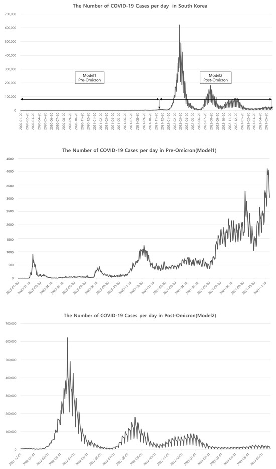
Figure 1. COVID-19 Infection Trends in South Korea.

Figure 2 illustrates our study area and the distribution of COVID-19 cases across the administrative districts (si-gun-gu) during the Pre-Omicron and Post-Omicron periods. The Seoul Metropolitan Area, located in the northwestern region of the country, exhibited a high concentration of cases in both periods, as indicated by the highest quantile of the case distribution. Other metropolitan areas also showed the high case levels. While the overall spatial patterns remained largely consistent between the two periods, some districts experienced changes in their relative case levels.

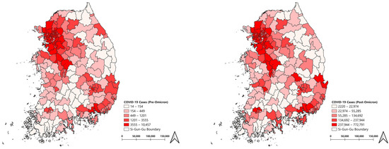
Figure 2. Spatial Distributions of COVID-19 Infections During the Pre-Omicron (left) and Post-Omicron (right) in South Korea.

2.2. Data and Variables

The multiple spatial datasets were measured at the si-gun-gu level as the unit of analysis in this study. The dependent variable was the cumulative number of confirmed COVID-19 cases across 226 si-gun-gu administrative districts from June 2021 to June 2022. The data on COVID-19 cases were collected from the official website published by the Korea Disease Control and Prevention Agency (https://dportal.kdca.go.kr/pot/is/summaryEDW.do, accessed on 10 July 2022). As recommended in the previous literature, control variables in this study included socioeconomic and demographic characteristics, such as average household income, employed population, population with college education or higher, smoking population, older population aged 65 or older, and foreign population. In addition, consumer sales amount, daily traffic volume, and cluster infection cases were included to control for economic activity, population mobility, and epidemiological risk, which have been linked to disease transmission [39,49,50]. The cluster infection variable was measured as a dummy indicating whether a cluster infection involving 100 or more people occurred. The control variables were assembled from various data sources, such as Statistical Geographic Information Service (for census-based socioeconomics and demographics), the Korea Transport Institute (for traffic volume), and National Information & Credit Evaluation (NICE) (for credit card sales data).

The main independent variables of our interest were various urban factors related to accessible and connected environments conceptualized within the widely recognized D-construct framework. The original D construct framework proposed by Cevero and Kockelman [51] as three Ds—i.e., density, diversity, and design–was later expaned to five Ds with the addition of destination accessibility and distance to transit [52]. In this current study, distance to transit was considered part of destination accessibility and we ultimately examined four Ds: density, diversity, design and destination accessibility.

Density was measured using various indicators per unit area, including residential density (number of residences), apartment density (number of apartments), business density (number of employees), traffic density (total traffic volumes), population density (total population per area) and floating pulation density. Diversity was measured as land-use mix based on the entropy index among residential, commercial, industrial and green land uses. Design was measured as street connectivity, calculated by the number of intersections per unit area or as the total length of street per unit area. The literature commonly relies on street network metrics because aesthetic aspects of design are difficult to measure [52,53]. Destination accessibility was measured as the number of destinations per the unit area, including educational, cultural, religious, community, commercial, business, and medical facilities, tourist-related acommodations, universities, supermarkets, and pharmacies. The data for these D variables were collected from various sources, including the Korea Transport Institute (street), Statistics Korea (land use), Korea National Spatial Data Information Portal (destinations), Statistical Geographic Information System (supermarkets), Higher Education (universities), Korea Educational Development Institute (proviate academies), and Korean Statistical Information Service (medical facilities and pharmacy). All datasets were used as geospatial data to measure variables in si-gun-gu administrative units using ArcGIS Pro.

2.3. Analytic Methods

2.3.1. Negative Binomial Regression

As our dependent variable is the number of confirmed COVID-19 cases per si-gun-gu administrative unit, we considered count regression models. Poisson regression or negative binomial regression (NBR) is widely used for modeling count data, particularly when the outcome variable represents the frequency of an event, such as infections [54]. The count response $y_i$ at observation $i$ is assumed to be a random variable from a Poisson distribution with expected count ${E\left(y_i\right)=\mu }_i$, and the probability of observing confirmed cases $y_i$ in a given si-gun-gu unit $i$ is expressed as:

$$P\left(Y_i=y_i\right)={\displaystyle \frac{\mathrm{e}\mathrm{x}\mathrm{p}(-{\mu }_i){{\mu }_i}^{y_i}}{y_i!}}.$$

Both Poisson regression and NBR belong to the generalized linear model (GLM) family, where the expected count ${\mu }_i$ is modeled as a function of explanatory variables. The popular functional form is exponential, which ensures nonnegative predicted outcome values. The expected count ${\mu }_i$ is also expressed as a linear combination of explanatory variables in a log-link function:

$$\begin{gathered} {\mu }_i=\exp \left(\alpha +{\mathit{Z}}_i\mathit{\gamma }+\beta x_i\right) \\ \mathrm{o}\mathrm{r} \\ ln\left({\mu }_i\right)=\alpha +{\mathit{Z}}_i\mathit{\gamma }+\beta x_i, \end{gathered}$$

where ${\mu }_i$ is the expected count of the count response, ${\mathit{Z}}_i$ is the matrix of control variables for the base model, $x_i$ is the independent variable to be tested for the built-environment effect, $\mathit{\gamma }$ and $\beta$ are the estimated coefficients. The exposure term defined as the natural logarithm of population across si-gun-gu units was included with a fixed coefficient of 1.

Poisson model assumes equal mean and variance; however, real-world data often exhibits overdispersion, where variance exceeds the mean, leading to inefficiency in model estimation [55]. NBR addresses this overdispersion by adding a random error term, ${\epsilon }_i$ with a coefficient of one in the model, which represents unobserved heterogeneity or additional randomness [54]:

$${\tilde{\mu }}_i=\exp \left(\alpha +{\mathit{Z}}_i\mathit{\gamma }+\beta x_i+{1\epsilon }_i\right)={\mu }_i\exp \left({\epsilon }_i\right)={\mu }_i{\mathrm{G}}_i,$$

where ${\mathrm{G}}_i=\exp \left({\epsilon }_i\right)$ follows a gamma distribution with mean ${\mathrm{E}(\mathrm{G}}_i)=1$ and variance $\theta$, i.e., $\mathrm{G}~\mathrm{g}\mathrm{a}\mathrm{m}\mathrm{m}\mathrm{a}({\theta }^{-1}, {\theta }^{-1})$. Substituting ${\tilde{\mu }}_i$ for ${\mu }_i$, the probability of $y_i$ is computed as the compound distribution weighted from the gamma distribution [54]:

$$P\left(Y_i=y_i\right)={\displaystyle \frac{\mathsf{\Gamma }(y_i+{\theta }^{-1})}{\mathsf{\Gamma }\left({\theta }^{-1}\right)y_i!}}{({\displaystyle \frac{\theta {\mu }_i}{1+{\theta \mu }_i}} )}^{y_i}{({\displaystyle \frac{1}{1+{\theta \mu }_i}} )}^{{\theta }^{-1}},$$

where $\theta$ is the dispersion parameter and $\mathsf{\Gamma }(·)$ is the gamma function. If $\theta =0$, meaning no overdispersion, the NBR model simplifies to the Poisson regression [54]. The parameters are typically estimated via maximum likelihood estimation (MLE).

In the analytic process, we first investigated overdispersion by comparing variance to mean and by conducting the likelihood-ratio (LR) test for the dispersion parameter $\alpha$. The overdispersed histogram and the significant LR test confirmed the appropriateness of NBR for our analysis. We conducted a series of bivariate analyses to identify the base model including significant sociodemographic control variables. We then examined the environmental effect by sequentially adding each variable from the D dimensions into the base model. In this study, we analyzed the early stage of COVID-19 based on the cumulative infections during the pre-Omicron period until 30 November 2021 as Model 1, and the post-Omicron period from 1 December 2021 to 13 June 2023 as Model 2.

2.3.2. Random Forest

We used Random Forest (RF), a popular ensemble model known for its strong performance in both academic research and data science applications. Ensemble models improve accuracy by combining multiple predictors (often dozens or hundreds) through voting, bagging, or boosting methods [56]. In bagging (short for bootstrap aggregating), predictors are generated using the same algorithm but with different data subsets obtained from sampling with replacement.

RF is typically constructed using the bagging method for the combination of decision tree (DT) predictors, where each predictor employs a random subset of m variables selected from the full set of p variables [57]. This random selection ensures that different trees are built using different subsets of variables, thereby reducing correlation between trees [57]. A DT is a tree-shaped structure that begins with an initial node (or a root node), which is then split into internal nodes that partition subsets of the data, ultimately leading to leaf nodes that represent the final prediction [58]. The splitting criterion at each node is selected to maximize the homogeneity within the resulting data partitions. For classification tasks, the optimal DT model is based on the Gini impurity or entropy index, both of which assess the homogeneity of the final classified data. For regression tasks, the DT model is built by minimizing the sum of squared difference between the observed value and the mean of observations within each partition.

The RF model follows a four-step procedure to achieve robust predictive performance while minimizing overfitting: (1) the bagged DTs are trained on approximately 80% of the dataset. Similar to the outcome used in the NBR models, the RF models utilized a rate calculated by dividing the total number of COVID-19 cases by the population. All independent variables were included for the RF model due to the model’s ability to handle many independent variables without multicollinearity; (2) the hyperparameters, including the number of trees, the number of variables, and the depth of the trees, are tuned using the Grid Search Python library to optimize the model performance [59]; (3) out-of-bag (OOB) data, which are samples excluded during bootstrapping, are used to evaluate model performance, and the model with the lowest prediction error rate is selected [58]; (4) the final RF model provides feature importance scores, which quantify each variable’s contribution to the overall prediction accuracy based on the total reduction in impurity for classification tasks or variance for regression tasks.

To interpret our RF models, we applied the Shapley Additive exPlanations (SHAP) method, introduced by Lundberg and Lee [60]. SHAP is based on the Shapley value, from Shapley’s cooperative game theory, which provides a fair and unique way to distribute payoffs (i.e., contributions) among players (i.e., model features) working toward a shared outcome [61,62]. In practice, SHAP evaluates an additive feature contribution to the model’s prediction by calculating a weighted average of feature’s marginal contribution across all possible feature combinations [60]. The SHAP is defined as the following equation:

$${\phi }_i=\sum _{S\in F\backslash \left\{i\right\}}{\displaystyle \frac{\left|S\right|!\left(\left|F\right|-\left|S\right|!-1\right)!}{\left|F\right|!}}\left[f_x\left(S\cup \left\{i\right\}\right)-f_x\left(S\right)\right] ,$$

where $F$ is the set of all features, $S$ is the subset of $F\backslash \left\{i\right\}$ which is a set of all possible combinations of features excluding the $i$th feature, $\left|F\right|$ and $\left|S\right|$ are the number of features in $F$ and $S$ respectively, and $f_x\left(S\right)=E\left[f\right(x\left)\right|x_s]$ is the conditional expectation of model output given the feature in subset $S$. All RF and SHAP analyses were conducted by using the scikit-learn (version 1.6.0) Python packages.

3. Results

3.1. Summary Statistics

Table 1 presents the summary statistics. The dependent variable, the cumulative confirmed cases averaged approximately 1873 with a range from 14 to 10,457 during the Pre-Omicron period (Model 1) and approximately 137,902 with a range from 2220 to 772,791 during the post-Omicron period (Model 2), which reflected the high transmission rate of the Omicron variant. In both periods, the standard deviations were greater than the means, indicating substantial variability. The variability was also found across socioeconomic and built-environment characteristics. For example, floating population density averaged 17.46 with a standard deviation of 27.48. Among the 226 si-gun-gu units, 22 (9.73%) reported clustered infections with over 100 cases in specific locations, while 90.28% did not report any cluster infection.

Table 1. Summary statistics of the variables.

Variable	Description	Mean/Freq.	S.D./% (Min.–Max.)
Dependent Variables
Pre-Omicron cases	Continuous: Cumulative COVID-19 cases before Omicron until 30 November 2021	1873.6500	2396.4900 (14–10,457)
Post-Omicron cases	Continuous: Cumulative COVID-19 cases after Omicron until 30 June 2023	137,902.1000	143,072.8000 (2220–772,791)
Socioeconomic Characteristics
Household income	Continuous: Average household income	35,589.3800	4788.4360 (3248–63,288)
Employed rate	Continuous: % of employed population	63.9239	6.2499 (49.3000–82.4000)
Education rate	Continuous: % of college graduate or higher education	2.5065	1.6876 (0.6823–11.1208)
Smoking	Continuous: % of smoking population	20.2779	2.9730 (11.8000–28.8000)
Traffic volume	Continuous: daily estimated traffic volume	274.5934	596.2259 (0.6546–5858.3040)
Older population	Continuous: % of population aged 65 plus	22.1743	8.3500 (3.4231–43.4788)
Foreign population	Continuous: % of foreigners	3.2871	2.5657 (0.4964–14.8081)
Local consumer sales	Continuous: Total sales by industry (Billion KRW)	25,295.8600	48,661.3400 (315.2601–461,390.90000)
Cluster infection	Binary: 0 = None 1 = Having a cluster infection of 100 or more people	0.0973	0.2971 (0–1)
Density
Floating population density	Continuous: total of floating population per si-gun-gu area	17.4688	27.4873 (0.0790–148.6046)
Net residential density	Continuous: total residential units per residential area within si-gun-gu area	33.3213	36.7886 (0.2669–129.4280)
Net apartment density	Continuous: total apartment units per housing unit within si-gun-gu area	0.5571	0.2864 (0.0054–0.9931)
Employment density	Continuous: total employments per si-gun-gu area	466.1570	940.4703 (2.0938–7598.6950)
Residential land uses	Continuous: total area of residential land uses per si-gun-gu area	22.1244	16.2235 (4.3900–91.5000)
Commercial land uses	Continuous: total area of commercial land uses per si-gun-gu area	3.1086	5.1217 (0.2300–44.2400)
Green land uses	Continuous: total area of green land uses per si-gun-gu area	0.6478	0.2112 (0.0025–0.9284)
Diversity
Land-use mix *	Continuous: the entropy-based land-use mix calculated as $-{\sum }_{i=1}^k\left({\displaystyle \frac{{(P}_i)\ast \ln (P_i)}{\ln \left(k\right)}}\right)$	0.6528	0.1709 (0.2504–0.9986)
Employment mix **	Continuous: entropy-based employment mix calculated as $-{\sum }_{i=1}^k\left({\displaystyle \frac{{(P}_i)\ast \ln (P_i)}{\ln \left(k\right)}}\right)$	0.9193	0.0402 (0.7327–0.9849)
Design
Road density	Continuous: total road length per si-gun-gu area	169.5991	215.6534 (1.400–1078.3400)
Street connectivity	Continuous: total number of street intersection per si-gun-gu area	1060.1060	1432.18 (3.300–6318.2000)
Destination Accessibility
Educational facilities	Continuous: total number of educational facilities per si-gun-gu area	2.7958	4.0450 (0.0478–20.2183)
Cultural facilities	Continuous: total number of cultural facilities per si-gun-gu area	0.3821	0.9914 (0.0143–12.3379)
Religious facilities	Continuous: total number of religious facilities per si-gun-gu area	1.5102	2.0442 (0.0480–12.3230)
Office facilities	Continuous: total number of office facilities per si-gun-gu area	1.4538	3.4326 (0.0047–26.5018)
Community facilities	Continuous: total number of community facilities per si-gun-gu area	52.9773	99.0031 (0.9556–753.0035)
Medical facilities	Continuous: total number of medical facilities per si-gun-gu area	3.3086	6.4818 (0–47.4177)
Pharmacy stores	Continuous: total number of pharmacy stores per si-gun-gu area	2.1073	3.7654 (0.0036–21.6714)

Note: N = 226. * The land-use mix was calculated as $-{\sum }_{i=1}^k\left({\displaystyle \frac{{(P}_i)\ast \ln (P_i)}{\ln \left(k\right)}}\right)$, where $P_i$ = subject land uses (residential, commercial, industrial or green) divided by total area of subject land uses within each si-gun-gu, and $k$ = number of land uses present. ** The employment mix was calculated as $-{\sum }_{i=1}^k\left({\displaystyle \frac{{(P}_i)\ast \ln (P_i)}{\ln \left(k\right)}}\right)$, where $P_i$ = subject employment types (office, retail, industrial, service, or entertainment) divided by total number of employment types within each si-gun-gu, and $k$ = number of employments present.

3.2. Empirical Results from Negative Binomial Regression Analysis

3.2.1. Base Model

Table 2 presents the results of the base model. In Model 1 for the Pre-Omicron period, the results showed that the si-gun-gu areas with higher household income, a larger employed population, and an older population were negatively associated with the COVID-19 cases. In contrast, the areas with a larger population holding graduate degrees, more traffic volumes, a larger smoking population, and a larger foreign population showed a positive association with the COVID-19 cases. In the Model 2 for the Post-Omicron period, education level, traffic volume, elderly population, and foreign population were only found to be significant with smaller coefficient sizes than those in the Pre-Omicron model. Local consumption was not significant in either period. Clustered infection was significant at the 0.1 level in the Model 1 but insignificant in the Model 2.

Table 2. Base Model.

Variables	Pre-Omicron (Model 1)			Post-Omicron (Model 2)
	Coeff.	S.E.	p-Value	Coeff.	S.E.	p-Value
Socioeconomic Characteristics
Household income	−2.68 × 10−5	1.03 × 10−5	0.0090	−3.45 × 10−6	3.67 × 10−6	0.3470
Employment	−0.0194	0.0071	0.0060	−0.0016	0.0023	0.4950
Smoking	0.0311	0.0118	0.0080	−0.0054	0.0040	0.1720
Education	0.1679	0.0350	0.0000	0.0259	0.0106	0.0150
Traffic Volume	0.0002	0.0001	0.0070	3.69 × 10−5	1.86 × 10−5	0.0470
Older population	−0.0238	0.0055	<0.0001	−0.0132	0.0018	<0.0001
Foreign population	0.0744	0.0121	0.0000	0.0094	0.0040	0.0190
Local consumer sales	3.95 × 10−7	7.83 × 10−7	0.6140	3.65 × 10−8	2.50 × 10−7	0.0884
Cluster Infection	0.1825	0.1014	0.0720	−0.0175	0.0335	0.6010
Model Summary
Number of Obs.	226			226
LR Chi2	193.06			159.21
$\alpha$ [95% confidence interval]	0.1908 [0.1590, 0.2290]			0.2111 [0.0176, 0.0254]
LR test of $\alpha$	5.2 × 105			4.0 × 105
AIC	3279.79			4877.90

Note: The VIF (variance inflation factor) values are 1.19 (average) and 2.19 (maximum) for the Pre-Omicron analysis and 1.19 (average) and 2.19 (maximum) for the Post-Omicron analysis.

The negative binomial regression was identified as the best fit for our data. The LR Chi2 tests had values of 193.06 for Model 1 and 159.21 for Model 2, both statistically significant with p-values below 0.001. The estimated dispersion parameter ($\alpha$) was significantly greater than zero in both models, and the LR tests for overdispersion were also statistically significant.

3.2.2. Adjusted Model for Built Environments

Table 3 shows the results of the adjusted model that examines environmental effect on COVID-19 case, controlling for the base model. Density-related factors were consistently significant across both Pre- and Post-Omicron periods while specific variables as well as magnitude and direction of their associations differed between the two periods. Floating population density, residential density, and commercial land use density were significant predictors of COVID-19 cases in both periods. However, floating population density and apartment density were only significant in the Pre-Omicron period, while overall employment levels were significant in the Post-Omicron period. The directions of association of residential density and commercial land use density differed between Pre- and Post-Omicron models. The areas with a higher density of residential units were positively related to more COVID-19 cases during the Pre-Omicron period but were negatively related to cases in the Post-Omicron period. In contrast, commercial land use density showed the negative direction in the Pre-Omicron model and the positive association with COVID-19 cases in the Post-Omicron model.

Table 3. Adjusted One-by-One Model.

Variables	Pre-Omicron (Model 1)			Post-Omicron (Model 2)
	Coeff.	S.E.	p-Value	Coeff.	S.E.	p-Value
Density
Floating population density	0.0076	0.0024	0.0015	−0.0012	0.0008	0.1072
Net residential density	0.0037	0.0013	0.0043	−0.0019	0.0004	<0.0001
Net apartment density	1.6732	0.3097	<0.0001	0.0035	0.1086	0.9744
Employment density	0.0001	7.27 × 10−5	0.2802	0.0001	2.08 × 10−5	0.0140
Residential land uses	0.0099	0.0024	0.0001	−0.001	0.0008	0.5489
Commercial land uses	−0.0171	0.0082	0.0363	0.0146	0.0028	<0.0001
Green land uses	−0.0580	0.2040	0.7760	−0.0597	0.0642	0.3522
Diversity
Land use mix	−0.0477	0.1891	0.8007	0.0745	0.0626	0.2340
Employment mix	1.1564	0.8842	0.1909	−0.4553	0.3165	0.1502
Design
Road density	−4.34 × 10−5	0.0002	0.8176	0.0001	0.0001	0.1252
Street connectivity	3.22 × 10−5	3.13 × 10−5	0.3036	1 × 10−5	1 × 10−5	0.4437
Destination Accessibility
Educational facilities	0.0271	0.0133	0.0408	−0.0075	0.0042	0.0713
Cultural facility	−0.0323	0.0350	0.3568	0.0278	0.0118	0.0177
Religious facility	0.0983	0.0312	0.0016	−0.0205	0.0104	0.0496
Office facility	−0.0014	0.0135	0.9191	−0.0003	0.0044	0.9382
Community facility	4.01 × 10−5	0.0008	0.9586	0.0005	0.0002	0.0278
Medical facilities	0.0250	0.0092	0.0068	−0.0021	0.0029	0.4811
Pharmacy stores	0.0557	0.0163	0.0006	−0.0033	0.0054	0.5419

Regarding diversity and design factors, no variables were found to be significant. Regarding destination accessibility, educational facilities, medical facilities, and pharmacy stores were significantly associated with the COVID during the Pre-Omicron period, whereas cultural and commercial facilities were significant in the Post-Omicron period. Religious facilities and sales facilities were significant in both periods, though the direction of coefficients differed across the periods.

3.3. Empirical Results from Random Forest Analysis

Table 4 shows the feature importances derived from the Random Forest (RF) models. Overall, factors including residential density, medical facility, pharmacy store, population with higher education attainment, older population, and local consumer sales consistently emerged as important across the RF models, while importance of other variables varied between two periods. During the Pre-Omicron period, the RF model identified residential land use density as the most important factor, and others ranked among ten important factors included traffic volume density, foreign population, and smoking population. In the Post-Omicron period, the older population variable was the most important factor and others not overlapped in the Pre-Omicron period included household income, employment rate, cultural facility and commercial land use.

Table 4. Random Forest Model.

	Pre-Omicron (Model 1)		Post-Omicron (Model 2)
Variable	Rank	Feature Importance	Rank	Feature Importance
Household Income	18	0.000047	4	0.009669
Employment Rate	12	0.000097	6	0.009218
Smoking Population	7	0.000268	23	0.000760
Education Rate	9	0.000223	9	0.004357
Traffic Volume	3	0.000453	17	0.001206
Older Population	6	0.000380	1	0.033028
Foreign Population	4	0.000440	16	0.001214
Local Consumer Sales	10	0.000165	11	0.002250
Cluster Infection	27	0.000005	27	0.000057
Floating Population Density	17	0.000059	20	0.001020
Net Residential Density	21	0.000040	10	0.002455
Net Apartment Density	5	0.000425	2	0.011835
Employment Density	16	0.000067	21	0.000976
Residential Land Use	1	0.000834	19	0.001100
Commercial Land Use	14	0.000072	8	0.005710
Green Land Use	25	0.000026	13	0.001605
Land Use Mix	20	0.000043	25	0.000652
Employment Mix	13	0.000073	14	0.001291
Road Density	26	0.000026	24	0.000718
Street Connectivity	22	0.000040	18	0.001140
Educational Facilities	24	0.000028	12	0.002105
Cultural Facilities	23	0.000031	7	0.008153
Religious Facilities	19	0.000044	15	0.001237
Office Facilities	15	0.000069	26	0.000583
Medical facilities	2	0.000462	5	0.009388
Community Facilities	11	0.000163	22	0.000773
Pharmacy Stores	8	0.000250	3	0.009952

The SHAP plots provided further insight into the associations between key factors and COVID-19 cases (Figure 3). In the Pre-Omicron period, variables such as residential land use, foreign population, apartment density, medical facilities, smoking population, and pharmacy stores seemed to be positively associated with COVID-19 cases, while the older population variable showed a likely negative association with the cases. Some factors such as traffic volume showed mixed, purple colors across SHAP values, indicating a lack of significant associations. In the Post-Omicron model, most of the top ranked factors showed mixed colors within the positive SHAP values. However, older population, apartment density, and household income displayed some clearer distinct color patterns across SHAP values. Specifically, the population aged 65 and over exhibited red shading for low SHAP values and blue shading for high SHAP values, suggesting a negative association with COVID-19 cases. This indicates that the areas with more elderly residents tended to have fewer COVID-19 cases.

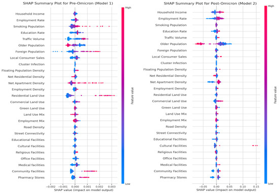
Figure 3. SHAP Summary Plots.

4. Discussion and Conclusions

4.1. Discussion

The interplay between urban environment and infectious disease transmission has garnered attention since the onset of the COVID-19 pandemic. However, previous studies have focused narrowly on density measures, with limited attention to the varied roles of different built-environment dimensions and different epidemiological phases of the pandemic. This study aimed to examine the effects of various urban factors conceptualized in the D-variable framework on COVID-19 transmission in South Korea. By analyzing both pre- and post-Omicron periods, integrating various GIS measures with so-called big data (from Wi-Fi, GPS, and credit card transaction), and employing negative binomial regression and random forest models, this study provides new insights into the complex interplay between urban environments and the spread of COVID-19.

Our results consistently emphasize the importance of density-related factors such as population, residential, and apartment density in driving COVID-19 transmission across both pandemic phases and analytic approaches. This finding reinforces the notion that urban density is a key determinant of infection risk with high density facilitating virus transmission through increased contacts, as suggested in the literature [18,23,25,35,36]. However, we found that specific significant variables varied across periods and analytic models. For example, while residential and population densities (as identified by the NBR model) and residential land use (as identified by the RF model) were significant during the pre-Omicron period, employment level (identified as employment density in the NBR and employment rate in the RF) emerged as significant factors in both models. This result may reflect the findings from previous studies, which suggest that denser and more populous areas were initially linked to higher COVID-19 transmission, but the relationship weakened over time as mobility patterns and economic activities changed [11,36,43,63]. Instead, density factors associated with higher interaction exposure, such as workplaces and commercial centers, became stronger predictors of COVID-19 risks in later phases [35,36].

The differences in significant variables across periods may help explain the inconsistencies regarding density effects reported in the literature and highlight the importance of investigating multiple density measures and time points [15,19]. Furthermore, our findings suggest that broader urban contexts moderate the relationship between density and disease transmission. Previous studies were conducted in diverse geographic regions across America, Europe, Asia, and Africa with varying scopes of study areas [15,39]. The mixed findings on density in the literature might be attributable to variations in localities, subpopulations, socioeconomic conditions, and the quality of infrastructure and services. For example, apartment density, which represents distinctive housing landscape of South Korea, was found to be significant in this study. Such urban contexts may differ from those more commonly studied in the United States, where suburban and low-density environments yield different density effects.

Destination accessibility factors also varied by pandemic periods and analytic models. While education facilities and hospitals were significant during the pre-Omicron period, destinations relating to social and economic activities such as cultural, commercial and sales facilities appeared to be important during the post-Omicron period. The random forest models also showed local consumption sales amount as an important factor in the later phase, suggesting that local economic activities are associated with virus transmission. Previous research has found that high-contact venues, such as shops, gyms, museums, and restaurants, tend to attract dense crowds and have more face-to-face contact, increasing the likelihood of viral spread [36,64]. Different significant venues between the periods might reflect changes in policy measures, such as modifications in social distancing or capacity limits. Previous research has shown that the reopening of such venues, which boost consumers’ activities, was significantly related to COVID-19 transmission [65]. Unexpectedly, inconsistent with the literature [20,63], land-use mix and street connectivity were not statistically significant and not ranked as more important factors in our study. The current measures or available data for urban diversity and design might be insufficient to fully capture these dimensions, calling for more sophisticated data and analytical strategies. In addition, our results might be explained by the potential interplay among various urban factors used in this study, as previous urban studies have examined direct and indirect relationships among urban form, land uses, and, mobility [5,52].

Our findings showed the significant role of socioeconomic and demographic factors. Consistent with previous findings [22,24,30,42,66], higher levels of household income and older population were consistently associated with lower COVID-19 cases and were ranked as important factors. Higher levels of traffic volume, foreign population, and educated population were significantly associated with more COVID-19 cases, indicating that exposure risk through mobility, cross-border interactions, and educational activities increased virus transmission. Some variables were not found to be important in the random forest models. Because the random forest captures more non-linearities and high-order interactions across various variables without certain functional form assumptions [46,48], the predictive contribution of some variables might be small when the variables were not important and conversely, some variables with non-linearity can appear to be important when the variables were not statistically significant.

This study is subject to several limitations. First, we relied on aggregated COVID-19 case data at the si-gun-gu (administrative unit) level. As noted by previous studies [18], such aggregated data may obscure local heterogeneities. Future investigation needs to employ finer-scale datasets to yield more context-specific insights into complex urban environments. Second, while this study employed multiple analytical approaches including regression-based and machine learning-based methods, the findings can be addressed based on national-level average effects. Recognizing that environmental determinants and their impacts may vary by locality, future analysis needs to consider spatially detailed COVID-19 data and fine-grained environmental variables to better capture transmission dynamics. Third, this study did not account for non-pharmaceutical policies (e.g., social distancing) which were applied inconsistently during the post-Omicron period. Lastly, the use of cross-sectional data precludes causal inferences. Future study should utilize longitudinal datasets to strengthen causal interpretations.

4.2. Conclusions

The findings of this study contribute to the literature on urban environments and public health by providing a more nuanced understanding of how diverse urban environments were associated with COVID-19 transmission across distinct pandemic phases. The results highlight the need for adaptive urban planning strategies that consider the evolving nature of the pandemic and the shifting importance of various urban characteristics over time. While urban density consistently played a prominent role in COVID-19 transmission, the specific density factors varied between the early and later pandemic phases. In the early phase, static urban density characteristics such as population and residential density appeared more significant, but dynamic urban density characteristics such as employment and commercial activity became more significant in the later phase. Our findings suggest that urban planning strategies need to go beyond traditional interventions based on population density and adopt a multifaceted, adaptive approach that considers urban form, land use, economic activity, and mobility factors. Policy makers should consider both static and dynamic urban characteristics when developing policy strategies to minimize the risk of infectious diseases while promoting urban vitality and health.

References

- Johns Hopkins Coronavirus Research Center. COVID-19 Dashboard. 2023. Available online: https://coronavirus.jhu.edu/map.html (accessed on 10 March 2023).
- Antras, P.; Redding, S.J.; Rossi-Hansberg, E. Globalization and Pandemics. Am. Econ. Rev. 2023, 113, 939–981. [Google Scholar] [CrossRef]
- Tatem, A.J.; Rogers, D.J.; Hay, S.I. Global Transport Networks and Infectious Disease Spread. Adv. Parasitol. 2006, 62, 293–343. [Google Scholar] [CrossRef] [PubMed]
- Flaxman, S.; Mishra, S.; Gandy, A.; Unwin, H.J.T.; Mellan, T.A.; Coupland, H.; Whittaker, C.; Zhu, H.; Berah, T.; Eaton, J.W.; et al. Estimating the effects of non-pharmaceutical interventions on COVID-19 in Europe. Nature 2020, 584, 257–261. [Google Scholar] [CrossRef] [PubMed]
- Dannenberg, A.L.; Frumkin, H.; Jackson, R.J. Making Healthy Places: Designing and Building for Health, Well-Being, and Sustainability; Island Press: Washington, DC, USA, 2011. [Google Scholar]
- Frank, L.D.; Sallis, J.F.; Conway, T.L.; Chapman, J.E.; Saelens, B.E.; Bachman, W. Many Pathways from Land Use to Health. J. Am. Plan. Assoc. 2006, 72, 75–87. [Google Scholar] [CrossRef]
- Giles-Corti, B.; Vernez-Moudon, A.; Reis, R.; Turrell, G.; Dannenberg, A.L.; Badland, H.; Foster, S.; Lowe, M.; Sallis, J.F.; Stevenson, M.; et al. City planning and population health: A global challenge. Lancet 2016, 388, 2912–2924. [Google Scholar] [CrossRef]
- Mazumdar, S.; Learnihan, V.; Cochrane, T.; Davey, R. The Built Environment and Social Capital: A Systematic Review. Environ. Behav. 2018, 50, 119–158. [Google Scholar] [CrossRef]
- Won, J.; Lee, C.; Li, W. Are Walkable Neighborhoods More Resilient to the Foreclosure Spillover Effects? J. Plan. Educ. Res. 2018, 38, 463–476. [Google Scholar] [CrossRef]
- Karim, S.A.; Chen, H.-F. Deaths From COVID-19 in Rural, Micropolitan, and Metropolitan Areas: A County-Level Comparison. J. Rural Health 2021, 37, 124–132. [Google Scholar] [CrossRef]
- Carozzi, F.; Provenzano, S.; Roth, S. Urban density and COVID-19: Understanding the US experience. Ann. Reg. Sci. 2024, 72, 163–194. [Google Scholar] [CrossRef]
- Hazarie, S.; Soriano-Paños, D.; Arenas, A.; Gómez-Gardeñes, J.; Ghoshal, G. Interplay between population density and mobility in determining the spread of epidemics in cities. Commun. Phys. 2021, 4, 191. [Google Scholar] [CrossRef]
- Rader, B.; Scarpino, S.V.; Nande, A.; Hill, A.L.; Adlam, B.; Reiner, R.C.; Pigott, D.M.; Gutierrez, B.; Zarebski, A.E.; Shrestha, M.; et al. Crowding and the shape of COVID-19 epidemics. Nat. Med. 2020, 26, 1829–1834. [Google Scholar] [CrossRef]
- Ribeiro, H.V.; Sunahara, A.S.; Sutton, J.; Perc, M.; Hanley, Q.S. City size and the spreading of COVID-19 in Brazil. PLoS ONE 2020, 15, e0239699. [Google Scholar] [CrossRef] [PubMed]
- Sharifi, A.; Khavarian-Garmsir, A.R. The COVID-19 pandemic: Impacts on cities and major lessons for urban planning, design, and management. Sci. Total Environ. 2020, 749, 142391. [Google Scholar] [CrossRef] [PubMed]
- Megahed, N.A.; Ghoneim, E.M. Antivirus-built environment: Lessons learned from COVID-19 pandemic. Sustain. Cities Soc. 2020, 61, 102350. [Google Scholar] [CrossRef]
- Bereitschaft, B.; Scheller, D. How Might the COVID-19 Pandemic Affect 21st Century Urban Design, Planning, and Development? Urban Sci. 2020, 4, 56. [Google Scholar] [CrossRef]
- Han, Y.; Yang, L.; Jia, K.; Li, J.; Feng, S.; Chen, W.; Zhao, W.; Pereira, P. Spatial distribution characteristics of the COVID-19 pandemic in Beijing and its relationship with environmental factors. Sci. Total Environ. 2021, 761, 144257. [Google Scholar] [CrossRef] [PubMed]
- Hong, A.; Chakrabarti, S. Compact living or policy inaction? Effects of urban density and lockdown on the COVID-19 outbreak in the US. Urban Stud. 2023, 60, 1588–1609. [Google Scholar] [CrossRef]
- Jo, Y.; Hong, A.; Sung, H. Density or Connectivity: What Are the Main Causes of the Spatial Proliferation of COVID-19 in Korea? Int. J. Environ. Res. Public Health 2021, 18, 5084. [Google Scholar] [CrossRef]
- Kim, M.; Park, I.H.; Kang, Y.S.; Kim, H.; Jhon, M.; Kim, J.W.; Ryu, S.; Lee, J.Y.; Kim, J.M.; Lee, J.; et al. Comparison of Psychosocial Distress in Areas With Different COVID-19 Prevalence in Korea. Front. Psychiatry 2020, 11, 593105. [Google Scholar] [CrossRef]
- Lee, W.; Kim, H.; Choi, H.M.; Heo, S.; Fong, K.C.; Yang, J.; Park, C.; Kim, H.; Bell, M.L. Urban environments and COVID-19 in three Eastern states of the United States. Sci. Total Environ. 2021, 779, 146334. [Google Scholar] [CrossRef]
- Li, B.; Peng, Y.; He, H.; Wang, M.S.; Feng, T. Built environment and early infection of COVID-19 in urban districts: A case study of Huangzhou. Sustain. Cities Soc. 2021, 66, 102685. [Google Scholar] [CrossRef] [PubMed]
- Li, S.J.; Ma, S.; Zhang, J.Y. Association of built environment attributes with the spread of COVID-19 at its initial stage in China. Sustain. Cities Soc. 2021, 67, 102752. [Google Scholar] [CrossRef] [PubMed]
- Wong, D.W.S.; Li, Y. Spreading of COVID-19: Density matters. PLoS ONE 2020, 15, e0242398. [Google Scholar] [CrossRef] [PubMed]
- Xu, G.; Jiang, Y.H.; Wang, S.; Qin, K.; Ding, J.C.; Liu, Y.; Lu, B.B. Spatial disparities of self-reported COVID-19 cases and influencing factors in Wuhan, China. Sustain. Cities Soc. 2022, 76, 103485. [Google Scholar] [CrossRef] [PubMed]
- You, H.Y.; Wu, X.; Guo, X.X. Distribution of COVID-19 Morbidity Rate in Association with Social and Economic Factors in Wuhan, China: Implications for Urban Development. Int. J. Environ. Res. Public Health 2020, 17, 3417. [Google Scholar] [CrossRef]
- Hamidi, S.; Hamidi, I. Subway Ridership, Crowding, or Population Density: Determinants of COVID-19 Infection Rates in New York City. Am. J. Prev. Med. 2021, 60, 614–620. [Google Scholar] [CrossRef]
- Barak, N.; Sommer, U.; Mualam, N. Urban attributes and the spread of COVID-19: The effects of density, compliance and socio-political factors in Israel. Sci. Total Environ. 2021, 793, 148626. [Google Scholar] [CrossRef]
- Hamidi, S.; Sabouri, S.; Ewing, R. Does Density Aggravate the COVID-19 Pandemic? Early Findings and Lessons for Planners. J. Am. Plan. Assoc. 2020, 86, 495–509. [Google Scholar] [CrossRef]
- Hamidi, S.; Ewing, R.; Sabouri, S. Longitudinal analyses of the relationship between development density and the COVID-19 morbidity and mortality rates: Early evidence from 1,165 metropolitan counties in the United States. Health Place 2020, 64, 102378. [Google Scholar] [CrossRef]
- Khavarian-Garmsir, A.R.; Sharifi, A.; Moradpour, N. Are high-density districts more vulnerable to the COVID-19 pandemic? Sustain. Cities Soc. 2021, 70, 102911. [Google Scholar] [CrossRef]
- Spotswood, E.N.; Benjamin, M.; Stoneburner, L.; Wheeler, M.M.; Beller, E.E.; Balk, D.; McPhearson, T.; Kuo, M.; McDonald, R.I. Nature inequity and higher COVID-19 case rates in less-green neighbourhoods in the United States. Nat. Sustain. 2021, 4, 1092–1098. [Google Scholar] [CrossRef]
- Venerandi, A.; Aiello, L.M.; Porta, S. Urban form and COVID-19 cases and deaths in Greater London: An urban morphometric approach. Environ. Plan. B Urban Anal. City Sci. 2022, 50, 1228–1243. [Google Scholar] [CrossRef] [PubMed]
- Almagro, M.; Orane-Hutchinson, A. JUE Insight: The determinants of the differential exposure to COVID-19 in New York city and their evolution over time. J. Urban Econ. 2022, 127, 103293. [Google Scholar] [CrossRef] [PubMed]
- Verma, R.; Yabe, T.; Ukkusuri, S. Spatiotemporal contact density explains the disparity of COVID-19 spread in urban neighborhoods. Sci. Rep. 2021, 11, 10952. [Google Scholar] [CrossRef] [PubMed]
- Adlakha, D.; Higgs, C.; Sallis, J.F. Growing evidence that physical activity-supportive neighbourhoods can mitigate infectious and non-communicable diseases. Cities Health 2024, 8, 544–553. [Google Scholar] [CrossRef]
- Li, W.; Li, J.; Yi, J. Government management capacities and the containment of COVID-19: A repeated cross-sectional study across Chinese cities. BMJ Open 2021, 11, e041516. [Google Scholar] [CrossRef]
- Alidadi, M.; Sharifi, A. Effects of the built environment and human factors on the spread of COVID-19: A systematic literature review. Sci. Total Environ. 2022, 850, 158056. [Google Scholar] [CrossRef]
- Brownson, R.C.; Hoehner, C.M.; Day, K.; Forsyth, A.; Sallis, J.F. Measuring the built environment for physical activity: State of the science. Am. J. Prev. Med. 2009, 36, S99–S123.e12. [Google Scholar] [CrossRef]
- Frank, L.D.; Wali, B. Treating two pandemics for the price of one: Chronic and infectious disease impacts of the built and natural environment. Sustain. Cities Soc. 2021, 73, 103089. [Google Scholar] [CrossRef]
- Wali, B.; Frank, L.D. Neighborhood-level COVID-19 hospitalizations and mortality relationships with built environment, active and sedentary travel. Health Place 2021, 71, 102659. [Google Scholar] [CrossRef]
- Sun, Y.R.; Xie, J.; Hu, X.K. Detecting Spatial Clusters of Coronavirus Infection Across London During the Second Wave. Appl. Spat. Anal. Policy 2022, 15, 557–571. [Google Scholar] [CrossRef] [PubMed]
- Glaeser, E.L.; Gorback, C.; Redding, S.J. How Much Does COVID-19 Increase with Mobility? Evidence from New York and Four Other U.S. Cities. J. Urban Econ. 2022, 127, 103292. [Google Scholar] [CrossRef] [PubMed]
- Tsuboi, K.; Fujiwara, N.; Itoh, R. Influence of trip distance and population density on intra-city mobility patterns in Tokyo during COVID-19 pandemic. PLoS ONE 2022, 17, e0276741. [Google Scholar] [CrossRef] [PubMed]
- Mullainathan, S.; Spiess, J. Machine Learning: An Applied Econometric Approach. J. Econ. Perspect. 2017, 31, 87–106. [Google Scholar] [CrossRef]
- Yeşilkanat, C.M. Spatio-temporal estimation of the daily cases of COVID-19 in worldwide using random forest machine learning algorithm. Chaos Solitons Fractals 2020, 140, 110210. [Google Scholar] [CrossRef]
- Grekousis, G.; Feng, Z.; Marakakis, I.; Lu, Y.; Wang, R. Ranking the importance of demographic, socioeconomic, and underlying health factors on US COVID-19 deaths: A geographical random forest approach. Health Place 2022, 74, 102744. [Google Scholar] [CrossRef]
- Kraemer, M.U.G.; Yang, C.-H.; Gutierrez, B.; Wu, C.-H.; Klein, B.; Pigott, D.M.; Open COVID-19 Data Working Group; du Plessis, L.; Faria, N.R.; Li, R.; et al. The effect of human mobility and control measures on the COVID-19 epidemic in China. Science 2020, 368, 493–497. [Google Scholar] [CrossRef]
- Liu, T.; Gong, D.; Xiao, J.; Hu, J.; He, G.; Rong, Z.; Ma, W. Cluster infections play important roles in the rapid evolution of COVID-19 transmission: A systematic review. Int. J. Infect. Dis. 2020, 99, 374–380. [Google Scholar] [CrossRef]
- Cervero, R.; Kockelman, K. Travel demand and the 3Ds: Density, diversity, and design. Transp. Res. Part D Transp. Environ. 1997, 2, 199–219. [Google Scholar] [CrossRef]
- Ewing, R.; Cervero, R. Travel and the Built Environment. J. Am. Plan. Assoc. 2010, 76, 265–294. [Google Scholar] [CrossRef]
- Ramsey, K.; Bell, A. The smart location database: A nationwide data resource characterizing the built environment and destination accessibility at the neighborhood scale. Cityscape 2014, 16, 145–162. [Google Scholar]
- Hilbe, J.M. Negative Binomial Regression, 2nd ed.; Cambridge University Press: Cambridge, UK, 2011. [Google Scholar]
- Cameron, A.C.; Trivedi, P.K. Regression Analysis of Count Data; Cambridge University Press: Cambridge, UK, 2013. [Google Scholar]
- Rokach, L. Ensemble-based classifiers. Artif. Intell. Rev. 2010, 33, 1–39. [Google Scholar] [CrossRef]
- Breiman, L. Random forests. Mach. Learn. 2001, 45, 5–32. [Google Scholar] [CrossRef]
- James, G.; Witten, D.; Hastie, T.; Tibshirani, R.; Taylor, J. An Introduction to Statistical Learning: With Applications in Python; Springer Nature: Berlin/Heidelberg, Germany, 2023. [Google Scholar]
- Géron, A. Hands-On Machine Learning with Scikit-Learn, Keras, and TensorFlow, 2nd ed.; O’Reilly Media, Inc.: Sebastopol, CA, USA, 2019. [Google Scholar]
- Lundberg, S.M.; Lee, S.-I. A Unified Approach to Interpreting Model Predictions. In Proceedings of the Advances in Neural Information Processing Systems 30 (NIPS 2017), Long Beach, CA, USA, 4–9 December 2017; Curran Associates Inc.: Red Hook, NY, USA, 2017; Volume 30. [Google Scholar]
- Shapley, L.S. A Value for n-Person Games. In Contribution to the Theory of Games II; Kuhn, H.W., Tucker, A.W., Eds.; Princeton University Press: Princeton, NJ, USA, 1953; Volume 2, pp. 307–317. [Google Scholar]
- Štrumbelj, E.; Kononenko, I. Explaining prediction models and individual predictions with feature contributions. Knowl. Inf. Syst. 2014, 41, 647–665. [Google Scholar] [CrossRef]
- Zhang, A.; Shi, W.; Tong, C.; Zhu, X.; Liu, Y.; Liu, Z.; Yao, Y.; Shi, Z. The fine-scale associations between socioeconomic status, density, functionality, and spread of COVID-19 within a high-density city. BMC Infect. Dis. 2022, 22, 274. [Google Scholar] [CrossRef]
- Benzell, S.G.; Collis, A.; Nicolaides, C. Rationing social contact during the COVID-19 pandemic: Transmission risk and social benefits of US locations. Proc. Natl. Acad. Sci. USA 2020, 117, 14642–14644. [Google Scholar] [CrossRef]
- O’Donoghue, A.; Dechen, T.; Pavlova, W.; Boals, M.; Moussa, G.; Madan, M.; Thakkar, A.; DeFalco, F.J.; Stevens, J.P. Reopening businesses and risk of COVID-19 transmission. npj Digit. Med. 2021, 4, 51. [Google Scholar] [CrossRef]
- Hawkins, R.B.; Charles, E.J.; Mehaffey, J.H. Socio-economic status and COVID-19–related cases and fatalities. Public Health 2020, 189, 129–134. [Google Scholar] [CrossRef]
Disclaimer/Publisher’s Note: The statements, opinions and data contained in all publications are solely those of the individual author(s) and contributor(s) and not of MDPI and/or the editor(s). MDPI and/or the editor(s) disclaim responsibility for any injury to people or property resulting from any ideas, methods, instructions or products referred to in the content. |
© 2025 by the authors. Licensee MDPI, Basel, Switzerland. This article is an open access article distributed under the terms and conditions of the Creative Commons Attribution (CC BY) license (https://creativecommons.org/licenses/by/4.0/).