A Stochastic Multi-Objective Model for Optimal Design of Electronic Waste Reverse Supply Chain
Abstract
1. Introduction
2. Literature Review
2.1. Deterministic and Fuzzy RSC Design on E-Waste
2.2. Stochastic RSC Design on E-Waste
3. Model Development
3.1. Assumptions
3.2. Notations
3.3. Model Formulation
3.3.1. Model Objectives
- (a)
- Maximizing the total profit gained by implementing RSC of e-waste. To construct this objective function, revenues and costs are formulated as follows:
- (i)
- Revenues
- (ii)
- Total Costs
- 1-
- Construction costs
- 2-
- Processing costs
- a.
- Collection and sorting
- b.
- Refurbishing
- c.
- Disassembly
- d.
- Repair
- e.
- Material extraction
- f.
- Material recycling
- 3-
- Transportation costs
- (1)
- Transportation g→e
- (2)
- Transportation e→b
- (3)
- Transportation e→d
- (4)
- Transportation d→i
- (5)
- Transportation d→m
- (6)
- Transportation d→y
- (7)
- Transportation m→y and y→l
- (b)
- Minimizing total CO2 emissions
- CO2 emissions from refurbishing and disassembly
- 2.
- CO2 emissions from repair and material extraction
- 3.
- CO2 emissions from material recycling
- 4.
- CO2 emissions from transportation
- (c)
- Maximizing the social impact
- (1)
- Job opportunities
- (2)
- Lost days due to work-related injuries
3.3.2. Model Constraints
- ▪
- The total of QFjfgts (f→g) of product j sent from the consumer area f to the waste generation g is equal to the total QGjgets (g→e) of product j during period t at case s. That is,
- ▪
- The total of QFjfgts is equal to the sum of the totals of moved quantities QBjebts (e→d) and QEjedts (e→b) during period t at each case s. Mathematically,
- ▪
- The total QBjebts (e→b) of product j moved from station e to b is equal to the total QNjbnts (b→n) transported from station b to secondhand market n during period t at case s, as expressed in Equation (43).
- ▪
- At each case s, the total QIjcdits (d→i) of part c from product j transferred from disassembly station d to i is equal to the total QKjcikts (i→k) transported from station i to spare market k during period t at case s, as stated in Equation (44).
- ▪
- The sum of the totals QMjamyts and QYjadyts of material a in product j that is collected at both the material extraction station m and disassembly station d, respectively, and then transferred to the material recycling station y is equal to the sum of the totals QZjayzts and QLjaylts sent from material recycling station y to both raw material market z and landfill l, respectively, as formulated in Equation (45).
- ▪
- Let ZGgt be a binary variable that indicates whether or not the waste generation point g is opened, where a value of one indicates that waste generation g is opened and 0 otherwise. Let CAPGjg denote the capacity of waste generation g for product j. Inequality (46) guarantees that the capacity of waste generation station g for product j cannot be exceeded during period t at case s.
- ▪
- The total transferred QGjgets (g→e) should not exceed the capacity, CAPEje, of the collection and sorting station e for product j during period t at case s. Mathematically,
- ▪
- The total QBjebts (e→b) will not exceed the capacity, CAPBjb, of refurbishing station b during period t for case s as stated in Inequality (48).
- ▪
- The total QEjedts (e→d) will not exceed the capacity, CAPDjd, of the disassembly station d during period t at case s. That is,
- ▪
- Inequality (50) ensures that the total QIjcdits (d→i) will not exceed the capacity, CAPDjci, of the repairing station i during period t at case s.
- ▪
- Inequality (51) guarantees that the total QDjcdmts (d→m) will not exceed the capacity, CAPMjcm, of the material extraction station m during period t at case s.
- ▪
- Inequality (52) ensures that the total QDjcdmts will not exceed capacity, CAPYjay, of material recycling station y during period t at case s.
- ▪
- Let ZLlt be a binary variable that decides whether or not landfill location l is opened during period t, where a value of 1 indicates that landfill location l is open and 0 otherwise. Let CAPLjal denote the capacity of landfill l for material a from product j. Then, the total QLjaylts should not exceed CAPLjal during period t at case s as shown in Inequality (53).
- ▪
- Let ARjts denote the quantity of returns (return rate) of product j during period t at case s. Inequality (54) ensures that the total QFjfgts will not exceed ARjts.
- ▪
- Products sent from the consumer area f to the waste generation station g have distinct quality levels, depending on the product’s condition. Let μts denote the percentage of product or quality of returns that can be refurbished from QGjgets during period t for case s. Accordingly, the total QBjebts (e→b) with a high-quality level is calculated as stated in Equation (55).
- ▪
- Products with poor quality levels are sent to station e for disassembling into different parts and extracted materials. The total QEjedts (e→d) of non-refurbished products that are sent from station e to d is estimated as given in Equation (56).
- ▪
- Let αjc and γts denote the quantity of part c from product j and repair possibility of part c during period t at case s, respectively. The quantity of repairable parts, QIjcdits (d→i) that are sent from disassembly station d to repairing station i during period t at case s is calculated as:
- ▪
- The total quantity of faulty parts, QDjcdmts (d→m), transferred from disassembly station d to material extraction m during period t at case s is obtained as stated in Equation (58).
- ▪
- The total amount, QYjadyts (d→y), of material a from product j moved from disassembly station d to material recycling station y at each case s can be estimated using Equation (59).
- ▪
- Let τja and HRjac denote conversion ratio (recycling ratio) of material a in part c and the weight of material a in part c from product j, respectively. The recyclable material, QMjamyts (m→y), of faulty part c from product j transferred from material extraction station m to material recycling station y can be estimated for during period t at case s as stated in Equation (60).
- ▪
- The non-recyclable material, QLjaylts (y→l), from product j moved from material recycling station y to landfill l for proper disposal during period t at case s is estimated using Equation (61).
- ▪
- The decision variables that indicate whether or not to open distinct facilities are binary variables as stated in Equation (62).
- ▪
- Non-negativity constraints for quantities are stated in Equation (63).
- ▪
- ARjts is a stochastic parameter that is normally distributed with a mean and standard deviation of (μ, σ2).
- ▪
- μts and γts are probabilistic parameters that have outcomes associated with probabilities.
4. Computational Analysis
5. Results and Sensitivity Analysis
5.1. Optimization Results
5.2. Sensitivity Analyses
- (a)
- Changes in the quantity of returns
- (b)
- Changing in quality of returns
- (c)
- Changing the availability of repairing
- (d)
- Market price volatility
6. Concluding Remarks
Author Contributions
Funding
Institutional Review Board Statement
Informed Consent Statement
Data Availability Statement
Conflicts of Interest
References
- LeMay, S.; Helms, M.M.; Kimball, B.; McMahon, D. Supply chain management: The elusive concept and definition. Int. J. Logist. Manag. 2017, 28, 1425–1453. [Google Scholar] [CrossRef]
- Hung Lau, K.; Wang, Y. Reverse logistics in the electronic industry of China: A case study. Supply Chain Manag. Int. J. 2009, 14, 447–465. [Google Scholar] [CrossRef]
- Nayeri, S.; Paydar, M.M.; Asadi-Gangraj, E.; Emami, S. Multi-objective fuzzy robust optimization approach to sustainable closed-loop supply chain network design. Comput. Ind. Eng. 2020, 148, 106716. [Google Scholar] [CrossRef]
- Al-Refaie, A.; Daboseh, L.; Lepkova, N. Assessment of Frugal Innovation in Spare Parts of End-of-Life Vehicles. Jordan J. Mech. Ind. Eng. 2025, 19, 79–90. [Google Scholar] [CrossRef]
- Safdar, N.; Khalid, R.; Ahmed, W.; Imran, M. Reverse logistics network design of e-waste management under the triple bottom line approach. J. Clean. Prod. 2020, 272, 122662. [Google Scholar] [CrossRef]
- Abbas, H.; Farooquie, J. Reverse logistics practices in Indian pharmaceutical supply chains: A study of manufacturers. Int. J. Logist. Syst. Manag. 2020, 35, 72–89. [Google Scholar] [CrossRef]
- Li, Y.; Kannan, D.; Jha, P.; Garg, K.; Darbari, J.; Agarwal, N. Design of a multi echelon product recovery embeded reverse logistics network for multi products and multi periods. Ann. Oper. Res. 2023, 323, 131–152. [Google Scholar] [CrossRef]
- Kara, S.S.; Onut, S. A stochastic optimization approach for paper recycling reverse logistics network design under uncertainty. Int. J. Environ. Sci. Technol. 2010, 7, 717–730. [Google Scholar] [CrossRef]
- Al-Refaie, A.; Lepkova, N. Applying Cleaner Production Methodology and the Analytical Hierarchical Process to Enhance the Environmental Performance of the NOP Fertilizer System. Processes 2025, 13, 2815. [Google Scholar] [CrossRef]
- Al-Refaie, A.; Lepkova, N. Adoption of Lean, Agile, Resilient, and Cleaner Production Strategies to Enhance the Effectiveness and Sustainability of Products and Production Processes. Processes 2025, 13, 2152. [Google Scholar] [CrossRef]
- Trochu, J.; Chaabane, A.; Ouhimmou, M. Reverse logistics network redesign under uncertainty for wood waste in the CRD industry. Resour. Conserv. Recycl. 2018, 128, 32–47. [Google Scholar] [CrossRef]
- Govindan, K.; Gholizadeh, H. Robust network design for sustainable-resilient reverse logistics network using big data: A case study of end-of-life vehicles. Transp. Res. Part E Logist. Transp. Rev. 2021, 149, 102279. [Google Scholar] [CrossRef]
- Biehl, M.; Prater, E.; Realff, M.J. Assessing performance and uncertainty in developing carpet reverse logistics systems. Comput. Oper. Res. 2007, 34, 443–463. [Google Scholar] [CrossRef]
- Yılmaz, Ö.F.; Özçelik, G.; Yeni, F.B. Ensuring sustainability in the reverse supply chain in case of the ripple effect: A two-stage stochastic optimization model. J. Clean. Prod. 2021, 282, 124548. [Google Scholar] [CrossRef]
- Özçelik, G.; Faruk Yılmaz, Ö.; Betül Yeni, F. Robust optimisation for ripple effect on reverse supply chain: An industrial case study. Int. J. Prod. Res. 2021, 59, 245–264. [Google Scholar] [CrossRef]
- Mousazadeh, M.; Torabi, S.A.; Pishvaee, M.S. Green and reverse logistics management under fuzziness. In Supply Chain Management Under Fuzziness: Recent Developments and Techniques; Springer: Berlin/Heidelberg, Germany, 2014; pp. 607–637. [Google Scholar] [CrossRef]
- Kilic, H.S.; Cebeci, U.; Ayhan, M.B. Reverse logistics system design for the waste of electrical and electronic equipment (WEEE) in Turkey. Resour. Conserv. Recycl. 2015, 95, 120–132. [Google Scholar] [CrossRef]
- Doan, L.T.T.; Amer, Y.; Lee, S.-H.; Phuc, P.N.K.; Tran, T.T. Optimizing a Reverse Supply Chain Network for Electronic Waste under Risk and Uncertain Factors. Appl. Sci. 2021, 11, 1946. [Google Scholar] [CrossRef]
- Andeobu, L.; Wibowo, S.; Grandhi, S. An assessment of e-waste generation and environmental management of selected countries in Africa, Europe and North America: A systematic review. Sci. Total Environ. 2021, 792, 148078. [Google Scholar] [CrossRef] [PubMed]
- Hamdan, S.; Saidan, M.N. Estimation of E-waste generation, residential behavior, and disposal practices from major governorates in Jordan. Environ. Manag. 2020, 66, 884–898. [Google Scholar] [CrossRef] [PubMed]
- Al-Refaie, A.; Lepkova, N. Satisfaction with Rooftop Photovoltaic Systems and Feed-in-Tariffs Effects on Energy and Environmental Goals in Jordan. Processes 2024, 12, 1175. [Google Scholar] [CrossRef]
- Pishvaee, M.; Torabi, S. A possibilistic programming approach for closed-loop supply chain network design under uncertainty. Fuzzy Sets Syst. 2010, 161, 2668–2683. [Google Scholar] [CrossRef]
- Li, C.; Grossmann, I. A review of stochastic programming methods for optimization of process systems under uncertainty. Front. Chem. Eng. 2021, 2, 622241. [Google Scholar] [CrossRef]
- Al-Refaie, A.; Kokash, T. Optimization of sustainable reverse logistics network with multi-objectives under uncertainty. J. Remanufact. 2023, 13, 1–23. [Google Scholar] [CrossRef]
- Al-Refaie, A.; Jarrar, Y.; Lepkova, N. Sustainable design of a multi-echelon closed loop supply chain under uncertainty for durable products. Sustainability 2021, 13, 11126. [Google Scholar] [CrossRef]
- Al-Refaie, A.; Abdelrahim, D.A.Y. A system dynamics model for green logistics in a supply chain of multiple suppliers, retailers and markets. Int. J. Bus. Perform. Supply Chain. Model. 2021, 12, 259–281. [Google Scholar] [CrossRef]
- Wang, Z.H.; Yin, J.H.; Ma, W.M. A fuzzy modeling and solution algorithm for optimization on E-waste reverse logistics. In Proceedings of the 2008 International Conference on Machine Learning and Cybernetics, Kunming, China, 12–15 July 2008; IEEE: New York, NY, USA, 2008; Volume 1, pp. 472–478. [Google Scholar]
- Wang, X.; Zhang, K.; Yang, B.A. Optimal design of reverse logistics network on e-waste in Shanghai. Int. J. Netw. Virtual Organ. 2011, 8, 209–223. [Google Scholar] [CrossRef]
- Aras, N.; Korugan, A.; Büyüközkan, G.; Şerifoğlu, F.S.; Erol, I.; Velioğlu, M.N. Locating recycling facilities for IT-based electronic waste in Turkey. J. Clean. Prod. 2015, 105, 324–336. [Google Scholar] [CrossRef]
- Mashhadi, A.R.; Behdad, S.; Zhuang, J. Agent based simulation optimization of waste electrical and electronics equipment recovery. J. Manuf. Sci. Eng. 2016, 138, 101007. [Google Scholar] [CrossRef]
- Shokouhyar, S.; Aalirezaei, A. Designing a sustainable recovery network for waste from electrical and electronic equipment using a genetic algorithm. Int. J. Environ. Sustain. Dev. 2017, 16, 60–79. [Google Scholar] [CrossRef]
- Phuc, P.N.K.; Yu, V.F.; Tsao, Y.C. Optimizing fuzzy reverse supply chain for end-of-life vehicles. Comput. Ind. Eng. 2017, 113, 757–765. [Google Scholar] [CrossRef]
- Xu, Z.; Elomri, A.; Pokharel, S.; Zhang, Q.; Ming, X.G.; Liu, W. Global reverse supply chain design for solid waste recycling under uncertainties and carbon emission constraint. Waste Manag. 2017, 64, 358–370. [Google Scholar] [CrossRef]
- Chaudhary, K.; Mathiyazhagan, K.; Vrat, P. Analysis of barriers hindering the implementation of reverse supply chain of electronic waste in India. Int. J. Adv. Oper. Manag. 2017, 9, 143–168. [Google Scholar] [CrossRef]
- Guo, L.; Qu, Y.; Tseng, M.L.; Wu, C.; Wang, X. Two-echelon reverse supply chain in collecting waste electrical and electronic equipment: A game theory model. Comput. Ind. Eng. 2018, 126, 187–195. [Google Scholar] [CrossRef]
- Agrawal, S.; Singh, R.K.; Murtaza, Q. Reverse supply chain issues in Indian electronics industry: A case study. J. Remanufact. 2018, 8, 115–129. [Google Scholar] [CrossRef]
- Linh, D.T.T.; Amer, Y.; Lee, S.H.; Phuc, P.N.K. Development of a reverse supply chain model for electronic waste incorporating transportation risk. IPTEK J. Proc. Ser. 2018, 30–36. [Google Scholar] [CrossRef]
- Hashemi, S.E. A fuzzy multi-objective optimization model for a sustainable reverse logistics network design of municipal waste-collecting considering the reduction of emissions. J. Clean. Prod. 2021, 318, 128577. [Google Scholar] [CrossRef]
- Cinar, S. Sustainable reverse logistic network design for end-of-life use-case study. RAIRO-Oper. Res. 2021, 55, 503–521. [Google Scholar] [CrossRef]
- Kumar Singh, S.; Chauhan, A.; Sarkar, B. Supply chain management of e-waste for end-of-life electronic products with reverse logistics. Mathematics 2022, 11, 124. [Google Scholar] [CrossRef]
- Kannan, D.; Solanki, R.; Darbari, J.D.; Govindan, K.; Jha, P.C. A novel bi-objective optimization model for an eco-efficient reverse logistics network design configuration. J. Clean. Prod. 2023, 394, 136357. [Google Scholar] [CrossRef]
- Oliveira Neto, G.C.D.; de Araujo, S.A.; Gomes, R.A.; Alliprandini, D.H.; Flausino, F.R.; Amorim, M. Simulation of electronic waste reverse chains for the sao paulo circular economy: An artificial intelligence-based approach for economic and environmental optimizations. Sensors 2023, 23, 9046. [Google Scholar] [CrossRef]
- Ali, W. Optimizing the e-waste management in India: A sustainable mathematical modeling approach to circular economy. Qual. Quant. 2025, 59, 4647–4678. [Google Scholar] [CrossRef]
- Singh, A.; Goel, A.; Chauhan, A.; Singh, S.K. Sustainability of electronic product manufacturing through e-waste management and reverse logistics. Sustain. Futures 2025, 9, 100490. [Google Scholar] [CrossRef]
- Ayvaz, B.; Bolat, B.; Aydın, N. Stochastic reverse logistics network design for waste of electrical and electronic equipment. Resour. Conserv. Recycl. 2015, 104, 391–404. [Google Scholar] [CrossRef]
- John, S.T.; Sridharan, R.; Kumar, P.N.; Krishnamoorthy, M. Multi-period reverse logistics network design for used refrigerators. Appl. Math. Model. 2018, 54, 311–331. [Google Scholar] [CrossRef]
- Tosarkani, B.M.; Amin, S.H. An environmental optimization model to configure a hybrid forward and reverse supply chain network under uncertainty. Comput. Chem. Eng. 2019, 121, 540–555. [Google Scholar] [CrossRef]
- Polat, L.Ö.; Polat, O.; Güngör, A. Designing Fuzzy Reverse Supply Chain Network For E-Waste. Econ. Bus. J. 2019, 13, 367–375. [Google Scholar]
- Kuşakcı, A.O.; Ayvaz, B.; Cin, E.; Aydın, N. Optimization of reverse logistics network of End of Life Vehicles under fuzzy supply: A case study for Istanbul Metropolitan Area. J. Clean. Prod. 2019, 215, 1036–1051. [Google Scholar] [CrossRef]
- Yuchi, Q.; Wang, N.; Li, S.; Yang, Z.; Jiang, B. A bi-objective reverse logistics network design under the emission trading scheme. IEEE Access 2019, 7, 105072–105085. [Google Scholar] [CrossRef]
- Tosarkani, B.M.; Amin, S.H.; Zolfagharinia, H. A case-based robust possibilistic model for a multi-objective electronic reverse logistics network. Int. J. Prod. Econ. 2020, 224, 107557. [Google Scholar] [CrossRef]
- Gao, X.; Cao, C. A novel multi-objective case-based optimization model for sustainable reverse logistics supply chain network redesign considering facility reconstruction. J. Clean. Prod. 2020, 270, 122405. [Google Scholar] [CrossRef]
- Rau, H.; Budiman, S.D.; Monteiro, C.N. Improving the sustainability of a reverse supply chain system under demand uncertainty by using postponement strategies. Waste Manag. 2021, 131, 72–87. [Google Scholar] [CrossRef]
- Roudbari, E.S.; Ghomi, S.F.; Sajadieh, M.S. Reverse logistics network design for product reuse, remanufacturing, recycling and refurbishing under uncertainty. J. Manuf. Syst. 2021, 60, 473–486. [Google Scholar] [CrossRef]
- Moslehi, M.S.; Sahebi, H.; Teymouri, A. A multi-objective stochastic model for a reverse logistics supply chain design with environmental considerations. J. Ambient Intell. Humaniz. Comput. 2021, 12, 8017–8040. [Google Scholar] [CrossRef]
- Karagoz, S.; Aydin, N.; Simic, V. A novel stochastic optimization model for reverse logistics network design of end-of-life vehicles: A case study of Istanbul. Environ. Model. Assess. 2022, 27, 599–619. [Google Scholar] [CrossRef]
- Najm, H.; Asadi-Gangraj, E. Designing a robust sustainable reverse logistics to waste of electrical and electronic equipment: A case study. Int. J. Environ. Sci. Technol. 2024, 21, 1559–1574. [Google Scholar] [CrossRef]
- Shahrabifarahani, S.; Torabi, S.A.; Rahiminia, M. Circular sustainable supply chain network design for electronic devices. Environ. Dev. Sustain. 2025, 1–34. [Google Scholar] [CrossRef]
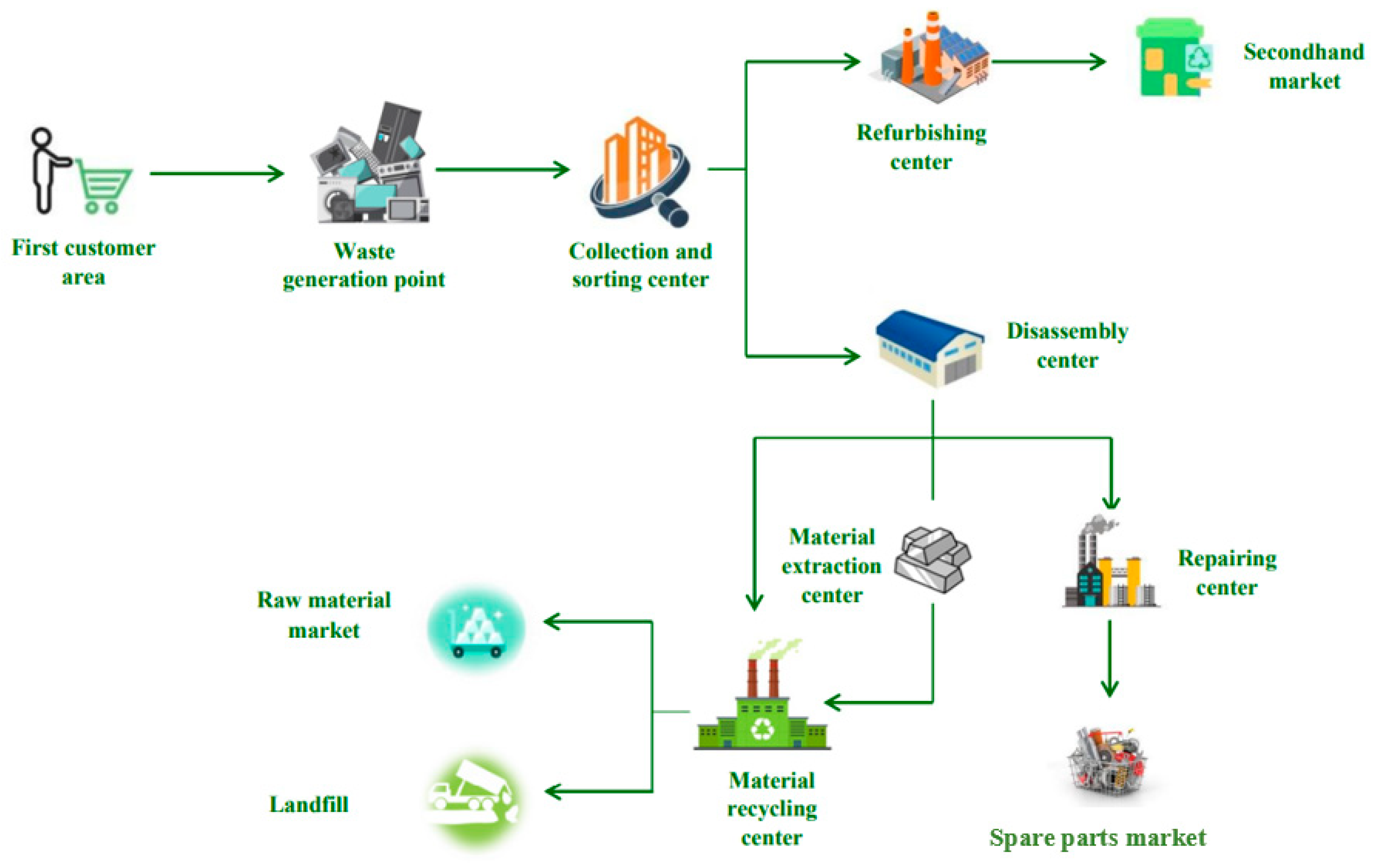
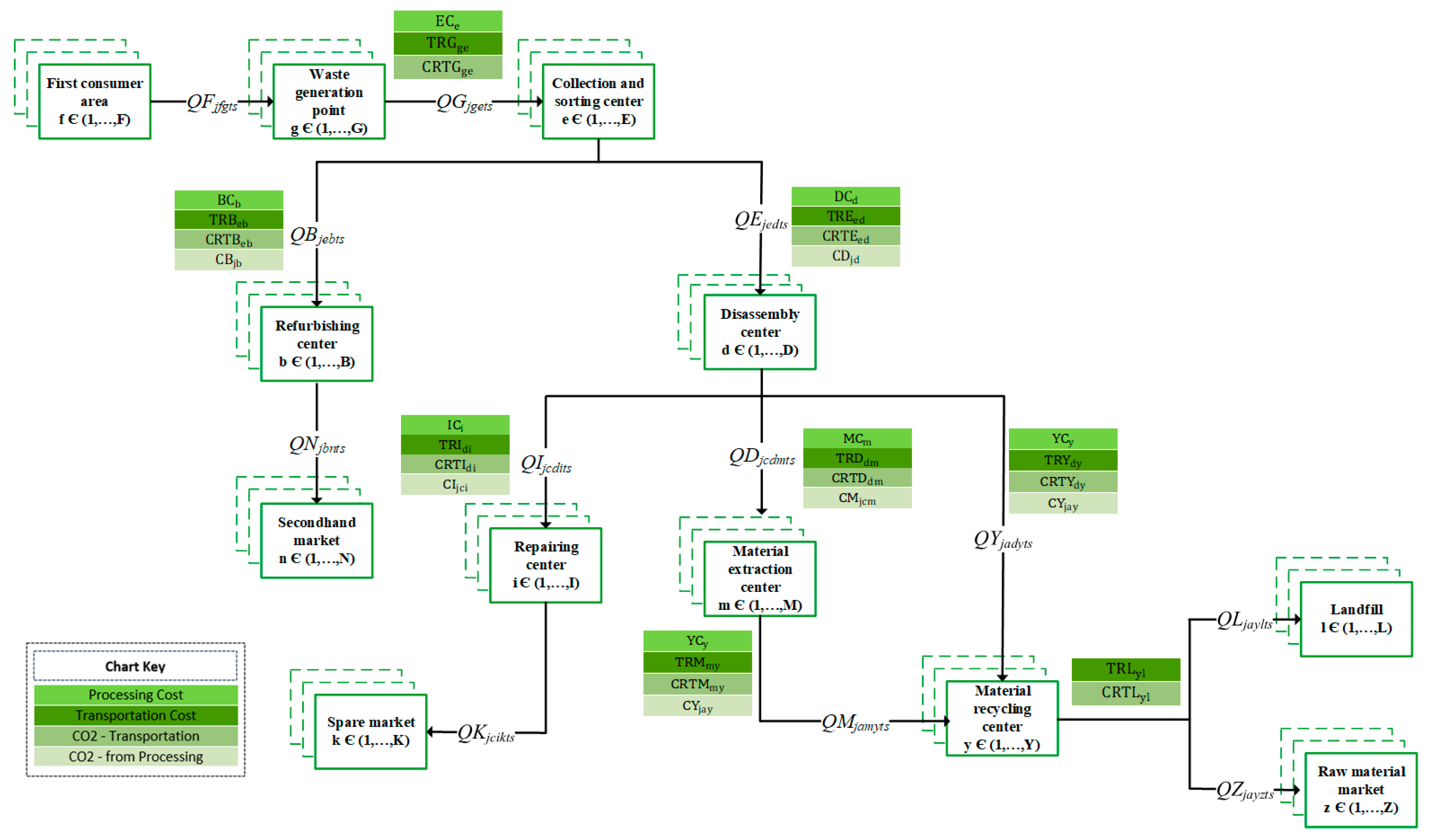

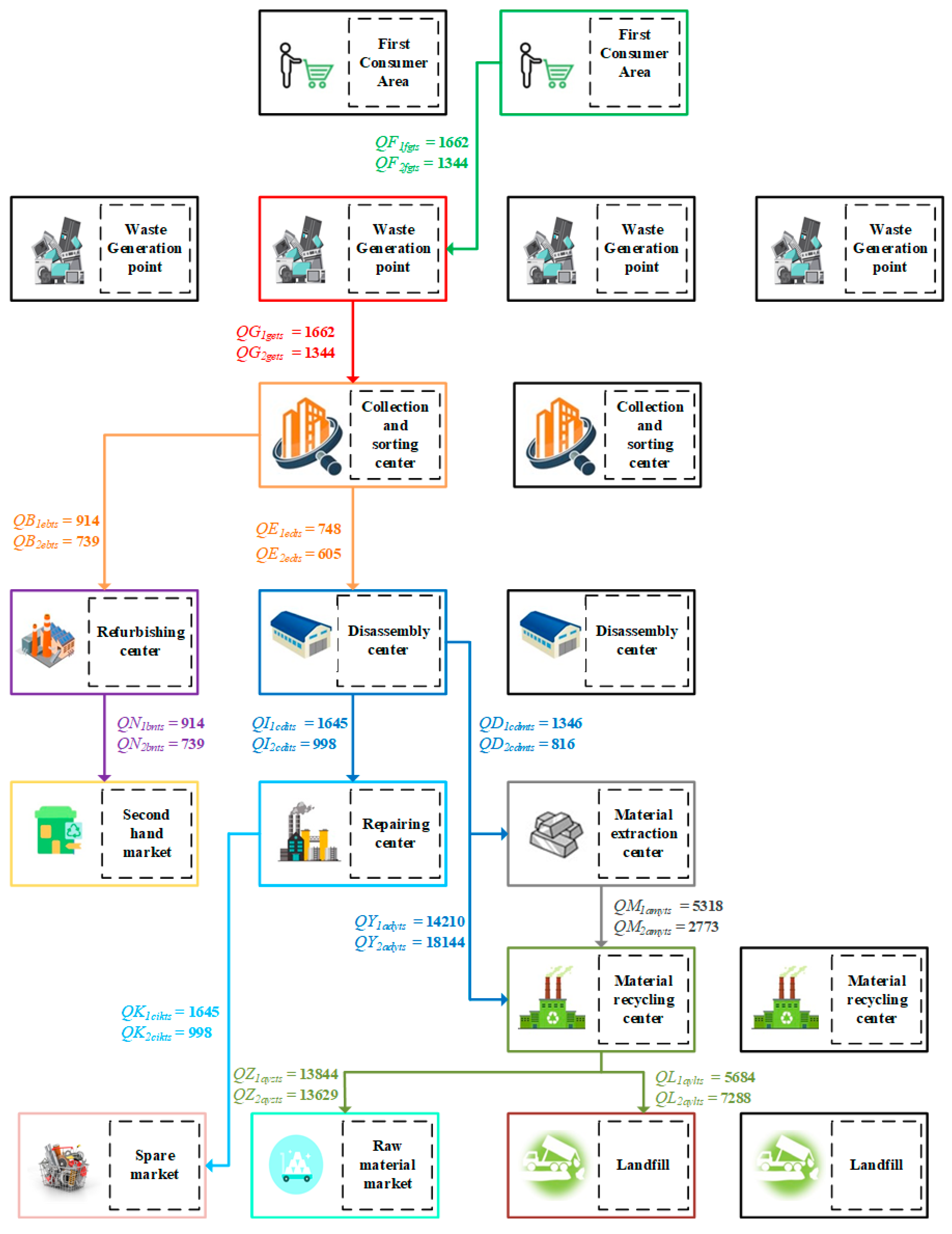
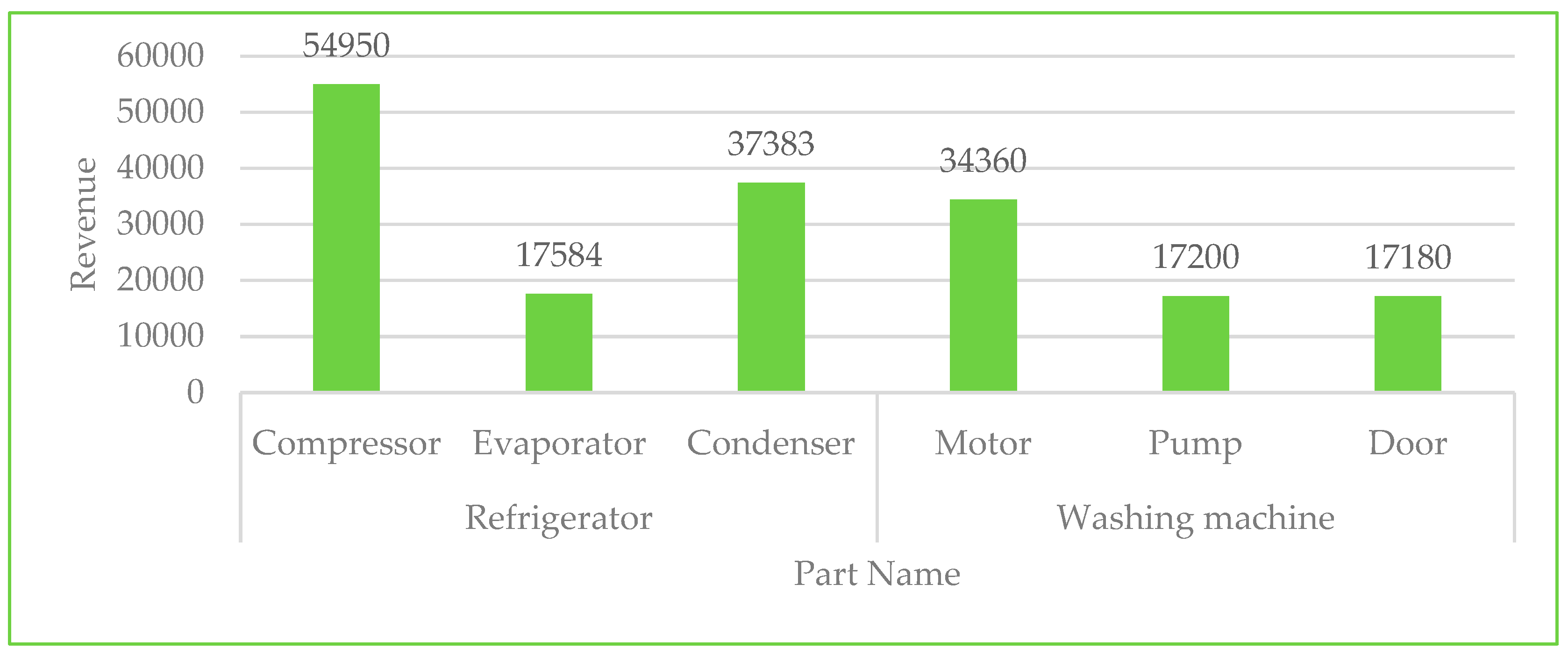
| Author Name | Paper Topic | Objective Function | Uncertainty | Multi-Product | Multi-Period | Multi-Objective | Mathematical Approach | ||||
|---|---|---|---|---|---|---|---|---|---|---|---|
| EN | EV | SL | Availability for Repair | Returns Quality | Returns Quantity | ||||||
| Ayvaz et al. [45] | Stochastic RSC design for e-waste | ✓ | ✓ | ✓ | ✓ | Two-stage stochastic programming | |||||
| Li et al. [7] | RSC for multi-products and multi periods | ✓ | ✓ | ✓ | ✓ | ✓ | Fuzzy integer non-linear programming | ||||
| Kuşakcı et al. [49] | RSC under fuzzy supply | ✓ | ✓ | Fuzzy programming approach | |||||||
| Yuchi et al. [50] | A bi-objective RSC under the emission trading scheme | ✓ | ✓ | ✓ | ✓ | Mixed-integer non-linear programming/genetic algorithm | |||||
| Tosarkani et al. [51] | A case-based robust possibilistic model for a multi-objective RSC | ✓ | ✓ | ✓ | ✓ | ✓ | ✓ | Scenario-based robust possibilistic, Two -phase fuzzy compromise approach | |||
| Doan et al. [18] | RSC under risk and uncertainty | ✓ | ✓ | ✓ | Fuzzy mixed-integer linear programming | ||||||
| Roudbari et al. [54] | RSC under uncertainty | ✓ | ✓ | ✓ | Two-stage stochastic mixed-integer programming | ||||||
| Karagoz et al. [56] | Stochastic RSC for vehicles | ✓ | ✓ | ✓ | Scenario-based stochastic optimization | ||||||
| This study | A stochastic multi-objective RSC | ✓ | ✓ | ✓ | ✓ | ✓ | ✓ | ✓ | ✓ | ✓ | Multi-stage stochastic programming |
| (a) Model indices. | |
| Notation | Description |
| f ∈{1,…,F} | Index of first consumer (s) |
| g ∈{1,…,G} | Index of waste generation points |
| e ∈{1,…,E} | Index of collection and sorting centers |
| b ∈{1,…,B} | Index of refurbishing centers |
| d ∈{1,…,D} | Index of disassembly centers |
| i ∈{1,…,I} | Index of repairing centers |
| m ∈{1,…,M} | Index of material extraction centers |
| y ∈{1,…,Y} | Index of material recycling centers |
| l ∈{1,…,L} | Index of landfills |
| n ∈{1,…,N} | Index of secondhand markets |
| z ∈{1,…,Z} | Index of raw material markets |
| k ∈{1,…,K} | Index of spare markets |
| s ∈{1,…,S} | Index of scenarios |
| t ∈{1,…,T} | Index of time periods |
| j ∈{1,…,J} | Index of product |
| Index of part | |
| Index of raw material | |
| Weight of raw material a in part c of product j | |
| Quantity of part c in product j | |
| Quantity of material a in product j | |
| Probability of scenario s | |
| Conversion ratio of material a in product j | |
| Percentage of product that can be refurbished or disassembled at time t under scenario s (quality of arrivals) | |
| Percentage of product that can be repaired at time t under scenario s (availability for repair) | |
| (b) Model parameters. | |
| Notation | Description |
| Fixed construction cost | |
| Fixed construction cost of the collection and sorting center e | |
| Fixed construction cost of refurbishing center b | |
| Fixed construction cost of dismantling center d | |
| Fixed construction cost of repairing center i | |
| Fixed construction cost of the material extraction center m | |
| Fixed construction cost of the material recycling center y | |
| Processing cost | |
| Collection and sorting cost per unit at the collection and sorting center e | |
| Refurbishing cost per unit at the refurbishing center b | |
| Disassembly cost per unit at the disassembly center d | |
| Repairing cost per unit at the repairing center i | |
| Extraction cost per unit at the material extraction center m | |
| Per Kg recycling cost at the material recycling center y | |
| Transportation cost | |
| Transportation cost per unit of product from the waste generation point g to the collection and sorting center e | |
| Transportation cost per unit of product from the collection and sorting center e to the refurbishing center b | |
| Transportation cost per unit of product from the collection and sorting center e to the disassembly center d | |
| Transportation cost per unit of repairable part from the disassembly center d to the repairing center i | |
| Transportation cost per unit of faulty part from disassembly center d to material extraction center m | |
| Per kg transportation cost of material from the material extraction center m to the material recycling center y | |
| Per kg transportation cost of material from the disassembly center d to the material recycling center y | |
| Per kg transportation cost of non-recyclable material from the material recycling center y to landfill l | |
| Selling price parameters | |
| Selling price of refurbished product j at the secondhand market n | |
| Selling price of repaired part c of product j at spare parts market k | |
| Selling price of recycled material a of product j at the raw material market z | |
| Capacity parameters | |
| Capacity of waste generation point g | |
| Capacity of the collection and sorting center e | |
| Capacity of refurbishing center b | |
| Capacity of disassembly center d | |
| Capacity of the repairing center i | |
| Capacity of the material extraction center m | |
| Capacity of the material recycling center y | |
| Capacity of landfill l | |
| Parameters for carbon emissions | |
| Processing | |
| Carbon emission from processing product j at the refurbishing center b | |
| Carbon emission from processing product j at the disassembly center d | |
| Carbon emission from the processing part c from product j at the repairing center i | |
| Carbon emission from the processing part c of product j at the material extraction center m | |
| Carbon emission from processing material a at material of product j at recycling center y | |
| Transportation | |
| Carbon emission from transportation of the product from the waste generation point g to the collection and sorting center e | |
| Carbon emission from transportation of product from the collection and sorting center e to the refurbishing center b | |
| Carbon emission from the transportation of products from the collection and sorting center e to the disassembly center d | |
| Carbon emission from transportation of parts from the disassembly center d to the repairing center i | |
| Carbon emission from the transportation of parts from the disassembly center d to the material extraction center m | |
| Carbon emission from the transportation of material from the material extraction center m to the material recycling center y | |
| Carbon emission from transportation of material from the disassembly center d to the material recycling center y | |
| Carbon emission from transportation of material from the material recycling center y to landfill l | |
| Social impact parameters | |
| Number of job opportunities created by establishing collection and sorting center e | |
| Number of job opportunities created by establishing refurbishing center b | |
| Number of job opportunities created by establishing disassembly center d | |
| Number of job opportunities created by establishing repairing center i | |
| Number of job opportunities created by establishing material extraction center m | |
| Number of job opportunities created by establishing material recycling center y | |
| Lost days due to work-related injuries during working at the collection and sorting center e while processing one unit of product j | |
| Lost days due to work-related injuries while working at the refurbishing center b while processing one unit of product j | |
| Lost days due to work-related injuries while working at the disassembly center d to process one unit of product j | |
| Lost days due to work-related injuries during working at the repair center i to process one unit of part c of product j | |
| Lost days due to work-related injuries while working at the material extraction center m while processing one unit of part c of product j | |
| Lost days due to work-related injuries while working at the material recycling center y while processing kg of material a of product j | |
| (c) decision variables | |
| Notation | Description |
| Quantity decision variables | |
| Quantity of arrivals at time t under scenario s | |
| Amount of product j sent from first consumer area f to waste generation point g at time t under scenario s | |
| Quantity of end-of-life and end-of-use products that are sent from the waste generation point g to the collection and sorting center e at time t under scenario s | |
| Quantity of end-of-use products transferred from collection and sorting center e to refurbishing center b at time t under scenario s | |
| Quantity of end-of-life products transferred from the collection and sorting center e to the disassembly center d at time t under scenario s | |
| Quantity of repairable part c from product j transferred from disassembly center d to repairing center i at time t under scenario s | |
| Quantity of faulty part c from product j transferred from disassembly center d to material extraction center m at time t under scenario s | |
| Quantity of material a from product j transferred from disassembly center d to material recycling center y at time t under scenario s | |
| Quantity of material a from product j transferred from material extraction center m to material recycling center y at time t under scenario s | |
| Quantity of non-recyclable material a from product j transferred from material recycling center m to landfill l at time t under scenario s | |
| Quantity of refurbished product j transferred from refurbishing center b to secondhand market n at time t under scenario s | |
| Quantity of repaired part c from product j transferred from repairing center i to spare market k at time t under scenario s | |
| Quantity of recycled material a from product j transferred from material recycling center y to raw material market z at time t under scenario s | |
| Binary variables | |
| Binary variable equals 1 if the collection and sorting center e is opened at time t, and 0 otherwise | |
| Binary variable equals 1 if the refurbishing center b is opened at time t, and 0 otherwise | |
| Binary variable equals 1 if the disassembly center d is opened at time t, and 0 otherwise | |
| Binary variable equals 1 if the repairing center i is opened at time t, and 0 otherwise | |
| Binary variable equals 1 if material extraction center m is opened at time t, and 0 otherwise | |
| Binary variable equals 1 if the material recycling center y is opened at time t, and 0 otherwise | |
| Binary variable equals 1 if landfill l is opened at time t, and 0 otherwise | |
| Product Type | Weight (kg) | Price (USD) |
|---|---|---|
| Refrigerator | 87 | 200 |
| Washing machine | 65 | 173 |
| (a) Refrigerator (j = 1) | |||||
| Part name | Part index | Quantity of parts/materials in product | Raw Material | Weight of raw material in part (kg) | Price (USD) |
| Parts | |||||
| Compressor | = 1 | Steel Copper | 8 1 | 50 | |
| Evaporator | = 1 | Aluminum | 2 | 16 | |
| Condenser | = 2 | Steel | 4 | 17 | |
| Materials | |||||
| Metal sheets | 4 | Steel | - | - | |
| Connecting pipe | 4 | Copper | - | - | |
| Plastic parts | 10 | Plastic | - | - | |
| Electrical wires | 1 | Copper | - | - | |
| (b) Washing machine (j = 2) | |||||
| Part name | Part index | Quantity of parts/materials in product | Raw material | Weight of raw material in part (kg) | Price (USD) |
| Parts | |||||
| Motor | = 1 | Steel Copper | 3.6 3.4 | 40 | |
| Pump | = 1 | Steel Copper Plastic | 0.4 0.3 0.3 | 20 | |
| Door | = 1 | Glass | 3.0 | 20 | |
| Materials | |||||
| Metal sheets | 15 | Steel | - | - | |
| Electrical wires | 1 | Copper | - | - | |
| Plastic parts | 14 | Plastic | - | - | |
| (a) Refrigerator (j = 1). | ||||
| Raw material | Index of raw materials | Selling price per kg (JD) | Availability for recycling | Conversion ratio |
| Steel | 0.88 | 85% | 0.85 | |
| Copper | 5.28 | 100% | 1 | |
| Plastic | 1.00 | 30% | 0.30 | |
| Aluminum | 1.54 | 60% | 0.60 | |
| (b) Washing machine (j = 2). | ||||
| Raw material | Index of raw materials | Selling price per kg (JD) | Availability for recycling | Conversion ratio |
| Steel | 0.88 | 85% | 0.85 | |
| Copper | 5.28 | 100% | 1 | |
| Plastic | 1.00 | 30% | 0.30 | |
| Glass | 0.40 | 100% | 1 | |
| Waste generation point (s) | ||||
| Capacity (product/year) | ||||
| Refrigerator Washing machine | = 6000 | = 6500 | = 6500 | = 6500 |
| = 7000 | = 7500 | = 6000 | = 6350 | |
| Collection and sorting station (e) | ||||
| Fixed construction cost (USD) | = 90,000 | = 95,000 | ||
| Capacity (product/year) | = 6000 | = 6500 | Refrigerator | |
| = 6500 | = 7000 | Washing machine | ||
| Processing cost (USD/product) | = 0.12 | = 0.12 | ||
| Refurbishing station | Refrigerator | Washing machine | ||
| Fixed construction cost (USD) | 100 | 500 | ||
| Capacity | 1400 | 2000 | ||
| Processing cost (USD/product) | 2.1 | 2.1 | ||
| Disassembly station (d) | ||||
| Fixed construction cost (USD) | = 100,000 | = 95,000 | ||
| Capacity (product/year) | = 6200 | = 5400 | Refrigerator | |
| = 6000 | = 5500 | Washing machine | ||
| Processing cost (USD/product) | = 2.5 | = 2.5 | ||
| Repairing station | Refrigerator | Washing machine | ||
| Fixed construction cost (USD) | = 200,000 | |||
| Capacity (product/year) | 20,000 | 25,000 | ||
| 20,800 | 25,000 | |||
| 20,600 | 20,000 | |||
| Processing cost (USD/part) | = 1.2 | |||
| Material extraction station | Refrigerator | Washing machine | ||
| Fixed construction cost (USD) | = 188,000 | |||
| Capacity (kg/year) | 20,000 | 25,000 | ||
| 25,000 | 25,000 | |||
| 20,000 | 25,000 | |||
| Processing cost (USD/part) | = 0.15 | |||
| Material recycling station (y) | ||||
| Fixed construction cost (USD) | = 250,000 | = 250,000 | ||
| Capacity (kg/year) | = 30,000 | = 35,000 | Refrigerator | |
| = 45,000 | = 40,000 | |||
| = 30,000 | = 30,000 | |||
| = 30,000 | = 30,000 | |||
| = 40,000 | = 45,000 | Washing machine | ||
| = 50,000 | = 50,000 | |||
| = 35,000 | = 40,000 | |||
| = 35,000 | = 35,000 | |||
| Processing cost (USD/part) | = 1.2 | = 1.2 | ||
| Landfill (l) | ||||
| Capacity (Kg/year) | = 25,000 | 20,000 | Refrigerator | |
| = 20,000 | 25,000 | |||
| = 20,000 | 20,000 | |||
| = 20,000 | 20,000 | |||
| = 25,000 | 20,000 | Washing machine | ||
| = 20,000 | 25,000 | |||
| 20,000 | 20,000 | |||
| = 20,000 | 20,000 | |||
| g1 | g2 | g3 | g4 | b1 | e1 | e2 | d1 | d2 | m1 | y1 | y2 | |
|---|---|---|---|---|---|---|---|---|---|---|---|---|
| e1 | 0.46 | 0.31 | 0.01 | 0.07 | ||||||||
| e2 | 0.68 | 0.02 | 0.33 | 0.29 | ||||||||
| b1 | 0.03 | 0.28 | ||||||||||
| d1 | 0.001 | 0.32 | ||||||||||
| d2 | 0.29 | 0.04 | ||||||||||
| i1 | 0.01 | 0.28 | ||||||||||
| m1 | 0.05 | 0.24 | ||||||||||
| y1 | 0.05 | 0.22 | 0.23 | |||||||||
| y2 | 0.28 | 0.03 | 0.42 | |||||||||
| l1 | 0.46 | 0.64 | ||||||||||
| l2 | 0.23 | 0.03 |
| g1 | g2 | g3 | g4 | b1 | e1 | e2 | i1 | m1 | y1 | y2 | |
|---|---|---|---|---|---|---|---|---|---|---|---|
| e1 | 1.52 | 1.03 | 0.003 | 0.22 | 0.1 | ||||||
| e2 | 2.24 | 0.005 | 1.07 | 0.94 | 0.9 | ||||||
| b1 | 0.005 | 1.04 | 0.02 | 0.15 | |||||||
| d1 | 0.94 | 0.12 | 1.04 | 0.79 | 0.16 | 0.74 | |||||
| d2 | 0.95 | 0.11 | |||||||||
| y1 | 0.77 | ||||||||||
| y2 | 1.4 | ||||||||||
| l1 | 1.49 | 2.14 | |||||||||
| l2 | 0.78 | 0.10 |
| Description | Parameter | |
|---|---|---|
| CO2 emission from refurbishing one unit of product (kg/unit) for both products | = 0.05 | |
| CO2 emission from disassembling one unit of product (kg/unit) for both products | = 0.03 = 0.02 | |
| CO2 emission from repairing one unit of the part (kg/unit) for both products | 0.10 0.08 0.10 | |
| CO2 emission from processing one unit of part (kg/unit) for both products | 0.01 0.02 0.02 | |
| 0.02 0.02 0.02 | ||
| CO2 emission from recycling one Kg of material (kg/unit) for both products | 0.30 | 0.20 |
| 0.20 | 0.15 | |
| 0.20 | 0.15 | |
| 0.30 | 0.20 |
| Station | Number of Job Opportunities Created | Lost Days Due to Work-Related Injuries (Day/Product) |
|---|---|---|
| Collection and sorting station | 20 20 | 0.01 0.01 |
| Refurbishing station | 19 | 0.01 |
| Disassembly station | 20 20 | 0.01 0.01 |
| Repairing station | 30 | 0.020.020.02 |
| Material extraction station | 25 | 0.025 0.0250.025 |
| Material recycling station | 3035 | 0.020.02 0.02 0.02 0.020.02 0.02 0.02 |
| Random Variable | Mode | Value | Probability | |
|---|---|---|---|---|
| Quality of returns | Good conditions | 0.55 | 0.45 | |
| Bad conditions | 0.45 | 0.55 | ||
| Availability for repair | Repairable | 0.55 | 0.45 | |
| Faulty | 0.30 | 0.55 | ||
| Random variable | Distribution | Mean | Sigma | |
| Quantity of returns (return rate) | Normal distribution | 1700 | 30 | |
| 1300 | 30 | |||
| Decision Variable | Value | Decision Variable | Value | Decision Variable | Value | Decision Variable | Value |
|---|---|---|---|---|---|---|---|
| ZG(2,) | 1 | ZG(2,) | 1 | ZG(2, ) | 1 | ZG(2,) | 1 |
| ZE(1,) | 1 | ZE(1,) | 1 | ZE(1,) | 1 | ZE(1,) | 1 |
| ZB(1,) | 1 | ZB(1,) | 1 | ZB(1,) | 1 | ZB(1,) | 1 |
| ZD(2,) | 1 | ZD(2,) | 1 | ZD(2,) | 1 | ZD(2,) | 1 |
| ZI(1,) | 1 | ZI(1,) | 1 | ZI(1,) | 1 | ZI(1,) | 1 |
| ZM(1,) | 1 | ZM(1,) | 1 | ZM(1,) | 1 | ZM(1,) | 1 |
| ZY(2,) | 1 | ZY(2,) | 1 | ZY(2,) | 1 | ZY(2,) | 1 |
| ZL(2,) | 1 | ZL(2,) | 1 | ZL(2,) | 1 | ZL(2,) | 1 |
| Scenario Number | Economic | Environmental Impact | Social Impact |
|---|---|---|---|
| Profit (USD) | Carbon Emissions (KgCO2) | ||
| 1 | 388,277 | 157,227.92 | 214 |
| 2 | 499,361 | 142,309.72 | 241 |
| ⁝ | ⁝ | ⁝ | ⁝ |
| 7 | 304,670 | 157,692.42 | 197 |
| 8 | 415,754 | 142,724.22 | 224 |
| 9 | 436,666 | 157,447.46 | 222 |
| 10 | 547,750 | 142,479.26 | 249 |
| 11 | 400,663 | 158,142.91 | 212 |
| ⁝ | ⁝ | ⁝ | ⁝ |
| 15 | 353,059 | 157,861.96 | 205 |
| 16 | 464,144 | 142,893.66 | 231 |
| Time | |||||||||||||||
| ∑ | ∑ | ||||||||||||||
| 1710 (1692) | 1710 (1692) | 1710 (1692) | 941 (761) | 941 (761) | 770 (931) | 462 (1024) | 231 (512) | 231 (512) | 923 (2047) | 923 (2047) | 1077 (838) | 539 (419) | 539 (419) | 2155 (1675) | |
| 1688 (1724) | 1688 (1724) | 1688 (1724) | 928 (776) | 928 (776) | 760 (948) | 456 (1043) | 228 (522) | 228 (522) | 912 (2086) | 912 (2086) | 1063 (853) | 532 (427) | 532 (427) | 2127 (1707) | |
| 1696 (1728) | 1696 (1728) | 1696 (1728) | 933 (778) | 933 (778) | 763 (950) | 458 (1045) | 229 (523) | 229 (523) | 916 (2091) | 916 (2091) | 1068 (855) | 534 (428) | 534 (428) | 2137 (1711) | |
| 1662 (1712) | 1662 (1712) | 1662 (1712) | 914 (770) | 914 (770) | 748 (942) | 823 (565) | 411 (282) | 411 (282) | 1645 (1130) | 1645 (1130) | 673 (1318) | 337 (659) | 337 (659) | 1346 (2636) | |
| Time | |||||||||||||||
| ∑ | ∑ | ||||||||||||||
| 1287 (1313) | 1287 (1313) | 1287 (1313) | 708 (761) | 708 (761) | 579 (931) | 174 (397) | 174 (397) | 174 (397) | 521 (1192) | 521 (1192) | 405 (325) | 405 (325) | 405 (325) | 1216 (975) | |
| 1342 (1298) | 1342 (1298) | 1342 (1298) | 738 (776) | 738 (776) | 604 (984) | 181 (393) | 181 (393) | 181 (393) | 544 (1178) | 544 (1178) | 423 (321) | 423 (321) | 423 (321) | 1268 (964) | |
| 1275 (1320) | 1275 (1320) | 1275 (1320) | 701 (778) | 701 (778) | 574 (950) | 172 (399) | 172 (399) | 172 (399) | 516 (1198) | 516 (1198) | 402 (327) | 402 (327) | 402 (327) | 1205 (980) | |
| 1344 (1279) | 1344 (1279) | 1344 (1279) | 739 (770) | 739 (770) | 605 (942) | 333 (211) | 333 (211) | 333 (210) | 998 (633) | 998 (633) | 272 (492) | 272 (492) | 272 (492) | 816 (1477) | |
| Time | |||||||||||||||
| ∑ | ∑ | ∑ | |||||||||||||
| 646 (503) | - | 539 (419) | 7326 (5695) | 8511 (6617) | - | 7695 (9306) | 3848 (4653) | 3078 (3722) | 14,621 (17,681) | - | 5387 (6514) | - | 462 (558) | 5848 (7073) | |
| 638 (512) | - | 532 (427) | 7231 (5803) | 8401 (6742) | - | 7596 (9482) | 3798 (4741) | 3038 (3793) | 14,432 (18,016) | - | 5317 (6637) | - | 456 (569) | 5773 (7206) | |
| 641 (513) | - | 534 (428) | 7266 (5816) | 8441 (6757) | - | 7632 (9504) | 3816 (4752) | 3053 (3802) | 14,501 (18,058) | - | 5342 (6653) | - | 458 (570) | 5800 (7223) | |
| 404 (791) | - | 337 (659) | 4577 (8964) | 5318 (10,414) | - | 7479 (9416) | 3740 (4708) | 2992 (3766) | 14,210 (17,890) | - | 5235 (6591) | - | 449 (565) | 5684 (7156) | |
| Time | |||||||||||||||
| ∑ | ∑ | ∑ | |||||||||||||
| 1216 (975) | 36 (29) | 1500 (1202) | 1378 (1105) | 4131 (3311) | - | 8108 (10,110) | 579 (722) | 8687 (10,832) | 17,375 (21,665) | - | 5676 (7077) | - | 1303 (1625) | 6979 (8702) | |
| 1268 (964) | 38 (29) | 1564 (1189) | 1437 (1092) | 4308 (3274) | - | 8455 (9995) | 604 (714) | 9059 (10,709) | 18,117 (21,417) | - | 5918 (6996) | - | 1359 (1606) | 7277 (8602) | |
| 1205 (980) | 36 (29) | 1486 (1209) | 1366 (1111) | 4093 (3329) | - | 8033 (10,164) | 574 (726) | 8606 (10,890) | 17,213 (21,780) | - | 5623 (7115) | - | 1291 (1634) | 6914 (8748) | |
| 816 (1477) | 24 (44) | 1007 (1822) | 925 (1674) | 2773 (5018) | - | 8467 (9848) | 605 (703) | 9072 (10,552) | 18,144 (21,104) | - | 5927 (6894) | - | 1361 (1583) | 7288 (8477) | |
| Time | |||||||||||||||
| ∑ | ∑ | ||||||||||||||
| 646 (503) | 2309 (2792) | 4386 (5072) | 9942 (8859) | 17,283 (17,225) | 1216 (975) | 2469 (3062) | 2079 (1925) | 8763 (10,312) | 14,527 (16,274) | ||||||
| 638 (512) | 2279 (2845) | 4330 (5168) | 9814 (9027) | 17,061 (17,551) | 1268 (964) | 2574 (3027) | 2168 (1903) | 9137 (10,194) | 15,148 (16,088) | ||||||
| 641 (513) | 2290 (2851) | 4350 (5180) | 9861 (9048) | 17,141 (17,592) | 1205 (980) | 2446 (3079) | 2060 (1935) | 8681 (10,367) | 14,391 (16,361) | ||||||
| 404 (791) | 2244 (2825) | 4076 (5367) | 7120 (12,165) | 13,844 (21,148) | 816 (1477) | 2565 (2999) | 1612 (2525) | 8637 (10,643) | 13,629 (17,645) | ||||||
| Refrigerator | ||||||
| Part/Material | Period 1 | Period 2 | Period 3 | Period 4 | Revenues (USD) | |
| Quantity of parts (part/year) | Compressor | 231 (512) | 228 (522) | 229 (523) | 411 (282) | 54,950 (91,927) |
| Evaporator | 231 (512) | 228 (522) | 229 (523) | 411 (282) | 17,584 (29,417) | |
| Condenser | 462 (1024) | 456 (1043) | 458 (1045) | 823 (565) | 37,383 (62,510) | |
| Total | 924 (2048) | 912 (2087) | 916 (2091) | 1645 (1129) | 109,917 (183,854) | |
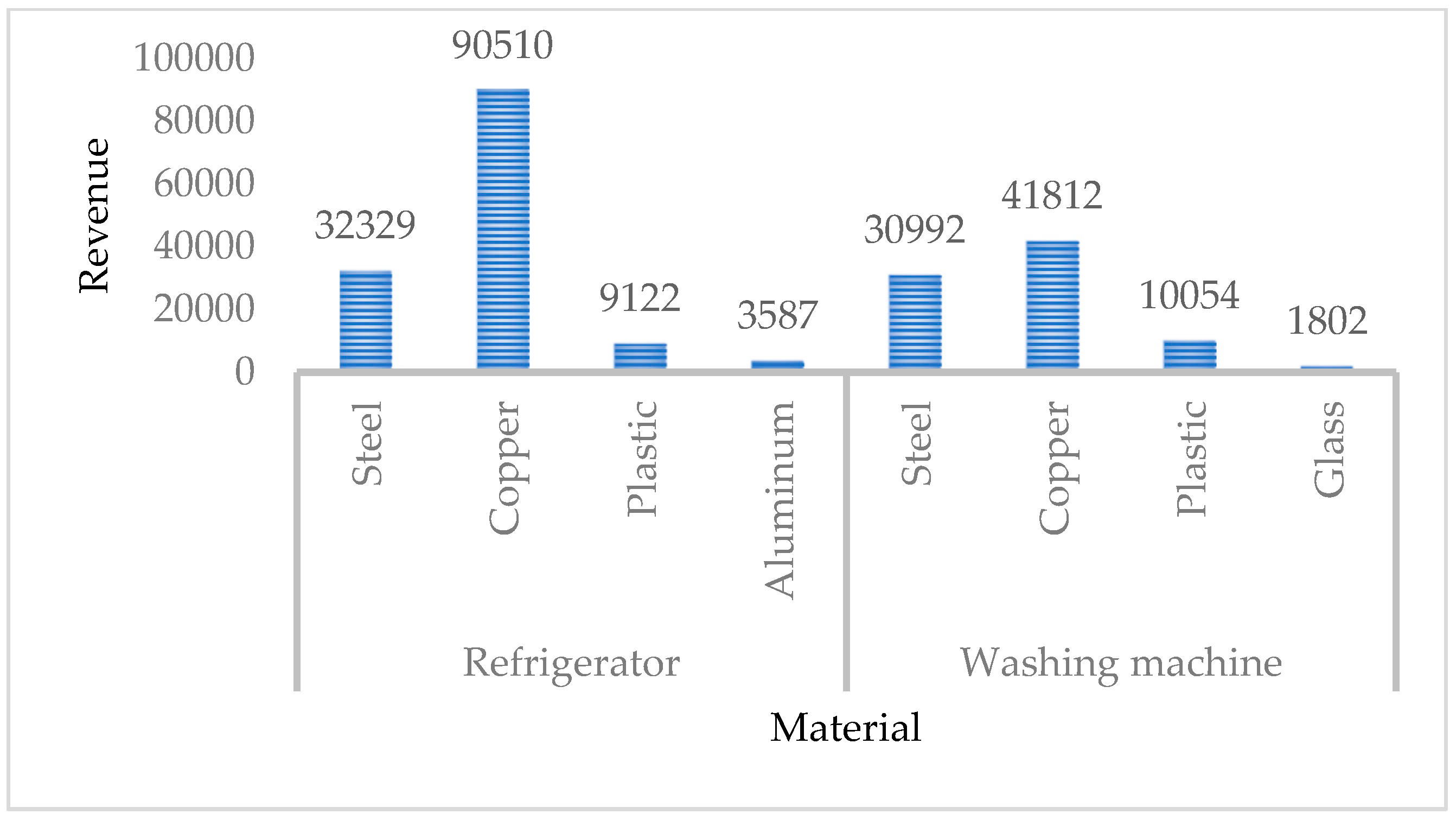
| Quantity of materials (kg/year) | Steel | 9942 (8859) | 9814 (9027) | 9861 (9048) | 7120 (12,165) | 32,329 (34,408) |
| Copper | 4386 (5072) | 4330 (5168) | 4350 (5180) | 4076 (5367) | 90,510 (109,751) | |
| Plastic | 2309 (2792) | 2279 (2845) | 2290 (2851) | 2244 (2852) | 9122 (11,312) | |
| Aluminum | 646 (503) | 638 (512) | 641 (513) | 404 (719) | 3587 (3571) | |
| Total | 17,283 (17,226) | 17,061 (17,552) | 17,142 (17,529) | 13,844 (21,148) | 135,547 (159,042) | |
| Washing machine | ||||||
| Part/Material | Period 1 | Period 2 | Period 3 | Period 4 | Revenues (USD) | |
| Quantity of parts (part/year) | Motor | 173 (397) | 181 (393) | 172 (399) | 333 (211) | 34,360 (56,007) |
| Pump | 174 (398) | 181 (393) | 172 (399) | 333 (211) | 17,200 (28,003) | |
| Door | 174 (398) | 181 (393) | 172 (399) | 332 (210) | 17,180 (27,983) | |
| Total | 521 (1193) | 543 (1178) | 516 (1198) | 998 (664) | 68,740 (111,993) | |
| Quantity of materials (kg/year) | Steel | 8763 (10,321) | 9137 (10,194) | 8681 (10,367) | 8637 (10,643) | 30,992 (36,535) |
| Copper | 2079 (1925) | 2168 (1903) | 2060 (1935) | 1612 (2525) | 41,812 (43,757) | |
| Plastic | 2469 (3062) | 2575 (3027) | 2446 (3079) | 2564 (2999) | 10,054 (12,167) | |
| Glass | 1216 (975) | 1268 (964) | 1204 (980) | 816 (1477) | 1,802 (1,758) | |
| Total | 14,527 (16,274) | 15,148 (16,088) | 14,391 (16,361) | 13,629 (17,645) | 84,660 (94,217) | |
| Scenario Number | Processing Cost (USD) | Transportation Cost (USD) | Construction Cost (USD) | Profit (USD) |
|---|---|---|---|---|
| 1 | 221,732 | 34,915 | 1,640,000 | 388,277 |
| 2 | 208,417 | 31,246 | 1,640,000 | 499,361 |
| ⁝ | ⁝ | ⁝ | ⁝ | ⁝ |
| 7 | 236,131 | 34,270 | 1,640,000 | 304,670 |
| 8 | 222,815 | 30,603 | 1,640,000 | 415,754 |
| 9 | 214,919 | 35,328 | 1,640,000 | 436,666 |
| 10 | 201,603 | 31,659 | 1,640,000 | 547,750 |
| ⁝ | ⁝ | ⁝ | ⁝ | ⁝ |
| 14 | 207,965 | 31,236 | 1,640,000 | 500,146 |
| 15 | 229,318 | 34,683 | 1,640,000 | 353,059 |
| 16 | 216,002 | 31,015 | 1,640,000 | 464,144 |
| Scenario Number | From Processing (kg CO2) | From Transportation (kg CO2) | Total Emissions (kg CO2) |
|---|---|---|---|
| 1 | 39,287.32 | 117,940.6 | 157,227.92 |
| 2 | 36,491.92 | 105,817.8 | 142,309.72 |
| ⁝ | ⁝ | ⁝ | ⁝ |
| 6 | 37,360.07 | 104,668.7 | 142,028.77 |
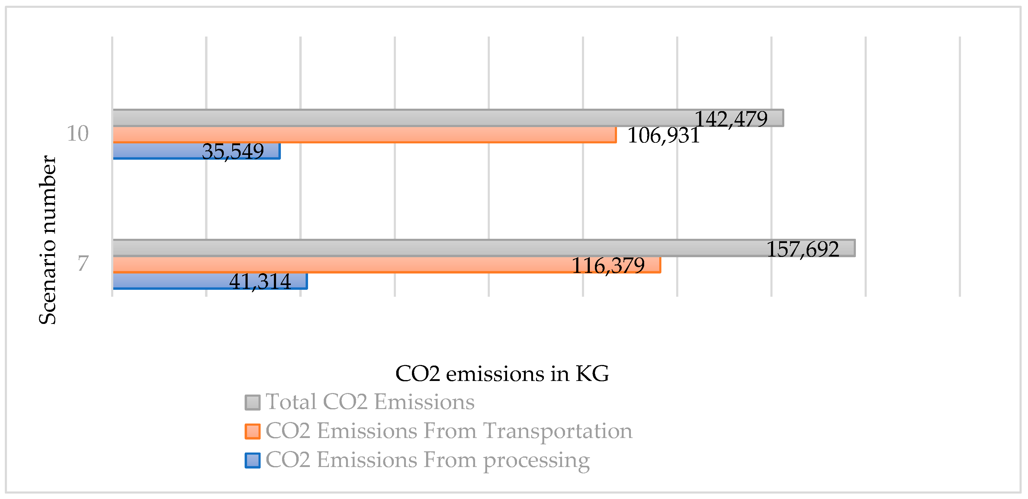
| 7 | 41,313.92 | 116,378.5 | 157,692.42 |
| 8 | 38,518.52 | 104,205.7 | 142,724.22 |
| 9 | 38,344.16 | 119,103.3 | 157,447.46 |
| 10 | 35,548.76 | 106,930.5 | 142,479.26 |
| ⁝ | ⁝ | ⁝ | ⁝ |
| 15 | 40,370.76 | 117,491.2 | 157,861.96 |
| 16 | 37,575.36 | 105,318.3 | 142,893.66 |
| Stage | T | CO2 Source (kg CO2) | Stage | T | CO2 Source (kg CO2) | Stage | T | CO2 Source (kg CO2) | Stage | T | CO2 Source (kg CO2) |
|---|---|---|---|---|---|---|---|---|---|---|---|
| Collection and sorting station | Processing | Disassembly station | Processing | Material extraction station | Processing | Landfill | Processing | ||||
| - | 40.46 (604.83) | 62.0 (48.8) | - | ||||||||
| - | 40.91 (609.23) | 62.6 (49.1) | - | ||||||||
| - | 40.11 (620.99) | 61.5 (49.5) | - | ||||||||
| - | 40.58 (596.13) | 39.9 (75.7) | - | ||||||||
| Transportation | Transportation | Transportation | Transportation | ||||||||
| 3086.9 (3095.2) | 1267.7 (1553.6) | 2662.9 (2093.5) | 1282.7 (1577.4) | ||||||||
| 3120.9 (3112.7) | 1281.7 (1562.4) | 2682.1 (2109.7) | 1305.0 (1580.9) | ||||||||
| 3060.1 (3139.4) | 1256.7 (1575.8) | 2640.0 (2125.7) | 1271.4 (1597.1) | ||||||||
| 3096.2 (3080.7) | 1271.5 (1546.3) | 1708.5 (3249.8) | 1297.2 (1563.3) | ||||||||
| Refurbishing station | Processing | Repairing station | Processing | Material recycling station | Processing | ||||||
| 82.4 (67.6) | 136.4 (305.7) | 6253.8 (7143.2) | |||||||||
| 83.3 (68.0) | 137.3 (308.1) | 6353.5 (7153.6) | |||||||||
| 81.7 (68.6) | 135.2 (310.4) | 6206.2 (7223.8) | |||||||||
| 82.7 (67.3) | 249.5 (166.4) | 6322.5 (7078.6) | |||||||||
| Transportation | Transportation | Transportation | |||||||||
| 164.8 (135.2) | 1502.4 (3368.4) | 18,271.0 (15,295.3) | |||||||||
| 166.7 (136.0) | 1513.2 (3394.5) | 18,425.9 (15,427.1) | |||||||||
| 163.4 (137.2) | 1489.5 (3420.3) | 18,088.6 (15,571.2) | |||||||||
| 165.3 (134.6) | 2749.0 (1833.5) | 11,939.3 (22,961.9) |
| Scenario 10 | −20% | −10% | Initial | +10% | +20% | Δ | |
|---|---|---|---|---|---|---|---|
| Quantity of returns | 2397 | 2697 | 2997 | 3297 | 3597 |  | |
| 2430 | 2730 | 3030 | 3330 | 3630 | |||
| 2371 | 2671 | 2971 | 3271 | 3571 | |||
| 2406 | 2706 | 3006 | 3306 | 3606 | |||
| Total | 9604 | 10,804 | 12,004 | 13,204 | 14,404 | ||
| Profit | 109,735 | 328,743 | 547,750 | 766,757 | 985,764 |  | |
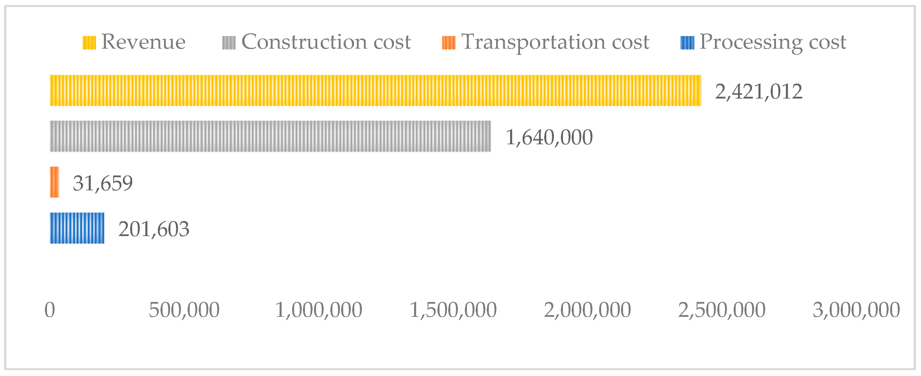
| Revenues | 1,936,387 | 2,178,700 | 2,421,012 | 2,663,325 | 2,905,637 | ||
| Processing cost | 161,327 | 181,465 | 201,603 | 221,741 | 241,880 | ||
| Transportation cost | 25,325 | 28,492 | 31,659 | 34,826 | 37,994 | ||
| Construction cost | 1,640,000 | 1,640,000 | 1,640,000 | 1,640,000 | 1,640,000 | ||
| Total cost | 1,826,652 | 1,849,957 | 1,873,263 | 1,896,568 | 1,919,873 | ||
| Environmental impact | 113,983 | 128,231 | 142,479 | 156,725 | 170,976 | ||
| Carbon emissions from processing | 28,445 | 31,997 | 35,549 | 39,100 | 42,652 | ||
| Carbon emissions from transportation | 85,537 | 96,234 | 106,931 | 117,627 | 128,324 | ||
| Social impact | 317 | 283 | 249 | 214 | 179 | ||
| Scenario 10 | −20% | −10% | Initial | +10% | +20% | Δ |
|---|---|---|---|---|---|---|
| Profit | 187,506 | 367,628 | 547,750 | 727,872 | 907,994 |  |
| Revenues | 2,114,091 | 2,267,552 | 2,421,012 | 2,574,473 | 2,727,934 | |
| Processing cost | 247,304 | 224,454 | 201,603 | 178,753 | 155,902 | |
| Transportation cost | 39,281 | 35,470 | 31,659 | 27,849 | 24,038 | |
| Construction cost | 1,640,000 | 1,640,000 | 1,640,000 | 1,640,000 | 1,640,000 | |
| Total cost | 1,926,585 | 1,899,924 | 1,873,263 | 1,846,601 | 1,819,940 | |
| Environmental impact | 176,859 | 159,669 | 142,479 | 125,290 | 108,100 | |
| CO2 emissions from processing | 44,092 | 39,820 | 35,549 | 31,277 | 27,006 | |
| CO2 emissions from transportation | 132,767 | 119,849 | 106,931 | 94,012 | 81,094 | |
| Social impact | 170 | 209 | 249 | 288 | 328 |
| Scenario 10 | −20% | −10% | Initial | +10% | +20% | Δ |
|---|---|---|---|---|---|---|
| Profit | 514,408 | 531,079 | 547,750 | 564,421 | 581,092 |  |
| Revenues | 2,393,569 | 2,407,291 | 2,421,012 | 2,434,734 | 2,448,455 | |
| Processing cost | 205,363 | 203,483 | 201,603 | 199,723 | 197,843 | |
| Transportation cost | 33,789 | 32,729 | 31,659 | 30,590 | 29,521 | |
| Construction cost | 1,640,000 | 1,640,000 | 1,640,000 | 1,640,000 | 1,640,000 | |
| Total cost | 1,879,161 | 1,876,212 | 1,873,263 | 1,870,313 | 1,867,364 | |
| Environmental impact | 150,473 | 146,476 | 142,479 | 138,483 | 134,486 | |
| CO2 emissions from processing | 36,576 | 36,062 | 35,549 | 35,035 | 34,521 | |
| CO2 emissions from transportation | 113,897 | 110,414 | 106,931 | 103,447 | 99,964 | |
| Social impact | 238 | 243 | 249 | 254 | 259 |
| Scenario 10 | −20% | −10% | Initial | +10% | +20% | Δ |
|---|---|---|---|---|---|---|
| Profit | 209,345 | 345,536 | 547,750 | 749,962 | 952,175 |  |
| Revenues | 2,082,608 | 2,218,799 | 2,421,012 | 2,623,225 | 2,825,438 | |
| Processing cost | 201,603 | 201,603 | 201,603 | 201,603 | 201,603 | |
| Transportation cost | 31,659 | 31,659 | 31,659 | 31,659 | 31,659 | |
| Construction cost | 1,640,000 | 1,640,000 | 1,640,000 | 1,640,000 | 1,640,000 | |
| Total cost | 1,873,263 | 1,873,263 | 1,873,263 | 1,873,263 | 1,873,263 | |
| Environmental impact | 142,479 | 142,479 | 142,479 | 142,479 | 142,479 | |
| CO2 emissions from processing | 35,549 | 35,549 | 35,549 | 35,549 | 35,549 | |
| CO2 emissions from transportation | 106,931 | 106,931 | 106,931 | 106,931 | 106,931 | |
| Social impact | 249 | 249 | 249 | 249 | 249 |
| Scenario 10 | −20% | −10% | Initial | +10% | +20% | Δ |
|---|---|---|---|---|---|---|
| Profit | 512,014 | 529,882 | 547,750 | 565,617 | 583,485 |  |
| Revenues | 2,385,277 | 2,403,145 | 2,421,012 | 2,438,880 | 2,456,748 | |
| Processing cost | 201,603 | 201,603 | 201,603 | 201,603 | 201,603 | |
| Transportation cost | 31,659 | 31,659 | 31,659 | 31,659 | 31,659 | |
| Construction cost | 1,640,000 | 1,640,000 | 1,640,000 | 1,640,000 | 1,640,000 | |
| Total cost | 1,873,263 | 1,873,263 | 1,873,263 | 1,873,263 | 1,873,263 | |
| Environmental impact | 142,479 | 142,479 | 142,479 | 142,479 | 142,479 | |
| CO2 emissions from processing | 35,549 | 35,549 | 35,549 | 35,549 | 35,549 | |
| CO2 emissions from transportation | 106,931 | 106,931 | 106,931 | 106,931 | 106,931 | |
| Social impact | 249 | 249 | 249 | 249 | 249 |
Disclaimer/Publisher’s Note: The statements, opinions and data contained in all publications are solely those of the individual author(s) and contributor(s) and not of MDPI and/or the editor(s). MDPI and/or the editor(s) disclaim responsibility for any injury to people or property resulting from any ideas, methods, instructions or products referred to in the content. |
© 2025 by the authors. Licensee MDPI, Basel, Switzerland. This article is an open access article distributed under the terms and conditions of the Creative Commons Attribution (CC BY) license (https://creativecommons.org/licenses/by/4.0/).
Share and Cite
Al-Refaie, A.; Shabaneh, A.; Lepkova, N. A Stochastic Multi-Objective Model for Optimal Design of Electronic Waste Reverse Supply Chain. Sustainability 2025, 17, 10693. https://doi.org/10.3390/su172310693
Al-Refaie A, Shabaneh A, Lepkova N. A Stochastic Multi-Objective Model for Optimal Design of Electronic Waste Reverse Supply Chain. Sustainability. 2025; 17(23):10693. https://doi.org/10.3390/su172310693
Chicago/Turabian StyleAl-Refaie, Abbas, Aya Shabaneh, and Natalija Lepkova. 2025. "A Stochastic Multi-Objective Model for Optimal Design of Electronic Waste Reverse Supply Chain" Sustainability 17, no. 23: 10693. https://doi.org/10.3390/su172310693
APA StyleAl-Refaie, A., Shabaneh, A., & Lepkova, N. (2025). A Stochastic Multi-Objective Model for Optimal Design of Electronic Waste Reverse Supply Chain. Sustainability, 17(23), 10693. https://doi.org/10.3390/su172310693


