Development of a Cost Prediction Model for Design Changes: Case of Korean Apartment Housing Projects

Abstract

Apartment buildings are significantly popular among South Korean construction companies. However, design changes present a common yet challenging aspect, often leading to cost overruns. Traditional cost prediction methods, which primarily rely on numerical data, have a gap in fully capitalizing on the rich insights that textual descriptions of design changes offer. Addressing this gap, this research employs machine learning (ML) and natural language processing (NLP) techniques, analyzing a dataset of 35,194 instances of design changes from 517 projects by a major public real estate developer. The proposed models demonstrate acceptable performance, with R-square values ranging from 0.930 to 0.985, underscoring the potential of integrating structured and unstructured data for enhanced predictive analytics in construction project management. The predictor using Extreme Gradient Boosting (XGB) shows better predictive ability (R² = 0.930; MAE = 16.05; RMSE = 75.09) compared to the traditional Multilinear Regression (MLR) model (R² = 0.585; MAE = 43.85; RMSE = 101.41). For whole project cost changes predictions, the proposed models exhibit good predictive ability, both including price fluctuations (R² = 0.985; MAE = 605.1; RMSE = 1009.5) and excluding price fluctuations (R² = 0.982; MAE = 302.1; RMSE = 548.5). Additionally, a stacked model combining CatBoost and Support Vector Machine (SVM) algorithms was developed, showcasing the effective prediction of cost changes, with or without price fluctuations.

1. Introduction

In South Korea, apartment buildings significantly influence the construction market and the economy of the construction industry [1], with millions of units being built between 1968 and 2016 [2]. Despite being a key focus for construction companies, apartment projects often face issues with design and construction mistakes, leading to extra costs for redesigns and reconstructions [3]. The causes of design changes in these projects can vary, including factors like project size, client requirements, performance of participants, construction costs, and the complexity of the project [4]. Historically, the design procurement process in both the public and private sectors has followed a co-planned ordering method [3]. In this method, design errors and changes are common because designers, selected by clients, might not fully consider the buildability of their designs [5]. This oversight can result in risks that affect the construction phase, such as increased time, cost, and compromised quality [6]. However, the industry lacks a clear understanding of how these factors directly cause quality issues in new apartment constructions [3].

Moreover, traditional methods for predicting the cost impacts of design changes, especially for Korean apartment buildings, often rely on numerical data and statistics [7]. On the other hand, text mining and NLP have been extensively utilized for BIM-based cost estimation [8]; budgeting, and cost overrun estimation [9,10,11]; their application to improve the cost control process; financial statement analysis; and overhead, direct, and indirect calculations have not been widely pursued. This approach may overlook detailed insights from textual descriptions of design changes, which could provide valuable information for cost predictions. Therefore, there is a potential benefit for a new method that uses NLP to analyze textual data, aiming for more accurate cost predictions.

Further developing of the previous research by Kim, Lee, and Kim (2022) [3], this study aims to provide a better understanding of the factors affecting design changes and to offer a new model that can predict the financial impact of these changes, focusing on apartment construction projects in South Korea. By using advanced ML and NLP techniques, the research seeks to improve how design changes are managed in apartment construction projects, helping industry professionals and policymakers reduce risks and achieve better project outcomes. This research employed a detailed dataset from 517 apartment projects by a major public real estate developer, covering 35,194 instances of design changes.

Following this introduction, Section 2 reviews the relevant literature, emphasizing the causes of design changes and their impact on construction costs. Section 3 describes the methodology, detailing the data collection and the analytical techniques employed in this study. Section 4 presents the results and discussion, including model performance and implications of the findings. Finally, Section 5 concludes with a summary of the key findings, the study’s limitations, and suggestions for future research.

2. Literature Review

2.1. Evaluate Effect Due to Design Changes in Construction Projects

Design changes in construction projects frequently occur due to a variety of reasons: discrepancies between actual site conditions and initial plans, technological advancements, client requests, or errors and omissions in design documents. Reasons for these adjustments include unclear or incorrect plans, differences between the planned and actual site conditions, the emergence of more efficient construction technologies, or changes requested by the project’s financiers. These modifications are a significant factor behind cost overruns, alongside inaccurate cost estimations, poor planning, and the inflation of resources [12]. Often, mistakes and missing parts in the plans are not noticed until building starts, which can make things like cost, timing, and quality uncertain. Design changes in construction projects add complexity due to subjective team and owner processes, unavoidable objective factors, mismatches between the provided information and site conditions, and design quality issues. These changes can lead to increased uncertainty and risk, affecting the cost, schedule and quality of construction projects, making them more sensitive to changes compared to other industries [6]. Research shows that finishing on time, staying on budget, and keeping up the quality are key to a project’s success [13]. But changes in design can threaten these goals, especially the budget. Studies have indicated that alterations made during the construction phase often lead to substantial cost overruns to preserve the project’s timeline and quality standards [14]. Despite effective management practices, these changes can inflate costs by 5 to 20% of the total construction budget [4]. It is observed that 17.43% of budget fluctuations in Korean apartment construction projects are due to various factors, among which changes in design and specifications rank as the most influential [3].

Preventing factors such as failures in design, price variations of materials, inadequate project planning, project scope changes, and design changes is a significant contributor to a project’s success [9]. As a result, research has been conducted on design changes in construction projects to explore their causes and impacts, highlighting key aspects of design modifications. Kikwasi (2021) [15] conducted a correlation study to establish the cause–effect relationship of claims in construction projects, emphasizing the importance of understanding how causes are linked to effects. Similarly, Afelete and Jung (2021) [16] identified 16 causes of design changes in power projects in Ghana, highlighting changes in the scope or plan by the owner as the most common trigger for design alterations. Gharaibeh, Matarneh et al. (2020) [4] explored the factors leading to design changes in Jordanian construction projects, emphasizing the impacts on project cost, schedule, and quality. Moreover, the relationship and impact of design change reasons on construction projects have been a focal point in the research.

Understanding why design changes happen in construction projects is important to stop them before they occur, but evidently, design changes are inherent in the construction industry [3]. Furthermore, it is crucial to know how to handle these changes well to reduce their bad effects and make sure the project is successful [5]. Yet, the body of research that thoroughly evaluates the specific impact of each design change—considering project characteristics, causes, and subsequent actions—is sparse. Accurately forecasting cost increases resulting from design alterations is a critical component of an impact assessment [7]. This evaluation is vital for a comprehensive understanding of the financial implications of design changes, thus empowering managers to make informed decisions. Every design modification not only incurs costs related to the change itself but may also indirectly influence other budgetary aspects of the project. Therefore, this study aims to create models that can predict both the direct costs and the broader financial implications of design changes on a project’s total budget. This predicted result is beneficial for making informed decisions that help manage the budget effectively and ensure the project’s financial health.

2.2. Cost Predictions in Construction

Predicting construction costs accurately is crucial for a project’s success [17]. Various studies have demonstrated effective methods for this. For example, Juszczyk et al. (2018) [18] estimated sports fields costs using Artificial Neural Networks (ANNs). Koo et al. (2011) [19] improved the prediction accuracy by optimizing the parameters in a Case-Based Reasoning (CBR) model. Plebankiewicz (2018) [10] applied Multiple Regression Analysis (MRA) for construction cost forecasting, while Shin (2015) [1] explored Boosting Regression Trees for early building cost estimations. Alqahtani and Whyte (2013) [20] also used ANNs to refine cost estimates by identifying significant cost factors. Lastly, Fernando (2023) [21] demonstrated ANN applications in early cost estimations for concrete bridges, showing various techniques for infrastructure cost predictions. Drawing from the quantitative methods utilized in the previous study, four principal research categories were distilled in this study.

• First, linear regression is a commonly used method for predicting construction project costs. Several studies have demonstrated the effectiveness of linear regression models in this area. Alshamrani (2017) [22] created linear regression models to predict the costs of building traditional and green college buildings in North America. In a similar way, Magdum and Adamuthe (2017) [23] used linear regression and Artificial Neural Networks to forecast costs for different construction projects. Petruseva et al. (2017) [24] tested how accurately linear regression models could predict construction costs, showing that these models are useful for forecasting costs. Surenth et al. (2019) [25] and Ahmed and Ali (2020) [26] also developed linear regression models to estimate the costs of specific projects in Sri Lanka and road projects, respectively. All these studies found a straightforward relationship between cost predictors and various cost indices using linear models. However, they did not consider non-linear relationships, which might be necessary for analyzing different types of data.
• Historical series analysis stands out as a popular method for modeling and predicting various cost indices, particularly in the construction industry, where forecasting costs based on historical data trends is crucial. Ashuri and Lu (2010) [27] applied four traditional time series models to the Construction Cost Index and found that these models performed well in stable, long-term datasets but faltered with data that showed high volatility. Expanding beyond traditional methods, the causal approach in time series analysis examines the impact of different economic indicators on cost indices. This method was tested by Aydınlı (2022) [28], who assessed the effectiveness of time series analysis in predicting construction costs in Turkey, emphasizing its potential in identifying cost trends. Furthermore, Isikdag et al. (2023) [29] delved into forecasting construction material indices using “Autoregressive Integrated Moving Average” models and optimized neural networks, demonstrating improved accuracy in cost predictability. These studies illustrate the benefits of causal time series analysis in offering insights into the factors driving Cost Index changes, presenting a significant improvement over a simplistic linear model. Nonetheless, despite its advantages in understanding and predicting cost dynamics, the causal time series method, much like its univariate counterparts, is primarily effective for short-term forecasting and may struggle with predicting large, sudden changes in the data.
• Third, ML algorithms offer a sophisticated approach to cost prediction, distinguishing themselves by learning from input data to make informed predictions about future costs. Unlike traditional static models, such as those used in time series analysis, ML algorithms adapt to data patterns to forecast outcomes more accurately [30]. For instance, Fan and Sharma (2021) [31] achieved a prediction accuracy within a 7% error margin using Support Vector Machine (SVM) and Least Squares SVM. Similarly, Meharie et al. (2021) [32] found that stacking ensemble ML algorithms surpassed traditional approaches like linear regression and neural networks in accuracy for highway construction cost predictions. Moreover, the research by Hsu et al. (2021) [33] and Ahn et al. (2017) [34] highlighted ML’s capability in forecasting various aspects of project performance and logistics costs. Cheng and Hoang (2014) [35] further demonstrated the use of LS-SVM for interval estimations in construction costs, underlining ML’s versatility in different predictive scenarios. Nonetheless, these successful applications underscore the dependence of ML models on the quality and structure of the data they are trained on, which could limit their effectiveness across different types of cost indices. Hashemi et al. (2020) [36] pointed out that the accuracy of ML-based cost forecasting is significantly influenced by the size and quality of the dataset, highlighting data availability and quality as potential challenges in applying ML techniques effectively in construction cost estimations.

2.3. Potential for Cost Increases Predictions of Design Changes

In the context of predicting cost increases due to design changes, combining prediction models entails analyzing both numerical and textual data from design change reports. Based on the advantages and disadvantages of each method discussed, method selection depends on what data source is available. NLP and ML could be considered as potential approaches. For instance, Lee and Yi (2017) [13] demonstrated that integrating unstructured text data with structured numerical data using text mining techniques significantly improves the accuracy of risk prediction models. Sharma et al. (2021) [37] conducted a survey on the applications of artificial intelligence for project cost estimations in construction and geotechnical engineering, highlighting the use of AI models for accurate construction cost predictions based on both numerical and text inputs. This process begins with preprocessing: normalizing numerical data for uniformity and converting text into a machine-readable format through tokenization and vectorization methods like TF-IDF [13,17]. Feature engineering follows, creating variables that capture the essence of both data types. Predictive models such as Random Forest (RL) or neural networks are then applied, possibly integrating NLP techniques to extract deeper semantic meaning from text. This approach allows to accurately predict cost impacts, leveraging the strengths of both ML for structured data and NLP for unstructured text to uncover insights hidden within the design change documentation, thereby aiding in more effective regression processes based on design modifications information [17]. The next section will detail the process of identifying and developing models for this study.

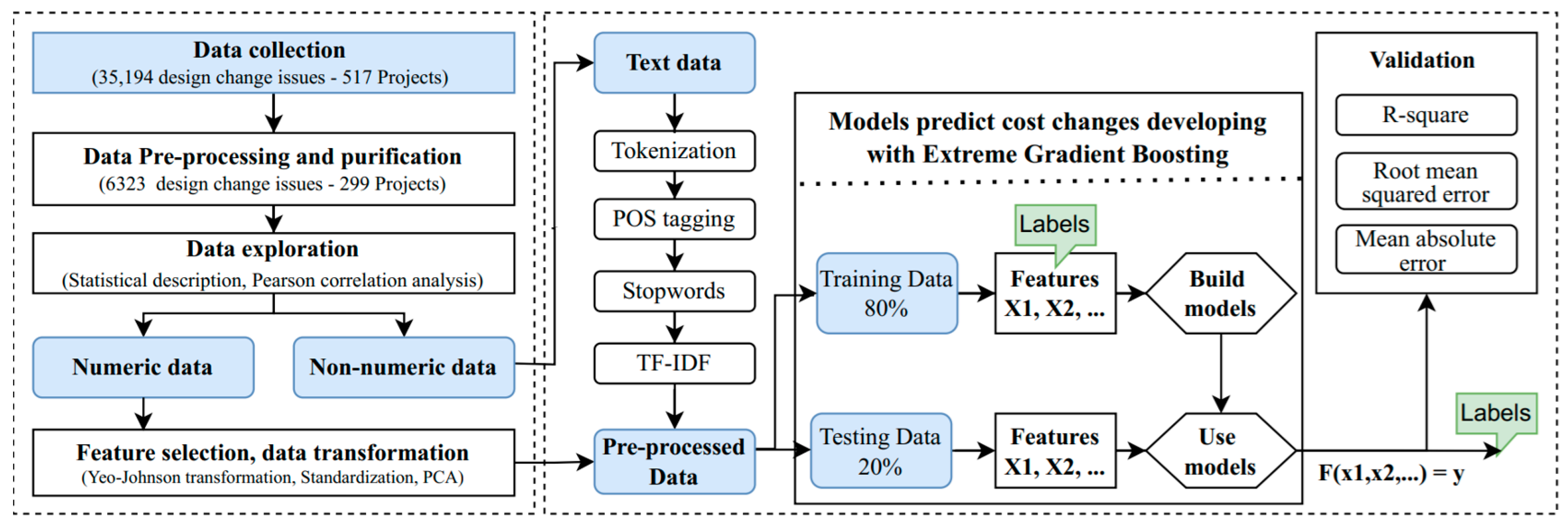
3. Data Collection and Preprocessing

The data used for this study indicate the design changes for a new apartment housing project conducted by a major public real estate developer in South Korea. The description of the original raw data is shown in

Table 1. Composition of the data on design changes.

ID	Contract Characteristic Indices	Description
X1	Number of Contractors	Total number of main contractors involved.
X2	Initial Contract Amount	Awarded bid price.
X3	Design Amount	Maximum budget allocated for design.
X4	Expected Amount	Estimated cost of the project.
X5	Name of Project	Includes developer’s information and project name.
X6	Regional	Encompasses South Korea’s 16 provinces.
X7	Project type	Construction purpose (Renovation, Sale, Rental, Self-use).
X8	Main Contractor	Lead contractor on the project.
X9	How to Determine the Successful Bidder	Criteria for contractor selection (Eligibility, Lowest Bid, etc.).
X10	Type (Construction Category)	Disciplines with design changes (e.g., Architectural, Structural).
X11	Adjustment Factors (Reasons)	Main reasons for design changes (e.g., Design Change, Government Request).
X12	Subcategory	Specific reasons for design alterations.
X13	Part/Object	Elements subject to design changes (e.g., Toilets, Windows).
X14	Detail	Detailed description of the design modifications.
X15	Contractor’s Explanation	Detailed rationale for the changes.
X16	Project Owner	Investing organization’s name.
X17	Contract End Date	Contract finalization date.
X18	Planned Completion Date	Publicly announced planned completion date.
X19	Actual Completion Date	Actual date of completion.
Y1	Increase or Decrease by Factor	Recorded cost variance per design change.
Y2	Contract Change Amount (including price fluctuations)	Total adjustment to the contract value, accounting for both design changes and market price variations.
Y3	Contract Change Amount (excluding price fluctuations)	Net change in contract cost due to design changes, not influenced by market price variations.

. The data consist of 35,194 design change issues that occurred in a total of 517 projects. The table delineates variables pertinent to the management and evaluation of design modifications within residential construction ventures. The research delineates these variables into two principal categories. The initial category (considered as the input) comprises preexisting information antecedent to the commencement of design modification activities, which includes data on contractors, investors, the overarching financial allocation for the project, geographical specifics of the site, and so on. The second category (considered as the output) embodies the consequential data stemming from the design alterations, exemplified by the incremental costs attributed to design modifications and the total actualized expenditures of the project (with/without price fluctuations).

Table 1 encapsulates the dataset that has been refined for the development of regression models to predict cost adjustments in apartment construction projects. The dataset originates from an extensive compilation of 35,194 instances of design alterations. Through rigorous data preprocessing and purification, the dataset was narrowed down to 6323 pertinent design change records. In the initial data screening phase, records with incomplete attributes, such as contract names, main contractors, initial contract prices, completion dates, disciplines, reasons for design modifications, and detailed descriptions, were excluded. Subsequent refinement steps involved the elimination of duplicate entries and the correction or removal of records with invalid attribute data. The resulting structured dataset, as depicted in the table, provides stable input variables to be utilized in the construction of the regression models.

4. ML-NLP Based Cost Prediction Model for Design Changes

The research framework (Figure 1) depicted the process of this study for building the cost prediction model involves collecting raw data from design change issues across multiple projects. To understand the collected data, statistical analysis is conducted and presented in

Table 2. Statistical description of the variables.

ID	Data Type	Detail
		Mean	STD	Min	Max	Skewness
X1	Numeric	1.82	0.95	1	6	1.01
X2	Numeric	43.31 × 109	27.12 × 109	9.67 × 109	199.00 × 109	2.50
X3	Numeric	59.87 × 109	35.11 × 109	0.10 × 109	205.71 × 109	1.63
X4	Numeric	58.01 × 109	31.60 × 109	0.00	198.99 × 109	1.47
X5	String	e.g., “Wonju Musil District 3 1BL Apartment Construction Section 4”
X6	Categorical	Seoul, Chungbuk, Chungnam, Gangwon, Gyeonggi, Gyeongbuk, Gyeongnam, Jeollabuk, Jeollanam, Jeju.
X7	Categorical	housing/redevelopment; rental; sale; sales + rental; self-operation.
X8	String	e.g., “Samneung Construction Co., Ltd., Gwangju-si, Republic of Korea”.
X9	Categorical	Eligible; Lowest price; Lowest price review; Qualification review success system; Qualification screening; Turnkey.
X10	Categorical	Architectural; Structural; Mechanical; Outdoor Mechanical; Electrical; Communication; Firefighting; Earthwork; District Earthwork; Building Earthwork; Landscape; and Common.
X11	Categorical	Design changes: changes mandated by the head office; alterations requested by government agencies; design errors; design improvements; site conditions; cost reductions; schedule extensions; changes in finishing materials; compliance with permit requirements; project plan modifications; additional construction; cost savings; civil complaints; sales promotions; settlement at completion; and other factors (17 in total).
X12	String	e.g., “Settlement Change in construction method, Civil complaints around the site”.
X13	Categorical	PIT floor; living room; stairwell; common area; common facilities; machine room; balcony; rooms; corridors; firefighting equipment; elevator; indoor piping; indoor wiring; rooftop; outdoor areas; outdoor piping; exterior walls; bathroom; electrical room; kitchen; main entrance; underground spaces; underground water tank; underground parking; piloti; entrance; among others.
X14	String	e.g., “Machine room size (2400 × 2700) Overhead height H = 4550 Machine room height H = 2300 Door installation 9 × 21SD Equipment loading window 12 × 15 AGW”
X15	String	e.g., “Application for residents planning Basic (file/history)”.
X16	String	e.g., “L.H.”
X17	Date	Dd/mm/yyyy
X18	Date	Dd/mm/yyyy
X19	Date	Dd/mm/yyyy
		Mean	STD	Min	Max	Skewness
Y1	Numeric	0.04 × 109	0.29 × 109	−3.80 × 109	10.86 × 109	16.01
Y2	Numeric	3.63 × 109	9.04 × 109	−45.94 × 109	24.96 × 109	−2.37
Y3	Numeric	2.50 × 109	4.07 × 109	−2.96 × 109	20.33 × 109	2.12

. The dataset includes several data types (e.g., numeric, string, date, and nominal). For numeric data, a Pearson correlation analysis and Yeo-Johnson transformation was conducted for feature selection and data transformation. For non-numeric data, a pine line of NLP techniques was conducted to process the data for prediction models. The NLP compasses the following steps:

• Tokenization to break the text into individual words.
• Parts-of-Speech tagging to assign grammatical labels to words in a sentence.
• Stop words to remove stop words from text data.
• TF-IDF vectorization converts a collection of documents into numerical representations based on the TF-IDF scores of terms.

The transformed numeric data and vectorized nonnumeric data were then concatenated into a preprocessed dataset. The dataset was partitioned into a training set (80%) and test set (20%). The training set is fed into the XGB model to predict the Y variable. The model is evaluated with R-square, root mean square error, and mean absolute error (MAE).

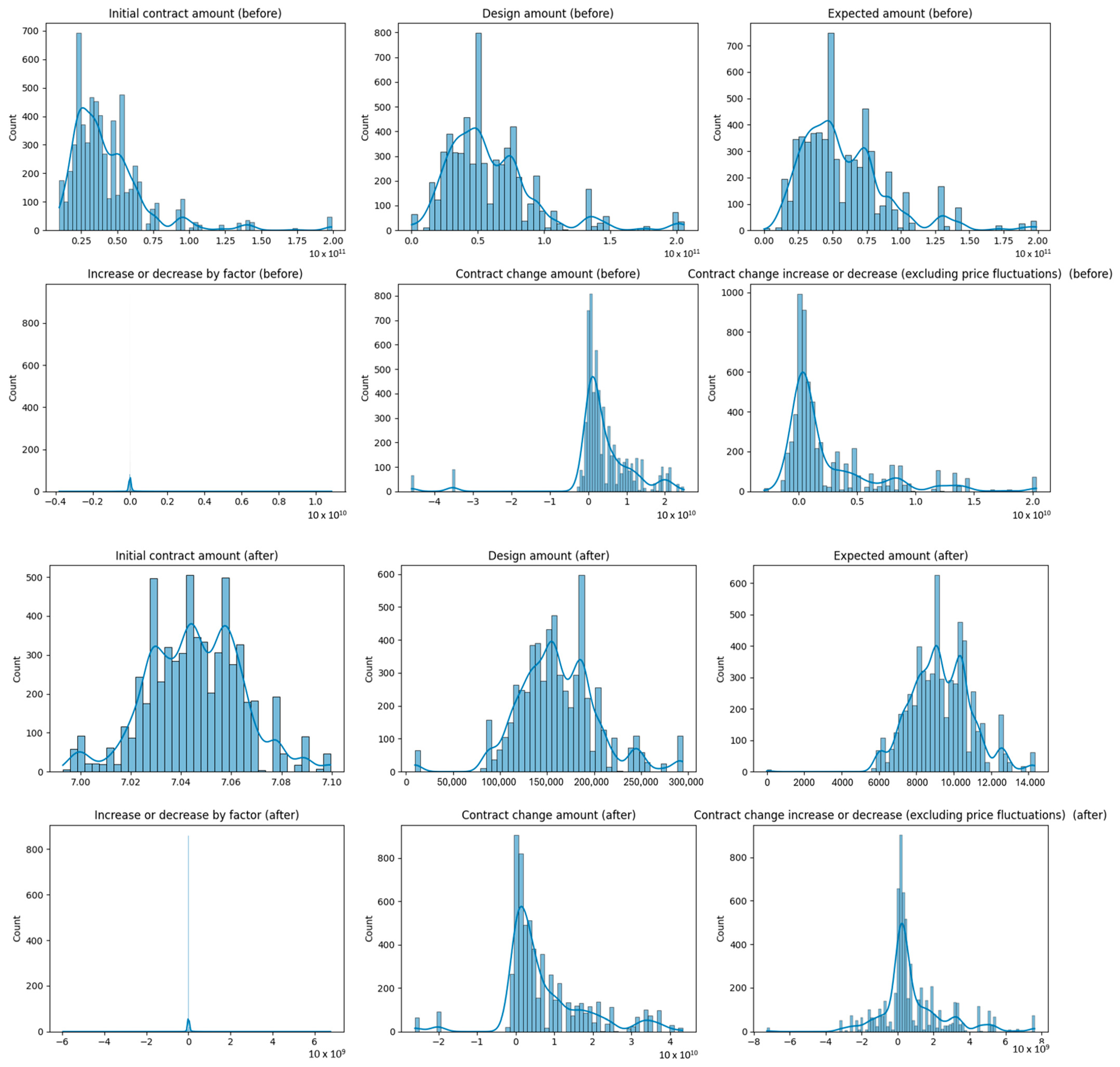
4.1. Data Description

The algorithms aim to forecast the cost increasing/decreasing of each design change reason and act, based on the information in the recorded design change reports outlined in Table 1. A dataset comprising 6116 samples from housing construction projects was gathered. This dataset comprises 15 discrete and 4 continuous independent variables, with 3 continuous variables serving as dependent variables. Table 2 presents a statistical description of the dataset. Regarding the numeric data, the minimum, maximum, and standard deviation values emphasize the extensive range of values for X2, X3, and X4, as well as Y1, Y2, and Y3. When there is a significant difference in the mean and variance of the variables, those with a large mean and variance have a greater impact on the other variables. As a result, important variables may be lost due to their low variation intervals. Additionally, this can impact the success of ML models [38]. The correlation heatmap illustrates (Figure 2) the relationships among several variables labeled X1 to X4 and Y1 to Y3. Notably, X1, X2, and X3 exhibit very strong positive correlations (0.85 to 0.93), suggesting they are closely related and possibly measure similar attributes. Among the Y variables, Y1 shows little correlation with the X variables and Y2, suggesting it operates independently. However, Y2 and Y3 have a moderate positive correlation of 0.54, pointing to some shared influence. The mentioned skewness and data distribution reveal that the data are positively skewed. Several statistical techniques and ML algorithms (such as linear regression and Gaussian Naive Bayes) have a strict assumption that the data in the training and test sets follow a normal or symmetric distribution [39]. Therefore, to guarantee the optimal model performance, it is necessary to apply a power transformation technique and normalization to this dataset. Moreover, Figure 3 reveals a significant correlation among variables X1, X2, and X3, suggesting a potential risk of multicollinearity.

For the non-numeric data, the variables can be viewed as categorical variables. However, data analysis reveals that each individual variable has more than 20 classes. This renders the handling of nominal variables ineffective. Therefore, this study employs NLP for all nonnumeric variables.

4.2. Data Processing

4.2.1. Yeo-Johnson Transformation

The Yeo-Johnson transformation is a versatile method used in various fields, including ML, statistics, and data analysis. This transformation allows for the normalization of data by applying a power transformation that can handle both positive and negative values. The studies by Walkowiak and Gniewkowski (2019) [40] and Bisandu et al. (2022) [41] highlighted the effectiveness of the Yeo-Johnson transformation in standardizing data and producing well-organized datasets that are easier to work with. Therefore, this study used Yeo-Johnson transformation to deal with the skewed data. Figure 3 shows the data distribution before and after transformation.

4.2.2. Data Standardization

Due to the disparate dimensions and varied physical interpretations of the collected data, the range of variations across the dataset is not uniform. Consequently, it is imperative to normalize the sample data before inputting it into the model. For numeric variables, normalization is achieved using StandardScaler, which scales the features to have a mean of 0 and a standard deviation of 1, ensuring that each feature contributes equally to the analysis [17].

4.2.3. Principal Component Analysis (PCA)

This study employs PCA to mitigate the issue of multicollinearity. PCA is an unsupervised technique used to reduce the dimensions of the datasets via singular value decomposition. It was first introduced by Karl Pearson and later independently developed by Hotelling. Jolliffe considered different forms of the procedure, and Jeffers and Chattopadhyay investigated several case studies of its applications [42].

The PCA procedure finds an orthogonal set of linear combinations of the variables in an n × m dataset X via a singular value decomposition. Suppose U Σ VT is the singular value decomposition of X, where the kth principal component of X is denoted by zk = Xvk, then Zk is the matrix of the first k principal components, i.e., Zk = XVk, where Vk contains the first k right singular vectors as columns of the matrix V = [V1, …, Vn], which is a matrix of size n × n, which columns are the normalized eigenvectors of XTX. PCR utilizes the resulting components of the data matrix XX by regressing the response Y onto Zk; that is, it fits the model Y = βZk + ε (Gwelo 2019) [43]. If the principal components are chosen correctly, this regression can overcome multicollinearity and lead to high accuracy prediction results [42]. The correlation between numeric input variables is shown in Figure 4.

4.2.4. Text Preprocessing Process

In this work, the process of text data processing begins with tokenization, where the raw text is broken down into smaller segments known as tokens, which may include both individual words and meaningful phrases [40]. This crucial step allows a natural language processing (NLP) system to assign a unique numerical ID to each token, facilitating further analysis. As NLP systems analyze these tokens, they learn to recognize patterns and respond accordingly. Subsequent to tokenization is Parts-of-Speech (POS) tagging, wherein each token is assigned a grammatical label, such as a noun, verb, or adjective, to delineate its function within a sentence, thereby enhancing the clarity and understanding of the text [13]. Following this, the process involves removing common stop words—words like “the”, “is”, and “at”, which are frequently used but carry minimal meaning—to sharpen the focus on more pertinent terms linked to specific topics like cost predictions in design changes. The final step involves applying the TF-IDF technique, which assesses the relevance of a word both within a single document and across a broader document corpus, highlighting terms uniquely significant to particular texts [11]. This method is beneficial in projects focused on predicting cost implications of design modifications in apartment housing, as it helps in prioritizing key terms and significantly boosts the accuracy and reliability of the predictive model.

4.3. Model Development and Evaluation

4.3.1. ML Models Developing

Model for Output 1 (OP1)—Increase or Decrease by Factor

This work employed algorithms for predicting OP1. The algorithms include XGB, RF, and Multilinear Regression (MLR).

• MLR

Regression analysis is a statistical technique utilized to establish the correlation between the dependent variable and the independent variables. More specifically, multiple linear regression investigates the connection between the dependent variable and several independent variables [44]. In this analysis, the dependent variable Y is a linear combination of multiple independent variables X. The objective is to minimize the sum of squared errors between the predicted and observed values of Y. The general equation for the multiple linear regression model is represented below as Equation (1):

Y = β0 + β1 + … + βnXn

(1)

where Y is the dependent variable; β0, β1, β2, β3, …, βn are known as regression weights or coefficients; and X1, X2, X3, …, Xn are independent variables or inputs.

In this study, the dependent variable Y is the “increase or decrease by factor”, and the independent variables X1, X2, X3, …, Xn are the inputs listed in Table 1.

• RF

RF is an ensemble learning technique that utilizes a sequence of regression decision trees for prediction purposes. In order to guarantee the independence of each tree, a random vector is selected from the input data and distributed evenly across the forest. The predictions of each tree within the forest are then combined by applying a combination of bootstrap aggregation and random feature selection [45].

The model’s hyperparameters are configured as follows: number of models = 100, tree depth = 20, and minimum node size = 1.

• XGB

XGB is a tree-based ensemble learning method proposed by Chen and Guestrin in 2016 [46]. The main difference between RF and XGB lies in their approach to tree creation. RF constructs trees individually, while XGB incorporates new trees to improve existing ones [47]. Gradient boosting enhances the flexibility of the boosting algorithm by combining multiple predictors from a group of weak learners, such as Classification and Regression Trees [47]. During the training phase, additive learning algorithms can be used for this process. After fitting the initial learner with all the input data, the residuals from the first model are used to correct the deficiencies in the performance of the weaker learner. This iterative fitting process continues until the stopping criterion is met.

The model’s hyperparameters are configured as follows: learning_rate = 0.3, number of models = 100, and tree depth = 20.

Model for Outputs 2 and 3 (OP2 and OP3)

The observation of a high correlation between the data in OP2 and OP3 with other numeric variables highlights the potential risk of multicollinearity. In response to this challenge, we adopt a multifaceted approach to pattern capture, leveraging both PCA and a stacked model comprising CatBoost and SVM. By combining the strengths of CatBoost, renowned for its prowess in handling categorical features, with the discriminative capabilities of SVM, our stacked model aims to enhance the predictive performance while mitigating the adverse effects of multicollinearity.

• CatBoost

In 2018, Dorogush et al. [48] introduced CatBoost, a novel gradient boosting method. CatBoost is notable for its balanced level-wise tree growth structures, which not only improve the training time efficiency but also address the issue of overfitting. In contrast to conventional boosting algorithms, CatBoost leverages the entire dataset during training by applying a random permutation to each example. Furthermore, it employs a unique approach to calculate leaf values when selecting the tree structure, effectively mitigating biased gradients.

• Stacked models

Stacking, a powerful ensemble technique, involves combining the predictions of multiple diverse models to enhance the overall performance. CatBoost, renowned for its robustness and effectiveness in handling categorical features, serves as the primary base learner in our stacked model. Leveraging its gradient boosting framework, CatBoost effectively captures intricate relationships within the data. Complementing CatBoost, this work integrated SVM, a classical ML algorithm known for its ability to delineate complex decision boundaries, particularly in high-dimensional spaces. By incorporating SVM alongside CatBoost in our stacked model, this study aims to capitalize on the respective strengths of both algorithms while mitigating their individual weaknesses.

The CatBoost model is configured with various hyperparameters, as delineated in

Table 3. Hyperparameters are set for the models.

Output	Hyperparameter
	Bagging_Temperature	Learning_Rate	Depth	l2_Leaf_Reg	Iterations
Contract change amount	0.7	0.3	10	5	500
Contract change increase or decrease	0.7	0.3	10	5	500

. Concurrently, the SVM model is equipped with the same selected hyperparameters, encompassing C = 40, epsilon = 0.9, and gamma = ‘scale’. This standardized approach facilitates comparative evaluations across models, allowing for a comprehensive assessment of the predictive performance under differing configurations.

4.3.2. Evaluation Metrics

This study targets regression analysis with continuous numerical outcomes—specifically, predicting cost impacts. To assess the precision of ML models, various performance criteria were considered. These included indicators such as the coefficient correlation coefficient (R), MAE, root mean square error (RMSE), and mean absolute percentage error (MAPE).

• R-square (R)

In statistics, R-square (R²) is a statistical measure that represents the proportion of the variance for a dependent variable that is explained by an independent variable or variables in a regression model.

$$R^2=1-\frac{{SS}_{res}}{{SS}_{tot}}$$

• ${SS}_{res}$ (Sum of Squares of Residuals) measures the variation of the observed data points from the fitted values.
• ${SS}_{tot}$ (Total Sum of Squares) quantifies the total variation in the dependent variable.

• Root mean squared error (RMSE)

RMSE is a widely used metric for evaluating the accuracy of predictive models, such as regression models. It quantifies how significant the usual differences are between predicted and observed values. In mathematical terms, the RMSE is calculated as follows:

$$\mathrm{R}\mathrm{M}\mathrm{S}\mathrm{E}=\sqrt{\frac{1}{N}{\sum }_{i=1}^N{\left(s_i-p_i\right)}^2}$$

• N is the number of observations or the total number of data points in the dataset.
• $s_i$ is the actual value for the ith observation.
• $p_i$ is the predicted value for the ith observation.

• MAE

MAE is a commonly used measurement for evaluating the precision of a predictive model, particularly in regression situations. It quantifies the average number of discrepancies between predicted and actual observed values. Mathematically, MAE is calculated as follows:

$$MAE=\frac{1}{n}{\sum }_{i=1}^n\left|s_i-p_i\right|$$

• n is the number of observations or the total number of data points in the dataset.
• $s_i$ is the actual value for the ith observation.
• $p_i$ is the predicted value for the ith observation.

5. Prediction Performance

5.1. Increase or Decrease by Factor

Table 4. Model performance in OP1.

Model	Dataset	R2	MAE	RMSE
XGB	train	0.955	14.149	67.7
	test	0.930	16.05	75.09
Multilinear Regression	train	0.476	66.11	238.14
	test	0.585	43.85	101.41

present the model performance of the XGB and MLR models. The RF model, despite grid search cross-validation optimization, achieved similar results to Multilinear Regression. Therefore, only the results of XGB and MLR are presented. For XGB, the model achieves high R² values of approximately 0.955 and 0.930 for the training and test sets, respectively. This indicates that a significant portion of the variance in the target variable (increase or decrease by factor) is explained by the predictors. The MAE and RMSE values for the test set (16.05 million won and 75.09 million won, respectively) signify that, on average, the model’s predictions deviate by approximately 16.05 million won from the actual values, with RMSE reflecting the dispersion of the prediction errors. The predicted values are visualized in Figure 5.

For MLR, the model achieved R² values at 0.476 and 0.585 for the training and test sets, respectively. Meanwhile, the MAE values are recorded at 66.11 and 43.85, with RMSE values of 238.14 and 101.41, for the training and test sets, respectively. These metrics collectively suggest that the model struggles to effectively capture the relationships among the variables. Upon closer examination of the accompanying figure, it becomes apparent that the range of independent input variables is notably extensive. Instances where the input values are excessively large or small correspond to greater disparities between the model’s predictions and the actual values. Moreover, a discernible disparity exists between the training and test sets in terms of data distribution. Specifically, the training set, spanning from 2007 to 2010, exhibits considerably larger fluctuations in values compared to the test set, which extends from 2010 to 2011. Consequently, the model demonstrates a relatively superior performance on the test set compared to the training set. In summary, the observed performance inadequacies in the MLR model underscore its limitations in effectively modeling the complex relationships inherent in the data. The disparities in performance between the training and test sets further emphasize the need for more sophisticated modeling techniques to better capture the intricacies of the dataset. The predicted values are visualized in Figure 6.

The superior performance of the XGB model compared to the MLR model can be attributed to several key factors:

Non-linearity: The dataset includes a diverse array of input features, ranging from numerical data to textual and temporal elements, which collectively contribute to the determination of the output. In this context, the intricate relationships among these heterogeneous input variables and the resultant output are characterized by non-linear dynamics. XGB is capable of capturing non-linear relationships between the independent and dependent variables more effectively than MLR. MLR assumes a linear relationship between the variables, whereas XGB can model complex, non-linear patterns in the data.

Robustness to Outliers: As illustrated in the dataset exploration phase, the target variable “increase or decrease by factor” exhibits a wide range of values with numerous outliers. Given its susceptibility to outliers and strict assumption of normality in data distribution, MLR is notably affected, thereby impinging upon the model performance when confronted with such data characteristics. Conversely, XGB demonstrates enhanced resilience to outliers within the dataset. The tree-based methodology employed by XGB facilitates the partitioning of data into smaller, more manageable subsets, thereby attenuating the influence of extreme values on the model predictions. Consequently, the pronounced robustness of XGB to outliers stands in stark contrast to MLR’s vulnerability, underscoring its superiority in scenarios characterized by data outliers and non-normally distributed data.

5.2. Contract Change Amount

Table 5. Model performance in OP2 and OP3.

Output (in Million Won)	Dataset	R2	MAE	RMSE
Contract change amount	train	0.994	422.3	701.8
	test	0.985	605.1	1009.5
Contract change amount (excluding price fluctuations)	train	0.9934	211.7	330.5
	test	0.982	302.1	548.5

and Figure 7 demonstrate that the stacked model successfully predicts OP2 and OP3 in both the train and test sets. Furthermore, it exhibits no issues with multicollinearity and is highly responsive to noise, and the model demonstrates exceptional predictive power, with R² values exceeding 0.99 for both the training and test sets. This indicates that the model explains nearly all of the variance in the contract change amount. The MAE and RMSE values for the test set (605.1 million won and 1009.5 million won, respectively) suggest slightly higher prediction errors compared to the “increase or decrease by factor” dataset, albeit still within reasonable bounds.

5.3. Contract Change Amount (Excluding Price Fluctuations)

In a similar vein as OP2, the stacked model also demonstrates acceptable prediction results in OP3. The correlation analysis reveals a strong correlation between OP2 and OP3, indicating that the model’s proficiency in predicting OP2 extends equally to OP3. The results in Table 5 exhibit a robust performance, with R-square values around 0.9934 for the training set and 0.982 for the test set. This indicates that the model accurately captures variations in the contract change amount, excluding price fluctuations. The MAE and RMSE values for the test set (302.1 million won and 548.5 million won, respectively) demonstrate the model’s ability to make predictions with relatively low error rates. The results on the training and test sets are visualized in Figure 8.

6. Limitations and Discussion

The models 10,000 developed in this study effectively predicted the cost changes (OP1), as well as the adjustments in contract amounts due to design changes, both with (OP2) and without (OP3) price fluctuations considered. The OP2 and OP3 predictions were particularly accurate, because they closely aligned with the patterns found in the numeric input data, facilitating easier and more accurate forecasts. The application of PCA (a method for data organization) and stacked models (combining different prediction techniques) improved the models’ performance across various scenarios and mitigated the problem of variables being too closely linked (multicollinearity). This adjustment also enhanced the models’ ability to handle outlier data. However, the story was different for OP1, where there was a very low correlation with the numeric inputs. This underscores the importance of carefully extracting information from non-numeric data and choosing an appropriate model that can effectively manage a mix of data types. Upon testing multiple models, it was found that the XGB model (an advanced decision tree algorithm) delivered the best prediction results.

Despite the advancements made in predicting cost changes due to design changes with reasonable accuracy, this study highlights significant areas for improvement. Future works should focus on expanding the data collection, optimizing the algorithms further, and refining the selection of features for the model.

• Firstly, the dataset, while extensive, is constrained to South Korean apartment projects. This project’s typical and geographical limitations may affect the generalizability of the findings to construction practices and market conditions in other regions. Future research could benefit from incorporating the data from a diverse set of locations to enhance the global applicability of the model.
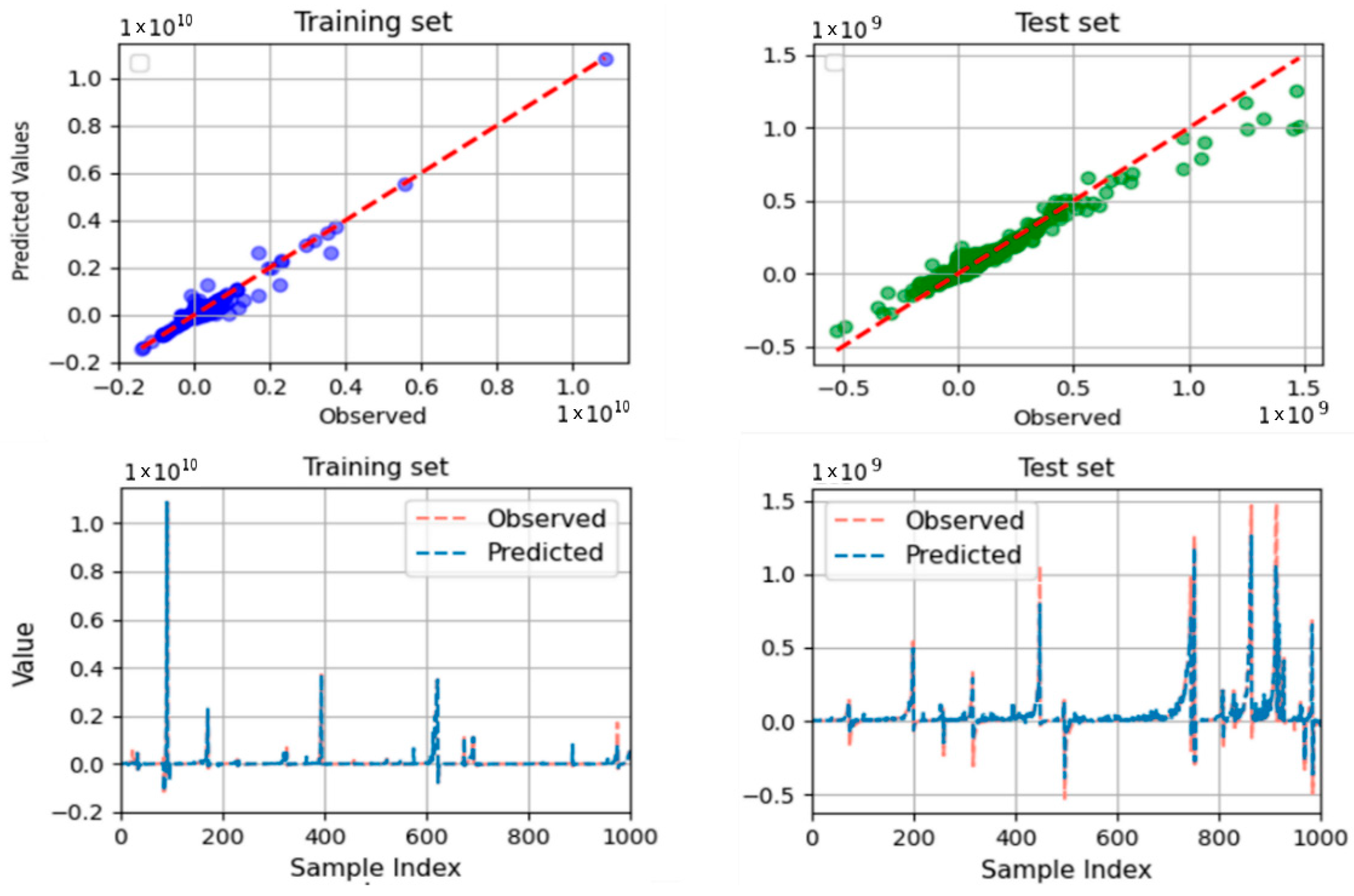
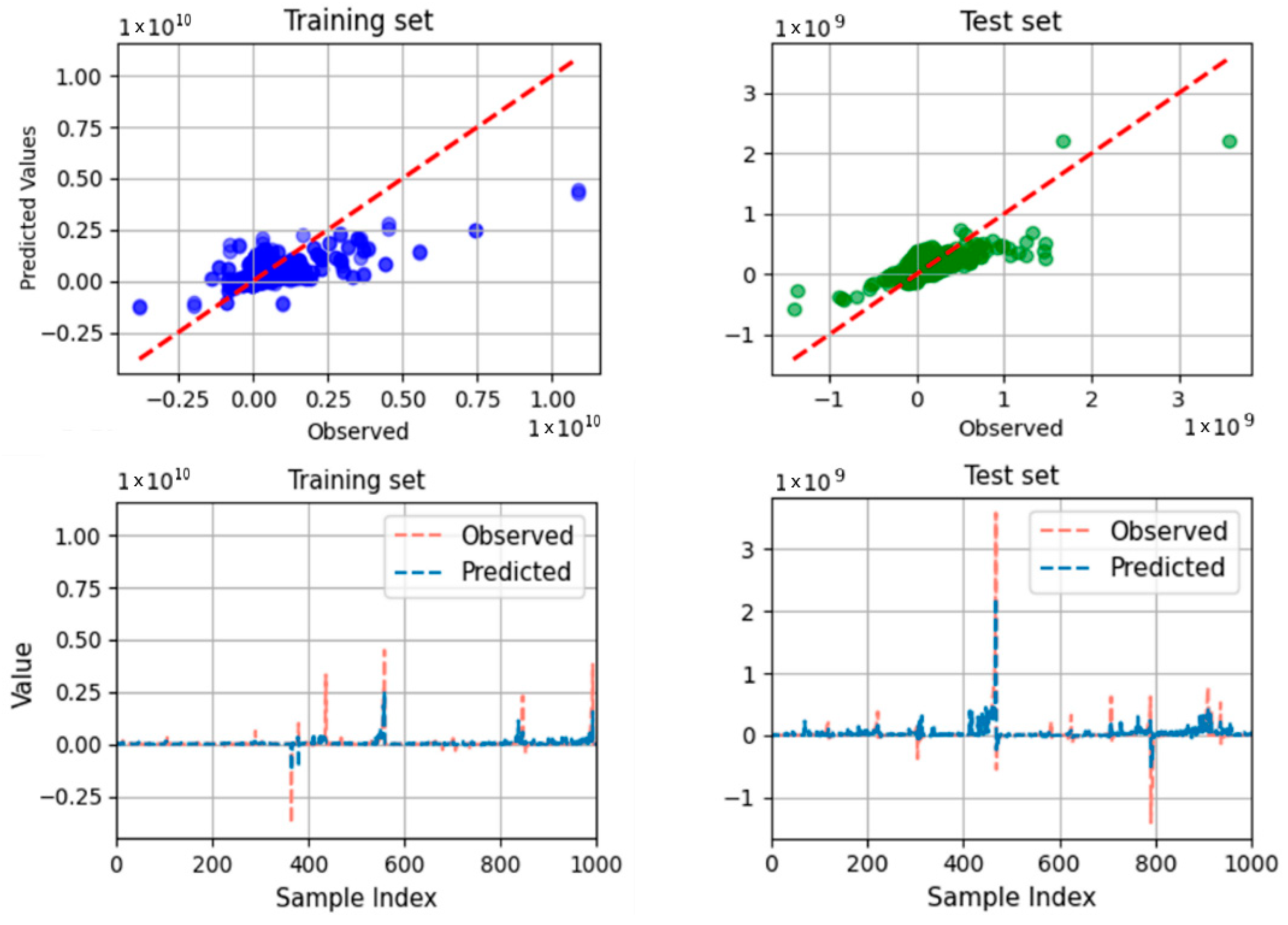
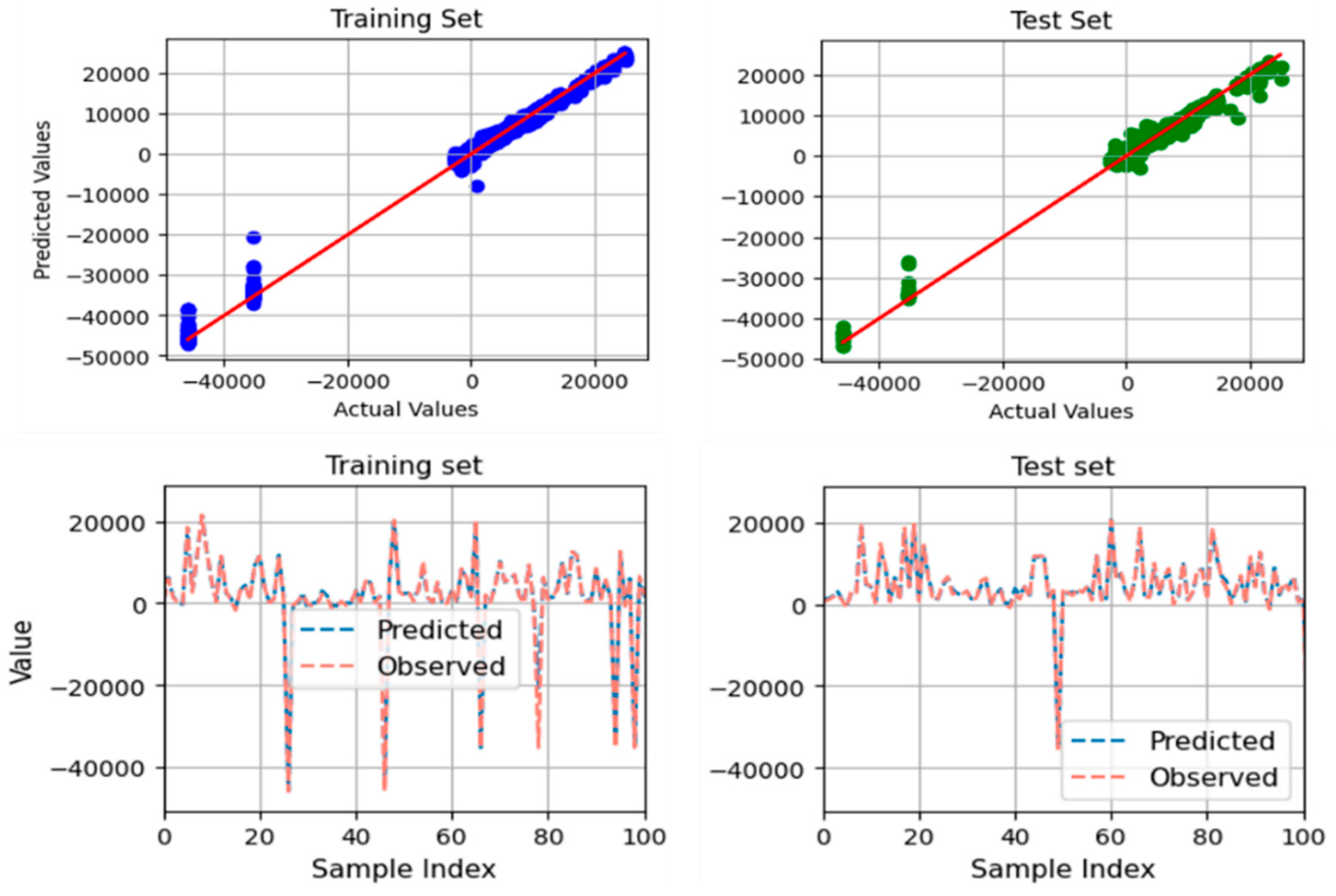
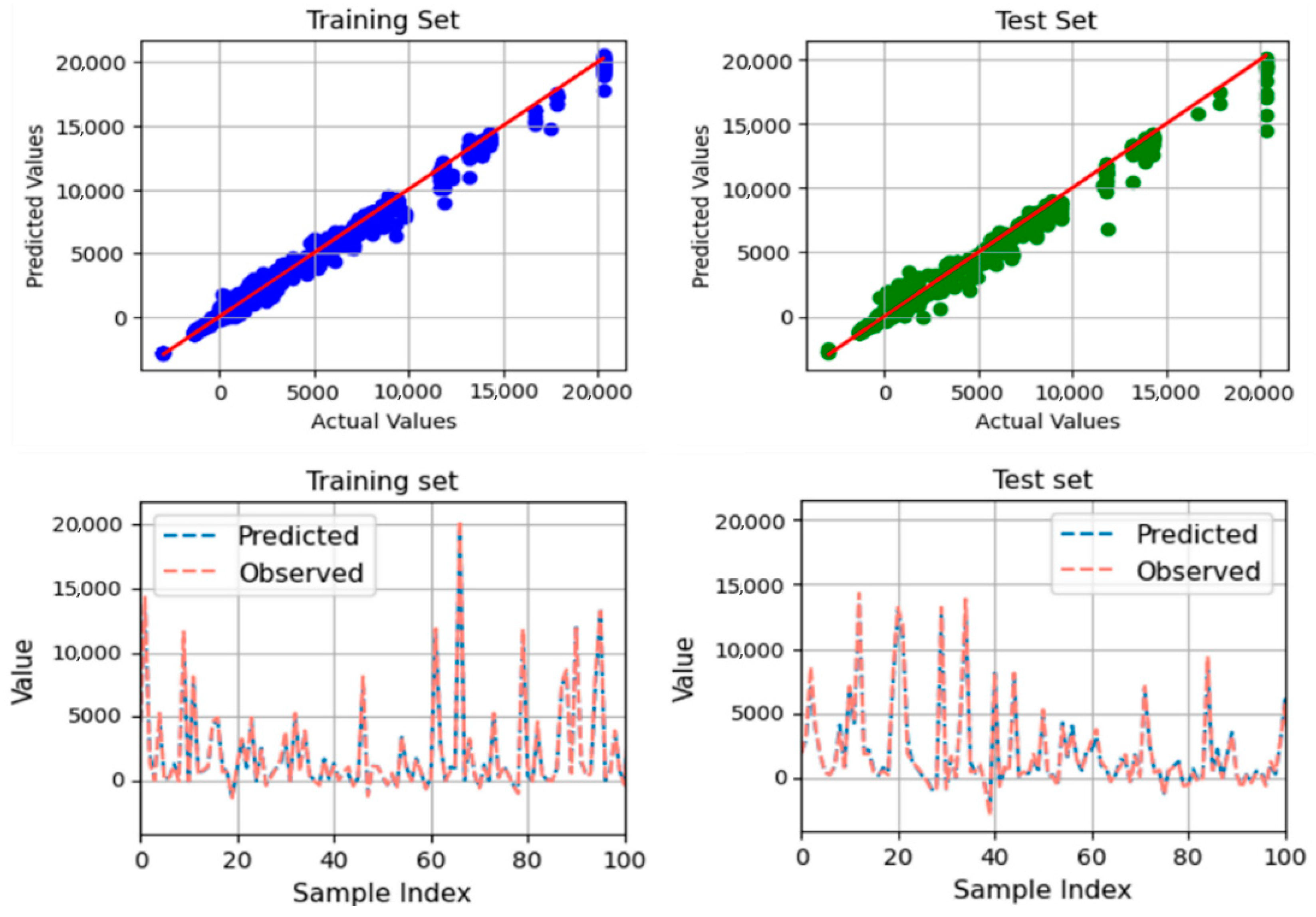
• Another limitation arises from the reliance on historical data, which may not fully capture the rapid advancements in construction technologies and methods. The prediction model is sequentially sampled based on project implementation time, using a training set from 2007 to 2010 and a test set from 2010 to 2011. Consequently, the model can effectively forecast future outputs. Additionally, Figure 5, Figure 6, Figure 7 and Figure 8 illustrate that the model demonstrates accurate predictions within a reasonable range, avoiding extremes that deviate significantly from the mean value. However, the construction industry is evolving, with new materials, techniques, and regulations emerging. These advancements could significantly alter the factors impacting cost adjustments, necessitating continuous updates to the model to maintain its accuracy and relevance.
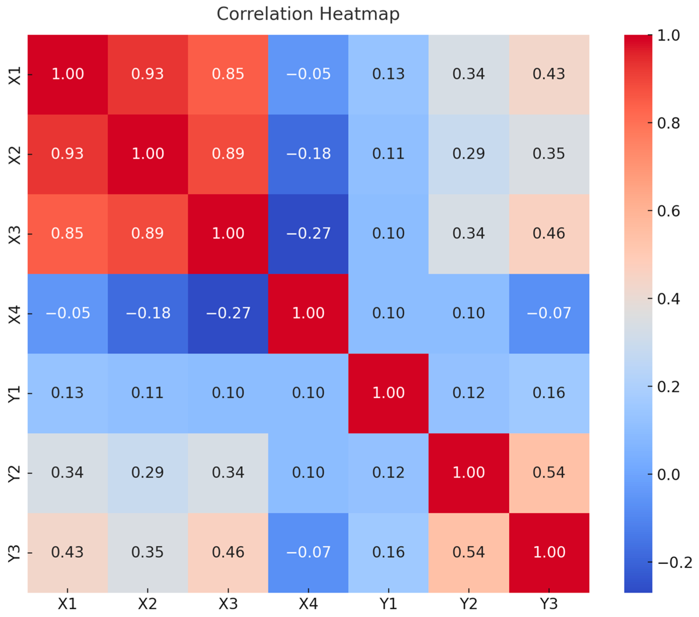
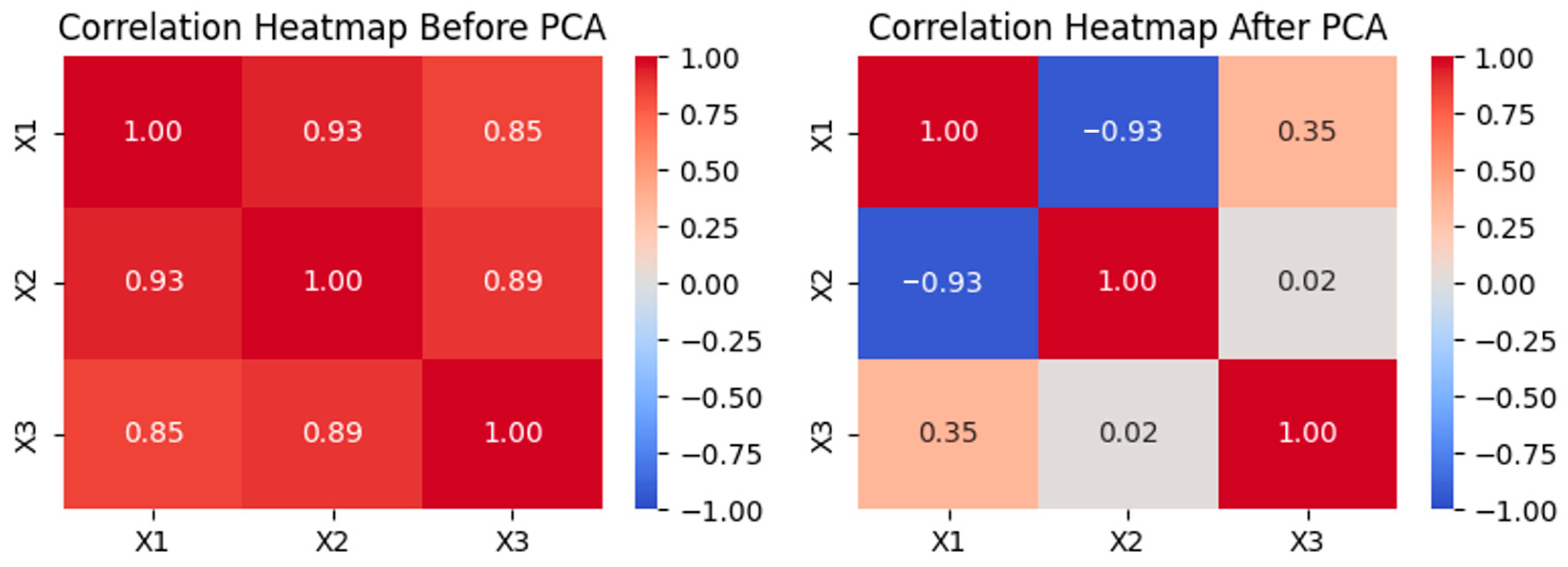
• Finally, the potential for multicollinearity among the variables, despite the application of PCA, suggests that some underlying relationships between predictors may not have been entirely addressed. Future studies could explore alternative or additional dimensionality reduction techniques to further mitigate this issue.

7. Conclusions

This study aimed to create a model that predicts cost changes in apartment construction projects because of design changes. It combined ML and NLP methods. By looking at a large dataset of 35,194 design change instances, narrowed down to 6323 relevant ones through careful cleaning, this research sheds light on how to manage construction project costs when designs change.

The findings showed that ML and NLP are very useful for predicting how design changes affect project costs. The XGBoost model demonstrates a strong predictive performance, with an R-square value of 0.930, indicating that it explains 93% of the variance in cost changes due to design variations. For the overall project cost predictions, including market price fluctuations, the models show excellent reliability, explaining 98.5% of the variance, with an R-square value of 0.985. When excluding price fluctuations, they continue to perform robustly, with an R-square value of 0.982. These models significantly exceed the typical maximum allowable error rate of 20% in the standard cost estimates [32]. The integration of NLP techniques, such as text decomposition, Parts-of-Speech tagging, and TFIDF vectorization, enhances the handling of unstructured data, improving the accuracy of the models.

The “Cost Change by Factor” model is highly accurate (93%) in general cases. However, it struggles with design changes that have a large range of cost increases or decreases (41%). This result highlights the need for new algorithms and evaluation methods specifically tailored to handle the noisy data associated with significant design changes. These improvements will ensure more reliable predictions across a broader spectrum of scenarios.

This study also showed how important it is to clean the data properly before using it in models. This included using the Yeo-Johnson transformation and PCA to fix issues with skewed data and variables that are too closely related. These steps made sure the models worked well with the data, capturing the complex ways design changes can impact costs.

Additionally, the research found that a combined model using CatBoost and SVM worked well for predicting cost changes, considering price changes or not. This approach used the strengths of both algorithms to deal with closely related variables and showed the ability to predict across different datasets.

References

1. Kim, G.H.; Shin, J.; Kim, S.Y.; Shin, Y. Comparison of School Building Construction Costs Estimation Methods Using Regression Analysis, Neural Network, and Support Vector Machine. J. Build. Constr. Plan. Res. 2013, 1, 29576. [Google Scholar] [CrossRef]
2. Amoruso, F.M.; Dietrich, U.; Schuetze, T. Indoor thermal comfort improvement through the integrated BIM-parametric workflow-based sustainable renovation of an exemplary apartment in Seoul, Korea. Sustainability 2019, 11, 3950. [Google Scholar] [CrossRef]
3. Kim, M.; Lee, J.; Kim, J. Analysis of Design Change Mechanism in Apartment Housing Projects Using Association Rule Mining (ARM) Model. Appl. Sci. 2022, 12, 11036. [Google Scholar] [CrossRef]
4. Gharaibeh, L.; Matarneh, S.T.; Arafeh, M.; Sweis, G. Factors Leading to Design Changes in Jordanian Construction Projects. Int. J. Product. Perform. Manag. 2020, 70, 893–915. [Google Scholar] [CrossRef]
5. Yap, J.B.H.; Abdul-Rahman, H.; Chen, W. A Conceptual Framework for Managing Design Changes in Building Construction. MATEC Web Conf. 2016, 66, 00021. [Google Scholar] [CrossRef]
6. Khanh, H.D. Factors Causing Design Changes in Vietnamese Residential Construction Projects: An Evaluation and Comparison. J. Sci. Technol. Civ. Eng. (Stce)-Huce 2020, 14, 151–166. [Google Scholar] [CrossRef]
7. Aslam, M.; Baffoe-Twum, E.; Saleem, F. Design Changes in Construction Projects—Causes and Impact on the Cost. Civ. Eng. J. 2019, 5, 1647–1655. [Google Scholar] [CrossRef]
8. Jafari, P.; Al Hattab, M.; Mohamed, E.; AbouRizk, S. Automated extraction and time-cost prediction of contractual reporting requirements in construction using natural language processing and simulation. Appl. Sci. 2021, 11, 6188. [Google Scholar] [CrossRef]
9. Sánchez, O.; Castañeda, K.; Herrera, R.; Pellicer, E. Benefits of Building Information Modeling in Road Projects for Cost Overrun Factors Mitigation. In Proceedings of the Construction Research Congress 2022, Arlington, VA, USA, 9–12 March 2022. [Google Scholar] [CrossRef]
10. Plebankiewicz, E. Model of Predicting Cost Overrun in Construction Projects. Sustainability 2018, 10, 4387. [Google Scholar] [CrossRef]
11. Williams, T.R.; Gong, J. Predicting Construction Cost Overruns Using Text Mining, Numerical Data and Ensemble Classifiers. Autom. Constr. 2014, 43, 23–29. [Google Scholar] [CrossRef]
12. Babalola, N.A.J.; Aderogba, A.M.; Adetunji, O.O. Inflation and Cost Overrun in Public Sector Construction Projects in Nigeria. ECS Trans. 2022, 107, 16137. [Google Scholar] [CrossRef]
13. Lee, J.; Yi, J.S. Predicting Project’s Uncertainty Risk in the Bidding Process by Integrating Unstructured Text Data and Structured Numerical Data Using Text Mining. Appl. Sci. 2017, 7, 1141. [Google Scholar] [CrossRef]
14. Saravi, M.E.; Newnes, L.; Mileham, A.R.; Goh, Y.M. Estimating Cost at the Conceptual Design Stage to Optimize Design in Terms of Performance and Cost. In Collaborative Product and Service Life Cycle Management for a Sustainable World: Proceedings of the 15th ISPE International Conference on Concurrent Engineering (CE2008); Springer: London, UK, 2008. [Google Scholar] [CrossRef]
15. Kikwasi, G.J. Claims in Construction Projects: How Causes Are Linked to Effects? J. Eng. Des. Technol. 2021, 21, 1710–1724. [Google Scholar] [CrossRef]
16. Afelete, E.; Jung, W. Causes of Design Change Depending on Power Project-Types in Ghana. Energies 2021, 14, 6871. [Google Scholar] [CrossRef]
17. Elmousalami, H.H. Artificial intelligence and parametric construction cost estimate modeling: State-of-the-art review. J. Constr. Eng. Manag. 2020, 146, 03119008. [Google Scholar] [CrossRef]
18. Juszczyk, M.; Leśniak, A.; Zima, K. ANN Based Approach for Estimation of Construction Costs of Sports Fields. Complexity 2018, 2018, 7952434. [Google Scholar] [CrossRef]
19. Koo, C.; Hong, T.; Hyun, C.-T. The Development of a Construction Cost Prediction Model With Improved Prediction Capacity Using the Advanced CBR Approach. Expert Syst. Appl. 2011, 38, 8597–8606. [Google Scholar] [CrossRef]
20. Alqahtani, A.; Whyte, A. Artificial Neural Networks Incorporating Cost Significant Items Towards Enhancing Estimation for (Life-Cycle) Costing of Construction Projects. Constr. Econ. Build. 2013, 14, 1233–1243. [Google Scholar] [CrossRef]
21. Fernando, N. An Artificial Neural Network (ANN) Approach for Early Cost Estimation of Concrete Bridge Systems in Developing Countries: The Case of Sri Lanka. J. Financ. Manag. Prop. Constr. 2023, 29, 23–51. [Google Scholar] [CrossRef]
22. Alshamrani, O.S. Construction Cost Prediction Model for Conventional and Sustainable College Buildings in North America. J. Taibah Univ. Sci. 2017, 11, 315–323. [Google Scholar] [CrossRef]
23. Magdum, S.K.; Adamuthe, A.C. Construction Cost Prediction Using Neural Networks. Ictact J. Soft Comput. 2017, 8, 1. [Google Scholar] [CrossRef]
24. Petruseva, S.; Žileska-Pančovska, V.; Žujo, V.; Brkan-Vejzović, A. Construction Costs Forecasting: Comparison of the Accuracy of Linear Regression and Support Vector Machine Models. Teh. Vjesn.-Tech. Gaz. 2017, 24, 14311438. [Google Scholar] [CrossRef]
25. Surenth, S.; Rajapakshe, R.M.P.P.V.; Muthumala, I.S.; Samarawickrama, M.N.C. Cost Forecasting Analysis on Bored and Cast-in-Situ Piles in Sri Lanka: Case Study at Selected Pile Construction Sites in Colombo Metropolis Area. Eng. J. Inst. Eng. Sri Lanka 2019, LII, 57–66. [Google Scholar] [CrossRef]
26. Ahmed, S.F.; Ali, N.S. Pre-Design Cost Modeling of Road Projects. Tikrit J. Eng. Sci. 2020, 27, 6–11. [Google Scholar] [CrossRef]
27. Ashuri, B.; Lu, J. Time series analysis of ENR construction cost index. J. Constr. Eng. Manag. 2010, 136, 1227–1237. [Google Scholar] [CrossRef]
28. Aydınlı, S. Time Series Analysis of Building Construction Cost Index in Türkiye. J. Constr. Eng. Manag. Innov. 2022, 5, 218–227. [Google Scholar] [CrossRef]
29. Isikdag, U.; Hepsağ, A.; Bıyıklı, S.İ.; Öz, D.; Bekdaş, G.; Geem, Z.W. Estimating Construction Material Indices With ARIMA and Optimized NARNETs. Comput. Mater. Contin. 2023, 74, 113. [Google Scholar] [CrossRef]
30. Wang, J.; Ashuri, B. Predicting ENR construction cost index using machine-learning algorithms. Int. J. Constr. Educ. Res. 2017, 13, 47–63. [Google Scholar] [CrossRef]
31. Fan, M.; Sharma, A. Design and Implementation of Construction Cost Prediction Model Based on SVM and LSSVM in Industries 4.0. Int. J. Intell. Comput. Cybern. 2021, 14, 145–157. [Google Scholar] [CrossRef]
32. Meharie, M.G.; Mengesha, W.J.; Gariy, Z.A.; Mutuku, R.N. Application of Stacking Ensemble Machine Learning Algorithm in Predicting the Cost of Highway Construction Projects. Eng. Constr. Archit. Manag. 2021, 29, 2836–2853. [Google Scholar] [CrossRef]
33. Hsu, M.-W.; Dacre, N.; Senyo, P.K. Identifying Inter-Project Relationships With Recurrent Neural Networks: Towards an AI Framework of Project Success Prediction. SSRN Electron. J. 2021. [Google Scholar] [CrossRef]
34. Ahn, S.H.; Altaf, M.S.; Han, S.; Al-Hussein, M. Application of Machine Learning Approach for Logistics Cost Estimation in Panelized Construction. Modul. Offsite Constr. (Moc) Summit Proc. 2017. [Google Scholar] [CrossRef]
35. Cheng, M.-Y.; Hoang, N.-D. Interval Estimation of Construction Cost at Completion Using Least Squares Support Vector Machine. J. Civ. Eng. Manag. 2014, 20, 223–236. [Google Scholar] [CrossRef]
36. Hashemi, S.T.; Ebadati, O.M.; Kaur, H. Cost Estimation and Prediction in Construction Projects: A Systematic Review on Machine Learning Techniques. SN Appl. Sci. 2020, 2, 1703. [Google Scholar] [CrossRef]
37. Sharma, S.; Ahmed, S.; Naseem, M.; Alnumay, W.S.; Singh, S.; Cho, G. A Survey on Applications of Artificial Intelligence for Pre-Parametric Project Cost and Soil Shear-Strength Estimation in Construction and Geotechnical Engineering. Sensors 2021, 21, 463. [Google Scholar] [CrossRef] [PubMed]
38. Al Shalabi, L.; Shaaban, Z.; Kasasbeh, B. Data mining: A preprocessing engine. J. Comput. Sci. 2006, 2, 735–739. [Google Scholar] [CrossRef]
39. Benavoli, A.; Corani, G.; Mangili, F. Should we really use post-hoc tests based on mean-ranks? J. Mach. Learn. Res. 2016, 17, 152–161. [Google Scholar]
40. Walkowiak, T.; Gniewkowski, M. Evaluation of vector embedding models in clustering of text documents. In Proceedings of the International Conference on Recent Advances in Natural Language Processing (RANLP 2019), Varna, Bulgaria, 2–4 September 2019; pp. 1304–1311. [Google Scholar]
41. Bisandu, D.B.; Moulitsas, I.; Filippone, S. Social ski driver conditional autoregressive-based deep learning classifier for flight delay prediction. Neural Comput. Appl. 2022, 34, 8777–8802. [Google Scholar] [CrossRef]
42. Kyriazos, T.; Poga, M. Dealing with multicollinearity in factor analysis: The problem, detections, and solutions. Open J. Stat. 2023, 13, 404–424. [Google Scholar] [CrossRef]
43. Gwelo, A.S. Principal components to overcome multicollinearity problem. Oradea J. Bus. Econ. 2019, 4, 79–91. [Google Scholar] [CrossRef]
44. Deshpande, N.; Londhe, S.; Kulkarni, S. Modeling compressive strength of recycled aggregate concrete by Artificial Neural Network, Model Tree and Non-linear Regression. Int. J. Sustain. Built Environ. 2014, 3, 187–198. [Google Scholar] [CrossRef]
45. Lin, P.; Ding, F.; Hu, G.; Li, C.; Xiao, Y.; Tse, K.T.; Kwok, K.; Kareem, A. Machine learning-enabled estimation of crosswind load effect on tall buildings. J. Wind Eng. Ind. Aerodyn. 2022, 220, 104860. [Google Scholar] [CrossRef]
46. Chen, T.; Guestrin, C. Xgboost: A scalable tree boosting system. In Proceedings of the 22nd Acm Sigkdd International Conference on Knowledge Discovery and Data Mining, San Francisco, CA, USA, 13–17 August 2016; pp. 785–794. [Google Scholar]
47. Shah, S.F.A.; Chen, B.; Zahid, M.; Ahmad, M.R. Compressive strength prediction of one-part alkali activated material enabled by interpretable machine learning. Constr. Build. Mater. 2022, 360, 129534. [Google Scholar] [CrossRef]
48. Dorogush, A.V.; Ershov, V.; Gulin, A. CatBoost: Gradient boosting with categorical features support. arXiv 2018, arXiv:1810.11363. [Google Scholar]
Figure 1. The process of developing a model to predict cost changes due to design changes.
Sustainability 16 04322 g001
Figure 2. Correlation heatmap of the numeric variables.
Sustainability 16 04322 g002
Figure 3. Distribution of the numeric data before and after Yeo-Johnson transformation.
Sustainability 16 04322 g003
Figure 4. Correlation of X1, X2, and X3 before and after PCA.
Sustainability 16 04322 g004
Figure 5. Model performance of the XGB model (OP1).
Sustainability 16 04322 g005
Figure 6. Performance of the MLR model (OP1).
Sustainability 16 04322 g006
Figure 7. Performance of the stacked model in OP2.
Sustainability 16 04322 g007
Figure 8. Performance of the stacked model in OP3.
Sustainability 16 04322 g008