Shanghai Transport Carbon Emission Forecasting Study Based on CEEMD-IWOA-KELM Model

Abstract

In the light of the worsening of, and the adverse effects produced by, global warming, a study of Shanghai’s transport carbon emissions can provide an advanced model that can be replicated throughout other cities, thus assisting in the management and reduction of carbon emissions. Considering the volatility and nonlinearity of the carbon emission data series of the transport industry, a prediction model combining complementary ensemble empirical modal decomposition (CEEMD), the improved whale optimization algorithm (IWOA), and the Kernel Extreme Learning Machine (KELM) is proposed for a more accurate prediction of the forecasting of carbon emissions from Shanghai’s transport sector. First, nine indicators were screened as the influencing factors of Shanghai’s transport carbon emissions through the STIRPAT model, and the corresponding carbon emissions were calculated with data related to Shanghai’s transport carbon emissions from 1995 to 2019; Secondly, CEEMD was used to decompose the original data into multiple smooth series and one residual term, and KELM was applied to build a prediction model for each decomposition result, and IWOA was used to optimize the model parameters. The experimental results also demonstrate that CEEMD can effectively reduce model errors. Comparative experiments show that the IWOA algorithm can significantly enhance the stability of machine learning models. The outcomes of various experiments indicate that the CEEMD-IWOA-KELM model produces optimal results with the highest accuracy. Additionally, this model exhibits high stability, as it provides a wider range of methods for predicting carbon emissions and contributing to carbon reduction targets.

1. Introduction

As Joseph Fourier first proposed the concept of the greenhouse effect in 1824, scientific research into global warming has spanned nearly 200 years [1]. Global warming has led to an increase in extreme weather events, posing a threat to human survival and societal development. Consequently, China has put forward the “dual carbon” goals of reaching peak carbon emissions by 2030 and achieving carbon neutrality by 2060. The transportation sector is the third-largest source of carbon emissions in China, with emissions continuing to rise annually [2]. As one of the largest and most developed cities in China, Shanghai, with its dense population and high level of economic activity, should proactively respond to the “dual carbon” initiative, making energy conservation and emission reduction a key policy [3]. Moreover, Shanghai has committed to peaking its carbon emissions by 2025, five years ahead of the national target. Research into Shanghai’s carbon emissions is significant for understanding global climate change. Particularly in the transportation sector, the issue of vehicle emissions highlights the necessity of exploring predictive models and reduction strategies for transportation-related carbon emissions, which hold valuable lessons for other regions. Therefore, it is essential to develop a highly accurate predictive model for transportation carbon emissions to forecast future trends in Shanghai’s transportation sector and formulate appropriate reduction strategies based on these trends and data, promoting a shift towards a greener, more sustainable, and low-carbon transportation system in China [4].

This paper proposes a transport carbon emission prediction model combining complementary ensemble empirical modal decomposition, the improved whale optimization algorithm, and the kernel limit learning machine model. Firstly, nine indicators are screened by the STIRPAT (Stochastic Impacts by Regression on Population, Affluence, and Technology) model as the influencing factors of Shanghai’s transport carbon emissions. Secondly, the original carbon emission data were decomposed into several internal modal components with different amplitudes and a residual term by CEEMD, and the smooth signal obtained from the decomposition was used as input to optimize the weights and bias values of the hidden nodes of the KELM model by IWOA, to predict the transport carbon emissions of Shanghai. The weights and bias values of the hidden nodes of the KELM model were optimized by IWOA to improve the prediction accuracy of the model; finally, the CEEMD-IWOA-KELM model is compared and analyzed with other models, and the result proves that the method proposed in this paper has a higher prediction accuracy.

This study, through various experiments, concludes that CEEMD can effectively reduce errors. Furthermore, the innovative CEEMD-IWOA-KELM model proposed in this study further reduces errors compared to earlier research. Additionally, this model can extend the methods for predicting carbon emissions.

2. Related Works

Research on the measurement of carbon emissions from transportation is problematic due to the lack of official data and the difficulty in obtaining data for ‘bottom-up’ data. Moreover, data with a lower accuracy can lead to a lower accuracy in calculating transportation carbon emissions. Therefore, this study uses a “top-down” method for calculating the total transportation carbon emissions. In terms of carbon emission influencing factors, the STIRPAT model is a verified model that has many areas of application and influencing factors that are rigorously determined. Wang Qingrong [4] and others also used the STIRPAT model to select eight types of variables as the influencing factors of carbon emissions from China’s transport industry in their research.

Regarding research in the field of carbon emission prediction, the research hotspots can be summarized as unidimensional prediction and multidimensional prediction. A unidimensional prediction is mainly based on time series data and the characteristics of the carbon emission data themselves, so the main aim of the research is the innovation of prediction methods in order to obtain prediction results with a lower error. Yang et al. [5] studied the carbon emissions of passenger flights in Shanghai by using the Autoregressive Integrated Moving Average (ARIMA) model to predict the consumption of air transportation fuel and carbon emissions from 2017 to 2022. Xinyi Huang et al. [6] established a Gray Model (GM) prediction model to predict carbon emissions in Jiangsu Province for five years, but the simple GM (1, 1) model could not accurately reflect the relationship between the dependent and independent variables. The unidimensional forecasting study has several limitations. It is unable to predict technological innovations based on carbon emissions data in a single data column, and it is unable to account for the potential impact of external variables. As a result, the prediction conclusion may not be as comprehensive as they could be and may not accurately reflect the relationship between carbon emissions factors and carbon emissions.

In contrast, the multidimensional prediction of carbon emissions has become a research hotspot for scholars at home in China and abroad due to the consideration of the influence of external factors such as population and energy on carbon emissions, especially with the use of neural network algorithms, which have received more and more attention in the field of carbon emissions prediction. For example, Yang Wenli and Yan Zhengang [7] established a CO₂ emission prediction model for farmland soil based on the Radial Basis Function (RBF) network algorithm; however, the RBF neural network algorithm is difficult in terms of parameter selection, and the computational complexity is high. Turson-Buyouti et al. [8] applied a Generalized Regression Neural Network (GRNN) to construct an emission prediction model, although the GRNN algorithm has a high computational complexity and poor interpretability. Di Zhang [9] and others established Improved Particle Swarm Optimization (IPSO) to optimize the backpropagation (BP) neural network model to simulate and predict the carbon emissions and emission intensity of Shandong Province, but the BP neural network is slow to learn and prone to fall into local minima. Lian Yanqiong et al. [10] used a CNN-LSTM neural network hybrid model to predict the carbon emissions of Fujian Province from 2022 to 2035. Huang et al. [11] proposed the Kernel Extreme Learning Machine (KELM) model, which introduces the kernel function into the basic Extreme Learning Machine (ELM) model. According to the existing research, the KELM model is more flexible in adapting to different types of data and problems and has a wider scope of application than the ELM model. Zhang Xinsheng [12] and others used the KELM model to improve the accuracy of carbon emission prediction. The models and their characteristics are summarized in Table 1.

Table 1. Model name and its features.

Model Name	Reference	Algorithm Features
ARIMA	Yang et al. [5]	While the model demonstrates a good fit for time series data, it lacks the capability to integrate other influencing factors.
GM (1, 1)	Huang et al. [6]	The model lacks the ability to accurately capture the relationship between the dependent and independent variables.
RBF	Yang Wenli and Yan Zhengang [7]	The algorithm presents challenges in parameter selection and exhibits high computational complexity.
GRNN	Turson-Buyouti et al. [8]	The algorithm has a high computational complexity and poor interpretability.
BP	Di Zhang [9]	Slow to learn and prone to fall into local minima
LSTM	Lian Yanqiong et al. [10]	Very suitable for handling time series prediction, but with a long training time and difficult debugging
KELM	Zhang Xinsheng [12]	More flexible in adapting to different types of data and problems

To address the issue of prediction models easily getting trapped in local optima and to tackle increasingly complex optimization problems, hundreds of intelligent optimization algorithms have emerged internationally. According to the research by Xu Ting [13], among these, swarm intelligence optimization algorithms have a broader range of applications. Due to their characteristics, such as their simplicity of mechanism, fewer variables, ease of implementation, and good generalization capabilities, swarm intelligence optimization algorithms have gained popularity among researchers across various fields. Many studies [12,14,15,16] also mention that swarm intelligence optimization algorithms are better suited for carbon emission prediction. Mao Hanshen [17] used Cuckoo Search (CS) to solve the problem of the local optimality of the BP neural network due to the random values of parameters and improved the predictive ability of the model. Jiajun Jiao and Tianyuan Liu [18] used the Improved Adaptive White Noise Complete Intrinsic Computing Expressive Empirical Mode Decomposition with Adaptive Noise (ICEEMDAN) and Improved Whale Optimization Algorithm (IWOA), and Bidirectional Long Short-Term Memory (BiLSTM) prediction models obtained better prediction results than other single benchmark models and most of the combined models. The improved whale optimization algorithm initializes the population through a quasi-backward learning approach, which facilitates balancing global search and local exploitation capabilities [19].

Although the prediction model of machine learning combined with the swarm intelligence optimization algorithm has a better accuracy and stability, due to the volatility and nonlinearity of the carbon emission data series itself [20], this problem cannot be eliminated fundamentally, notwithstanding the numerous studies undertaken attempting to optimize the setting of the influencing factors or the use of different prediction methods. To solve the above problems, Zhang Xinsheng [21] and others used complementary ensemble empirical mode decomposition to decompose the original data (CEEMD), applied ELM to establish a prediction model, and used the Sparrow Search Algorithm (SSA) to optimize the model parameters, in which the Extreme Learning Machine model has achieved relatively good results, but the prediction accuracy needs to be improved.

3. Materials and Methods

3.1. Transport Carbon Emission Measurement

3.1.1. Methodology for Measuring Carbon Emissions from Transport

Transport carbon emissions are measured using a ‘top-down’ approach from the IPCC 2006 Guidelines for National Greenhouse Gas Inventories 2019 Revision [22], with Equations (1) and (2).

$$C={\sum }_i{C}_i={\sum }_i{E}_i\times {\mathrm{F}}_i$$

(1)

$${\sum }_i{\mathrm{F}}_i=\mathrm{C}{\mathrm{V}}_i\times \mathrm{A}\mathrm{L}{\mathrm{V}}_i\times \mathrm{C}{\mathrm{F}}_i\times \mathrm{C}\mathrm{O}{\mathrm{F}}_i\times {\displaystyle \frac{44}{12}}$$

(2)

where $i$ represents the type of energy; $C$ represents the total amount of carbon dioxide emissions from the transport sector; $C_i$ denotes the amount of carbon dioxide produced by the ith type of energy consumption; $E_i$ represents the consumption of the $i$ type of energy; ${\mathrm{F}}_i$ denotes the carbon emission factor of the $i$ energy source; $\mathrm{C}{\mathrm{V}}_i$ denotes carbon content per unit of calorific value; $\mathrm{A}\mathrm{L}{\mathrm{V}}_i$ denotes average low-level heat generation; $\mathrm{C}{\mathrm{F}}_i$ denotes the discounted standard coal factor; $\mathrm{C}\mathrm{O}{\mathrm{F}}_i$ denotes the carbon oxidation rate; and 44/12 is the molecular weight of carbon and carbon dioxide. The calculation of energy consumption for electricity is more specific, and the standard coal factor for electricity is 0.1229 kgce/(kwh).

3.1.2. Selection of Factors Affecting Transport Carbon Emissions

To overcome the problem of inconsistency between the independent variables and the dependent variables in the IPAT (Impact, Population, Affluence, and Technology) model, York et al. [23] proposed the STIRPAT model, which has a long history of development and a wide range of applications, and is known for its rigorous factor-screening process; so, this paper uses the STIRPAT model to select the key factors affecting carbon emissions from transport. To further enhance the explanatory power and analytical depth of the model, expansion of the influencing factors has been considered to achieve the enhancement of the model’s effectiveness.

In contrast to Equations (1) and (2) used for carbon emission calculations, the STIRPAT model offers a valuable framework for quantifying and analyzing the impact of various factors on the environment. This is of significant importance for policy-making and environmental protection research. The carbon emissions of the transportation industry are influenced by three dimensions, population, wealth, and technological level. Continuing to expand the STIRPAT model, 9 types of variables were ultimately selected as the main influencing factors. They are population size (P), GDP per capita (A), civilian motor vehicle ownership (VEH), passenger turnover (PT), cargo turnover (GT), urbanization level (U), energy structure (ES), energy intensity (IS), and carbon emission intensity (T). The identified influencing factors are shown in Table 2, and the extended STIRPAT model expression is

I = αP^β1A^β2PT^β3GT^β4VEH^β5T^β6IS^β7ES^β8U^β9ε

(3)

Table 2. Sorting out the factors influencing transport carbon emissions.

Impact Factors	Impact Indicators	Meaning in This Study	References
Demographic Factors	Population Size (P)	Total household population in Shanghai at the end of the year	[4,24,25,26,27,28,29,30,31,32]
	Urbanization Level (U)	Ratio of urban population to total population	[4,26,33,34]
Wealth Factors	GDP per capita (A)	Ratio of Shanghai’s GDP to the total registered population in Shanghai at the end of the year	[4,24,26,27,28,29,30,31,32,33,34]
	Motor Vehicle Ownership (VEH)	Vehicle ownership for civilian use in Shanghai	[4,27,32,33]
	Passenger Turnover (PT)	Passenger traffic volume in Shanghai	[4,25,31,32,34]
	Cargo Turnover (GT)	Cargo turnover in Shanghai	[4,24,31,33,34]
Technology Level	Energy Structure (ES)	Ratio of raw clean energy consumption to all energy consumption in Shanghai region	[28,29,30,31]
	Energy Intensity (IS)	Ratio of Shanghai’s raw energy consumption to Shanghai’s GDP	[4,25,26,27,31,34]
	Carbon Emission Intensity (T)	Ratio of total carbon emissions from the transport sector in the Shanghai region to Shanghai’s GDP	[4,26,27,28,30,32]

In practical analyses, we usually take the logarithm of the left and right parts of Equation (4) and use the reduced power method to calculate them:

lnI = lnα + β₁lnP + β₂lnA + β₃lnPT + β₃lnGT + β₅lnVEH + β₆lnT + β₇lnIS + β₈lnES + β₉lnU + lnε

(4)

where I denotes carbon emissions from transport; α is a constant; P denotes total population; A denotes GDP per capita; PT denotes passenger turnover; GT denotes freight turnover; VEH denotes civilian car ownership; T denotes carbon emission intensity; IS denotes energy intensity; ES denotes the energy use structure; U stands for the degree of urbanization; and ε is a stochastic perturbation factor. According to the theory of elasticity coefficients, the coefficients in the regression equation actually reveal the elastic link between the dependent and independent variables; β₁, β₂, β₃, β₄, β₅, β₆, β₇, β₈, β₉ are the elasticity coefficients, and keeping the other independent variables unchanged, a 1% change in P, A, PT, GT, VEH, T, IS, ES, U, respectively, causes β₁%, β₂%, β₃%, β₄%, β₅%, β₆%, β₇%, β₈%, and β₉% changes.

In this paper, the Pearson product–moment correlation coefficient is used simultaneously with the selection of influencing factors to test their linear correlation with carbon emissions. Pearson correlation analysis is a statistical method used to assess the strength and direction of the linear relationship between two continuous variables, and the closer the absolute value of the correlation coefficient is to 1, the stronger the correlation between the feature and carbon emissions. As shown in Figure 1, the absolute values of D Pearson correlation coefficients between the above selected factors and transport carbon emissions are all greater than 0.80, which is close to 1. It can be concluded that there is a strong linear correlation between the selected influencing factors in this paper and transport carbon emissions. In the Pearson correlation analysis, ***, **, and * represent significance levels of 1%, 5%, and 10%, respectively. In Figure 1, *** represents p < 0.001, indicating that the marked significance level is statistically significant.

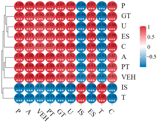
Figure 1. Heat map of Pearson’s correlation coefficients.

3.1.3. Data Sources

Based on the literature [23,24,25,26,27,28,29,30,31,33,34], this study selects seven types of energy for the calculation of total transportation carbon emissions. The selected energy sources are raw coal, crude oil, gasoline, kerosene, diesel, fuel oil, and electricity consumption. The data utilized for this analysis were obtained from the official website of the National Bureau of Statistics of China, pertaining specifically to the Shanghai region.

The indicator calculation aspects of this paper use population number, GDP per capita, and urbanization rate data taken from the Shanghai Statistical Yearbook (but because Shanghai since 2016, to abolish the nature of the distinction between agricultural and non-agricultural households in Shanghai, unified for the residents of the household, the urbanization rate according to the national urbanization process and the prediction of the urbanization process of Shanghai in the past years is difficult to obtain); passenger turnover, cargo turnover, motor vehicle ownership, carbon emission intensity, energy intensity, and energy use structure were obtained from the China Energy Statistics Yearbook and the website of the National Bureau of Statistics. The carbon content, low-level heat content, standard coal factor, and carbon oxidation rate of various energy sources were obtained from the “Statistical Survey System of Energy Resource Consumption in Public Institutions”; the correlation coefficients of the various energy sources are shown in Table 2, and the total carbon emissions of Shanghai’s transport in the period of 1995–2019 can be obtained by using data in Equations (1) and (2) and Table 3. The carbon content refers to the amount of carbon emissions per unit of heat generated during the combustion process. The lower heating value (LHV) refers to the amount of heat produced by the complete combustion of a unit mass of fuel. The standard coal conversion factor indicates how many kilograms of standard coal a unit mass of energy can be converted into. The carbon oxidation rate refers to the proportion of carbon in the fuel that is oxidized into carbon dioxide during the combustion process, as shown in Table 4. The calculation of electricity consumption is quite unique, as it only requires multiplying the carbon emission factor by the amount of electricity consumed. The conversion coefficient of electricity to standard coal is 0.1229 kgce/(kWh).

Table 3. Correlation coefficients for various energy sources.

Energy	Carbon Content (kg/GJ)	Lower Heating Value (kJ/kg)	Standard Coal Conversion Factor (kgce/kg)	Carbon Oxidation Rate (%)
Crude coal	29.2	20,934	0.7143	98
Crude oil	20.0	41,868	1.4286	99
Petrol	18.9	43,124	1.4714	99
Paraffin	19.6	43,124	1.4714	99
Diesel oil	20.2	42,705	1.4571	99
Fuel oil	21.1	41,868	1.4286	99

Table 4. Carbon emissions from transport.

Year	Carbon Emissions/10 kt	Year	Carbon Emissions/10 kt
1995	2277.48	2008	2599.63
1996	2438.67	2009	2608.21
1997	2418.16	2010	2829.28
1998	2457.87	2011	2880.87
1999	2599.63	2012	2865.03
2000	2608.21	2013	3037.40
2001	2829.28	2014	2749.53
2002	2880.87	2015	2887.64
2003	2865.03	2016	2915.67
2004	2277.48	2017	2994.37
2005	2438.67	2018	2779.69
2006	2418.16	2019	2905.12
2007	2457.87

3.2. Data Preprocessing

Empirical mode decomposition (EMD), first introduced in 1998 by Huang et al. [35], is a technique that can convert complex nonlinear time series data into a series of simple, convergent, and stable components, i.e., the intrinsic mode function (IMF) and a residual component (Res). Subsequently, Wu et al. [36] obtained the final decomposition result by superimposing white noise onto the original series several times and averaging the IMF, called ensemble empirical mode decomposition (EEMD), as an improved scheme to effectively alleviate the mode aliasing problem in EMD, but the output of the method is particularly sensitive to the superimposed noise. To overcome this limitation, Yeh et al. [37] improved the algorithm again and proposed CEEMD, which can reduce the information loss and enhance the stability and accuracy of the decomposition by adding randomly initialized white noise sequences to the original signal several times. The specific steps of CEEMD are as follows:

Add N pairs of normally distributed positive and negative white noise sequences to the original data sequence by Equation (5).

$$\left[{\displaystyle \genfrac{}{}{0pt}{}{M_1}{M_2}}\right]=\left[{\displaystyle \genfrac{}{}{0pt}{}{1}{1}}{\displaystyle \genfrac{}{}{0pt}{}{1}{-1}}\right]\left[{\displaystyle \genfrac{}{}{0pt}{}{S}{N}}\right]$$

(5)

where S represents the original signal to be decomposed, N represents the introduced Gaussian white noise, and M₁ and M₂ represent the new signals synthesized from the original signal S and the positive and negative Gaussian white noise. Next, the constructed target signals are decomposed using EMD, and each signal is decomposed to produce a series of IMF components, whereby ${imf}_j$ denotes the i of the j IMF components. At the end stage, all the IMF components containing noise are summarized, and the average value is calculated to obtain the final stabilization result of each IMF; the specific formula is as Equation (6).

$${imf}_j={\displaystyle \frac{1}{2N}}{\sum }_{i=1}^{2N}{imf}_{ij}$$

(6)

In summary, the final decomposition result x(t) of CEEMD is shown by Equation (7).

$$x\left(t\right)={\sum }_{j=1}^K{imf}_j\left(t\right)+res$$

(7)

3.3. Parameter Optimization

The whale optimization algorithm (WOA) was first proposed by Mirjalili and Lewis in 2016 [38]. While many optimization algorithms use a single position adjustment strategy, WOA features three dynamic search strategies, namely encircling predation, spiral bubble-net predation, and random search predation, to adjust the positions of searching individuals, and its strategy operation mechanism is shown in Figure 2. WOA demonstrates an excellent global search capability by virtue of these diversified strategies, but this leads inevitably to lengthening the convergence time, and it is easier to obtain local optimal solutions during the iterative process. To address these limitations, Wu Zequan and Mou Yongmin [19] proposed an improved whale optimization algorithm (IWOA) by improving the WOA via three core dimensions: optimizing the initial population generation mechanism, improving the position-updating rules, and designing a specialized mechanism for avoiding falling into the local optimum solution.

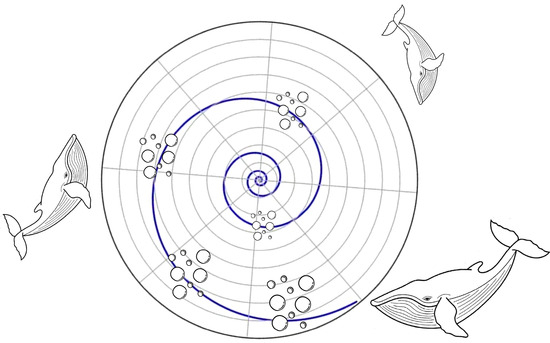
Figure 2. Operational mechanisms of humpback whale bubble-net predation.

3.4. Machine Learning Model Selection

3.4.1. Kernel Extreme Learning Machine

KELM, as an extension of the ELM proposed by Huang et al. [39], is Single Hidden Layer Feedforward Neural network (SLFN)-based. To address the possible limitations of ELM due to random initialization, KELM incorporates the kernel function theory in the base ELM, which enables the optimal least squares solution to be obtained. Thanks to the kernel function, KELM can automatically adapt to and handle nonlinear data, based on the principle of mapping the original input data into a higher-dimensional feature space to achieve the linear transformation of complex nonlinear relationships, which is superior for solving the highly nonlinear problems in the neighborhood of carbon emissions. The network structure of KELM and ELM is shown in Figure 3.

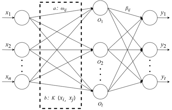
Figure 3. ELM and KELM schematic.

In the figure, a is the mapping function of ELM and b is the mapping function of KELM. Entering from the left side $x_n$ is the amount of input data, assuming that there are n neurons in the input layer, l neurons in the hidden layer, t neurons in the output layer, the connection weights ${\omega }_{ij}$ between the input layer and the hidden layer and the threshold $O_l$ in the hidden layer, and ${\beta }_{ij}$ denotes the output weights. The ELM can be represented by Equation (8).

$$\beta ={\mathit{H}}^{+}T$$

(8)

where ${\mathit{H}}^{+}$ denotes the Moore–Penrose Generalized Inverse Matrix (MGIM) of matrix $\mathit{H}$. The regularization coefficient C in KELM is primarily used to control the degree of regularization. A higher value of C means the model is more inclined to fit the training data, which may lead to overfitting. A lower value of C, on the other hand, suggests that the model prioritizes generalization capability, but this may result in underfitting. The optimal value of C can be determined through methods such as cross-validation or intelligent optimization algorithms. And the optimization stage weights β can be evolved through the regularization factor C by Equation (9).

$$\beta ={\mathit{H}}^T{\left({\mathit{H}\mathit{H}}^T+{\displaystyle \frac{\mathit{I}}{C}}\right)}^{-1}T$$

(9)

where i is the N-dimensional unit matrix. Under the condition that the hidden layer feature mapping h(·) is unknown, the kernel matrix in KELM can be expressed by Equation (10).

$$\mathit{\Omega }={\mathit{H}\mathit{H}}^T:{\mathit{\Omega }}_{\mathbf{r}\mathbf{e}\mathbf{s}\mathbf{u}\mathbf{r}\mathbf{i}\mathbf{s}}=h\left(x_i\right)·h\left(x_j\right)$$

(10)

In summary, the output function of KELM can be expressed by Equation (11).

$$f\left(x\right)=h\left(x\right)·\beta =h\left(x\right)·{\mathit{H}}^T{\left({\mathit{H}\mathit{H}}^T+{\displaystyle \frac{\mathit{I}}{C}}\right)}^{-1}T=\left|\begin{array}{c}K\left(x,x_1\right)\\ \begin{array}{c}·\\ ·\\ ·\end{array}\\ K\left(x,x_N\right)\end{array}\right|{\left({\mathit{\Omega }}_{xlM}+{\displaystyle \frac{\mathit{I}}{C}}\right)}^{-1}T$$

(11)

3.4.2. Other Neutral Network Prediction Models

In existing research, artificial neural network technology has become a common tool for carbon emission prediction, but given that various types of models have their own application scenarios and performance differences, it is especially critical to choose the right model and tailor the carbon emission prediction scheme according to the unique properties of different neural network models. In the carbon emission prediction research focusing on the transport sector, in addition to the ELM model, the BP neural network model and the Long Short-Term Memory (LSTM) model are also widely used, and the GRNN model has also appeared in the existing research.

A BP neural network is a multi-layer feedforward neural network with the backward propagation of errors consisting of input, hidden, and output layers [40]. BP neural network model signals are transmitted in the forward direction with a full interconnection between layers. The error between the output value and the target value is transmitted in the reverse direction, and the weights and thresholds of the BP neural network can be adjusted by means of transmission from the output layer through the implicit layer to the input layer, and the whole learning process will be stopped after continuous iterative learning when the error reaches the set very small value or the set iteration value.

Long Short-Term Memory (LSTM) [41] is an evolution and deepening of Recurrent Neural Network (RNN) architecture, adding core components such as input gates, forgetting gates, output gates, and memory cells, which effectively overcome the challenges of RNNs in dealing with fluctuations. The LSTM model is good at handling time series prediction tasks with large fluctuations and significant trend changes because it can capture and adapt to the sharp fluctuations in the trend in the data series well.

A Generalized Regression Neural Network (GRNN) consists of four layers: an input layer, pattern layer, summation layer, and output layer. The BP algorithm is used to train the network connection weights, relying on data samples for training and learning, and there is only one threshold for human-adjusted parameters, which can greatly avoid the influence of subjective factors on the prediction results [42].

3.5. Construction of Carbon Emission Prediction Models for Transport

Given the special nonlinearity and volatility of transport carbon emission data, such complex data have certain limitations in the application of traditional prediction models. To solve the above problems, this paper constructs a CEEMD-IWOA-KELM composite prediction model based on CEEMD technology, the IWOA optimization algorithm, and the KELM model. The flow of steps for the construction and implementation of this model is shown in Figure 4.

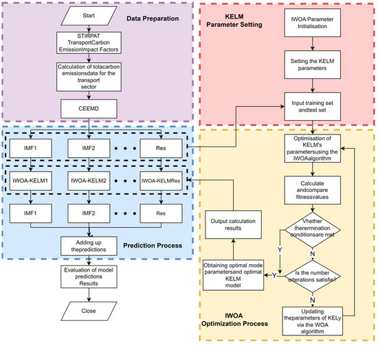
Figure 4. Carbon emission prediction model based on CEEMD-IWOA-KELM for the transport sector.

(1)

Adopt the STIRPAT model for transport carbon emission factors, consider the influencing factors from the population factors, wealth factors, and technology level, and finally select a total of 9 types of variables as the main influencing factors, including P, U, A, VEH, PT, GT, ES, IS, and T.

(2)

Calculate the total carbon emissions C of Shanghai’s transport industry according to Equation (1).

(3)

Decompose the original transport carbon emission data by the CEEMD method, and separate out the internal modal component ${imf}_j$ and the residual part Res.

(4)

Adjust the initial parameters of the IWOA algorithm and the KELM model, and update the position of the whale population in the search space by means of Equations (6)~(11); meanwhile, establish the KELM prediction model by means of Equations (12)~(15).

(5)

For each decomposed ${imf}_j$ and Res, establish an IWOA-KELM prediction model, and obtain the predicted output value of each decomposed sequence through optimal selection of parameters.

(6)

Combine the forecasts of all the decomposed sequences to obtain the forecast value of total carbon emissions from the Shanghai transport industry.

(7)

Compare the obtained prediction values with the actual measured data, quantify the prediction errors by calculating the error indicators, and analyze them in depth to assess the validity and reliability of the model.

In summary, this study employs the STIRPAT model to analyze the influencing factors of carbon emissions in the transportation sector. It utilizes the CEEMD method to decompose the original carbon emission data and employs the optimized IWOA-KELM model to predict the individual modal components. Finally, it integrates the prediction results to evaluate the total carbon emissions of the transportation industry in Shanghai. The accuracy of the predictions is quantified using error metrics to validate the effectiveness and reliability of the model.

4. Results

All experimental codes were executed on MATLAB 2023. The output from the code was then used with Excel 2016 and plotting software to generate the experimental figures.

4.1. Data Preprocessing

The transport carbon emissions data are first normalized by Equation (12).

$$x_i\mathrm{*}={\displaystyle \frac{x_i-x_{\mathrm{m}\mathrm{i}\mathrm{n}}}{x_{\mathrm{m}\mathrm{a}\mathrm{x}}-x_{\mathrm{m}\mathrm{i}\mathrm{n}}}}$$

(12)

The prediction data derived from the prediction model are inversely normalized by Equation (13) to obtain the final prediction.

$$p_i=x_i\mathrm{*}\times \left(x_{\mathrm{m}\mathrm{a}\mathrm{x}}-x_{\mathrm{m}\mathrm{i}\mathrm{n}}\right)+x_{\mathrm{m}\mathrm{i}\mathrm{n}}$$

(13)

where the data after normalization $x_i\mathrm{*}$ is obtained by calculation, $x_i$ is the initial input data, $x_{\mathrm{m}\mathrm{a}\mathrm{x}}$ is the largest value in the sequence, $x_{\mathrm{m}\mathrm{i}\mathrm{n}}$ is the smallest value in the sequence, and $p_i$ is the predicted data of carbon emissions from transport after inverse normalization.

4.2. Evaluation Indicators

In order to provide a comprehensive analysis of the model performance, this paper uses four types of error metrics for analysis: Root Mean Square Error (RMSE); Mean Absolute Error (MAE); Mean Absolute Percentage Error (MAPE); and the Determinate Coefficient R², which is calculated in Equations (14)–(17).

$$RMSE=\sqrt{{\displaystyle \frac{1}{n}}{\sum }_{i=1}^n{(x_i-{x_i}^{\prime })}^2}$$

(14)

$$MAPE={\displaystyle \frac{1}{n}}{\sum }_{i=1}^n\left|{\displaystyle \frac{{{x_i}^{\prime }-x}_i}{x_i}}\right|\times 100\mathrm{\%}$$

(15)

$$MAE={\displaystyle \frac{1}{n}}{\sum }_{i=1}^n\left|{{x_i}^{\prime }-x}_i\right|$$

(16)

$$R^2=1-{\displaystyle \frac{\sum _{\mathrm{i}=1}^n{({\mathrm{x}}_i-{{\mathrm{x}}_i}^{\prime })}^2}{\sum _{\mathrm{i}=1}^n{{(\mathrm{x}}_i-\overline{{\mathrm{x}}_i})}^2}}$$

(17)

where $x_i$ denotes the real value of the predicted object, and the unit is carbon emissions (10 kt); ${x_i}^{\prime }$ denotes the predicted value of the predicted object; $\overline{x_i}$ denotes the actual average value of the predicted object; and n denotes the amount of data.

4.3. Decomposition of Data

With the help of CEEMD technology, the Shanghai transport carbon emission data are differentiated into multiple components with decreasing frequency, as shown in Figure 5. The figure visualizes the original data and their decomposed components. Despite the processing, the original records of Shanghai’s transport carbon emissions still show significant volatility. Among them, the volatility and nonlinear characteristics of ${imf}_1$ and ${imf}_2$ are more obvious and the amplitude is larger. From ${imf}_3$ onwards, the data characteristics tend to flatten out and show regular periodic fluctuations, compared with the longer period of the residual Res wave. Through this decomposition, each ${imf}_j$ component can reflect the degree of fluctuation in the original data to a certain extent, and the residual term Res not only occupies the main part of the data, but also its trend is more in line with the development path of the original transport carbon emission data, showing a smoother and more stable trend.

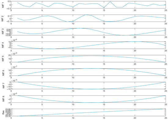
Figure 5. CEEMD decomposition results.

4.4. Comparison and Analysis of Forecast Results

In this paper, nine types of transport carbon emission influencing factors and the measured total transport carbon emissions of Shanghai from 1995 to 2014 are selected as the model-training dataset, and the data from 2015 to 2019 are used as the test set to verify the accuracy of the prediction model. Firstly, the IWOA-KELM model is constructed to each part of each ${imf}_j$ and Res decomposed by the CEEMD technique. The combined prediction results are compared with the IWOA-KELM, WOA-KELM, ELM, BP, LSTM, GRNN, and other models for error comparison. The detailed prediction performance and error results are shown in Figure 6, Figure 7, Figure 8, Figure 9 and Figure 10 and Table 4 and Table 5, based on which the models are further analyzed in depth:

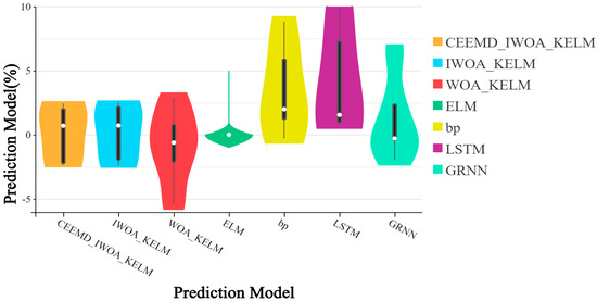
Figure 6. Relative error violin plots for each model.

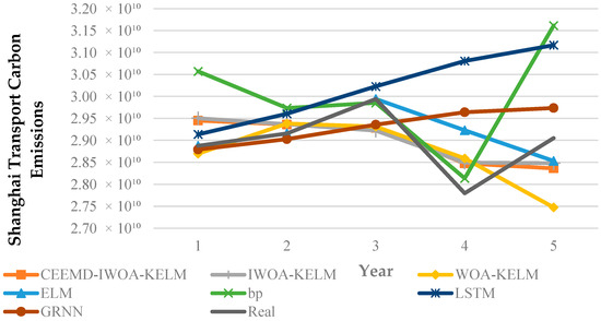
Figure 7. Predicted and real values of Shanghai’s transport carbon emissions by model.

Figure 8. Comparison of MAE and RMSE results for each model.

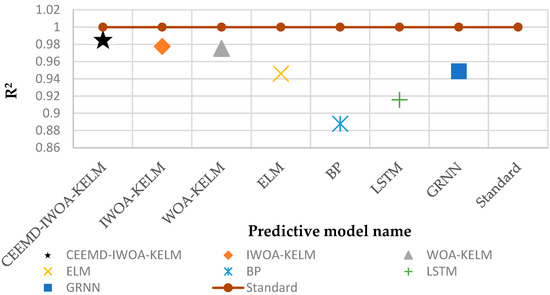
Figure 9. Comparison of R² results for each model.

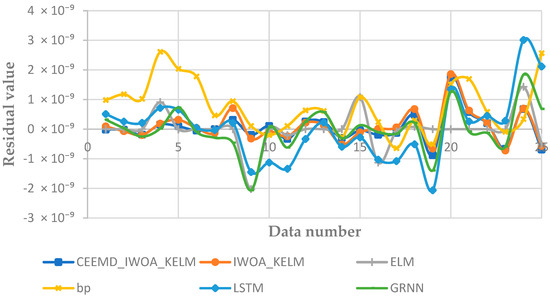
Figure 10. Residual values of each model.

Table 5. Relative error across models.

Year	CEEMD-IWOA-KELM	IWOA-KELM	WOA-KELM	ELM	BP	LSTM	GRNN
2015	2.00%	2.17%	−0.62%	0.00%	5.87%	0.90%	−0.29%
2016	0.70%	0.72%	0.78%	0.00%	1.99%	1.54%	−0.44%
2017	−2.22%	−2.41%	−2.11%	0.00%	−0.30%	0.95%	−1.96%
2018	2.44%	2.51%	2.85%	5.15%	1.22%	10.83%	6.63%
2019	−2.37%	−1.96%	−5.43%	−1.78%	8.82%	7.29%	2.36%

(1)

The analysis of the results presented in Table 5 reveals that the CEEMD-IWOA-KELM prediction model exhibits the highest precision. The analysis of the CEEMD-IWOA-KELM, IWOA-KELM, WOA-KELM, ELM, BP, LSTM, and GRNN models yields the average values of relative errors 0.11%, 0.21%, −0.90%, 0.67%, 3.52%, 4.30%, and 1.26%, and the average relative error of the CEEMD-IWOA-KELM model is 2.44%. The relative error is 2.44%, significantly due to the other models tested.

Figure 6 presents the violin plot depicting the relative errors of the prediction outcomes. The length of the box signifies the degree of data dispersion; a longer box indicates a higher level of dispersion. Upon examination of the figure, it is evident that the CEEMD-IWOA-KELM and IWOA-KELM models have the shortest box lengths. Consequently, these two models display relatively concentrated relative errors.

(2)

Figure 7 shows the predicted and actual values of Shanghai’s transport carbon emissions by model. Compared with the other transport carbon emission prediction models in the test, the CEEMD-IWOA-KELM model shows the best data fitting performance with the highest prediction accuracy, and its predicted trend direction is in high agreement with the dynamic changes in transport carbon emissions in the actual situation.

(3)

Table 6 provides detailed error data. The model proposed in this paper has the highest performance under all four evaluation metrics: RMSE = 0.0324, MAE = 0.0215, MAPE = 0.09%, and R² = 0.9857. Figure 8 combines the MAE and RMSE in a single histogram. It can be clearly seen that the CEEMD-IWOA-KELM model proposed in this paper has the lowest values, indicating the highest model accuracy. Figure 9 displays the R² values of the models. The model closest to the standard line of 1 indicates higher accuracy. It can be observed that the R² value of the CEEMD-IWOA-KELM model is closest to 1.

Table 6. Error simulation results of the prediction models.

Model	RMSE	MAPE	MAE	R2
CEEMD-IWOA-KELM	0.0324	0.0900%	0.0215	0.9857
IWOA-KELM	0.0341	0.1161%	0.0278	0.9820
WOA-KELM	0.0424	0.1243%	0.0297	0.9794
ELM	0.0687	0.2503%	0.0596	0.9302
BP	0.0483	0.1935%	0.0456	0.9386
LSTM	0.0509	0.1900%	0.0449	0.9316
GRNN	0.0687	0.2102%	0.0499	0.8756

(4)

Figure 10 shows the residual values for all predictions made by each model. It can be observed that the CEEMD-IWOA-KELM model and the IWOA-KELM model exhibit a relatively stable performance. In comparison, the BP model shows the poorest stability. The ELM model has some predictions match the actual values closely, but its overall prediction performance is less stable, leading to significant discrepancies. Therefore, using swarm intelligence optimization algorithms to optimize machine learning models is highly necessary.

In summary, from Figure 8, it can be noted that the neutral network model optimized by WOA generally consists of a lower accuracy, and the RMSE of WOA-KELM compared to ELM is improved by 38.24%; the MAPE by 50.35%; the MAE by 50.14%; and the R² by 5.29%, which proves that the swarm intelligence optimization algorithm has a better optimization performance in the neighborhood of transport carbon emissions. IWOA-KELM improves the RMSE by 19.47%; the MAPE by 6.53%; the MAE by 6.56%; and the R² by 0.27% compared to WOA-KELM, which proves that IWOA does obtain an accuracy improvement. CEEMD-IWOA-KELM improves the RMSE by 5.09%; the MAPE by 22.53%; MAE by 22.61%; and R² by 0.38%, proving that CEEMD decomposition can improve the model prediction accuracy. CEEMD-IWOA-KELM compared to ELM shows an improvement in RMSE by 52.79%; in MAPE by 64.05%; in MAE by 63.94%; and in R² by −5.97%, which proves that the proposed CEEMD decomposition can improve the model prediction accuracy based on the individual error. The simulation results prove that the CEEMD-IWOA-KELM model proposed in this paper can significantly improve the model prediction accuracy compared with the ordinary ELM model.

5. Conclusions and Future Work

5.1. Conclusions

In order to solve the volatility and nonlinearity difficulties of transport carbon emission data, this paper constructs the CEEMD-IWOA-KELM model. Firstly, the STIRPAT model is used to screen nine indicators and calculate the total transport carbon emissions of Shanghai; after obtaining the data, CEEMD is used to split the data into several stable internal modal components and residual parts, the mitigated nonlinearities and volatility data sequences are predicted using the IWOA-KELM model, and finally the prediction results of the sequences are merged; finally, all the prediction results are integrated, and from the results of introducing multiple prediction models for comparative analysis, the following conclusions are drawn:

(1)

Effectiveness of data decomposition: The CEEMD technique successfully transformed the transport carbon emission data into a series of low-complexity, smooth components, and this preprocessing step significantly alleviated the nonlinearity and volatility of the original data, and the smooth data can be better used for prediction studies. Compared with the IWOA-KELM model without CEEMD, the average absolute error of the CEEMD-IWOA-KELM model proposed in this paper is reduced by 22.61%, which shows that data decomposition has a significant role in improving prediction accuracy.

(2)

Performance improvement of optimization algorithm: The IWOA algorithm not only maintains the original powerful global search capability of the whale optimization algorithm, but also further improves the prediction accuracy through the quasi-backward learning strategy, the introduction of nonlinear convergence factors, the adaptive weighting strategy, and the stochastic difference variance strategy. The data show that the RMSE value of the IWOA-KELM model is reduced by 19.47% compared with the base WOA-KELM model, and a substantial reduction of 50.26% is achieved compared with the standard ELM model, which clearly proves that the global optimization and generalization ability of the model is significantly enhanced after the optimization of the IWOA and the combination of the kernel function.

5.2. Future Work

(1)

Although the constructed CEEMD-IWOA-KELM model demonstrates significant performance in terms of prediction accuracy, it still faces several challenges. For instance, the factors influencing carbon emissions in the transportation sector are multifaceted, and future research should incorporate more variables to better reflect the actual situation comprehensively. Additionally, the market share of new energy vehicles is increasing year by year, and future studies need to consider the carbon footprint left by new energy vehicles.

(2)

This study primarily focused on the novelty of the model, without delving deeper into predictive analysis. Future work will integrate scenario forecasting to provide a more thorough prediction of carbon emissions in Shanghai’s transportation sector and offer corresponding policies and recommendations. Additionally, the generalizability of the research findings needs attention, considering the extension of the experience in predicting traffic carbon emissions in the Shanghai region to other major cities in China. This would contribute to China’s goal of peaking carbon emissions before 2030 and achieving carbon neutrality before 2060.

References

- Mou, Y.T.; Ke, Z.K. Exploring the scientific consensus on global warming and the misunderstanding of the American public. SIND 2022, 38, 64–70. [Google Scholar]
- Lin, B.; Xie, C. Reduction potential of CO2 emissions in Chinas transport industry. Renew. Sustain. Energy Rev. 2014, 33, 689–700. [Google Scholar] [CrossRef]
- Xi, W.X. Research and analysis of carbon emission influencing factors in Shanghai transportation industry. LEM 2023, 45, 97–100+119. [Google Scholar]
- Wang, Q.R.; Wang, J.J.; Zhu, C.F.; Hao, F. Research on carbon emission prediction of transportation industry by integrating VMD and SSA-LSSVM. Environ. Eng. 2023, 41, 124–132. [Google Scholar]
- Yang, H.; O’Connell, J.F. Short-term carbon emissions forecast for aviation industry in Shanghai. J. Clean. Prod. 2020, 275, 122734. [Google Scholar] [CrossRef]
- Huang, X.Y.; Wu, J.Y.; Lin, W.H.; Wu, Q.X. Carbon emission prediction of Jiangsu Province based on GM (1,1) model. Heilongjiang Sci. 2022, 13, 26–28+32. [Google Scholar]
- Yang, W.L.; Yan, Z.A. Evaluation of CO2 emission from agricultural soils based on RBF neural network algorithm. Softw. Guide 2022, 21, 7–11. [Google Scholar]
- Tursun, B.; Ding, W.M.; Xie, J.H. Neural network-based carbon emission prediction and analysis of influencing factors. Environ. Eng. 2017, 35, 156–160. [Google Scholar]
- Zhang, D.; Wang, T.T.; Zhi, J.H. Carbon emission prediction and eco-economic analysis of Shandong Province based on IPSO-BP neural network model. Ecol. Sci. 2022, 41, 149–158. [Google Scholar]
- Lian, Y.; Su, D.; Shi, S. Carbon Peak Prediction in Fujian Province Based on STIRPAT and CNN-LSTM Combination Model. Environ. Sci. 2024. Available online: https://www.chndoi.org/Resolution/Handler?doi=10.13227/j.hjkx.202401065 (accessed on 5 August 2024). [CrossRef]
- Huang, G.B. An Insight into Extreme Learning Machines: Random Neurons, Random Features and Kernels. Cogn. Comput. 2014, 6, 376–390. [Google Scholar] [CrossRef]
- Zhang, X.S.; Wei, Z.Z.; Chen, Z.Z.; Han, Y.W. Research on industrial carbon emission prediction method based on LASSO-GWO-KELM. Environ. Eng. 2023, 41, 141–149. [Google Scholar]
- Xu, T. Research on Prediction and Classification Based on Swarm Intelligence Algorithm and Machine Learning. Ph.D. Thesis, North China University, Beijing, China, 2021. [Google Scholar]
- Wang, K.; Niu, D.; Zhen, H.; Sun, L.; Xu, X.M. Research on Carbon Emission Prediction in China Based on WOA-ELM Model. Ecol. Econ. 2020, 36, 20–27. [Google Scholar]
- Chi, X.; Xu, Z.; Jia, X.; Zhang, W.J. Carbon Emission Prediction of Power Plants Based on WPD-ISSA-CA-CNN Model. Control. Eng. 2022, 1–8. Available online: https://www.chndoi.org/Resolution/Handler?doi=10.14107/j.cnki.kzgc.20220983 (accessed on 5 August 2024). [CrossRef]
- Long, D. Research on Scenario Prediction of Carbon Emissions in Guangdong Province Based on CSO-FLN. Ph.D. Thesis, North China Electric Power University, Beijing, China, 2022. [Google Scholar]
- Mao, H.S. Carbon emission right price prediction based on CS-BP neural network model. IT&I 2023, 9, 52–55. [Google Scholar]
- Jiao, J.J.; Liu, T.Y. Short-term load forecasting based on ICEEMDAN-IWOA-BiLSTM hybrid algorithm model. Electr. Autom. 2024, 46, 36–39. [Google Scholar]
- Wu, Z.Q.; Mou, Y.M. An improved whale optimization algorithm. Appl. Res. Comput. 2020, 37, 3618–3621. [Google Scholar]
- Bokde, N.D.; Tranberg, B.; Andresen, G.B. Short-term CO2 emissions forecasting based on decomposition approaches and its impact on electricity market scheduling. Appl. Energ. 2021, 281, 116061. [Google Scholar] [CrossRef]
- Zhang, X.S.; Ren, M.Y.; Chen, Z.Z. Research on carbon emission prediction of construction industry based on CEEMD-SSA-ELM method. Ecol. Econ. 2023, 39, 33–39+88. [Google Scholar]
- Cai, B.F.; Zhu, S.L.; Yu, S.M.; Dong, H.M.; Zhang, C.Y.; Wang, C.K.; Zhu, J.H.; Gao, Q.X.; Fang, S.X.; Pan, X.B.; et al. Interpretation of the 2019 Revision of the IPCC 2006 Guidelines for National Greenhouse Gas Inventories. Environ. Eng. 2019, 37, 1–11. [Google Scholar]
- York, R.; Rosa, E.A.; Dietz, T. STIRPAT, IPAT and ImPACT: Analytic tools for unpacking the driving forces of environmental impacts. Ecol. Econ. 2003, 3, 46. [Google Scholar] [CrossRef]
- Liu, J.C. Energy saving potential and carbon emission prediction in China’s transportation sector. Resour. Sci. 2011, 33, 640–646. [Google Scholar]
- Zhu, C.Z.; Yang, S.; Liu, P.B.; Wang, M. Prediction of carbon peaking time in China’s transportation sector. JOTSEIT 2022, 22, 291–299. [Google Scholar]
- Liu, C.; Qu, J.S.; Ge, Y.J.; Tang, J.X.; Gao, X.Y.; Liu, L.N. Carbon emission prediction of China’s transportation industry based on LSTM model. China Environ. Sci. 2023, 43, 2574–2582. [Google Scholar]
- Wang, Y.; Hayashi, Y.; Kato, H.; Liu, C. Decomposition analysis of CO2 emissions increase from the passenger transport sector in Shanghai, China. Int. J. Urban Sci. 2011, 15, 121–136. [Google Scholar] [CrossRef]
- Hu, M.F.; Zheng, Y.B.; Li, Y.H. Prediction of peak carbon emissions from transportation in Hubei Province under multiple scenarios. CST 2022, 42, 464–472. [Google Scholar]
- Loo, B.P.Y.; Li, L. Carbon dioxide emissions from passenger transport in China since 1949: Implications for developing sustainable transport. Energy Policy 2012, 50, 464–476. [Google Scholar] [CrossRef]
- Timilsina, G.R.; Shrestha, A. Transport sector CO2 emissions growth in Asia: Underlying factors and policy options. Energy Policy 2009, 37, 4523–4539. [Google Scholar] [CrossRef]
- Zhang, H.; Kong, X.; Ren, C.X. Influencing factors and forecast of carbon emissions from transportation-taking Shandong province as an example. EES 2019, 300, 032063. [Google Scholar] [CrossRef]
- Yang, S.H.; Zhang, Y.Q.; Geng, Y. Analysis of transportation carbon emission changes in the Yangtze River Economic Belt based on LMDI. China Environ. Sci. 2022, 42, 4817–4826. [Google Scholar]
- Zhou, Y.X. Research on the decoupling and coupling relationship between transportation carbon emissions and industry economic growth—Based on Tapio decoupling model and cointegration theory. Inq. Into Econ. Issues 2016, 407, 41–48. [Google Scholar]
- Fan, Y.J.; Qu, J.S.; Zhang, H.F.; Xu, L.; Bai, J.; Wu, J.J. Research on the current situation and influencing factors of transportation carbon emissions in five provinces and regions in Northwest China. Ecol. Econ. 2019, 35, 32–37+67. [Google Scholar]
- Huang, N.E.; Shen, Z.; Long, S.R.; Wu, M.C.; Shih, H.H.; Zheng, Q.; Yen, N.C.; Tung, C.C.; Liu, H.H. The empirical mode decomposition and the Hilbert spectrum for nonlinear and nonstationary time series analysis. Proc. R. Soc. A-Math. Phys. 1998, 454, 903–995. [Google Scholar] [CrossRef]
- Wu, Z.H.; Huang, N.E. Ensemble empirical mode decomposition: A noise-assisted data analysis method. Adv. Adapt. Data Anal. 2009, 1, 1–41. [Google Scholar] [CrossRef]
- Yeh, J.R.; Shieh, J.S.; Huang, N.E. Complementary ensemble empirical mode decomposition: A novel noise enhanced data analysis method. Adv. Adapt. Data Anal. 2010, 2, 135–156. [Google Scholar] [CrossRef]
- Mirjalili, S.; Lewis, A. The Whale Optimization Algorithm. Adv. Eng. Softw. 2016, 95, 51–67. [Google Scholar] [CrossRef]
- Huang, G.B.; Zhu, Q.Y.; Siew, C.K. Extreme learning machine: Theory and applications. Neurocomputing 2006, 70, 489–501. [Google Scholar] [CrossRef]
- Chen, L.; Hao, Y.C.; Li, Q.R.; Ding, J.X. Improved BP neural network traffic prediction model for SSA optimization. JHIT 2024, 56, 1–10. [Google Scholar]
- Chen, H.W.; Xing, W.W.; Zhao, C.L.; Cao, B.H.; Liu, J.H.; Zhao, X.H.; Yang, L.W. Prediction of N2O emission from wastewater treatment plant based on CEEMDAN-LSTM model. Water Wastewater Eng. 2024, 60, 166–172. [Google Scholar]
- Zhou, J.G.; Zhang, M. Combined NOx emission prediction for thermal power industry based on improved gray and generalized neural network. Environ. Eng. 2014, 32, 120–125. [Google Scholar]
Disclaimer/Publisher’s Note: The statements, opinions and data contained in all publications are solely those of the individual author(s) and contributor(s) and not of MDPI and/or the editor(s). MDPI and/or the editor(s) disclaim responsibility for any injury to people or property resulting from any ideas, methods, instructions or products referred to in the content. |
© 2024 by the authors. Licensee MDPI, Basel, Switzerland. This article is an open access article distributed under the terms and conditions of the Creative Commons Attribution (CC BY) license (https://creativecommons.org/licenses/by/4.0/).