An Analysis of the Energy Consumption Forecasting Problem in Smart Buildings Using LSTM

Abstract

This work explores the process of predicting energy consumption in smart buildings based on the consumption of devices and appliances. Particularly, this work studies the process of data analysis and generation of prediction models of energy consumption in Smart Buildings. Specifically, this article defines a feature engineering approach to analyze the energy consumption variables of buildings. Thus, it presents a detailed analysis of the process to build prediction models based on time series, using real energy consumption data. According to this approach, the relationships between variables are analyzed, thanks to techniques such as Pearson and Spearman correlations and Multiple Linear Regression models. From the results obtained with these, an extraction of characteristics is carried out with the Principal Component Analysis (PCA) technique. On the other hand, the relationship of each variable with itself over time is analyzed, with techniques such as autocorrelation (simple and partial), and Autoregressive Integrated Moving Average (ARIMA) models, which help to determine the time window to generate prediction models. Finally, prediction models are generated using the Long Short-Term Memory (LSTM) neural network technique, taking into account that we are working with time series. This technique is useful for generating predictive models due to its architecture and long-term memory, which allow it to handle time series very well. The generation of prediction models is organized into three groups, differentiated by the variables that are considered as descriptors in each of them. Evaluation metrics, RMSE, MAPE, and R² are used. Finally, the results of LSTM are compared with other techniques in different datasets.

1. Introduction

This section discusses the need for energy consumption forecasting models in the context of building energy management systems. In addition, the novelty and contributions of this research are presented.

1.1. Motivation

One of the main current challenges is the efficient consumption of energy due to economic and environmental reasons, among others. The massive energy consumption entails more economic expenses, impact on the environment, etc. However, thanks to the evolution of technology, it is possible to develop smart energy management systems (SEMSs) that efficiently save energy, without degrading user comfort. In this context, the application of soft computing techniques is necessary.

On the other hand, the building sector consumes more energy than the industry and transportation sectors, which is due mainly to Heating, Ventilation, and Air Conditioning (HVAC) systems, appliances/devices, and lighting [1,2]. Particularly, it is interesting to analyze the appliances/devices consumption in the context of a SEMS for several reasons, e.g., to minimize the utilization of the energy when the prices are excessive to guarantee the comfort to the users, or to have a sustainable rate of consumption considering the environment.

A smart building is a dynamic system where technology is used to improve its functioning, considering hundreds of elements, such as its HVAC system, appliances and devices, etc. In this context, SEMS must seek energy efficiency, implementing energy management tasks, such as monitoring of energy supply, predicting energy consumption, and anomaly detecting of energy use, among others.

Thus, among the possible reasons to analyze the energy consumption in smart buildings are the following: to determine the electrical load; to detect anomalies in consumption; to estimate energy consumption; to define load profiles using consumption behavior; and to classify the consumers, among others. In this way, to reach optimal management of energy consumption in a smart building, it is necessary to study the consumption, which is precisely the scope of this paper. Thereby, possible energy problems can be detected and solved. At the same time, around a smart grid, the energy is intermittent, distributed, mobile, and able to be stored. For example, renewable energy resources (RES) are characterized by their variability and intermittency, which make the prediction of the generated energy complex [1,2]. These attributes make the implementation of SEMSs more challenging, because more flexibility and stability is needed to secure its normal operation in a building, for which efficient energy consumption forecasting models are required. SEMSs today do not consider these aspects for this highly complex and rapidly changing scenario.

On the other hand, Artificial Intelligence (AI) can build useful knowledge of factors such as the prediction of energy consumption and the prediction of occupancy behavior, among others. AI techniques are already being used in the SEMSs, such as tasks of modeling, learning, and reasoning, among others. The motivation of this work is to analyze the behavior of the energy consumption data of the devices and electrical appliances in a building, in order to build models that allow prediction of their behavior.

1.2. Background

In the literature, there are some works similar to this work. For example, Rodriguez-Mier et al. [3] proposed a knowledge model to define predictive models of energy consumption for smart buildings, and a multi-step prediction model based on a hybrid genetic-fuzzy system, which includes a feature selection method. The authors use a database that stores two types of signals: synchronous signals that record at a constant rate of 10 s (e.g., temperature, sensors, etc.) and asynchronous signals that record when a value changes (e.g., the indoor temperatures, error signals, etc.). In addition, they collect the humidity, solar radiation power, and pressure. Garcia et al. [4] present a comparative study of different forecasting strategies of the energy consumption of smart buildings. Particularly, they determine that strategies based on Machine Learning (ML) approaches are more suitable. Alduailij et al. [5] analyze several statistical and ML techniques to predict energy consumption for five different building types. They especially predict the peak demand that serves to achieve energy efficiency. Hernández et al. [6] present an energy consumption forecasting strategy that allows hourly day-ahead predictions using several ML techniques. Then, they define an ensemble model using the mean of the prediction values of the top five models. In addition, Hernández et al. [7] present a review of energy consumption forecasting for improving energy efficiency in smart buildings. They analyze different forecasting methods in nonresidential and residential buildings in terms of forecasting methods, forecasting objectives, input variables, and prediction horizon.

Moreno et al. [8] define predictive models of energy consumption and save energy for buildings based on the Radial Basis Function (RBF) technique. Nabavi et al. [9] propose a Deep Learning (DL) method that uses a discrete wavelet transformation and the long short-term memory method to forecast building energy demand and energy supply. These methods consider several factors, such as energy consumption patterns in buildings, electricity price, availability of renewable energy sources, and uncertainty in climatic factors. Somu et al. [10] present an energy consumption forecasting model which employs LSTM. The hyperparameter optimization process (learning rate, number of layers, momentum, and weight decay) of the LSTM was optimized using the sine–cosine optimization algorithm.

On the other hand, Le et al. [11] develop a framework for multiple energy consumption forecasting of a smart building based on the use of the Transfer Learning concept. Hadri et al. [12] implement different energy consumption forecasting approaches of appliances by integrating the occupancy and the context-driven control information of buildings. In addition, Gonzalez-Vidal et al. [13] defined a methodology to transform the multivariate time-dependent series to be used by ML algorithms for energy forecasting. Then, González-Vidal et al. [14] proposed ML and grey-box approaches to predict energy consumption based on the physics of the building’s heat transfer. Sulo et al. [15] analyzed the ways to improve the efficiency of the energy used by buildings using an LSTM model to predict the energy consumption of the buildings on the campuses of the City University of New York.

In other contexts, Aliberti et al. [16] proposed a predictive model to estimate the indoor air temperature in individual rooms with a prediction window of up to three hours, and for the whole building with a prediction window of four hours. In addition, Lawadi et al. [17] compared several ML algorithms to estimate the indoor temperature in a building, which were evaluated using different metrics, such as accuracy and robustness to weather changes. Siddiqui et al. [18] introduced a DL approach to recommend consumption patterns for the appliances based on Term Frequency–Inverse Document Frequency (TF-IDF) to quantify the energy tags. The aim of the work of Bhatt et al. [19] was to forecast the cost of energy consumption in smart buildings. They proposed a balanced DL algorithm that considers three constraints to solve the price management problem and high-level energy consumption in HVAC systems [20]. Bourhnane et al. [21] used Artificial Neural Networks (ANN) along with Genetic Algorithms (GA) to define an approach for energy consumption prediction and scheduling.

The motivation of the work of Hadri et al. [22] was to determine the forecasting quality and the computational time of the XGBOOST, LSTM, and SARIMA algorithms in the context of forecasting energy consumption. Khan et al. [23] proposed a short-term electric consumption forecasting model based on spatial and temporal ensemble forecasting. The ensemble forecasting model consists of a K-means algorithm to determine energy consumption profiles, and two deep learning models, LSTM and Gated Recurrent Unit (GRU). The model forecasts the energy consumption at three spatial scales (apartment, building, and floor level) for hourly, daily, and weekly forecasting horizons. The work of Keytingan et al. [24] proposed predictive models for energy consumption based on a Support Vector Machine, Artificial Neural Networks, and K-Nearest Neighbour using real-life data of a commercial building from Malaysia. The goal of the work of Son et al. [25] was to study adaptive energy consumption forecasting models in order to follow the dynamics of buildings. They consider active and passive change detection methods, which are integrated into the decision tree and deep learning models. The results showed that constant retraining, in some cases, is not good in performance. Moon et al. [26] proposed an online learning approach to enable fast learning of building energy consumption patterns for unseen data. In addition, Pinto et al. [27] presented three ensemble learning models (XGBOOST, random forests, and an adaptation of Adaboost) for energy consumption forecasting an hour ahead, using real data from an office building. Finally, the work of Somu et al. [28] described a deep learning framework based on CNN (Convolutional Neural Networks)-LSTM to provide building energy consumption forecasts. CNN-LSTM uses K-means to determine the energy consumption pattern/trend, CNN to extract features about energy consumption, and LSTM to handle long-term dependencies.

In summary, the vast majority of recent works have been dedicated to carrying out comparative studies of different building energy consumption forecasting strategies based on statistical and ML techniques for different types of buildings (residential, office, among others), using specific datasets [4,5,6,7,8,16,17,18,19,22,24,27]. In some of these comparisons, specific aspects have been analyzed, such as occupation [12], how to follow the dynamics of energy consumption [25], or the use of online learning approaches to follow the consumption pattern in real time [26]. On the other hand, some works analyzed the relationships of temporal dependencies in the time series in order to forecast the energy demand and/or the energy supply of the building [9,10,14,23], and in some cases, use the LSTM model [15,28] or feature selection methods [3,28] to predict energy consumption in buildings. Other works have studied the Transfer Learning concept in the context of forecasting the energy consumption of intelligent buildings [11], or have combined it with other techniques to consider the prediction and programming of energy consumption [20].

In conclusion, there are many works on the prediction of energy consumption in smart buildings, but none of them propose a scheme to carry out an exhaustive feature engineering process to analyze the variables, their dependencies, and their transformations, which allows improvement of the prediction of the forecasting models. Specifically, the great gap in the previous works is that they do not propose strategies to analyze the implicit temporal relationships in the time series that describe the pattern of energy consumption, which affects/degrades the ML and the statistical algorithms used to build the models of forecasting of energy consumption.

1.3. Novelty and Our Contribution

This work studies the process of data analysis and generation of prediction models of energy consumption in smart buildings. The focus of this paper is to estimate energy consumption in smart buildings based on the consumption of the appliances and devices in them. Therefore, thanks to the data collected in smart buildings, the study is carried out on this energy consumption as a function of time, in order to obtain a model capable of estimating total consumption, knowing the consumption of the devices and appliances in the building. The reason for working with time series is that energy consumption can be labeled by times of the year, days of the week, or even hours on the same day. For example, at Christmas, there may be a greater consumption of Christmas lights, and in holiday months, the consumption may be lower if we are traveling. The research question is whether the prediction of energy consumption in a building depends on an exhaustive analysis of time series that describe its behavior, which would imply carrying out a specific feature engineering process for that context.

This work carries out an analysis of these variables and their relationships, thanks to techniques such as the Pearson and Spearman correlations, and Multiple Linear Regression models. With the results obtained, the fusion and extraction of characteristics are carried out with the Principal Component Analysis (PCA) technique. On the other hand, the relationship of each variable with itself over time is analyzed, using techniques such as autocorrelation (simple and partial) and ARIMA models. Finally, several forecasting models are generated with LSTM. We start from the hypothesis that LSTM is an excellent technique for treating time series [29,30], so we have chosen this technique to analyze the results of our feature engineering process. With these results, the generation of prediction models is organized into three groups. The first group consists of prediction models in which only the first Principal Component (PC1) is taken into account. The second group includes PC2. The last group uses the original variables. These groups of models are evaluated using the following metrics: Root Mean Square Error (RMSE), Mean Absolute Percentage Error (MAPE), and R². Thus, the main contribution of this article is the definition of a feature engineering methodological approach to analyze the energy consumption variables of buildings. Other specific contributions derived from that contribution are:

• The definition of the phases to study the time series that define energy consumption in buildings;
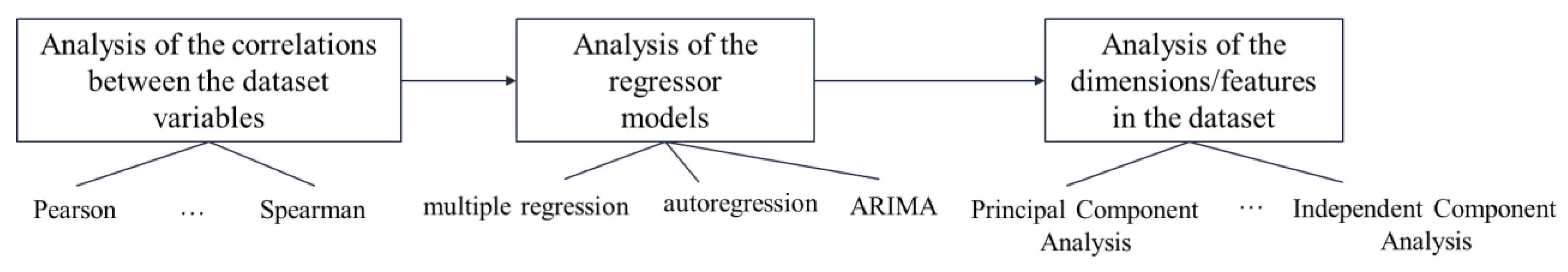
• The definition of the analysis process of the dependency relations between the variables, especially the temporal ones;
• The definition of the analysis process of the dimensions in the dataset to determine the fusion and extraction of characteristics.
• The utilization of this approach for the definition of forecast models based on time series.

The remainder of this work is organized as follows. A preliminary theoretical framework is described in Section 2. The analysis of the energy forecasting problem is reported in Section 3 based on two aspects. It begins by defining our feature engineering approach for energy consumption time series, then describes its detailed application in a case study, and finally builds a forecast model using LSTM from the results obtained with it. Section 4 presents a comparison of LSTM with other machine learning techniques in different time series on building energy consumption, using our feature engineering approach to define the forecast model. Finally, a discussion about future directions in this domain is pointed out in Section 5.

2. Theoretical Framework

In this section, we formalize the problem of energy consumption forecasting in smart buildings and present the ML technique used for the forecasting task.

2.1. The Energy Consumption Forecasting Problem

Particularly, the energy consumed by the ‘n’ elements in a building (e.g., an HVAC system, an electrical appliance) has a timestamp t, recorded by the sensors deployed in the building, and can be described as [10]:

$$X_t=\left\{x_{1t},x_{1t}, \dots , x_{1nt} \right\}$$

where x_it is the energy consumption captured by the ith sensor at tth timestamp, and n is the number of sensors. Normally, the data-driven forecasting models use a window-based approach for forecasting, defined by two variables, the input window (I_w) and the forecast window (F_w) sizes. Thus, the total number of inputs and forecasts is defined in [10] as $k=\left(S_n-I_w-a\right)/F_w$, where a is the forecast interval and S_n is the total number of samples.

Subsequently, the input (S_I) of size I_w is S_I = {X_t, X_t+1, …, X_t+k}. Similarly, the forecast (S_F) of size F_w is {$S_F=\widehat{\{X_t,}\widehat{X_{t+1}}, \dots , \widehat{X_{t+k}}\}$.

Therefore, a non-linear approximation function (f) can be defined as S_F = f(S_I). Hence, for a given time window (I_w), the model (f) learns to forecast their values for the time window (F_w) with minimal forecast error between the actual and forecasted energy consumption value of the sensors at each timestamp. The input window and forecast window sizes can be adjusted according to the forecast problem (long-term, mid-term, and short-term memory).

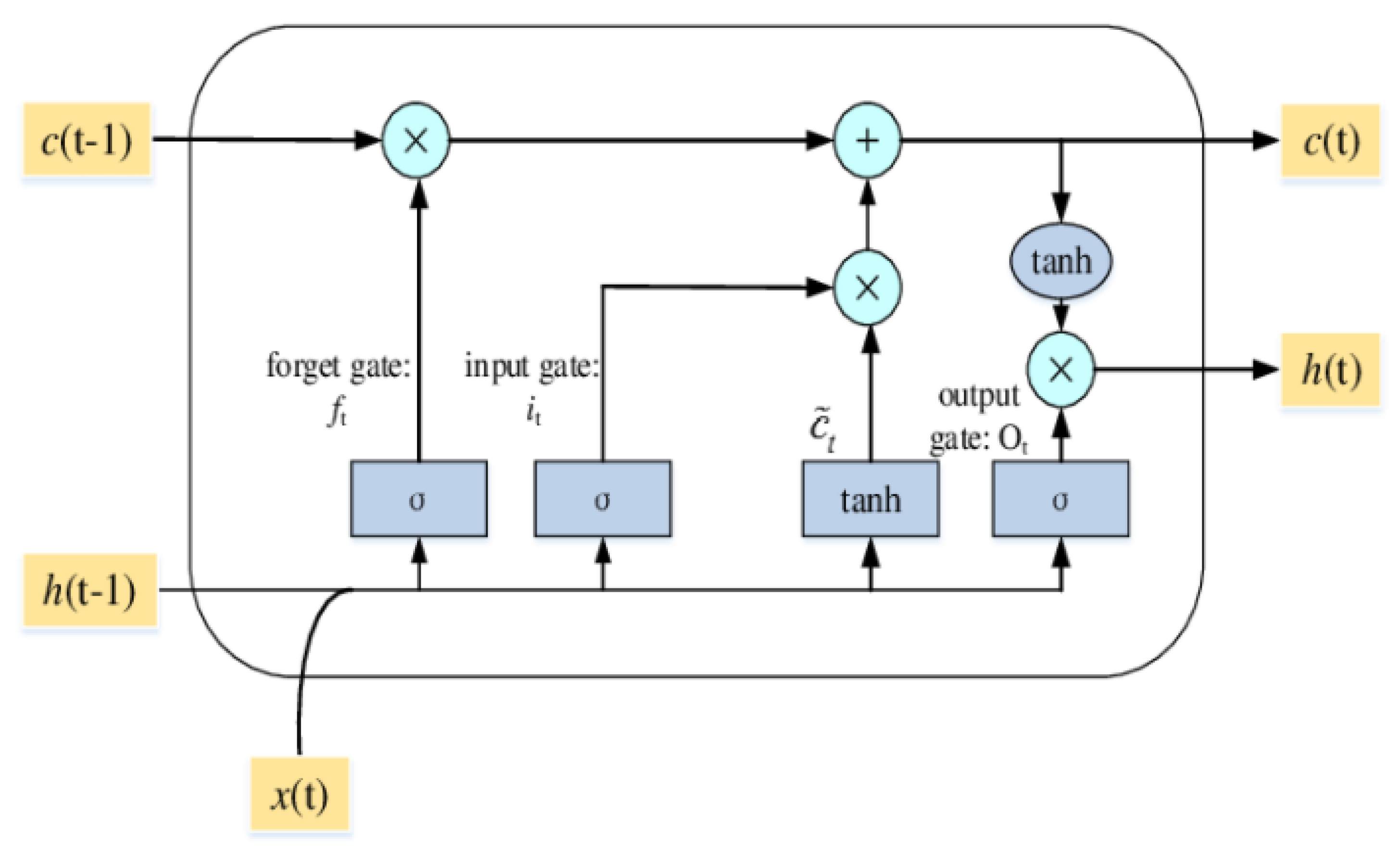
2.2. Long Short-Term Memory (LSTM) Technique

Long Short-Term Memory (LSTM) technique is a type of Recurrent Neural Network (RNN). The RNNs [30], unlike traditional neural networks, are capable of processing data sequences, that is, data that need to be interpreted together in a specific order to have meaning. This is possible thanks to the fact that the RNNs have an architecture that allows them, at each instant of time, to receive the input corresponding to that instant, in addition to the value of the activation in the previous instant. These previous instants of time allow a certain “memory”, since they retain the information from previous steps. Thus, they have a memory cell that preserves the state over time. In addition, the RNNs apply backpropagation through time (BPTT).

However, the “memory” of traditional RRNs is a short-term memory, since, as the information is transmitted through time, the effect of the state of an instant will be very small at a very distant instant. Given this drawback, the LSTM [29,30] emerged. These networks are capable of maintaining information both in the short and long term, thanks to the incorporation of the cell state (c). The cell state c encodes the information of the inputs (relevant info) that have been observed up to that step. This cell state is updated according to the current state of the cell, the output at time t−1, the input at time t, and a series of gates that are responsible for processing this information. The gates are the following:

A forget gate that, receiving input x at time t and output h at time t−1, decides what information will be discarded; that is, it will not be part of the state for that instant.

An update gate (or input gate) that determines what information in the cell state c to update from the input x at time t and the output h at time t−1.

An output gate, which will generate the output h for the instant t from the information in the cell state c. However, not all of the information from the cell state is dumped in the output; instead, a selection is made of the information of the cell state that has been considered important to use at the next time.

Figure 1 shows the architecture of an LSTM network, with each of the parts explained above [29,30].

In this way, the behavior of an LSTM neural network tries to replicate human learning. To process information that requires long-term memory, we do not keep all the data, but only the most relevant, which will be useful to understand what we are dealing with. This ability of LSTM networks to retain information in the long term, makes this type of network the ideal option to create the prediction models in our work. This is because the time series of energy consumption are correlated with values in past time intervals, which can be days, but can also be weeks, months, or years. For example, in the context of energy consumption of devices, the following case may occur: if we want to predict the total consumption on Mondays, the forget gate will be in charge of discarding the information on the consumption of the devices of the last Wednesday, because it is not relevant. On the other hand, the update gate will add data on the consumption of the devices for Mondays, since this information is useful for predicting the total consumption of that day. In this way, the output gate could determine the total consumption for Monday by combining the input data with the selected data from the cell state, such as the consumption of last Monday.

3. Analysis of the Energy Consumption Forecasting Problem

This section presents a deep analysis of the Energy Consumption Forecasting Problem. It is divided into three subsections. The first carries out a feature engineering process to obtain the variables to be used in the predictive models. This process analyzes the variables of the dataset to determine their quality, their correlations and autocorrelations, and the selection and fusion of variables, among other things. The next subsection describes the generation of energy consumption prediction models using the LSTM technique. Particularly, an initial general predictive model is generated, from which three groups of models are created according to the descriptive variables selected by the feature engineering process. In the third subsection, a comparison is made between the models of each group.

3.1. Analysis of the Variables (Feature Engineering Process)

This section presents the feature engineering process proposed in this work to analyze the energy consumption in smart buildings (see Figure 2).

Figure 2 shows that there are 3 major processes: (i) analysis of the correlations between the variables; (ii) analysis of regressive models; (iii) analysis of the dimensions. In the first case, the different types of correlations, linear or not (Pearson and Spearman, among others), between the variables and with the target variable (in our case, the energy consumption) are analyzed. In particular, the variables that are not correlated with the objective variable to be estimated are eliminated, or one of the variables that has a high correlation between them is chosen in order to avoid the collinearity problem. Regarding the second case, since it is a forecast model, its different forms are analyzed by studying the possible combinations between the variable of interest and all of the predictor variables (multiple regression model), or the regression of the variable against itself (autoregression or ARIMA models, among others). Finally, the last phase creates an analysis of the dimensions/characteristics in the dataset to determine if they can be reduced (Principal Component Analysis) or extract information of interest (Independent Component Analysis), among other possible studies.

Next, in this section, we explain this feature engineering process in detail for a dataset about the energy consumption in a building. The dataset used is Raw_Data.csv [31], which is a time-series of the energy consumption of the Research Support Facility (RSF) building of the United States National Renewable Energy Laboratory. It has 34 attributes, some of which are:

• Date: represents the date each sample is taken, with the format: YYYY: MM: DD.
• Month: represents the month in which each sample is taken (integer).
• Day: represents the day of the week (Sunday–Monday) on which each sample is taken (string).
• Time: represents the time of day at which the sample is taken, with the format hh: mm (time).
• Hour and Minute: represent the hour and minute of the sample collection, respectively (integer).
• Skyspark: represents the total energy consumption for each observation, in kilowatts (kW). This will be the target or dependent variable.
• AV.Controller, Coffee.Maker, Copier, Office Computer, Lamp, Laptop, Microwave, Monitor, Phone.Charger, Printer, Projector, Toaster.Oven, TV, Video.Conference.Camera, Water.Boiler, Conference.Podium, Auto.Door.Opener, Treadmill, Refrigerator, Central-Monitoring-Station, TVs, etc. represent the energy consumption of each device in each observation (kilowatts (kW)). These will be our descriptive or independent variables.

This data set has 26,496 observations, collected every 5 min, from 1 October 2019 at 00:00 to 31 December 2019 at 23:55. Additionally, the variables Month, Day, Hour, and Minute are not necessary to keep them, since this information is condensed in the variable Date_Time. This variable will be set as the index (timestamp). It can also be observed that some columns do not provide information, since all their values are 0 (e.g., the variables Conference.Podium, Central.Monitoring.Station, and Auto.Door.Opener, among others). Therefore, they are eliminated.

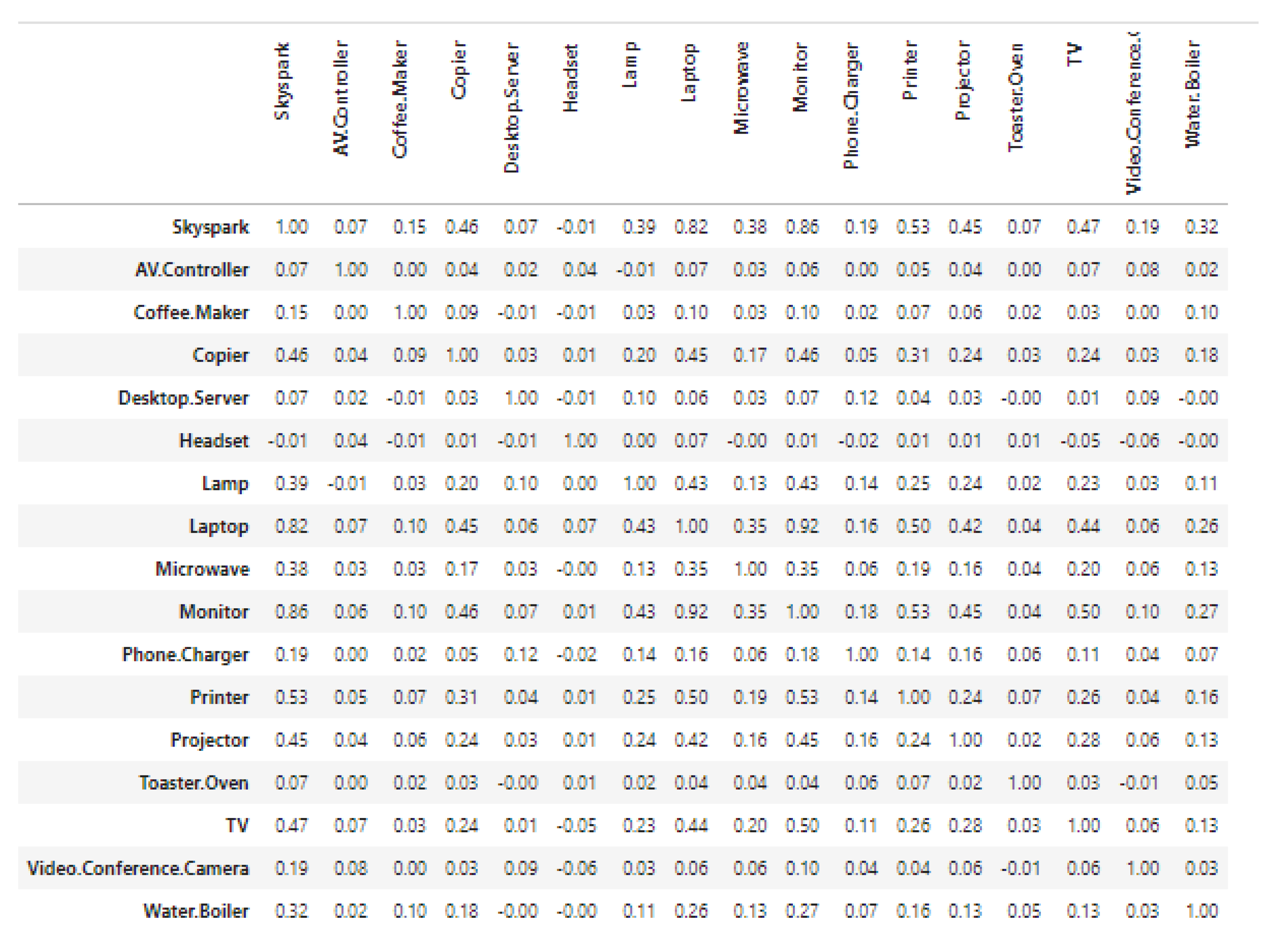
3.1.1. Analysis Using Pearson’s Correlation

In order to analyze the existence of linear relationships, the Pearson correlation coefficients between each pair of variables are used. Figure 3 shows these results.

According to the literature, Pearson correlations between variables less than 0.2 indicate that there is little relationship between them, while correlations greater than 0.8 indicate that there are high correlations between them [3,13,32]. In Figure 2, the Pearson correlation coefficients between the Skyspark variable and the following descriptor variables are less than 0.2: AV.Controller: 0.07, Coffee.Maker: 0.15, Desktop.Server: 0.07, Headset: −0.01, Phone.Charger: 0.19, Toaster.Oven: 0.07, Video.Conference.Camera: 0.19. This means that these variables are very poorly correlated with the target variable. They do not provide relevant information for the generation of a predictive model of the Skyspark variable. Therefore, they can be deleted.

On the other hand, the following pairs of variables have a coefficient greater than 0.8: Skyspark–Laptop: 0.82, Skyspark–Monitor: 0.86 and Laptop–Monitor: 0.92. The descriptor variables Laptop and Monitor are highly correlated with each other. Furthermore, these same variables are, in turn, highly correlated with the target variable. This can negatively affect the modeling, so it will be analyzed later.

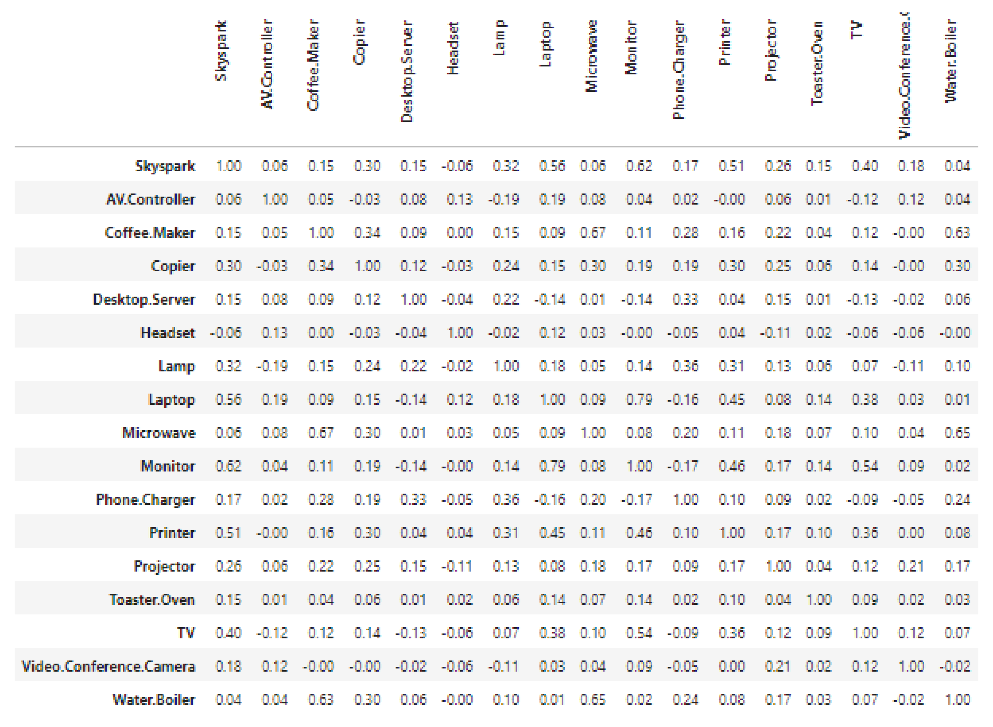
3.1.2. Analysis Using Spearman’s Correlation

In addition to analyzing the linear relationships between the variables, it is necessary to analyze the non-linear relationships. Thus, the Spearman correlation coefficients are determined (see Figure 4).

The most significant correlations are between the following variables: Laptop–Monitor: 0.79, Coffee.Maker–Microwave: 0.67, Microwave–Water.Boiler: 0.65. In this case, it is observed that there is a non-linear correlation between two pairs of variables that were not linearly related (Coffee.Maker–Microwave and Microwave–Water.Boiler). However, a high coefficient is also obtained for the Laptop and Monitor variables, thus confirming that these two variables are mutually correlated. Furthermore, the variables that had a weak linear correlation with the target variable (Skyspark) also have a weak non-linear correlation (AV.Controller, Coffee.Maker, Desktop.Server, Headset, Microwave, Phone.Charger, Toaster.Oven, Video.Conference.Camera, and Water.Boiler). The variables that are not correlated with Skyspark can be eliminated. On the other hand, for the descriptive variables that are highly correlated with each other (Laptop and Monitor), there are two options. The first one consists of selecting one of the variables, thus eliminating the redundant information that this correlation supposes. The second option consists of carrying out an extraction/fusion of characteristics, so that we obtain new variables, which have information about each of the original variables, without being correlated between them. In order to do this, we apply a Principal Component Analysis (PCA).

3.1.3. Analysis Using Multiple Linear Regression

Another technique used to analyze linear relationships between variables is the generation of Multiple Linear Regression models. In this case, we generate a model for each descriptor variable in order to detect possible collinearities. That is, for each descriptor variable, there is a model in which it is the dependent variable and the other descriptor variables are independent variables.

Table 1. Multiple Linear Regression Models.

Model	R2	p-Value
AV.Controller	0.019	2.99 × 1099
Coffee.Maker	0.020	3.62 × 10106
Copier	0.230	0.00
Desktop.Server	0.031	8.48 × 10174
Headset	0.031	1.69 × 10173
Lamp	0.205	0.00
Laptop	0.848	0.00
Microwave	0.132	0.00
Monitor	0.867	0.00
Phone.Charger	0.063	0.00
Printer	0.297	0.00
Projector	0.214	0.00
Toaster.Oven	0.010	2.90 × 1050
TV	0.262	0.00
Video.Conference.Camera	0.036	8.81 × 10199
Water.Boiler	0.086	0.00

shows R² and the p-value for each model generated.

Table 1 shows that there are two models with a very high R² (for the variables Laptop and Monitor), with a value of 0.848 and 0.867, respectively. In addition, the p-value for these models is less than 0.05. These results indicate that these variables have a fairly strong linear relationship with at least one of the other descriptor variables. This coincides with the results of Pearson’s correlation, where it was seen that a linear relationship exists between these two variables.

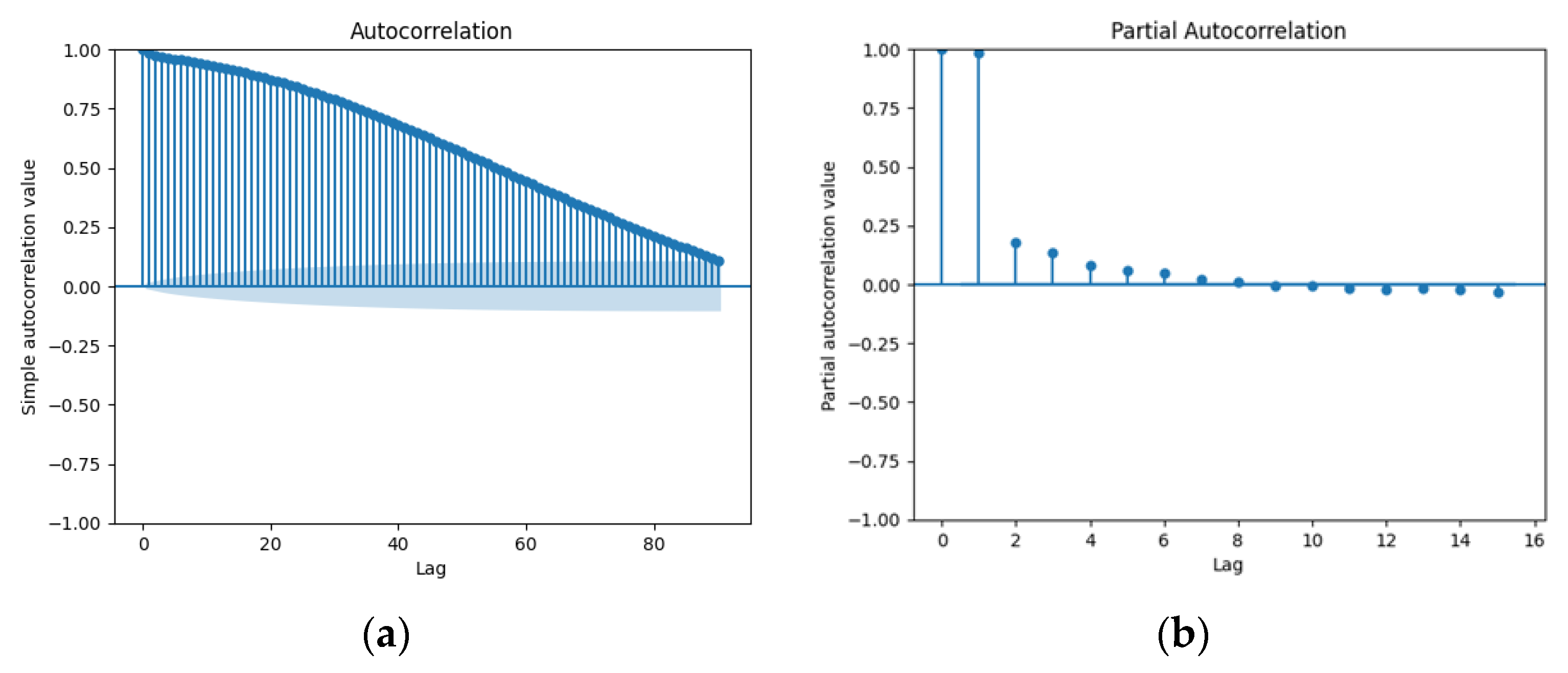
3.1.4. Autocorrelation Analysis

The autocorrelation determines how many previous instants of time affect the energy consumption of a given observation. This number, known as time delay or lag, is required by the LSTM technique. Simple autocorrelation and partial autocorrelation of the target variable (Skyspark) are shown in Figure 5. The x-axis represents the lags, and the y-axis represents the autocorrelation value.

According to the simple autocorrelation (Figure 5a), the limit of the confidence interval of 0.05 is at lag 90. This means that the first 90 lags are statistically significant and, therefore, directly or indirectly influence the energy consumption values for each observation. On the other hand, the partial autocorrelation indicates that only seven lags are statistically significant (Figure 5b). That is, only six previous instants produce a direct effect on the values of a given observation. However, the utility of simple and partial correlations is that they are used to obtain ARIMA models. This is because the delay obtained from the simple autocorrelation corresponds to the parameter q of the ARIMA models, while the delay obtained from the partial autocorrelation corresponds to the parameter p (see Section 3.1.6 where there is an introduction to ARIMA models).

In this way, from an initial model created with these values, new models can be adjusted to find the most accurate one. With this last adjusted model, the time window to be used in our LSTM models will be established later. For example, the ARIMA model which starts the fit would be ARIMA (90, 0, 6). The parameter d is 0 because the time series in the Skyspark variable is non-stationary; that is, there is a trend or seasonality. This is shown in Figure 6, where there is a representation of the values of the Skyspark variable over time (first Figure), and their decomposition into trend, seasonality, and residuals, respectively.

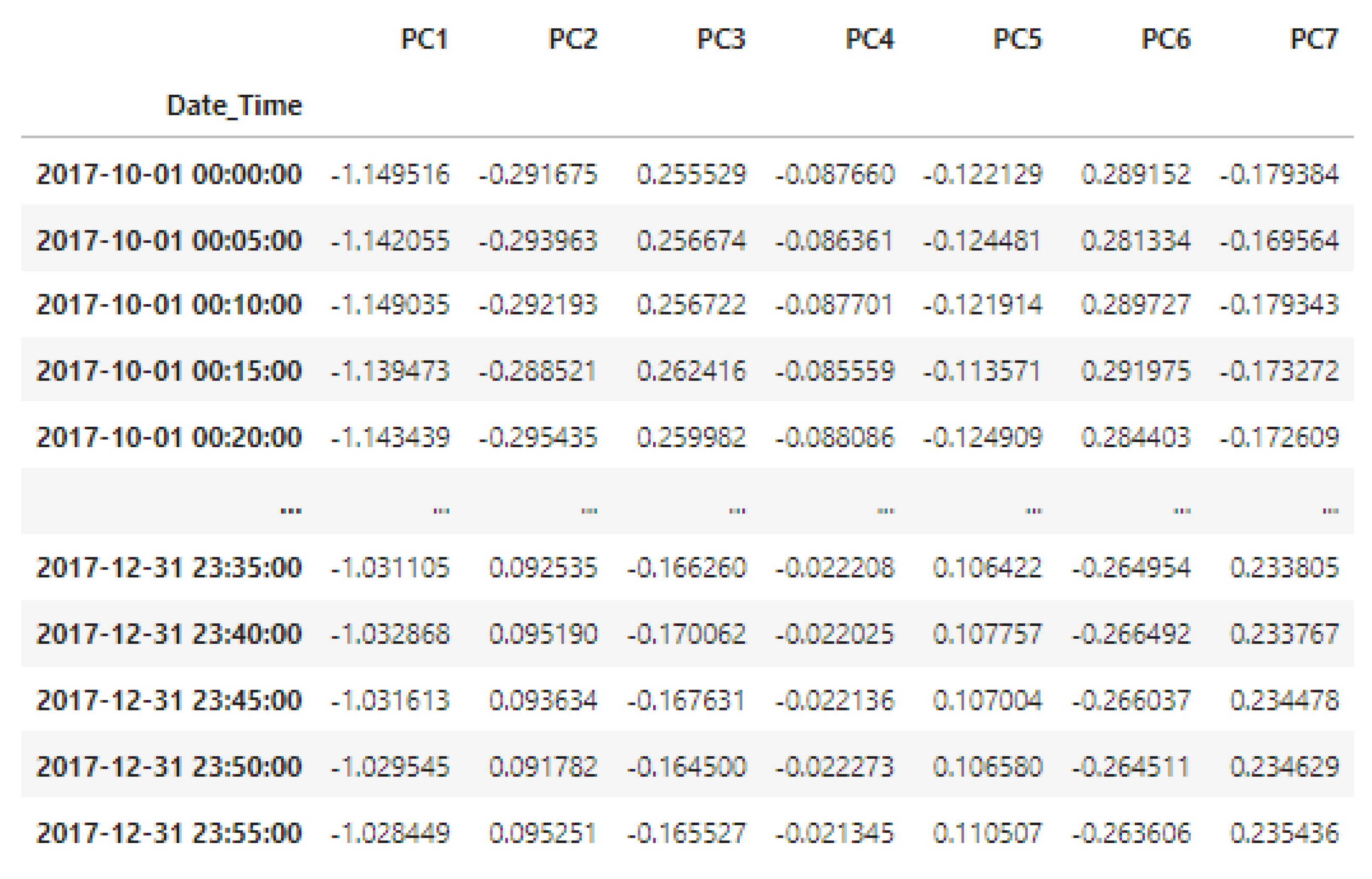
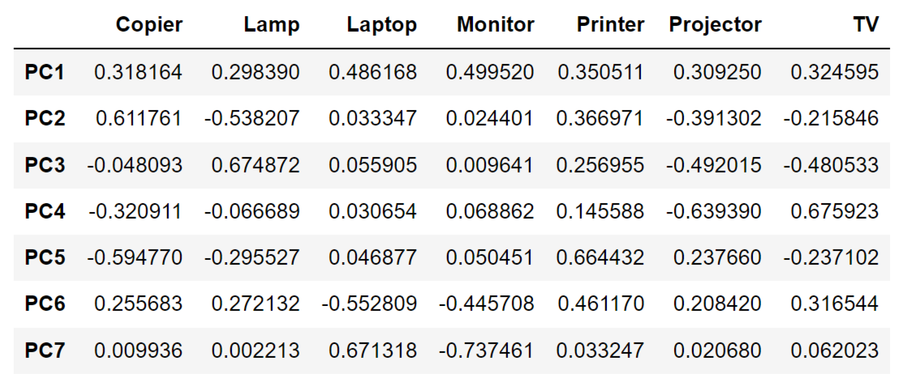
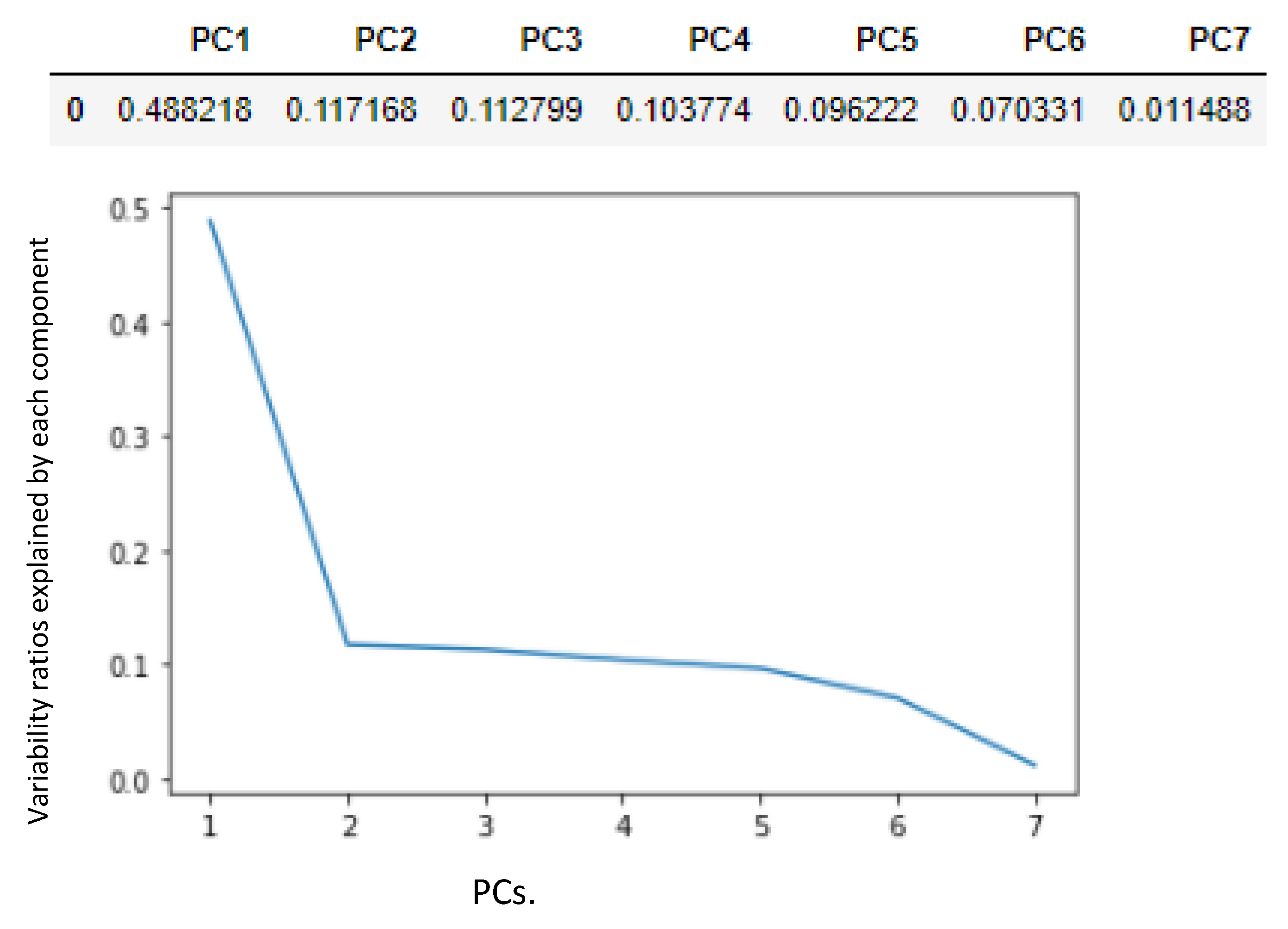
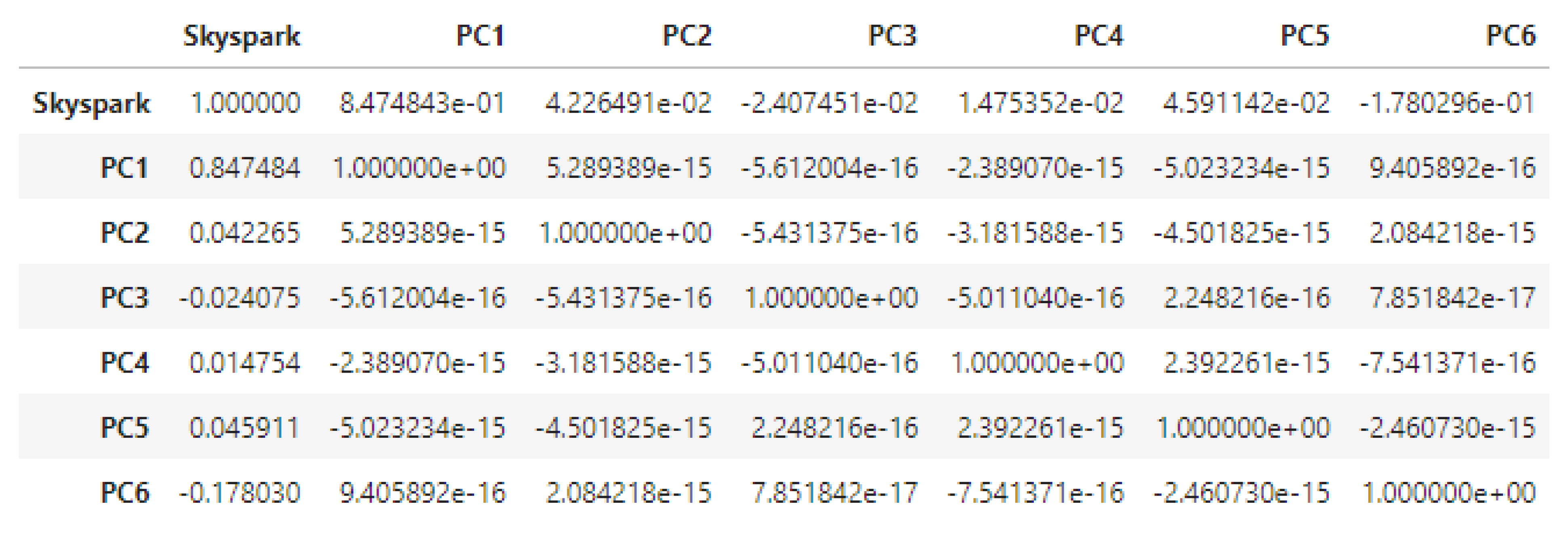
3.1.5. Principal Component Analysis (PCA)

This technique can reduce the dimensionality of the time-series, so that in each Principal Component (PC), we have a degree of information about each of the variables. Note that the PCs are not correlated between them. After normalizing the values of the dataset, PCA is applied to the selected descriptor variables (Copier, Lamp, Laptop, Monitor, Printer, Projector, and TV). Figure 7 shows the PCs calculated from these variables.

Figure 8 shows how much information about each variable is contained in each PC. In addition, the sign indicates whether the relationship between the component and the variable is direct or inverse.

For example, this means that PC1 is calculated as:

$$\begin{array}{c}PC1=0.318164\ast Copier+0.298390\ast Lamp+0.486168\ast Laptop+0.499520\ast Monitor+0.350511\\ \ast Printer+0.309250\ast Projector+0.324595\ast Tp\end{array}$$

The other components are calculated analogously.

On the other hand, the PCs are arranged in descending order according to their eigenvalues (that is, those that best explain the variability of the dataset are first). This is shown in

Table 2. Explained variability of each PC.

PC1	PC2	PC3	PC4	PC5	PC6	PC7
3.4175	0.8202	0.7896	0.7264	0.6735	0.4923	0.0804

, where it can be seen that PC1 has an explained variability of 3.417665, much higher than the following components.

However, to get a better idea of the proportion of explained variability of each component, the ratios of explained variability are analyzed. This is more intuitive information to select the PCs.

Table 3. Cumulative Explained Variability Ratios.

PC1	PC2	PC3	PC4	PC5	PC6	PC7
0.4882	0.6053	0.7181	0.8219	0.9181	0.9885	1.0

shows the accumulated explained variability ratios. One way to choose the components is to select those that reach a certain threshold. In this case, for a threshold of 98% of explained variability, the first 6 PCs can be selected, since they explain 98.85% of the variability.

Another option for selecting the number of PCs is to use the elbow method. In order to do this, the variability ratios explained by each component are graphically displayed, and the PC from which the curve flattens is identified, since the following components do not include relevant information on the initial variables. Figure 9 shows these ratios. It can be seen that the value drops considerably in PC2, confirming that PC1 explains much of the total variability.

Based on the above analysis, different numbers of PCs can be used. The former provides the greatest amount of information according to Table 3 and Figure 9, but up to PC6, there is an important accumulation of information. After this analysis, it is decided that the first six PCs be considered for further analysis.

Now, it is possible to determine the time window to generate the prediction models. In order to do this, the autocorrelations and the ARIMA models are used, both for the target variable and for each component.

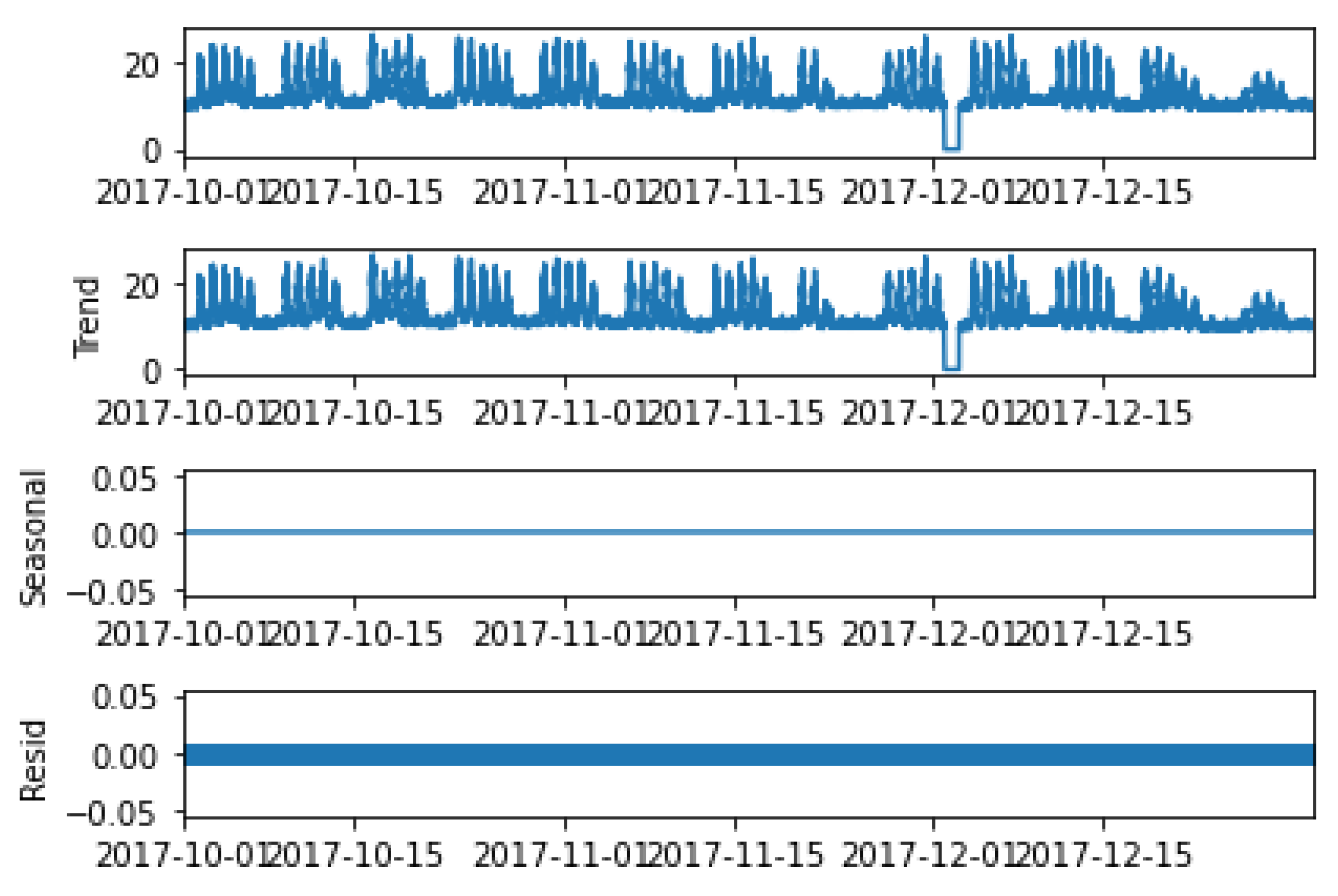
3.1.6. Analysis Using ARIMA Models

ARIMA models are an approach to time series forecasting which seeks to describe the autocorrelations in the data. The AR in ARIMA indicates an autoregression model, i.e., it forecasts the variable of interest using a linear combination of past (i.e., prior) values of the variable. The MA in ARIMA indicates a moving average model, i.e., it uses past forecast errors in a regression model (the regression error is a linear combination of errors in the past). Finally, the I in ARIMA indicates that the data values have been replaced with the differences between consecutive observations (the difference between their values and their previous values). Thus, an ARIMA model is defined as ARIMA (p,d,q), where p is the order of the autoregressive model, d is the degree of differencing involved, and q is the order of the moving average model:

$$y_t^{\prime }=c+{\alpha }_1{y}_{t-1}^{\prime }+\dots +{\alpha }_p{y}_{t-p}^{\prime }+{\epsilon }_{t-1}+{\beta }_1{\epsilon }_{t-1}+\dots +{\beta }_q{\epsilon }_{t-q}$$

where $y_t^{\prime }$ is the differenced series, c is a constant, ${\alpha }_i$ are the parameters of the autoregressive model, ${\beta }_i$ are the parameters of the moving average model, and ${\epsilon }_i$ are error terms. Thus, the purpose of an ARIMA model with these features is to make the model fit the data as well as possible.

In this section, the ARIMA models for each variable are generated automatically. Before applying this, it is guaranteed that each variable is non-stationary. In the previous section, this has been performed visually through the trend and seasonality figures, but to perform it systematically, we use the Dickey–Fuller test.

Starting with the target variable (Skyspark), the Dickey–Fuller test returns a p-value of 0.01. This value is below the threshold of statistical significance of 0.05, which indicates that the series is, in effect, non-stationary. Once the non-stationarity has been verified, the ARIMA model for Skyspark is obtained. The model obtained has a value of 5 as a parameter p and a value of 1 as a parameter q. Similarly, this process is repeated for the other PCs. However, it will not be applied to the six components selected, but only to those that are more correlated with Skyspark and have a high variability ratio/explained variability. These components are PC1 and PC2, as is shown in Figure 10 using the Pearson correlation, Table 2, and Figure 9.

The Dickey–Fuller test indicates that the time series in both components is stationary. After this, it is possible to obtain their respective ARIMA models. For PC1, the parameter p has a value of 5 and q of 0, while for PC2, the parameter p has a value of 5 and q has a value of 1.

Table 4. Parameters p and q of the ARIMA models.

Model	p	q
Skyspark	5	1
PC1	5	0
PC2	5	1

shows the p and q values of the adjusted models for each variable.

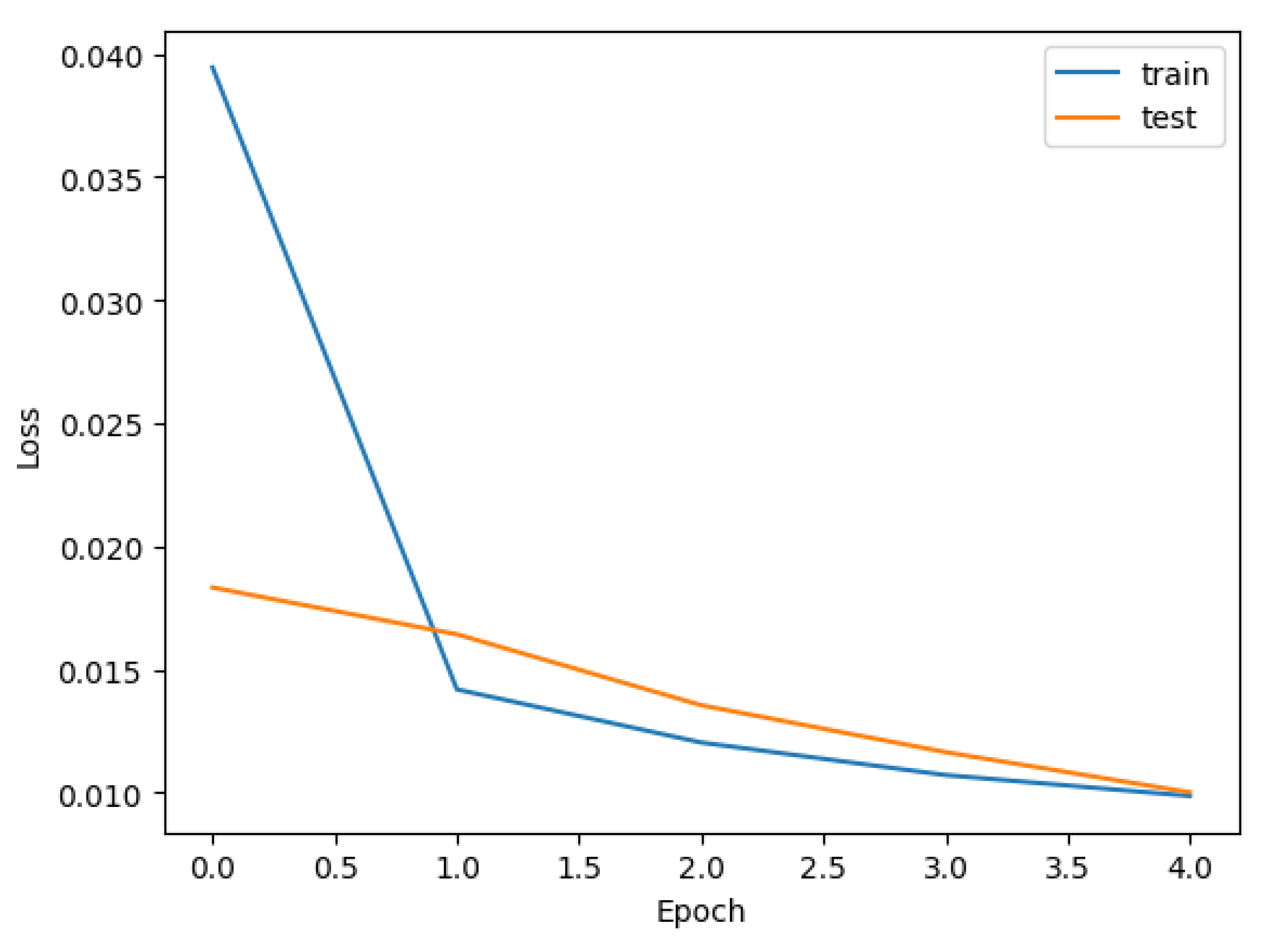
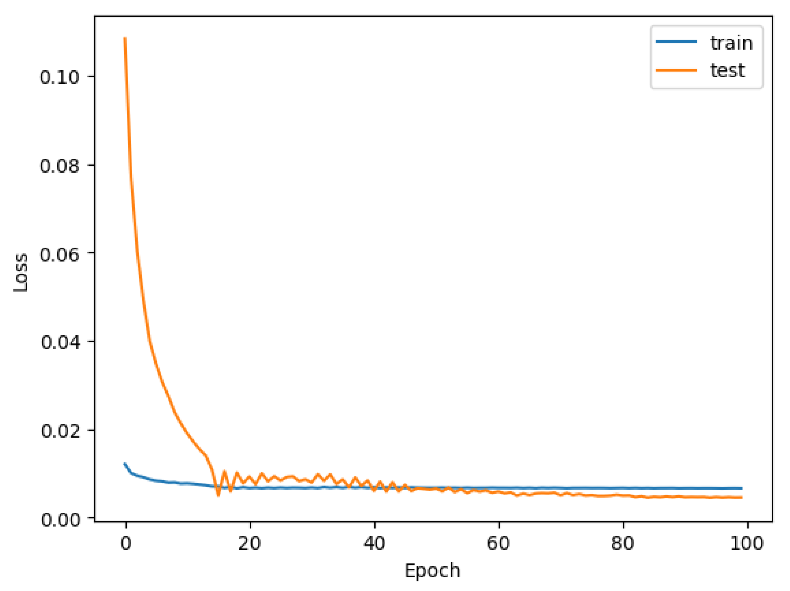
3.2. Generation and Evaluation of the Forecasting Models Using LSTM

For the modeling phase, it has been decided that LSTM neural networks would be used due to their advantages. In order to accomplish this, it is necessary to determine the time intervals to be used for the predictions. According to the feature engineering process results, it was decided that three groups of models be formed.

The first group consists of prediction models, in which only PC1 is used, since it is the variable most correlated with the target variable. The second group includes, in addition to PC1, PC2, because it is the second-most correlated variable with Skyspark. Finally, in the third group, the Skyspark estimation is carried out from the original variables after the feature engineering process, in order to determine if the extraction/fusion of characteristics has provided any advantage.

Given that, for the three variables, a value of 5 was obtained as the parameter p of the ARIMA models, this being greater than the value of the parameter q in the three cases, the three groups of models were tested with lags of t−5. The modeling process follows the following steps:

First, the values are normalized and the predictor variables are separated from the target variable. LSTM neural networks require that the input dataset be a three-dimensional array: number of observations, number of time intervals, and number of variables. In this way, for each observation, there is an array for each time interval to take into account, including the current instant and the established delays.

Once the dataset has been prepared according to the time window, it is necessary to divide the total observations into training data (70%) and test data (30%).

The predictive models are generated with the training data. The number of neurons and epochs are adjusted according to the results. As the loss function, the Least Squared Errors metric is used.

The quality of each model is determined using RMSE, MAPE, and R² metrics.

Before creating the three groups of models, it is decided that an initial prediction model be generated using the variables selected by the feature engineering process before reaching the dimension analysis process, which will serve as a starting point to adjust both the number of neurons and epochs in the following groups of models. In order to produce this first model, the established time window is related to the number of neurons and training epochs of the LSTM network. Therefore, the model is generated with a network composed of five neurons in the hidden layer and trained in five epochs. Figure 11 shows the loss function for the training and test datasets. It can be seen that the values for the test dataset do not reach the values of the training dataset, remaining higher at all points.

On the other hand, the prediction quality metrics are not optimal enough. Regarding the errors obtained, RMSE is 0.10, MAPE is 0.17, and R² is 0.40. Given these inaccurate results, it was decided that a greater number of neurons and training periods be tested in each of the groups, with the aim of obtaining better prediction models.

3.2.1. Group 1: PC1 and Skyspark

After a process of hyperparameterization of the LSTM for the number of neurons and training epochs, the best model was with 100 neurons and 100 training epochs. Figure 12 shows that the loss function for the test data reaches the loss values of the training data before epoch 20. Thereafter, it undergoes small fluctuations, but these fluctuations gradually disappear. The quality metrics are: RMSE is 0.07, MAPE is 0.10, and R² is 0.74.

3.2.2. Model Group 2: PC1, PC2 and Skyspark

In a similar way to the first group, after an hyperparameterization process for the number of neurons and training periods, the best model was for 50 neurons and 100 training epochs. In this case, the loss function of the test data set reaches the values of the training data set shortly after epoch 20, as seen in Figure 13. Although small variations occur from that point, the function tends eventually to stabilize. Regarding the quality metrics, RMSE is 0.07, MAPE is 0.11, and R² is 0.72.

3.2.3. Model Group 3: Original Variables and Skyspark

Unlike the previous groups, these models are not generated with the PCs as input data. Instead, the input data set for the models in this group corresponds to the original variables before applying PCA, determined by our feature engineering process.

In this case, after the hyperparameterization process, the best LSTM model was with 50 neurons and 100 epochs. In this case, the loss function for the test data set appears stable, descending until reaching the loss values of the training data set around epoch 20 (see Figure 14). Regarding the prediction quality metrics, RMSE is 0.07, MAPE is 0.12, and R² is 0.74.

3.3. Comparison of the Forecasting Models of Each Group

According to [21,22], the relevant LSTM hyperparameters to be optimized are the number of neurons and epochs (number of times each training example is passed through the network). In the previous subsections, we have optimized them for each different set of input data. In this section, we compare the best LSTMs obtained for each input dataset.

Comparing the results of the groups, we can see they are very similar. In some cases, the errors or precision are better or worse. In addition, the optimal number of neurons and training epochs is very variable in each group. Starting from the best models obtained in each group, summarized in

Table 5. Summary of best models of each group.

Group	No. of Neurons	No. of Epochs	RMSE	MAPE	R2
1	100	100	0.07	0.10	0.74
2	50	100	0.07	0.11	0.72
3	50	100	0.07	0.12	0.74

, we make a comparison between them. In the first group, better results were obtained with a model of 100 neurons and 100 training periods, while in the second group, the best results were obtained with a model of 50 neurons and 100 training periods.

According to the results, the inclusion of PC2 as a descriptive variable does not provide advantages to the generation of an optimal model. It can even be said that it negatively affects the learning process, since it causes the neural network to take into account a greater amount of input data, which does not provide relevant information, since PC2 does not have a significant correlation with the target variable (Skyspark). Therefore, from this first comparison, the model from the first group can be selected as the best option.

On the other hand, in the third group are obtained predictions as accurate as those of the first group. In particular, in the third group, the variables used are the ones selected by the initial feature engineering process, before reaching the dimensional analysis phase, which is where PCA is used (see Figure 2). Specifically, the results indicate that the phase of analysis of the correlations to determine the descriptive variables to use (the first phase of our feature engineering process, see Figure 2) is quite good, since similar results are obtained when using PC1. These variables are sufficiently correlated with Skyspark to provide relevant information in the learning process. In addition, including a greater number of variables requires more neurons and training cycles to achieve a model with a performance similar to the first group. However, increasing the number of neurons and epochs can lead to overfitting, causing less accurate predictions. This is reflected in the cases in which the loss function for the test data set presents values below those of the loss function for the training data set (see Figure 14) [33].

Thus, this third group model seems a viable option. However, if we review the loss function for this model, we see that it undergoes variations for the test data set, which means that it is not truly a stable model. That is, in certain cases, it can give good predictions, and in other cases, it cannot. From this, we can say that, although considering the initial variables as descriptors can give good results, it does not assure us that this happens in all cases. Once the best models of each group have been compared, the model of the first group is the most appropriate.

In general, in the case of very few epochs, the network does not learn enough, producing underfitting, as in the case of the initial model of 5 neurons and 5 training epochs, where the values of the loss function for the test data set are very low [33]. On the contrary, if there are many epochs, the model begins to memorize and stops learning, producing overfitting, as observed in the cases in which the loss function for the test data set goes below that of the training data set [33].

Finally, some possible extensions to this study concern the use of other concepts in the feature engineering process [32,34,35], such as the evaluation of the temporal dependence relationship of the descriptor variables using regressors combined with the autoregression of the objective variable [34,35], the use of a descriptor variable selection algorithm that uses different criteria in real-time for said selection [36,37], and their effects on the behavior of predictive models. In addition, the use of techniques that allow the construction of explanatory predictive models for time series is important in the energy field, such as cognitive maps [38,39], and will require analysis of variables and parameters similar to the one proposed in this work.

4. Comparison of LSTM with Other Techniques

In order to show the feasibility of the feature engineering process proposed in this work, several datasets are used in this section. Specifically, for each dataset, a feature engineering process is carried out according to the steps shown in Section 3, which:

−

Studies the temporal relationship between the variable to be predicted and the rest of the variables;

−

Performs a feature reduction analysis using PCA.

With the results of the feature engineering process, prediction models are built using LSTM and other techniques in order to compare them (see

Table 6. Results of the predictive models in different datasets and techniques.

Dataset	Technique	RMSE	MAPE	R2
[40]	Gradient boosting	0.0249	75.7002	0.9937
	Random forest	0.0244	75.4282	0.9928
	LSTM	0.0101	75.3260	0.9920
	L-BFGS	0.0220	76.7360	0.9939
	CNN	0.0229	75.7002	0.9936
[41]	Gradient boosting	0.0331	21.6070	0.9750
	Random forest	0.0351	21.5721	0.9600
	LSTM	0.0310	19.4190	0.9710
	L-BFGS	0.0320	19.4860	0.9570
	CNN	0.0663	21.6816	0.9019
[42]	Gradient boosting	0.0395	17.1182	0.9309
	Random forest	0.0457	17.4153	0.9336
	LSTM	0.0417	15.0250	0.9497
	L-BFGS	0.0487	15.1240	0.9393
	CNN	0.0608	17.0162	0.9401
[43]	Gradient boosting	0.0645	17.5819	0.9352
	Random forest	0.0914	18.0262	0.8930
	LSTM	0.0625	17.3260	0.9147
	L-BFGS	0.0910	22.7140	0.9126
	CNN	0.1318	19.8812	0.8966
[44]	Gradient boosting	0.1415	21.7193	0.6254
	Random forest	0.1177	21.9066	0.6694
	LSTM	0.1351	21.0200	0.7300
	L-BFGS	0.1313	21.0180	0.7430
	CNN	0.0973	21.0040	0.7671

). For each model used, as for the LSTM model, an hyperparameter optimization process is performed. For example, for the LSTM model and dataset [40], the best results were with 30 neurons and 25 epochs; for dataset [41], 40 neurons and 40 epochs; for dataset [42], 120 neurons and 60 epochs; and for dataset [43], 100 neurons and 40 epochs.

According to the results, we see that our approach to pre-toning the LSTM with our feature engineering process to define the backward sequence of the technique makes it a very robust method. In particular, in the different datasets, it obtains the best result (see colors in bold), or it is always among the best. Of the other techniques evaluated, some of their metrics are never among the best (for example, random forest), or they are good in some cases and not in others (for example, CNN).

Thus, we can see that our feature engineering process to establish the temporal relationships of the time series that describe energy consumption is necessary. In addition, this indicates the need for such a process, and for techniques such as LSTM, in energy consumption prediction tasks. Particularly, this process gives a lot of robustness to the LSTM technique, regardless of the energy consumption dataset (time series).

5. Conclusions

This research presents an analysis of the energy consumption forecasting problem. The paper carries out an analysis proposing a feature engineering process to obtain the variables to be used in the predictive models. The results of this process are used to build different energy consumption prediction models using the LSTM technique. In this context, different groups are defined in order to build the predictive models and to experiment with them.

The main contribution is the feature engineering methodological approach created to analyze the energy consumption variables of buildings. This approach defines several phases to study the time series that define energy consumption in buildings. Particularly, it proposes an analysis phase of the dependency relations between the variables (correlations), as well as the temporal ones (regressors). In addition, it proposes an analysis phase of the dimensions in the dataset to fuse/extract characteristics. Thus, in the feature engineering process, thanks to the correlation coefficients and linear regression models, we analyze the relationships between the variables, and with these results, we perform the feature extraction/fusion by applying PCA. Another aspect to be considered is the temporal relationship of the variables with themselves. For this, we rely on the models of autocorrelation and ARIMA, thanks to which we obtain the optimal time window to make the predictions.

Finally, we have compared LSTM with other machine learning techniques, using our feature engineering process to analyze the time series of various energy consumption datasets (temporal series). Based on the results, we see that this feature engineering process helps LSTM to obtain an excellent fit of the time sequences to be considered, in order to build a predictive model. This quality is the best in the group of datasets tested, since their metrics are the best, or are consistently among the best.

The next steps in our work are: (i) to analyze the impact of other feature engineering processes that can be used with time series; (ii) to define an adaptation mechanism of the predictive model in real-time; (iii) to analyze the effect of inclusion of new variables like climatological variables in our dataset. Climatic factors affect energy consumption since, depending on these values, devices such as heating or air conditioning are used to a greater or lesser extent. In addition, these variables have a marked temporality.

References

1. Aguilar, J.; Garces-Jimenez, A.; R-Moreno, M.D.; García, R. A systematic literature review on the use of artificial intelligence in energy self-management in smart buildings. Renew. Sustain. Energy Rev. 2021, 151, 111530. [Google Scholar] [CrossRef]
2. Minoli, D.; Sohraby, K.; Occhiogrosso, B. IoT considerations, requirements, and architectures for smart buildings—Energy optimization and next-generation building management systems. IEEE Internet Things J. 2017, 4, 269–283. [Google Scholar] [CrossRef]
3. Rodriguez-Mier, P.; Mucientes, M.; Bugarín, A. Feature Selection and Evolutionary Rule Learning for Big Data in Smart Building Energy Management. Cogn. Comput. 2019, 11, 418–433. [Google Scholar] [CrossRef]
4. García, D.; Goméz, M.; Noguera, F.V. A Comparative Study of Time Series Forecasting Methods for Short Term Electric Energy Consumption Prediction in Smart Buildings. Energies 2019, 12, 1934. [Google Scholar]
5. Alduailij, M.; Petri, I.; Rana, O.; Alduailij, M.; Aldawood, A. Forecasting peak energy demand for smart buildings. J. Supercomput. 2021, 77, 6356–6380. [Google Scholar] [CrossRef]
6. Hernández, M.; Hernández-Callejo, L.; Solís, M.; Zorita-Lamadrid, A.; Duque-Perez, O.; Gonzalez-Morales, L.; Santos-García, F. Data-Driven Forecasting Strategy to Predict Continuous Hourly Energy Demand in Smart Buildings. Appl. Sci. 2021, 11, 7886. [Google Scholar] [CrossRef]
7. Hernández, M.; Hernández-Callejo, L.; García, F.; Duque-Perez, O.; Zorita-Lamadrid, A. A Review of Energy Consumption Forecasting in Smart Buildings: Methods, Input Variables, Forecasting Horizon and Metrics. Appl. Sci. 2020, 10, 8323. [Google Scholar] [CrossRef]
8. Moreno, M.; Dufour, L.; Skarmeta, A. Big data: The key to energy efficiency in smart buildings. Soft Comput. 2016, 20, 1749–1762. [Google Scholar] [CrossRef] [Green Version]
9. Nabavi, S.; Motlagh, N.; Zaidan, M.; Aslani, A.; Zakeri, B. Deep Learning in Energy Modeling: Application in Smart Buildings with Distributed Energy Generation. IEEE Access 2021, 9, 125439–125461. [Google Scholar] [CrossRef]
10. Somu, N.; Raman, G.; Ramamritham, K. A hybrid model for building energy consumption forecasting using long short term memory networks. Appl. Energy 2020, 261, 114131. [Google Scholar] [CrossRef]
11. Le, T.; Vo, M.; Kieu, T.; Hwang, E.; Rho, S.; Baik, W. Multiple Electric Energy Consumption Forecasting Using a Cluster-Based Strategy for Transfer Learning in Smart Building. Sensors 2020, 20, 2668. [Google Scholar] [CrossRef] [PubMed]
12. Hadri, S.; Naitmalek, Y.; Najib, M.; Bakhouya, M.; Fakhri, Y.; Elaroussi, M. A Comparative Study of Predictive Approaches for Load Forecasting in Smart Buildings. Procedia Comput. Sci. 2019, 160, 173–180. [Google Scholar] [CrossRef]
13. González-Vidal, A.; Jiménez, F.; Gómez-Skarmeta, A.F. A methodology for energy multivariate time series forecasting in smart buildings based on feature selection. Energy Build. 2019, 196, 71–82. [Google Scholar] [CrossRef]
14. González-Vidal, A.; Ramallo-González, A.; Terroso-Sáenz, F.; Skarmeta, A. Data driven modeling for energy consumption prediction in smart buildings. In Proceedings of the IEEE International Conference on Big Data, Boston, MA, USA, 11–14 December 2017; pp. 4562–4569. [Google Scholar]
15. Sülo, S.; Keskin, G.; Dogan, T.; Brown, T. Energy Efficient Smart Buildings: LSTM Neural Networks for Time Series Prediction. In Proceedings of the International Conference on Deep Learning and Machine Learning in Emerging Applications, Istanbul, Turkey, 26–28 August 2019; pp. 18–22. [Google Scholar]
16. Aliberti, A.; Bottaccioli, L.; Macii, E.; di Cataldo, S.; Acquaviva, A.; Patti, E. A Non-Linear Autoregressive Model for Indoor Air-Temperature Predictions in Smart Buildings. Electronics 2019, 8, 979. [Google Scholar] [CrossRef] [Green Version]
17. Alawadi, S.; Mera, D.; Fernández-Delgado, M. A comparison of Machine Learning algorithms for forecasting indoor temperature in smart buildings. Energy Syst. 2020, 13, 689–705. [Google Scholar] [CrossRef] [Green Version]
18. Siddiqui, A.; Sibal, A. Energy Disaggregation in Smart Home Appliances: A Deep Learning Approach. Energy, 2021; in press. [Google Scholar]
19. Bhatt, D.; Hariharasudan, A.; Lis, M.; Grabowska, M. Forecasting of Energy Demands for Smart Home Applications. Energies 2021, 14, 1045. [Google Scholar] [CrossRef]
20. Escobar, L.M.; Aguilar, J.; Garcés-Jiménez, A.; de Mesa, J.A.G.; Gomez-Pulido, J.M. Advanced Fuzzy-Logic-Based Context-Driven Control for HVAC Management Systems in Buildings. IEEE Access 2020, 8, 16111–16126. [Google Scholar] [CrossRef]
21. Bourhnane, S.; Abid, M.; Lghoul, R.; Zine-Dine, K.; Elkamoun, N.; Benhaddou, D. Machine Learning for energy consumption prediction and scheduling in smart buildings. SN Appl. Sci. 2020, 2, 297. [Google Scholar] [CrossRef] [Green Version]
22. Hadri, S.; Najib, M.; Bakhouya, M.; Fakhri, Y.; el Arroussi, M. Performance Evaluation of Forecasting Strategies for Electricity Consumption in Buildings. Energies 2021, 14, 5831. [Google Scholar] [CrossRef]
23. Khan, A.-N.; Iqbal, N.; Rizwan, A.; Ahmad, R.; Kim, D. An Ensemble Energy Consumption Forecasting Model Based on Spatial-Temporal Clustering Analysis in Residential Buildings. Energies 2021, 14, 3020. [Google Scholar] [CrossRef]
24. Keytingan, M.; Shapi, M.; Ramli, N.; Awalin, L. Energy consumption prediction by using machine learning for smart building: Case study in Malaysia. Dev. Built Environ. 2021, 5, 100037. [Google Scholar]
25. Son, N.; Yang, S.; Na, J. Deep Neural Network and Long Short-Term Memory for Electric Power Load Forecasting. Appl. Sci. 2020, 10, 6489. [Google Scholar] [CrossRef]
26. Moon, J.; Park, S.; Rho, S.; Hwang, E. Robust building energy consumption forecasting using an online learning approach with R ranger. J. Build. Eng. 2022, 47, 103851. [Google Scholar] [CrossRef]
27. Pinto, T.; Praça, I.; Vale, Z.; Silva, J. Ensemble learning for electricity consumption forecasting in office buildings. Neurocomputing 2021, 423, 747–755. [Google Scholar] [CrossRef]
28. Somu, N.; Raman, G.; Ramamritham, K. A deep learning framework for building energy consumption forecast. Renew. Sustain. Energy Rev. 2021, 137, 110591. [Google Scholar] [CrossRef]
29. Amidi, S. Recurrent Neural Networks Cheatsheet. Available online: https://stanford.edu/~shervine/teaching/cs-230/cheatsheet-recurrent-neural-networks (accessed on 15 April 2021).
30. Yuan, X.; Li, L.; Wang, Y. Nonlinear Dynamic Soft Sensor Modeling with Supervised Long Short-Term Memory Network. IEEE Trans. Ind. Inform. 2021, 16, 3168–3176. [Google Scholar]
31. Doherty, K. Trenbath, Raw_Data, CO, USA: Mendeley Data. 2019. Available online: https://data.mendeley.com/datasets/g392vt7db9/1 (accessed on 15 April 2021).
32. Aguilar, J.; Terán, O. Modelo del proceso de Influencia de los Medios de Comunicación Social en la Opinión Pública. Educere 2018, 22, 179–191. [Google Scholar]
33. Brownlee, J. Multivariate Time Series Forecasting with LSTMs in Keras. Available online: https://machinelearningmastery.com/multivariate-time-series-forecasting-lstms-keras/ (accessed on 15 April 2021).
34. Quintero, Y.; Ardila, D.; Camargo, E.; Rivas, F.; Aguilar, J. Machine learning models for the prediction of the SEIRD variables for the COVID-19 pandemic based on a deep dependence analysis of variables. Comput. Biol. Med. 2021, 134, 104500. [Google Scholar] [CrossRef]
35. Cavaleiro, J.; Neves, M.; Hewlins, M.; Jackson, A. The photo-oxidation of meso-tetraphenylporphyrins. J. Chem. Soc. 1990, 7, 1937–1943, Perkin Transactions 1. [Google Scholar] [CrossRef]
36. Jiménez, M.; Aguilar, J.; Monsalve-Pulido, J.; Montoya, E. An automatic approach of audio feature engineering for the extraction, analysis and selection of descriptors. Int. J. Multimed. Info. Retr. 2021, 10, 33–42. [Google Scholar] [CrossRef]
37. Aguilar, J.; Salazar, C.; Velasco, H.; Monsalve-Pulido, J.; Montoya, E. Comparison and Evaluation of Different Methods for the Feature Extraction from Educational Contents. Computation 2020, 8, 30. [Google Scholar] [CrossRef]
38. Aguilar, J. A Fuzzy Cognitive Map Based on the Random Neural Model. Lect. Notes Comput. Sci. 2001, 2070, 333–338. [Google Scholar]
39. Sánchez, H.; Aguilar, J.; Terán, O.; de Mesa, J.G. Modeling the process of shaping the public opinion through Multilevel Fuzzy Cognitive Maps. Appl. Soft Comput. 2019, 85, 105756. [Google Scholar] [CrossRef]
40. Papaioannou, T.; Stamoulis, G. Teaming and competition for demand-side management in office buildings. In Proceedings of the IEEE International Conference on Smart Grid Communications (SmartGridComm), Dresden, Germany, 23–26 October 2017; pp. 332–337. [Google Scholar]
41. Power Consumption Data of a Hotel Building. Available online: https://ieee-dataport.org/documents/power-consumption-data-hotel-building (accessed on 15 April 2021).
42. Zhang, L.; Wen, J. A systematic feature selection procedure for short-term data-driven building energy forecasting model development. Energy Build. 2019, 183, 428–442. [Google Scholar] [CrossRef]
43. Pipattanasomporn, M.; Chitalia, G.; Songsiri, J.; Aswakul, C.; Pora, W.; Suwankawin, S.; Audomvongseree, K.; Hoonchareon, N. CU-BEMS, smart building electricity consumption and indoor environmental sensor datasets. Sci. Data 2020, 7, 241. [Google Scholar] [CrossRef]
44. Long-Term Energy. Consumption & Outdoor Air Temperature for 11 Commercial Buildings. Available online: https://trynthink.github.io/buildingsdatasets/show.html?title_id=long-term-energy-consumption-outdoor-air-temperature-for-11-commercial-buildings (accessed on 15 April 2021).
Figure 1. Architecture of a neuron in an LSTM network.
Sustainability 14 13358 g001
Figure 2. Feature Engineering Process for Energy Datasets of Smart Buildings.
Sustainability 14 13358 g002
Figure 3. Pearson’s correlation coefficient matrix.
Sustainability 14 13358 g003
Figure 4. Spearman’s correlation coefficient matrix.
Sustainability 14 13358 g004
Figure 5. Autocorrelation of Skyspark. (a) Simple Skyspark autocorrelation. (b) Partial autocorrelation of Skyspark.
Sustainability 14 13358 g005
Figure 6. Decomposition of the time series of the Skyspark variable.
Sustainability 14 13358 g006
Figure 7. PCs for our case study.
Sustainability 14 13358 g007
Figure 8. Relationship between PCs and variables.
Sustainability 14 13358 g008
Figure 9. Explained variability ratios by each PC.
Sustainability 14 13358 g009
Figure 10. Pearson’s Correlation of the PCs.
Sustainability 14 13358 g010
Figure 11. The loss function for 5 neuron models and 5 training epochs.
Sustainability 14 13358 g011
Figure 12. Best results of the loss functions for Group 1.
Sustainability 14 13358 g012
Figure 13. Best results of the loss functions for Group 2.
Sustainability 14 13358 g013
Figure 14. Loss functions for Group 3.
Sustainability 14 13358 g014