Charging Strategies for Battery Electric Trucks in Germany

Abstract

Battery electric trucks (BETs) are a promising option to reduce emissions from heavy-duty vehicles. However, the transition to BETs will cause an additional demand for electricity. Future charging strategies will influence the future peak load as well as the operational and technical feasibility of BETs. We simulated 2410 representative single-day German truck driving profiles with three different charging strategies: (1) as slow as possible, (2) as fast as possible, and (3) slowly at depots and as fast as possible at public locations. Assuming a 33% electrification rate by 2030 and near-complete fleet conversion by 2045, we scaled our results to the German truck fleet. We found that charging as fast as possible leads to additional peak loads up to 6 GW in 2030 and 18 GW in 2045, while the other charging strategies reduce additional peak loads to 3 GW in 2030 and 8 GW in 2045. Therefore, implementing wise charging strategies will reduce future peak load.

1. Introduction

Heavy-duty vehicles (HDVs) account for 5% of the European vehicle fleet but caused approximately one-quarter of greenhouse gas emissions in the transport sector in 2023 [1]. Climate neutrality necessitates ambitious measures in the transport sector, with electrification as the most likely option for HDVs [2,3]. The first battery electric trucks (BETs) are already available, and European manufacturers anticipate about half of all trucks sold by 2030 to be BETs [3]. Megawatt charging will enable trucks to charge within the legally binding 45 min driver break. By 2045, approximately 45 TWh—a quarter of the expected electricity demand in the transport sector in Germany—could be needed for HDVs [4].

Earlier publications have focused on the economic feasibility of BETs [5,6,7,8], their technical feasibility [9,10,11], and the regional demand for charging infrastructure [12,13,14,15]. The European Commission aims to provide charging stations for BETs at a maximum distance of 60 km along the main traffic routes (TEN-T Core network) and at a maximum distance of 100 km along the TEN-T Comprehensive network by the end of 2030 [16]. In total, studies indicate that the majority of logistics operations can be electrified. The higher the annual mileage, the greater the economic benefits of BETs compared to diesel vehicles. Simultaneously, technical feasibility decreases at higher mileage, making public charging infrastructure necessary.

Assuming optimal charging strategies, analyses show that charging can be integrated into the daily logistics processes. For a large share of the fleet, depot charging is the most relevant option to recharge. Public megawatt charging as an intermediate charging option is relevant for vehicles with a high daily mileage [17,18].

However, different charging strategies influence the technical feasibility of BETs, as well as the associated load curve, and thus need to be evaluated. Based on a hypothetical fleet of 100 vehicles in California, illustrative analyses show that managed charging can avoid charging peaks and lower costs for logistics companies [19]. An exemplary study in the U.S. shows that depot charging can be integrated into existing electricity grids. The effect on the additional load is dependent on the applied charging strategy [20]. Similar to the results for the U.S., depot charging below 44 kW per truck enables the electrification of approximately 80% of the German truck fleet [18].

However, we are not aware of any studies examining the effects of different truck charging strategies at depots and public charging locations on a country’s temporally resolved energy demand. Therefore, this analysis aims to provide representative load profiles for a future German BET fleet in 2030 and 2045 under three different charging strategies. The charging strategies are differentiated by charging power, charging duration, and the location of the charging points. The analysis focuses on the expected additional peak load caused by BETs and the expected load curve on a country level.

This article is a revised and expanded version of a conference paper, which was presented at the 38th International Electric Vehicle Symposium in Gothenburg [21].

2. Materials

In the following, we briefly describe the underlying scenarios (Section 2.1) and the data used in the analyses (Section 2.2).

2.1. Scenario Descriptions

The scenario descriptions contain information on the charging behavior (Section 2.1.1) and on the expected BET fleet development in Germany (Section 2.1.2).

2.1.1. Charging Behavior

Our model distinguishes between private and public charging locations. Private charging locations are located on the premises of forwarding agencies or customers and on other private properties. Public charging locations include highway service stations and other public parking locations for trucks. However, while the dataset allows for this distinction, it does not provide georeferenced information. Therefore, a more detailed description of potential charging locations and the resulting overload of specific regional network nodes is not possible.

We distinguish three charging power categories. The first category covers charging power up to 44 kW, which is the maximum achievable using an alternating current (AC) plug. We refer to this category as “slow charging”. The second category covers a charging power of up to 350 kW, currently known in the passenger car sector as “Combined Charging System” (CCS). As a third category, the newly developed “Megawatt Charging System” (MCS) provides a charging power significantly higher than 350 kW [22]. Approximately 1 MW will be a suitable level for BETs [18]. For the sake of simplicity, we use “MCS charging” as nameplate for an average charging power between 350 kW and 1 MW, although charging with lower power could technically also be realized with MCS. It should be noted that we do not distinguish between charging power of up to 350 kW (referred to as “CCS charging”) and those more than 350 kW (referred to as “MCS charging”) in terms of modeling but evaluate them separately.

This analysis aims to provide representative load profiles for a future German BET fleet in 2030 and 2045, given three different charging strategies: (1) As slow as possible (ASAP). The entire time available for the charging process is used to charge the vehicle battery. The strategy aims to minimize the additional load on the electricity grid. (2) As fast as possible (AFAP). The charging process starts immediately after a trip is completed and ends when the battery is fully charged. This is the most challenging strategy for the electricity grid. (3) Combination. Private charging at the depot is limited to 44 kW and follows the ASAP strategy. Public charging follows the AFAP strategy. This strategy provides a real-world-oriented approach. In each strategy, the aim is to fully recharge the vehicle within the boundary conditions, if possible.

Table 1. Overview of charging strategies and their characteristics.

		ASAP	AFAP	Combination
Available charging power per vehicle	Private	≤44 kW ≤350 kW >350 kW	>350 kW	≤44 kW
	Public	≤44 kW ≤350 kW >350 kW	>350 kW	>350 kW
Charging strategy	Private	As slow as possible	As fast as possible	As slow as possible
	Public	As slow as possible	As fast as possible	As fast as possible

sums up the most important aspects.

The model only schedules a charging event if there is a minimum charging duration of 30 min available. This minimum charging period reflects the additional effort that comes with each additional charging event. In addition, the vehicle is only charged if the current battery level is not sufficient to cope with the next trip (c.f. Section 3) or if the previous trip was the last trip of the day. We assume that each vehicle starts the first trip of the day fully charged. As a simplification, we assume a continuous charging process at constant power, regardless of the current state of charge (SOC). Additionally, we apply no competition for charging points and therefore no waiting times.

2.1.2. Fleet Development

For simplification, we assume a constant HDV stock of 470,000 vehicles, even though one might argue that the stock will grow further in the future. A larger vehicle stock will potentially linearly increase the energy demand. By 2030, we assume that 33% of the German HDV fleet will be electrified [3,4]. By 2045, all vehicles that are technically eligible for electrification will be included, meaning that only those with driving profiles feasible for BET models will be transitioned accordingly. Driving profiles that are not feasible for BETs under the assumed parameters will continue to be served by conventional HDVs. Whether this transition is feasible depends on the charging strategy applied.

2.2. Data

The following sections provide information on the underlying driving data (Section 2.2.1) and technical assumptions (Section 2.2.2).

2.2.1. Driving Data

To model charging and driving behavior of BETs, we use real driving data from diesel vehicles, specifically the “Motor Vehicle Traffic in Germany 2010” (KiD) survey [23]. The analyzed vehicles were randomly selected from the central vehicle register of the Federal Motor Transport Authority (Kraftfahrt-Bundesamt) between October 2009 and November 2010 and the data were collected using questionnaires. The dataset contains 2810 single-day driving profiles from rigid trucks and tractor-trailers (>12 t GVW), representative for Germany. A total of 400 of these are excluded from the analyses in this paper, because they contain incomplete information on individual trips. We therefore use 2410 driving profiles for our analysis, consisting of 1350 rigid trucks and 1060 tractor-trailers profiles.

The KiD data include all trips of the sampled vehicles over a single day. The dataset contains, among other details, the following information for each vehicle: vehicle ID, size (“rigid” or “tractor-trailer”), gross vehicle weight (in kg), daily mileage (in km), the number of trips, and information on individual trips. A single trip includes the departure and the arriving time, the distance traveled during the trip (in km), and the type of parking location. We define company premises, private properties, and parking lots as private. Public parking spaces as well as unknown locations are defined as public. Unfortunately, the dataset does not include geographical information on specific locations, meaning that the type of origin and destination parking locations and the traveled distance are known, but not the actual coordinates. Figure 1 illustrates the distribution of the daily mileage in the sample. It is evident that driving profiles for all types of use are included in the calculations. We consider trucks used for long-, medium- and short-distance transportation.

2.2.2. Technical Assumptions

We define the minimum range that a fully charged BET can travel without scheduling an additional charging event. The minimum range is defined as 80% of the maximum range [18]. In 2030, a minimum range of 280 km is assumed. In 2045, we assume 470 km. Therefore, the maximum achievable distance for BETs in 2030 is assumed to be 350 km and 590 km in 2045. Please note that the maximum range does not refer to the highest range available for a newly registered vehicle, but rather to the average range for a stock vehicle in the corresponding year, based on announcements from truck manufacturers [24,25]. Furthermore, the range in 2030 covers the legally binding maximum driving time of 4.5 h [26].

We estimate the maximum average charging capacities to be 430 kW in 2030 and 810 kW in 2045 (own assumptions, based on [3]). Maximum average charging capacity means the highest possible average charging power during a whole charging event. Peak power may be higher. Moreover, we estimate an energy consumption of 1.12 kWh/km for rigids and 1.24 kWh/km for tractor-trailers in 2030. These will improve in 2045 to 0.95 kWh/km for rigids and 1.06 kWh/km for tractor-trailers [18]. For simplicity, we assume constant energy consumption, though practical implementation must consider factors such as weather conditions, driving behavior, road topography, loading and design. As these conditions may influence the energy demand [27], we added a sensitivity analysis and the Monte Carlo simulation in Section 4.4.

Table 2. Assumed technical vehicle data for 2030 and 2045.

	Minimum Range [km]	Maximum Range [km]	Maximum Charging Power [kW]	Energy Consumption of Rigid Truck [kWh/km]	Energy Consumption of Tractor-Trailer Truck [kWh/km]
2030	280	350	430	1.12	1.24
2045	470	590	810	0.95	1.06

summarizes the most important technical vehicle assumptions.

3. Methods

The goal of the model is to determine the charging and driving patterns of the individual vehicles at five-minute intervals throughout the day (1440 min). We use an agent-based simulation to model each driving profile separately, providing a highly realistic representation of fleet electrification.

In the first step, the driving and parking behavior of each vehicle is simulated. Departure and arrival timestamps for each trip and vehicle are converted into a discrete-time simulation. Using the start and arrival times, along with the distance traveled data from the KiD dataset for each vehicle and trip, the vehicle’s status (private parking, public parking, or driving) and the distance traveled at specific timestamps are recorded in five-minute intervals.

Truck drivers are obliged to take a 45 min break after 4.5 h of driving [26]. Some single trips of the KiD-dataset do not comply with this regulation. If a trip exceeds legal limits, a mandatory, synthetic 45 min break is inserted 270 min after the departure time. We assume the reported arrival time to be right, so that the vehicle covers the distance in a shorter time span. Therefore, we recalculate the average speed of the vehicle. For trips where the mandatory break would extend beyond the end of the original journey, the break is set halfway through the trip.

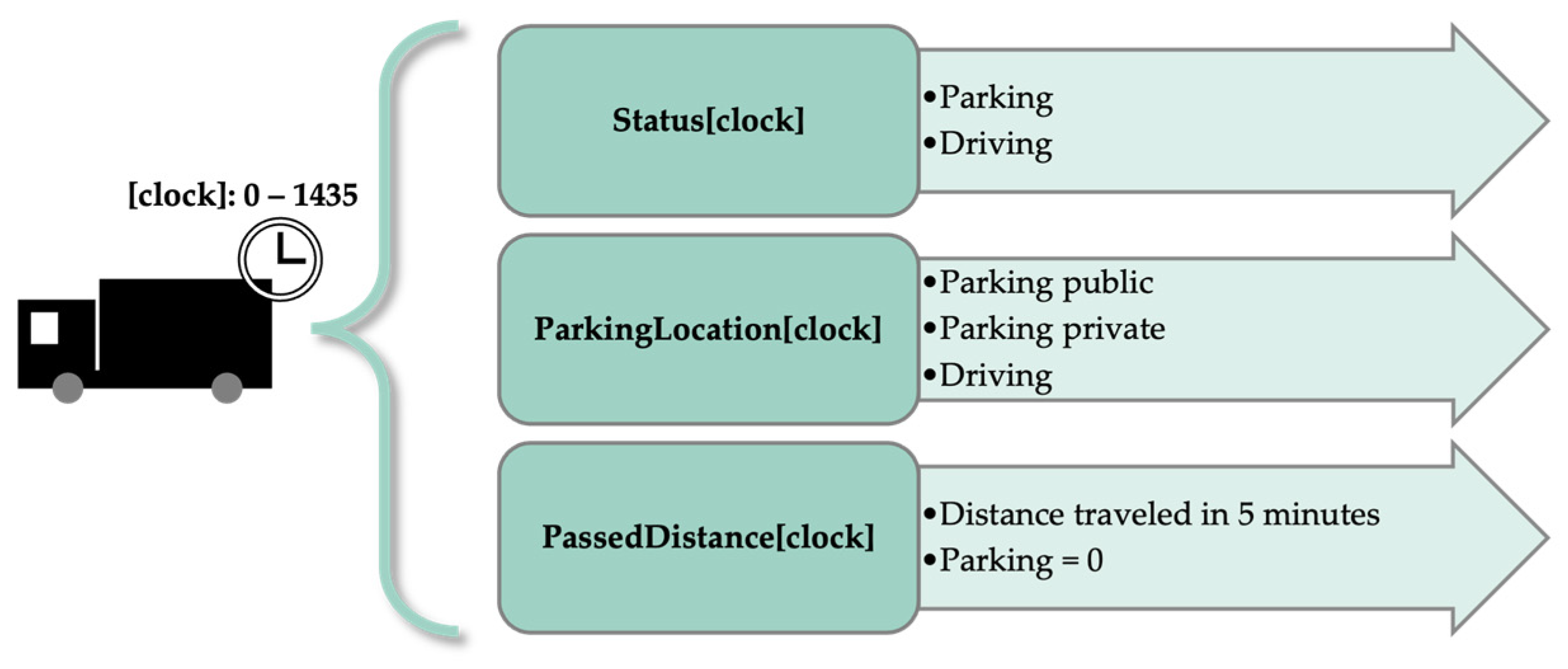
Based on these previous calculations, we simulate the driving behavior for each rigid truck and each tractor-trailer over the course of a day and save the information every five minutes from minute 0 (00:00) to minute 1435 (23:55). At any point in time, we know whether the vehicle is driving or whether and where it is parked, as well as the distance traveled. Figure 2 provides an overview of the available information for each 5 min timestamp for a specific vehicle.

In the next step, we simulate the single-day driving profiles as BET profiles. The charging demand of the vehicles is determined at each timestamp. The demand is based on the distance traveled in kilometers. For each timestamp, we know the distance traveled (in km) since the last charging event, as well as the SOC after the last charging event. Therefore, we can determine the kilometers that need to be recharged at every timestamp. In summary, we simulate the SOC at 5 min intervals, assuming a constant energy requirement per kilometer.

Charging events occur only during breaks already taken by conventional trucks in the original driving profiles. For a charging event to take place, two conditions must be met: (1) the break must last at least 30 min and (2) the SOC is below the minimum range or will be below it after the next trip. Additionally, charging events are always scheduled after the last trip of the day.

In addition to the charging behavior, the simulation is similar to the one performed in [18]. The charging process is guided by the specific strategy in use. As described in Section 2.1.1, we define three different charging strategies: (1) as slow as possible (ASAP), (2) as fast as possible (AFAP), and (3) Combination.

The procedure for ASAP charging is summarized in the following description.

Program description ASAP timestamp t = departure first trip/5; each timestamp reflects 5 min with t0 = 00:00 and t287 = 23:55 SOC = 1 1. Check for charging occasion:      IF t = departure first trip/5 + 287:              FINISH EXECUTION; simulation for 24 h has finished      ELSEIF (status[t] = parking) AND (status[t − 1] = driving):              Examine necessity of charging event      ELSE: $SOC=SOC-{\displaystyle \frac{travelled distance in t \left[\mathrm{k}\mathrm{m}\right]\times energy consumption\left[\frac{\mathrm{k}\mathrm{W}\mathrm{h}}{\mathrm{k}\mathrm{m}}\right]}{Maximum range \left[\mathrm{k}\mathrm{m}\right]\times energy consumption\left[\frac{\mathrm{k}\mathrm{W}\mathrm{h}}{\mathrm{k}\mathrm{m}}\right] }}$              t = t + 1              Check for charging occasion 2. Examine necessity of charging event:      IF ((duration of stop ≥ 30 min) AND (SOC after next trip < minimum range)) OR (final stop):              Calculate charging power      ELSE:              t = t + 1              Check for charging occasion 3. Calculate charging power: $\mathit{charging} \mathit{per} \mathit{timestamp}=\mathit{min}(\mathit{maximum} \mathit{charging} \mathit{power},\frac{1-\mathit{SOC}}{\mathit{duration}\mathit{of}\mathit{stop}})[\mathrm{k}\mathrm{W}]\times \frac{1}{12}[\mathrm{h}]$      t = t + 1      Execute charging 4. Execute charging:      IF (SOC < 1) AND (status[t] = parking): $\mathit{SOC}=\mathit{SOC}+\frac{\mathit{charging} \mathit{per} \mathit{timestamp}\left[\mathrm{k}\mathrm{W}\mathrm{h}\right]}{Maximum range \left[\mathrm{k}\mathrm{m}\right] \times energy consumption\left[\frac{\mathrm{k}\mathrm{W}\mathrm{h}}{\mathrm{k}\mathrm{m}}\right]}$              t = t + 1              Execute charging      ELSEIF (SOC = 1) AND (status[t] = parking):              t = t + 1              Execute charging      ELSEIF status[t] = driving:              Check for charging occasion

The procedure for AFAP works similarly to the ASAP procedure, except for the determination of the charging speed (step 3 in the program description). While ASAP calculates the minimum charging power necessary, AFAP uses the maximum power available. The modified program description (step 3) is given below:

Program description AFAP, step 3 3. Calculate charging power: $charging per timestamp=maximum charging power\left[\mathrm{k}\mathrm{W}\right]\times {\displaystyle \frac{1}{12}}[\mathrm{h}]$       t = t + 1      Execute charging

The calculation of the Combination strategy follows the logic that slow depot charging, as in the ASAP strategy, is combined with fast public charging, as in the AFAP strategy. Again, the modified program description (step 3) is given below:

Program description Combination, step 3 3. Calculate charging power:      IF parking location (t) = public: $charging per timestamp={maximum charging power}_{public}\left[\mathrm{k}\mathrm{W}\right]\times {\displaystyle \frac{1}{12}}[\mathrm{h}]$      ELSEIF parking location (t) = private: $charging per timestamp={min(maximum charging power}_{private,}\frac{1-\mathit{SOC}}{\mathit{duration}\mathit{of}\mathit{stop}})\left[\mathrm{k}\mathrm{W}\right]\times {\displaystyle \frac{1}{12}}[\mathrm{h}]$      t = t + 1      Execute charging

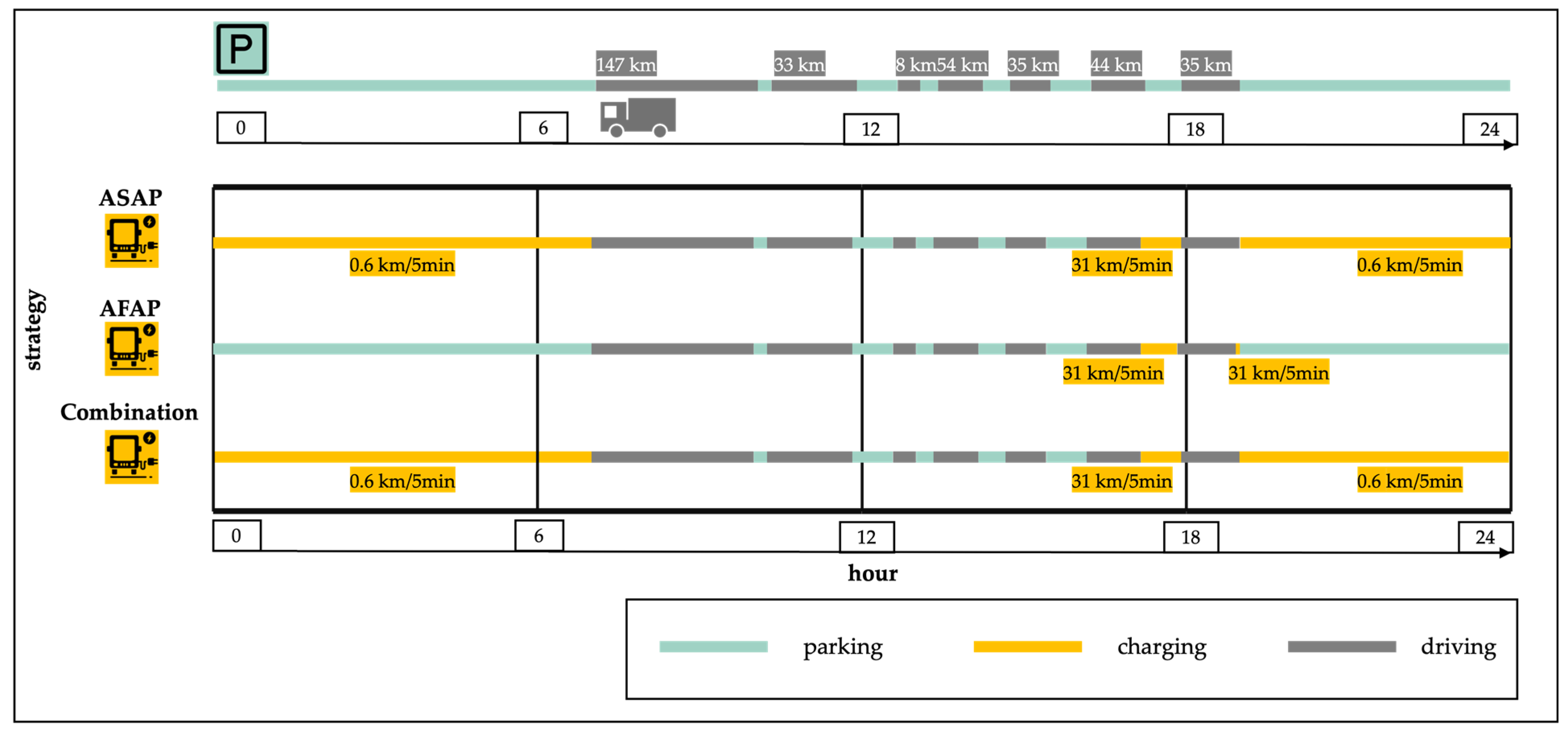
Simulations are conducted for each strategy–year scenario using the specific technical parameters. Figure 3 shows an exemplary driving profile for the year 2030. The vehicle starts driving at 7:00. After six trips and 321 km, the vehicle recharges at a public location. In 45 min, 280 km are recharged, which equals the maximum average charging power of 2030. As the vehicle cannot fully recharge during this first charging stop and therefore charges at the maximum possible charging power, the ASAP and the Combination strategies are identical in this case. After another trip, the vehicle arrives at its depot. Depending on the charging strategy, the vehicle is either charged slowly overnight or as fast as possible from the moment of arrival.

A driving profile is deemed to be feasible if the required range is not higher than the maximum possible range of the battery electric model in the corresponding year and if the vehicle can be recharged after the last trip before the first trip on the next day starts. In other words, a conventional HDV cannot be replaced by a BET if a single trip exceeds the maximum range for a specific year, or if the combined distance of multiple trips exceeds the maximum range and the vehicle cannot be sufficiently recharged during the stops.

Finally, the profiles are scaled for the total electrified truck fleet, considered in the corresponding year. By 2030, one-third of all vehicles are assumed to be electric vehicles. Depending on the charging strategy, the scaling factor varies, as a different number of driving profiles are feasible under different charging strategies. However, the total number of electrified trucks remains constant. By 2045, the number of electric trucks varies between the different strategies, depending on the share of the fleet that can be electrified.

4. Results

In the following section we provide an overview of the parking and driving behavior of the simulated vehicles (Section 4.1 and Section 4.2). Afterwards, the resulting load profiles are presented (Section 4.3). Finally, a sensitivity analysis is shown (Section 4.4).

4.1. Overview on Driving and Charging Behavior

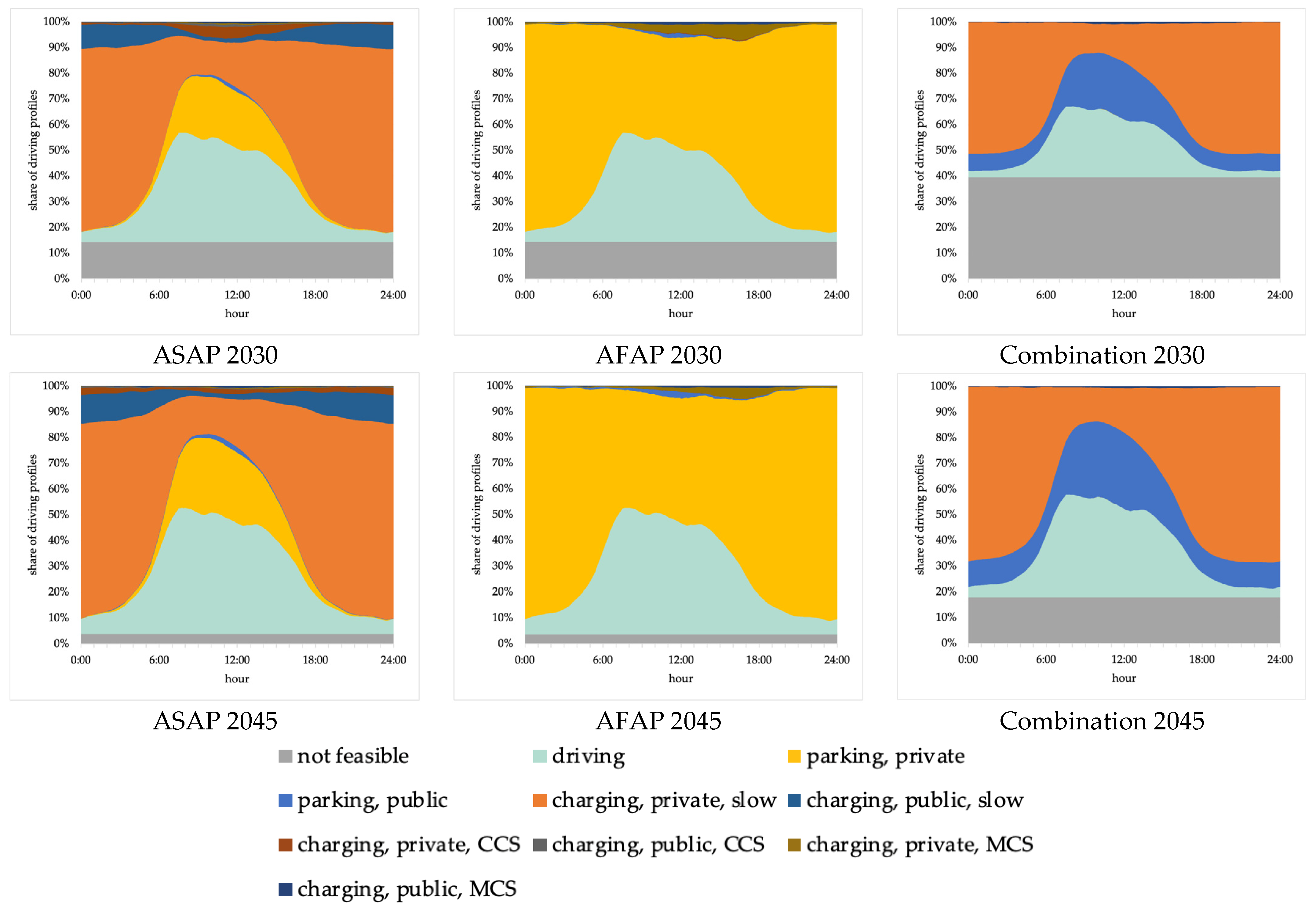
Figure 4 provides an overview of the activities of the fleet during the day, smoothed over a one-hour period. The shape of the curve for the driving profiles remains quite consistent across all strategies and years. In the morning, the share of vehicles on the road increases, peaking between 7:00 and 13:00, before gradually declining.

When using the ASAP strategy, charging at up to 44 kW—mainly at private locations—dominates, accompanied by a smaller share of charging processes with higher power. Looking at the AFAP strategy, most charging events take place at private locations with MCS charging. Afterwards, the vehicles remain parked throughout the night without charging. In the Combination strategy, private charging events with power levels up to 44 kW play the most significant role. Due to the assumption that vehicles use MCS at public charging stations, a significant share of vehicles remains parked without charging in public areas. By 2045, this affects up to 30% of vehicles at the same time. However, the lack of private charging infrastructure with higher power levels than 44 kW results in a higher share of vehicles that cannot be electrified.

4.2. Technical Feasibility and Number of Charging Events

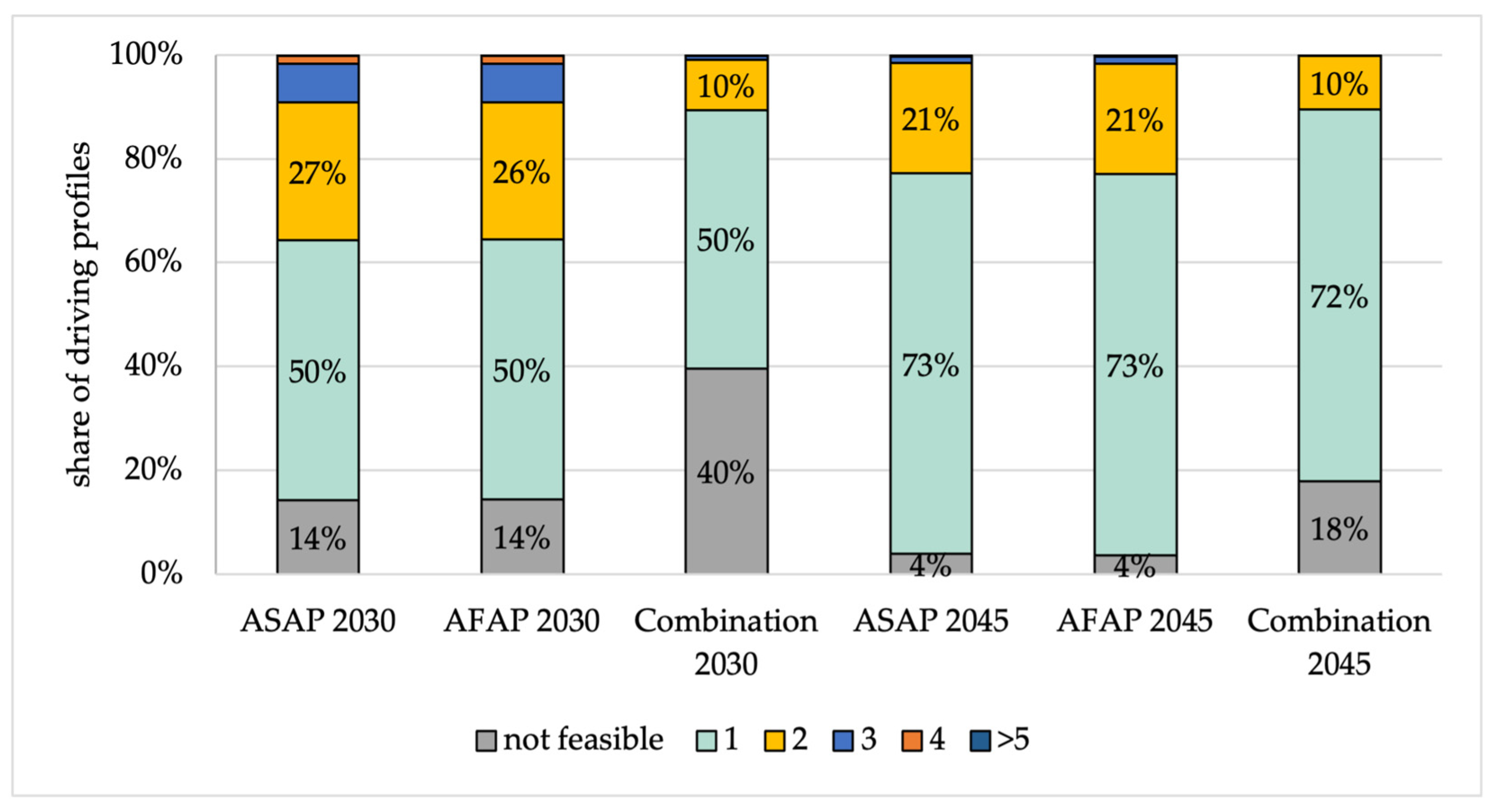
Due to the limited charging power and charging time, some conventional driving profiles cannot be completed with BET. While their share is comparatively low in the ASAP and AFAP strategies (14% in 2030, 4% in 2045), the Combination strategy counts 40% non-electrifiable driving profiles in 2030 (18% in 2045). The main reason is the limited charging power at the depot (max. 44 kW), which prevents the vehicles from being fully recharged.

As shown in Figure 5, one (overnight) charging event per day is enough to electrify half of the fleet in 2030. By 2045, the share increases to almost three-quarters of the fleet. In the ASAP and AFAP strategies, the proportion of required charging stops decreases significantly between 2030 and 2045. While 36% of battery-electric driving profiles require at least two charging stops in 2030, this proportion falls to 23% in 2045. In the Combination strategy, the proportion of driving profiles requiring more than one charging stop per day remains at roughly the same level over the years (10%), mainly due to the inability to electrify a large share of long-haul profiles.

Additionally, the share of driving profiles that rely at least partly on public MCS charging is examined. The specific shares in 2030 and 2045 vary only slightly across all strategies. In the ASAP strategy, the shares are in the range of 10%, while for the two other strategies they are in the range of 20 to 25%. This difference arises from the assumption that vehicles charge as slow as possible in the ASAP strategy. Fast charging, particularly MCS charging, is only needed in rare cases. It should be noted that public MCS charging involves only a minority of all charging events. However, MCS charging events are highly relevant for enabling long-haul trucking.

4.3. Load Profiles

To get an understanding of the potential impact of electrifying the German HDV fleet on the energy system, our driving profiles are extrapolated to a possible future BET fleet size. The additional energy required is determined and the power demand throughout the day is discussed.

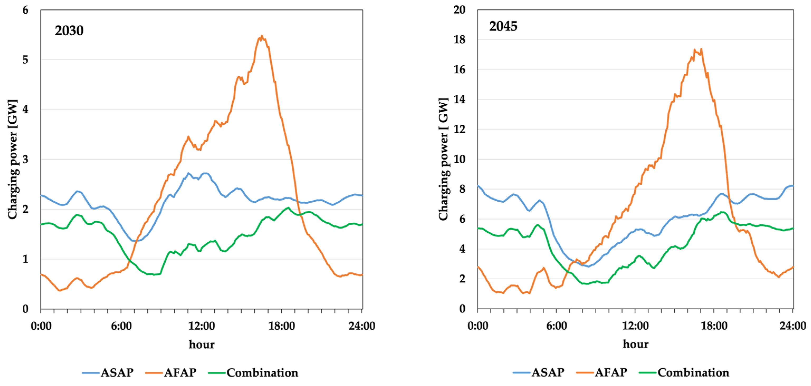
Figure 6 shows the load profiles in 2030 and 2045. The AFAP strategy leads to peaks in midday and evening hours. The midday peak is due to intermediate charging, while the evening peak results from charging for the next day. With a charging power of 6 GW in 2030, the peak value reaches almost 10% of today’s usual power demand in Germany. In 2045, the peak reaches 18 GW. The ASAP and Combination strategies have a much lower power demand. ASAP is always higher than Combination. As it is assumed that one-third of the fleet is electrified in 2030, the fleets are not identical in the scenarios. The Combination strategy mainly involves electrifying vehicles with below-average mileage, which results in lower total energy demand (36 GWh/day vs. 52 GWh/day). In 2045, the share of electrified vehicles and their energy demand using the Combination strategy is lower than using the other strategies (82% vs. 96%, 145 GWh/day vs. 103 GWh/day).

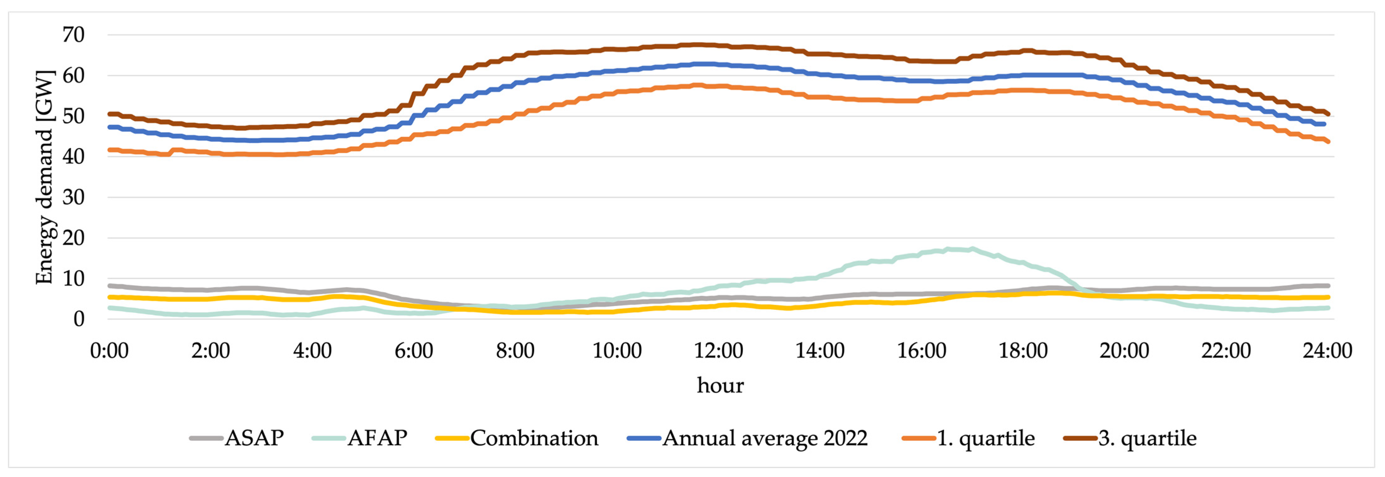
For comparison, Figure 7 shows the additional load for the defined charging strategies and the average electricity load curve in 2022. Even though electricity demand will increase in the future, BETs will generate relevant demand and need to be considered in energy system modeling.

4.4. Sensitivity Analysis and Monte Carlo Simulation

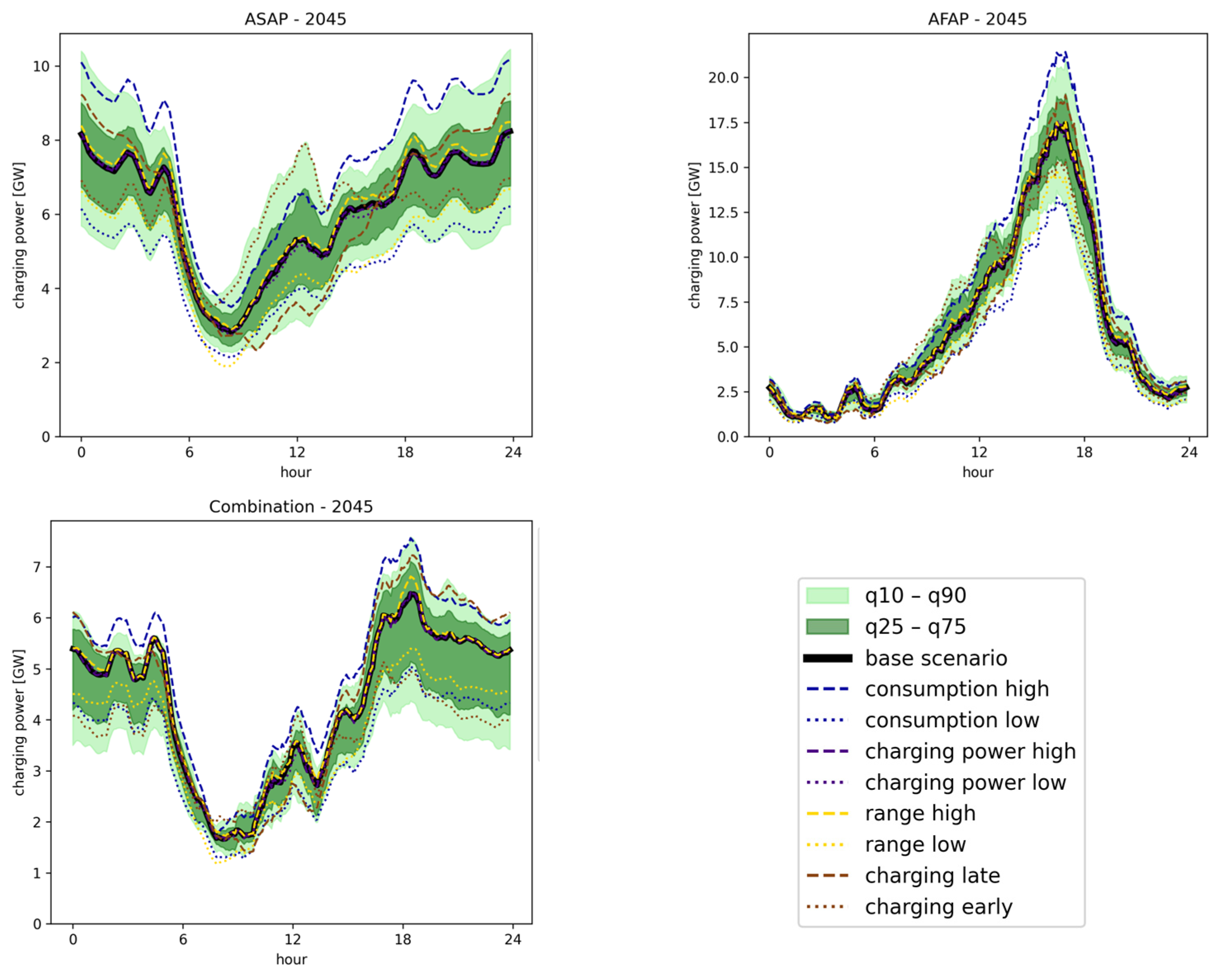
To evaluate the robustness of the simulated load profiles, we varied the most relevant parameters by plus/minus 25%. The variation in energy consumption can represent, for example, the effect of bad weather and the associated higher energy consumption. The maximum available charging power, as well as higher and lower vehicle ranges, exemplify the effects of slower or faster technical development than originally assumed. Finally, the variation in charging time can be interpreted as more or less risk-averse route planning. The variation in charging time is implemented by triggering a charging event if the remaining range would fall below 60% on the next trip (charging early) or if the battery would actually run out (charging late). In addition to the ceteris paribus variations, a Monte Carlo simulation was performed for each of the three charging strategies. In total, 100 randomly selected combinations of the mentioned parameters were calculated for each strategy, varying the parameter by up to plus/minus 25%. Figure 8 shows the results of the sensitivity analysis and the Monte Carlo simulation.

The variation in energy consumption shifts the load curve, particularly along the y-axis. Higher energy consumption leads to a higher overall load curve. The influence of the charging power is limited.

When charging as slow as possible, additional charging power is not needed to fulfill the logistics tasks; the available charging power in the base case is already (more than) sufficient. When charging as fast as possible, the charging events of single vehicles are already quite short, typically less than 30 min. Higher charging power leads to even shorter charging times. While the additional charging power extends the peak demand in a specific timeframe, the shorter charging time reduces the peak in the next timeframe. Focusing on the whole fleet, the total load curve remains almost constant, as not all vehicles arrive at the same time.

Reducing the range partly makes electrification more complicated so that less vehicles are electrified, leading to a lower load curve. However, ranges greater than the base case only led to minimal gains in terms of technical feasibility and therefore have little effect on the load curve.

Earlier recharging increases demand in the morning and midday hours and reduces demand in the evening and night hours.

5. Discussion

In the following relevant assumptions, the model itself and the results are briefly discussed.

The energy consumption of the vehicles is a relevant input parameter. It depends on weather conditions, road conditions, individual driving behavior, and the design and the weight of the vehicle. Higher or lower consumption can also affect the vehicle range. A higher range would reduce the demand for intermediate charging, and therefore the midday charging demand. Conversely, a lower range would increase the intermediate charging demand. However, as our range assumptions are rather conservative, higher demand would potentially lead to longer ranges (and larger batteries). Therefore, the charging behavior would remain similar, while the overall energy demand would increase linearly with the additional energy consumption.

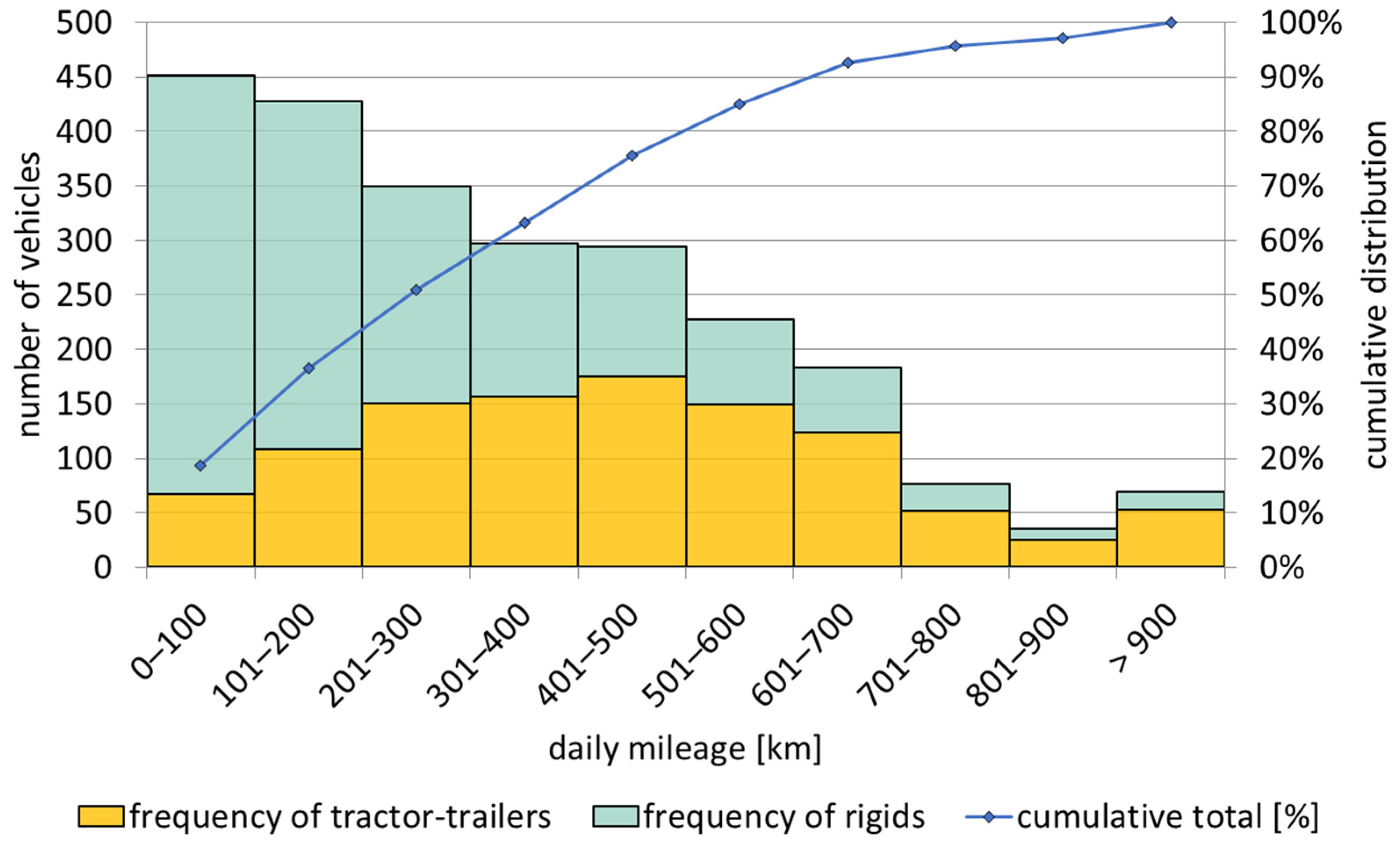
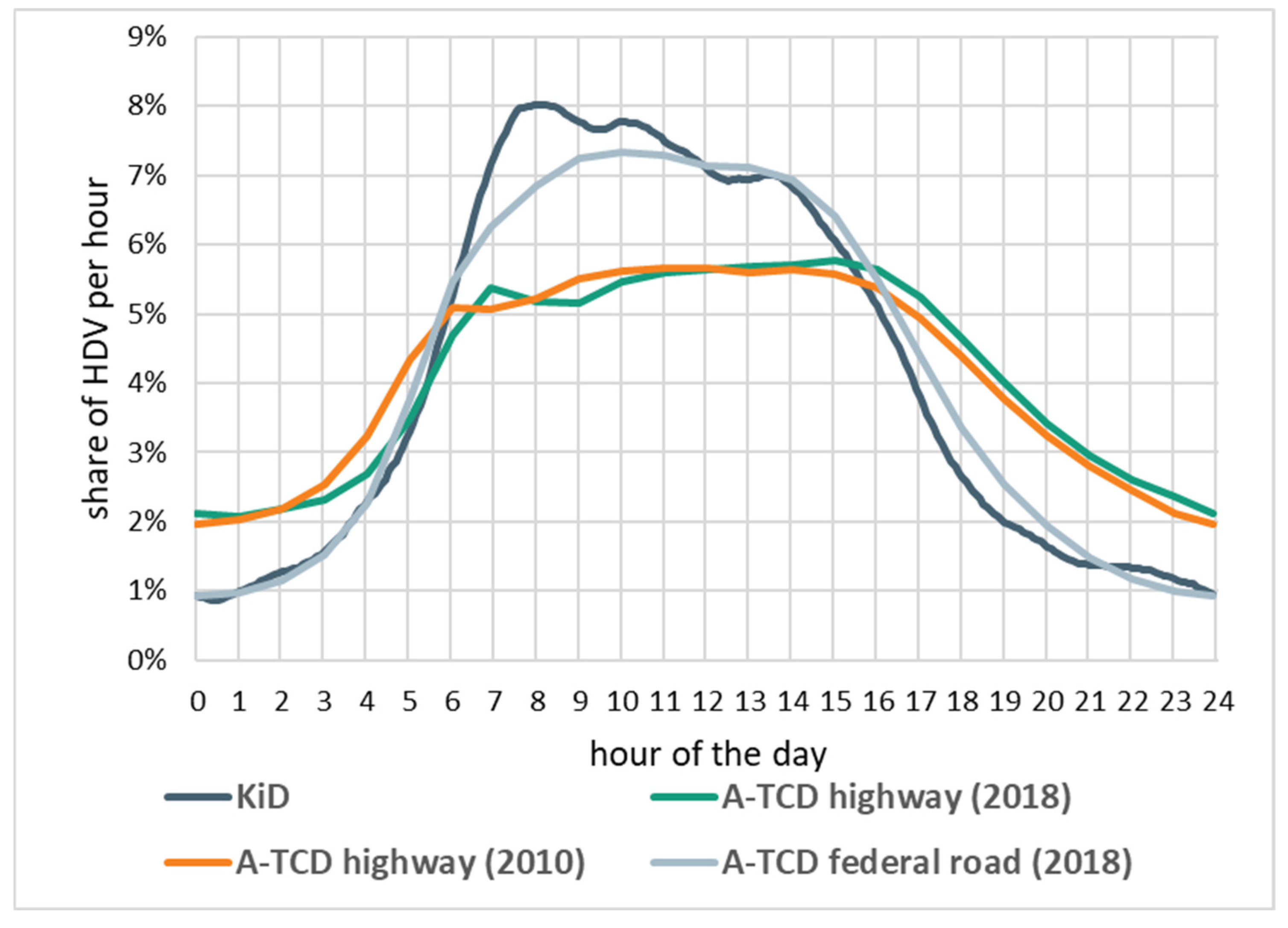
Another limitation is given by our driving profile data. There is only a limited number of driving profiles, and the trip data is recorded by hand. Even though the dataset has a high consistency with German traffic count data and is therefore deemed to be representative [18], future analysis should include additional driving profiles. In particular, the comparison with traffic count data in Appendix A shows that regional traffic is very well represented, while long-distance traffic is structurally included but may be proportionally slightly too small. In the future, new data could show changes compared to the KiD data from 2010 and enable an even more detailed calculation of charging requirements. Additional geographic information (GPS coordinates) could improve the identification of suitable charging locations, compared to the pure differentiation between public and private locations. This information would enable an assessment of the impact on specific regional network nodes, including potential overload risks, rather than limiting the analysis to time-resolved effects on the overall load.

While our data reflects driving behavior at a single point in time, logistics constantly change. New trends—e.g., growing e-commerce, new logistics concepts, and (partially) autonomous driving—will change HDV operation. Analyses show that there is already potential for optimization with the technology available today [29]. At the same time, it is uncertain how quickly and to what extent the mentioned innovations will influence driving behavior. Future simulations should include corresponding scenarios.

Our assumptions of the future BET fleet are based on the literature and the technical feasibility calculated in our analysis. A smaller or higher penetration of BETs would linearly influence the load profiles.

The implemented charging strategies simplify the scheduling of charging events by triggering them based on the SOC. Since most truck traffic is scheduled, one might assume that charging events will be integrated into the trip planning process. This may slightly affect the results. For example, there are stops shortly before arriving at a depot. In such cases, a logistics company will likely reschedule the trip or select a vehicle with a slightly higher range. This means that our analysis potentially overestimates the need for public and intermediate charging.

The load curves of potential strategies generated in this paper offer an overview of their impact under simplified assumptions. To assess their practical applicability, we evaluate these strategies with a focus on meeting the diverse requirements and needs of different stakeholder groups: (1) Logistics companies and fleet operators prioritize minimizing the likelihood of waiting times. To achieve this, the AFAP strategy is highly suitable, as it charges vehicles as fast as possible, thereby keeping charging stations available for subsequent charging processes. Additionally, these stakeholders aim to reduce the number of charging events per trip, enhancing route plannability [30] and avoiding detours to reach charging points. (2) For grid operators, however, it is very crucial to understand the vehicles’ energy requirements and to prepare the grid accordingly. A strategy that ensures relatively even load distribution and limits demand during national peak electricity times is ideal. Both the ASAP and Combination strategies meet these requirements. AFAP, in contrast, causes additional load peaks and is therefore rather unsuitable for widespread application. When it comes to implementation, the Combination strategy is the most feasible one, as it combines both objectives: flattening the load curve and minimizing waiting and charging times during trips. (3) Another stakeholder group consists of policy makers. Funding is needed to set up charging infrastructure. To make well-informed, long-term decisions, it is important to understand where and when different load capacities are required.

In line with the primary objective of this study, the extreme strategies (AFAP and ASAP) were selected to demonstrate the full range of possible impacts on the load curves. Our results indicate that a well-developed private slow charging infrastructure will form the backbone of future electrified truck traffic. However, long-distance transport in particular will rely on both public and private high-power charging infrastructure.

When assessing the feasibility of individual driving profiles, sufficient charging infrastructure availability is assumed, with neither competition for charging points nor waiting times. This simplification is made because realistic assumptions about future charging infrastructure are subject to considerable uncertainty, as they would require detailed knowledge of the capacity and spatial distribution of charging stations that does not yet exist. Any resulting waiting times would shift the load curve but would not affect the overall load curve.

Moreover, this analysis focuses only on the technical feasibility and the impact on the load curve, while economic aspects are not modeled here. When interpreted in combination with the studies by Samet et al. [8], implications for the economic performance of different charging strategies can be evaluated. The pure acquisition and hardware costs for BET infrastructure play a much smaller role than the opportunity costs associated with en-route charging. These include, e.g., driver wages and insurance costs due to extended working hours and lost profits due to necessary breaks for charging [8]. Especially in long-distance transport, the economic efficiency of BET operation is strongly influenced by the possibility of minimizing charging time on the road and the associated opportunity costs. However, a more detailed calculation of the costs incurred by the various stakeholder groups could be the subject of future research.

Another aspect not considered in this work, but holding great potential for future research, is the application of intelligent charging methods and bidirectional charging, also known as “vehicle-to-X” (V2X). This involves the integration of electric vehicles into the power grid. Initial case studies suggest technical and economic feasibility [31,32]. In smart charging scenarios, different targets can result in different operational and charging decisions, leading to different patterns of charging loads [33]. For example, it is possible to minimize grid connection or participate in various energy markets. However, the integration of V2X requires extensive further data collection and assumptions that would exceed the scope of this study.

6. Conclusions

We simulate all daily trips of 2410 trucks in Germany as BETs and apply three different charging strategies. To provide initial insights into potential effects of truck electrification on the energy system, we find that a full fleet conversion can lead to additional load peaks. By 2030, BETs may cause an additional load of up to 6 GW (10% of the average load in Germany), if charging is not properly managed. However, if slow charging is applied, peaks are approximately halved. Compared to immediate fast charging, slow charging shifts energy demand from early evening hours to nighttime hours. By 2045, the additional demand may increase to 18 GW under the fast charging strategy and 8 GW under the slow charging strategy. Our results provide initial insights for (1) logistics companies to plan their private charging infrastructure, (2) grid operators and energy providers to prepare their infrastructure, and (3) politicians to support a suitable infrastructure ramp-up.