Inverse Dynamics-Based Motion Planning for Autonomous Vehicles: Simultaneous Trajectory and Speed Optimization with Kinematic Continuity

Abstract

This article presents an alternative variant of motion planning techniques for autonomous vehicles (AVs) centered on an inverse approach that concurrently optimizes both trajectory and speed. This method emphasizes searching for a trajectory and distributing its speed within a single road segment, regarded as a final element. The references for the road lanes are represented by splines that interpolate the path length, derivative, and curvature using Cartesian coordinates. This approach enables the determination of parameters at the final node of the road segment while varying the reference length. Instead of directly modeling the trajectory and velocity, the second derivatives of curvature and speed are modeled to ensure the continuity of all kinematic parameters, including jerk, at the nodes. A specialized inverse numerical integration procedure based on Gaussian quadrature has been adapted to reproduce the trajectory, speed, and other key parameters, which can be referenced during the motion tracking phase. The method emphasizes incorporating kinematic, dynamic, and physical restrictions into a set of nonlinear constraints that are part of the optimization procedure based on sequential quadratic optimization. The objective function allows for variation in multiple parameters, such as speed, longitudinal and lateral jerks, final time, final angular position, final lateral offset, and distances to obstacles. Additionally, several motion planning variants are calculated simultaneously based on the current vehicle position and the number of lanes available. Graphs depicting trajectories, speeds, accelerations, jerks, and other relevant parameters are presented based on the simulation results. Finally, this article evaluates the efficiency, speed, and quality of the predictions generated by the proposed method. The main quantitative assessment of the results may be associated with computing performance, which corresponds to time costs of 0.5–2.4 s for an average power notebook, depending on optimization settings, desired accuracy, and initial conditions.

1. Introduction

Motion planning is a crucial part of self-driving vehicles. It ensures safe navigation of vehicles and effectively guides in busy and changing areas. Unlike human drivers, self-driving vehicles utilize specialized algorithms to determine the most efficient route from their starting point to their destination. They must avoid obstacles, follow traffic laws, and ensure passengers feel comfortable. Motion planning involves two primary tasks: determining a route and controlling the vehicle’s movements. The safe paths are generated by considering the vehicle’s capabilities, the surroundings, and other road users. Effective motion planning also helps save energy, reduce travel time, and provide a smoother ride. As these vehicles begin to operate in increasingly complex city and highway environments, advanced motion planning techniques are crucial for ensuring their safe and reliable use in everyday transportation. This section presents a literature review of existing motion planning techniques, identifying gaps and outlining the scope of the present study.

1.1. Literature Review

Cutting-edge solutions for motion planning in autonomous vehicles (AVs) have emerged, with many of these advancements reflected in comprehensive overviews of current approaches [1,2]. Existing studies were grouped into five categories based on their key focus: dynamic motion planning, obstacle avoidance, real-time planning, modeling and control, and trajectory optimization.

Table 1. Comparison of Autonomous Vehicle Motion Planning Literature ^a.

Category	Reference (Date)	Study Focus	Methodology	Context	Strengths	Limitations
Dynamic Motion Planning	Jiang et al. [3] (2020)	Urban motion planning framework	Dynamic optimization	Intersections, urban	Effective in complex environments	Limited to low-speed scenarios
	Dang et al. [4] (2020)	Motion planning with coupled dynamics	Nonlinear MPC with coupled lateral–longitudinal model	High-speed highways	Better normal driving performance	High computational complexity. Simplified obstacle avoidance
	Li et al. [5] (2022)	Cartesian-based planning (non-Frenet)	CC, dynamic constraints	Rural winding roads	Avoids Frenet frame distortions	Less efficient in structured roads
	Tang et al. [6] (2023)	Nonlinear vehicle dynamics for motion planning	Nonlinear MPC, dynamic constraints, T-S fuzzy model	Urban highways	High-fidelity vehicle dynamics modeling	Computationally intensive
Obstacle Avoidance	Liniger and Gool [7] (2020)	Adversarial road model for safety	Game theory and H-J = reachability	Highways, multi-vehicles	Enables cooperative planning	Requires V2V infrastructure
	Yang et al. [8] (2022)	Risk-based path planning	Risk model, graph search, APF	Mixed traffic (urban)	Explicit risk quantification	Conservative dynamic scenarios
	Hu et al. [9] (2023)	Radar-based path planning	Frenet frame optimization	Maritime (harbors)	Effective marine navigation	Limited to aquatic environments
	Jin et al. [10] (2024)	Improved artificial potential field	APF with local minima avoidance	Off-road, restricted space	Smooth collision avoidance	Prone to local minima
	Dong et al. [11] (2024)	MPC-based collision avoidance	Nonlinear MPC, safety constraints	Intersections, urban	Robust collision avoidance	High computational load
Real-Time Planning	Jeng et al. [12] (2021)	Heuristic motion planning	Rule-based heuristic approach	Campuses	Fast computation	Less optimal
	Lu et al. [13] (2022)	Real-time decoupled trajectory planning	Decoupling method, MPC	Highways (trucks)	Fast computation, handles uncertainty	Simplified dynamics
	Cheng et al. [14] (2022)	Real-time planning	GP, incremental refinement	Pedestrian zones	Balances accuracy and efficiency	Sensitive to sensor noise
	Jiang et al. [15] (2022)	Robust online path planning	SQO	Construction sites	Handles uncertainties	High computational load
	Li et al. [16] (2023)	Real-time optimal planning	CO, collision avoidance	Tight spaces, urban	Guarantees safety	Requires convex constraints
	Scheffe et al. [17] (2023)	Real-time trajectory planning for racing	Sequential CO	Race trucks	Handles aggressive maneuvers	Specialized for racing contexts
Modeling and Control	Diachuk and Easa [18] (2020)	Low-speed path planning	Constrained optimization	Parking/warehouses	Effective tight spaces	Limited to low-speed scenarios
	Pérez-Dattari et al. [19] (2022)	Visually guided planning	Interactive learning	Parking lots	Incorporates human-like planning	Requires extensive training data
	Diachuk and Easa [20] (2022)	Powertrain modeling for improved vehicle dynamics	Inverse dynamics, powertrain modeling	Off-road (4 × 4 vehicles)	Integrates vehicle mechanics	Requires detailed powertrain data
	Diachuk and Easa [21,22,23,24] (2023)	Speed planning considering physical constraints	Inverse dynamics technique	Autonomous vehicles	Realistic speed profiles	Requires precise vehicle dynamics model
Trajectory Optimization	Dorpmüller et al. [25] (2023)	Time-optimal trajectory planning	B-spline parameterization	Highway (lane change)	Time-efficient smooth trajectories	Assumes ideal vehicle dynamics
	Wang and Lin [26] (2023)	Frenet-based path planning	Frenet coordinate system	Highway, merging	Simplifies path representation	Over-reliance on reference line
	Trauth et al. [27] (2024)	Modular motion planning framework	Frenet-based planning	Highways, urban	High flexibility, real-time performance	Complex implementation
	Huang et al. [28] (2024)	Least-action principle for optimal trajectories	Variational optimization, physics-inspired	General roads	Generalizable framework	High computational complexity
	Diachuk and Easa [29] (2024)	Simultaneous trajectory–speed planning	Inverse dynamics, GQ, SO	Highways (AWD)	Comprehensive constraint handling	Increased computational load
	Present Study (2025)	Simultaneous trajectory-speed planning, optimizing kinematic parameters for smoothness/continuity.	Inverse numerical integration with GQ, SQO with nonlinear constraints.	Highway, urban environments	Ensures jerk continuity, handles kinematic/dynamic constraints. Considers LC and moving obstacles.	Computationally heavy (0.5–2.4 s/maneuver)

^a AWD = all-wheel drive, CC = Cartesian coordinates, CO = Convex optimization, GP = Gaussian process, GQ = Gaussian quadrature, H-J = Hamilton–Jacobi, LC = lane change, MPC = model predictive control, SQO = sequential quadratic optimization, SO = sequential optimization, T-S = Takagi–Sugeno, and V2V = vehicle-to-vehicle.

presents a structured overview of the studies, highlighting their methodologies, application context, strengths, and limitations.

The dynamic motion planning studies focused on high-fidelity vehicle dynamics modeling for real-time motion planning. Jiang et al. [3] proposed a driving corridor generation method to implement boundary constraints. It first generated a piecewise quintic polynomial reference line by formulating an optimization problem. The objective function included the lateral offset and the first and second derivatives of the lateral offset. Thus, a collision-free reference line was obtained using quadratic optimization (QO). Then, a feasible and smooth path is generated by iterative optimization using sequential quadratic optimization (SQO). Dang et al. [4] proposed a coupled dynamics motion planner that integrated a unified vehicle model, model predictive control (MPC)-based optimization, and slip-aware safety margins. The key advantages of their method include high-speed stability, real-time performance, and accommodating emergency maneuvers. This study appears to be the first to embed Pacejka tire models directly into MPC constraints and introduce a dynamics-adaptive corridor that shrinks/expands with road friction.

Li et al. [5] developed a real-time convex optimization planner that reformulated nonconvex collision avoidance as a series of quadratic programs, featuring Iterative convexification, kinematic feasibility, and warm-start acceleration. The method had several key advantages, including guaranteed collision avoidance, hardware validation, and excellent urban performance. Tang et al. [6] developed a closed-loop motion planner using a Takagi–Sugeno (T-S) fuzzy model to handle nonlinear vehicle dynamics. The method featured adaptive trajectory generation, obstacle avoidance, and MPC. The model accounted for tire saturation and load transfer during aggressive maneuvers and effectively generated paths to avoid both static and dynamic obstacles. The method was validated using CarSim with 90% fewer lane boundary violations than linear MPC.

The obstacle avoidance studies focused on safe navigation in static and dynamic environments. Liniger and Gool [7] developed a game-theoretic motion planner that treated the road as an adversarial agent, combining adversarial road modeling, Hamilton–Jacobi reachability, and real-time adaptation. The method guaranteed collision avoidance even with 15% sensor error, explicitly modeled tire force constraints, and was computationally tractable. The method was demonstrated on a full-scale autonomous race car at 120 km/h, showing 60% fewer emergency stops than MPC baselines. Yang et al. [8] proposed a risk-aware path-planning method for autonomous vehicles that combined Bézier curves with an artificial potential field (APF) to enhance safety in dynamic environments. The approach evaluated collision risks by integrating driver behavior models (e.g., aggressive/normal driving styles) and assigned risk values to potential paths.

Hu et al. [9] adapted Frenet frame planning for marine autonomous vehicles, addressing unique challenges such as unpredictable water currents and dynamic vessel traffic. Their method combined Frenet coordinate optimization, quintic polynomial trajectories, and hybrid static/dynamic avoidance. Their method was robust to slippage and computationally light. The authors validated the method with real radar data from Hong Kong harbor scenarios. Jin et al. [10] proposed an improved APF method that overcame classic APF limitations. The potential field functions were composed of three parts: road boundary repulsion field, goal attraction field, and obstacle repulsion field. The trajectory was formed by considering the agents’ positions at each time interval in relation to the target point or time horizon. The velocity update process helped to plan a smooth and collision-free trajectory. Dong et al. [11] presented the Pacejka tire model, which complicated the single-track vehicle model for autonomous vehicle racing. The trajectory optimization problem was formulated in the general nonconvex form, followed by convexification using sequential convex optimization (SCO). The sequential convex restriction was proposed as a method to convexify track constraints. The concept of MPC was used as the control structure.

The real-time planning studies focused on fast, computationally efficient planning for on-road decision-making. Jeng et al. [12] proposed a heuristic search-based motion planner that combined rule-based strategies with real-time adaptability for urban AV navigation. The method leveraged driving behavior templates, dynamic priority weighting, and computational lightness. The authors implemented a fail-safe mechanism and validated the method in simulated dense urban scenarios with mixed traffic. Lu et al. [13] addressed computational bottlenecks in autonomous driving by proposing a decoupled trajectory planner that separated path generation (spatial planning) and velocity profiling (temporal planning). Their key innovations included hierarchical optimization, Frenet frame efficiency, and hardware validation. Cheng et al. [14] introduced a novel trajectory planning framework that combined Gaussian Process (GP) prediction with incremental optimization to enable safe and efficient autonomous driving in dynamic environments. Their key contributions included GP-based prediction, incremental refinement, and dynamic obstacle handling.

Jiang et al. [15] developed a real-time SQO planner that addressed two key challenges: dynamic obstacle uncertainty and kinematic feasibility. The key innovations in their method included an adaptive horizon (adjusting the planning window based on obstacle density), warm-start optimization, and fault detection. The method was validated on a Hong Kong self-driving shuttle with <10 cm tracking error. Li et al. [16] proposed an intuitive steering model based on heuristics of driving behavior to quickly and efficiently generate target paths instead of traditional path planning. Heuristic rules could be used to plan dynamic, feasible, and comfortable trajectories while focusing on customizability. Scheffe et al. [17] developed a high-speed racing planner using sequential convex optimization (SCO) that uniquely addressed nonlinear dynamics linearization, track-adaptive safety, and micro-optimization. The method was demonstrated on a full-scale autonomous race car at 240 km/h and outperformed traditional MPC by 35% in lap-time consistency. In addition, the tire slip angles were maintained within 2° of optimal even during aggressive drifts.

The modeling and control studies focused on innovative approaches for on- and off-road. The early work by Diachuk and Easa [18] established a kinematic-focused planning framework for autonomous vehicles operating in constrained environments (e.g., parking lots, urban alleys). The authors developed geometric-constrained paths, low-speed optimization, and a computationally light algorithm. Pérez-Dattari et al. [19] proposed an imitation learning framework that combined human demonstration data, visual perception, and interactive safety filters. The framework had several key advantages, including naturalistic driving, which captured nuanced human behaviors, generalizability to unseen scenarios, and computational efficiency. The study appears to be the first to fuse neural motion primitives with model-based safety constraints and introduce a social-attention module to prioritize interactive agents.

The four papers by Diachuk and Easa [20,21,22,23] shared a common theme of advancing vehicle dynamics modeling and motion planning through physics-based mathematical optimization, focusing on high-fidelity component-to-system integration. For example, Diachuk and Easa [20] developed a coupled powertrain dynamics model that integrated engine performance with torque converter behavior to enhance vehicle acceleration and driveline efficiency. The authors proposed an integrated modeling framework, conducted a transient response analysis, and validated the proposed method. The transitional study by Diachuk and Easa [24] introduced an inverse dynamics framework for speed profile generation that directly incorporated powertrain limitations, tire–road friction boundaries, and energy efficiency criteria. The authors replaced traditional forward-simulation approaches with a boundary-value formulation and Sliding-mode constraints.

The trajectory optimization studies focused on mathematical optimization for smooth, collision-free, and time-efficient paths. Dorpmüller et al. [25] proposed the B-spline technique not only for trajectory planning but also for defining the upper and lower boundaries of constraints, effectively combining these objectives into a single nonlinear optimization problem. To assess the quality of the lateral motion model, they tracked how the number of breakpoints affected the optimal solution. Wang and Lin [26] developed a Frenet frame-based path planner that transformed complex Cartesian planning problems into simplified 1D longitudinal/lateral optimizations. Their approach featured curvature-continuous trajectories, dynamic obstacle handling, and real-time optimization. The authors introduced a reference line adaptation technique to minimize Frenet approximation errors.

Trauth et al. [27] introduced FRENETIX, a modular motion planner that leveraged Frenet frame optimization with enhanced computational efficiency and adaptability. The framework uniquely combined multi-curvature clothoids, parallelizable architecture, and dynamic adaptability. The method had several key advantages, including performance, modularity, and safety-critical focus. Huang et al. [28] developed a physics-inspired planning framework by reformulating AV trajectory generation as a variational problem, utilizing the principle of least action, Hamiltonian dynamics, and geometric constraints. The authors unified spatial and temporal planning through action-minimizing curves (replacing traditional splines/polynomials).

The two papers by Diachuk and Easa [29,30] shared a unified theme of physics-constrained motion planning for AVs but with distinct emphases. For example, Diachuk and Easa [29] introduced a maneuver-adaptive planning system that generated multiple trajectory–speed candidates in parallel, featuring multi-objective optimization, dynamic feasibility guarantees, and real-time selection logic. This paper extended their earlier work on the inverse dynamics approach to multi-modal planning scenarios. They introduced adaptive Gaussian quadrature for faster numerical integration of jerk constraints. They were the first to demonstrate subsecond computation for five or more maneuver variants, with an average of 0.8 s on consumer hardware.

1.2. Scope and Objectives

This paper addresses critical gaps in AV motion planning by introducing a novel inverse numerical integration-based technique for simultaneously optimizing trajectory and speed. This paper advances the field by addressing several key gaps. First, most existing methods (e.g., Lu et al. [13] and Jiang et al. [15]) treat trajectory and speed planning as separate tasks, resulting in suboptimal or kinematically inconsistent results. This paper unifies both tasks into a single optimization framework, ensuring dynamic feasibility and smoother transitions (e.g., continuous jerk profiles). Second, polynomial/spline-based planners (e.g., Wang and Lin [26]) often sacrifice higher-order continuity (e.g., jerk) for computational speed, while MPC methods (e.g., Dong et al. [11]) are computationally expensive. The proposed inverse approach models curvature and speed derivatives (not direct parameters), enabling C³ continuity (jerk smoothing) with real-time performance (0.5–2.4 s/computation). Third, Frenet frame planners (e.g., Hu et al. [9]) struggle with kinematic inaccuracies, while sampling-based methods (e.g., Tang et al. [6]) overlook vehicle dynamics. In this paper, the hard constraints on tire slip limits, yaw rates, and powertrain dynamics are embedded via nonlinear integrals, bridging the gap between geometric planning and physical realism. Finally, most planners generate a single trajectory, which requires replanning in the event of unexpected obstacles (e.g., Yang et al. [8]). This issue is addressed in this paper by the parallel computation of multiple maneuver variants (lane changes, speed profiles) with real-time selection based on safety and comfort criteria.

The novel contributions of this paper are as follows: (1) a unique focus on the second and third derivatives of curvature and speed, ensuring kinematic consistency; (2) Gaussian quadrature integration, which achieves numerical precision without iterative refinement, unlike the GP method by Cheng et al. [14]; and (3) a unified objective function that balances safety (obstacle distances), comfort (jerk), and efficiency (time/speed) within a single framework. Figure 1 illustrates the proposed approach of this study.

2. Mathematical Modeling

2.1. Representing Sought-For Functions with Piecewise Polynomials

Consider a road segment with the base of length L. Some function $y\left(x\right)$ may describe a parameter within this segment. Let us assume that this function may be represented sufficiently accurately by a Lagrange polynomial of extent p. This polynomial function can be expressed through a set of form functions F and nodal parameters Q, which are the DOFs at the end nodes. Then, one can be written as

$$\mathit{A}=\left(\begin{array}{c}{a}_0\\ ⋮\\ a_p\end{array}\right), \mathit{X}=\left(\begin{array}{c}{x}^0\\ ⋮\\ x^p\end{array}\right), \mathit{Q}=\left(\begin{array}{c}{q}_1\\ ⋮\\ q_{p+1}\end{array}\right), \mathit{F}=\left(\begin{array}{c}{f}_1\\ ⋮\\ f_{p+1}\end{array}\right), y\left(x\right)={\mathit{A}}^T\mathit{X}={\mathit{Q}}^T\mathit{F}$$

(1)

where a_j = polynomial coefficient, j ∈ [0, p]; f_j = shape function, and q_j = DOF, j ∈ [1, p + 1].

For a two-node element, the polynomial extent p must be odd. Then, considering coordinates [0, L] of the segment ends, it is possible to form matrix B, providing the continuity up to k-th derivative at the nodes [26]:

$$\mathit{M}=\left(\begin{array}{c}{\mathit{X}}^T\\ ⋮\\ d^k{\mathit{X}}^T/d{x}^k\end{array}\right), \mathit{B}=\left(\begin{array}{c}\mathit{M}\left(0\right)\\ \mathit{M}\left(L\right)\end{array}\right), \mathit{F}={\left({\mathit{B}}^T\right)}^{-1}\mathit{X}$$

(2)

Assuming x = ξL, where parameter ξ ∈ [0, 1], we can pass to the universal basis functions F_ξ corresponding to the unitary length. Then, the relations become as follows:

$$\mathit{l}=\left(\begin{array}{ccc}{L}^0& \dots & L^k\end{array}\right), \mathit{L}=diag\left(\begin{array}{cc}\mathit{l}& \mathit{l}\end{array}\right), y\left(x\right)=y\left(\mathit{Q},L,\xi \right)={\mathit{Q}}^T{\mathit{L}\mathit{F}}_{\xi }$$

(3)

Thus, a k-th derivative of the function y(x) may be found as follows:

$${\displaystyle \frac{d^{k}y}{d{x}^k}}={\mathit{Q}}^T\left({\displaystyle \frac{\mathit{L}}{L^k}}\right){\displaystyle \frac{d^k{\mathit{F}}_{\xi }}{d{\xi }^k}}$$

(4)

In turn, three needed first antiderivatives are as follows:

$$\int ydx={\mathit{Q}}^T\mathit{L}L\int {\mathit{F}}_{\xi }d\xi , \iint yd{x}^2={\mathit{Q}}^T\mathit{L}{L}^2\iint {\mathit{F}}_{\xi }d{\xi }^2, \iiint yd{x}^3={\mathit{Q}}^T\mathit{L}{L}^3\iiint {\mathit{F}}_{\xi }d{\xi }^3$$

(5)

2.2. Vehicle Kinematics

Assuming the mass center’s trajectory to be formed based on neutral steerability, the longitudinal V_ζ and transverse V_μ speeds (Figure 2) may be geometrically related, considering conditionally rigid tires and the absence of sideslip.

The speed V of the vehicle’s mass center C may be decomposed as follows:

$$\overrightarrow{V}=V\overrightarrow{\tau }+0\overrightarrow{\nu }=V_{\zeta }{\overrightarrow{u}}_{\zeta }+V_{\mu }{\overrightarrow{u}}_{\mu }=V_x{\overrightarrow{u}}_x+V_y{\overrightarrow{u}}_y$$

(6)

where $\overrightarrow{\tau }$, $\overrightarrow{\nu }$ = unit vectors of the trajectory’s Frenet coordinate system; ${\overrightarrow{u}}_{\zeta }$, ${\overrightarrow{u}}_{\mu }$ = unit vectors of the vehicle local coordinate system ζμ; ${\overrightarrow{u}}_x$, ${\overrightarrow{u}}_y$, V_x, V_y = unit vectors and speed components of the fixed (global) coordinate system xy.

The longitudinal speed V_ζ may be easily estimated by the AV sensory system and, consequently, taken as an optimization criterion. To obtain the kinematic parameters characterizing the AV’s dynamics, the following derivatives concerning time t are needed:

$${\displaystyle \frac{d{V}_{\zeta }}{dt}}={\displaystyle \frac{d{V}_{\zeta }}{dx}}{\displaystyle \frac{dx}{dt}}={\displaystyle \frac{d{V}_{\zeta }}{dx}}{V}_x, {\displaystyle \frac{d^2{V}_{\zeta }}{d{t}^2}}={\displaystyle \frac{d^2{V}_{\zeta }}{d{x}^2}}{V}_x^2+{\displaystyle \frac{d{V}_{\zeta }}{dx}}{\displaystyle \frac{d{V}_x}{dx}}{V}_x$$

(7)

The absolute speed V ties components V_x and V_ζ through the tangent angle α and central slip angle β. Then,

$$V={\displaystyle \frac{ds}{dt}}={\displaystyle \frac{ds}{dx}}{\displaystyle \frac{dx}{dt}}={\displaystyle \frac{V_x}{cos\left(\alpha \right)}}={\displaystyle \frac{V_{\zeta }}{\mathit{cos}\left(\beta \right)}}, V_x=V_{\zeta }{\displaystyle \frac{\mathit{cos}\left(\alpha \right)}{\mathit{cos}\left(\beta \right)}}$$

(8)

The first derivative concerning the x-coordinate is

$${\displaystyle \frac{d{V}_x}{dx}}=\left({\displaystyle \frac{d{V}_{\zeta }}{dx}}+V_{\zeta }\left({\displaystyle \frac{\mathit{d\beta }}{\mathit{dx}}}\mathit{tan}\left(\beta \right)-{\displaystyle \frac{\mathit{d\alpha }}{\mathit{dx}}}\mathit{tan}\left(\alpha \right)\right)\right){\displaystyle \frac{\mathit{cos}\left(\alpha \right)}{\mathit{cos}\left(\beta \right)}}$$

(9)

The lateral speed V_μ characterizes the lateral deflection from the longitudinal component V_ζ on the central slip angle β:

$${V_{\mu }=V}_{\zeta }\mathit{tan}\left(\beta \right)$$

(10)

The derivative concerning time gives

$${\displaystyle \frac{d{V}_{\mu }}{dt}}={\displaystyle \frac{d{V}_{\mu }}{dx}}{\displaystyle \frac{dx}{dt}}={\displaystyle \frac{d{V}_{\mu }}{dx}}{V}_x, {\displaystyle \frac{d{V}_{\mu }}{dx}}={\displaystyle \frac{d{V}_{\zeta }}{dx}}\mathit{tan}\left(\beta \right)+V_{\zeta }{\displaystyle \frac{d\beta }{\mathit{dx}}}{\mathit{sec}}^2\left(\beta \right)$$

(11)

$${\displaystyle \frac{d^2{V}_{\mu }}{d{t}^2}}=\left({\displaystyle \frac{d^2{V}_{\mu }}{d{x}^2}}{V}_x+{\displaystyle \frac{d{V}_{\mu }}{dx}}{\displaystyle \frac{d{V}_x}{dx}}\right)V_x$$

(12)

$${\displaystyle \frac{d^2{V}_{\mu }}{d{x}^2}}={\displaystyle \frac{d^2{V}_{\zeta }}{d{x}^2}}\mathit{tan}\left(\beta \right)+\left(V_{\zeta }{\displaystyle \frac{d^2\beta }{d{x}^2}}+2{\displaystyle \frac{d\beta }{dx}}\left({\displaystyle \frac{d{V}_{\zeta }}{dx}}+V_{\mu }{\displaystyle \frac{d\beta }{dx}}\right)\right){\mathit{sec}}^2\left(\beta \right)$$

(13)

The yaw rate is the derivation of the yaw angle ϕ = α−β in the current global coordinates. Thus, its expression and derivative component concerning the x-coordinate are

$$\omega ={\displaystyle \frac{d\varphi }{dt}}={\displaystyle \frac{d\varphi }{dx}}{\displaystyle \frac{dx}{dt}}={\displaystyle \frac{d\varphi }{dx}}{V}_x, {\displaystyle \frac{d\omega }{dx}}={\displaystyle \frac{d}{dx}}\left({\displaystyle \frac{d\varphi }{dx}}{V}_x\right)={\displaystyle \frac{d^2\varphi }{d{x}^2}}{V}_x+{\displaystyle \frac{d{V}_x}{dx}}{\displaystyle \frac{d\varphi }{dx}}$$

(14)

The angular acceleration ε is the derivative of the yaw rate ω concerning the time t:

$$\epsilon ={\displaystyle \frac{d\omega }{dt}}={\displaystyle \frac{d\omega }{dx}}{\displaystyle \frac{dx}{dt}}={\displaystyle \frac{d\omega }{dx}}{V}_x={\displaystyle \frac{d^2\varphi }{d{x}^2}}{V}_x^2+{\displaystyle \frac{d{V}_x}{dx}}\omega$$

(15)

The longitudinal and lateral accelerations in the local vehicle coordinate system ζμ are

$$\overrightarrow{a}={\displaystyle \frac{d\overrightarrow{V}}{dt}}={\left(\begin{array}{c}{a}_{\zeta }\\ a_{\mu }\end{array}\right)}^T\left(\begin{array}{c}{\overrightarrow{u}}_{\zeta }\\ {\overrightarrow{u}}_{\mu }\end{array}\right), \left(\begin{array}{c}{a}_{\zeta }\\ a_{\mu }\end{array}\right)=\left(\begin{array}{c}d{V}_{\zeta }/dt\\ d{V}_{\mu }/dt\end{array}\right)+\omega \left(\begin{array}{c}-V_{\mu }\\ V_{\zeta }\end{array}\right)$$

(16)

The longitudinal and lateral jerks characterize the smoothness of transient processes:

$$\overrightarrow{j}={\displaystyle \frac{d\overrightarrow{a}}{dt}}={\left(\begin{array}{c}{j}_{\zeta }\\ j_{\mu }\end{array}\right)}^T\left(\begin{array}{c}{\overrightarrow{u}}_{\zeta }\\ {\overrightarrow{u}}_{\mu }\end{array}\right)={\left(\begin{array}{c}{\displaystyle \frac{d^2{V}_{\zeta }}{d{t}^2}}-\left(2{\displaystyle \frac{d{V}_{\mu }}{dt}}+V_{\zeta }\omega \right)\omega -\epsilon V_{\mu }\\ {\displaystyle \frac{d^2{V}_{\mu }}{d{t}^2}}+\left(2{\displaystyle \frac{d{V}_{\zeta }}{dt}}-V_{\mu }\omega \right)\omega +\epsilon V_{\zeta }\end{array}\right)}^T\left(\begin{array}{c}{\overrightarrow{u}}_{\zeta }\\ {\overrightarrow{u}}_{\mu }\end{array}\right)$$

(17)

3. Motion Planning Models

3.1. Planning Concept

Trajectory and reference. We assume that the AV plans a motion trajectory relative to the lane’s midline on which it is currently located (Figure 3a). Such a reference may be obtained, for example, by the cubic spline interpolation providing a sufficiently smooth model of a road section. For each road section, functional dependencies x_r = x_r(s_r) and y_r = y_r(s_r) can be built. Varying the path length s_r relative to the initial value s_r0, it is possible to set the values x_rf, y_rf corresponding to the final lateral displacement D_f along the road width. Thus, the coordinates x_f and y_f of the AV’s mass center’s final position can be calculated as follows:

$$x_f=x_{rf}-D_{f}sin\left({\alpha }_{rf}\right), y_f=y_{rf}+D_{f}cos\left({\alpha }_{rf}\right)$$

(18)

where α_rf = the reference’s tangent slope at the point x_rf.

The transverse coordinate D is always perpendicular to the reference curve s_r, and the AV’s final angular position on any lane ideally has the same value α_rf to keep the motion stable. However, the actual value of the α_r angle may, for various reasons, differ from the ideal value associated with the desired angle α_d. Though the AV may be located anywhere within the lane width, it is expedient to adhere to some desirable lateral position D_d.

Lanes and Obstacles. Let us consider that the AV moves among other vehicles (Figure 3b). The AV drives in the second (2) lane and may maneuver in three variants, changing the lane for the first (1) or third (3) ones and staying in the second lane. From a safety perspective, the best maneuver involves maintaining a safe distance from moving obstacles whenever possible. At the motion planning moment, the AV fixes the current lane’s midline points in such a way as to build smooth conjugations (splines) that reflect the road bend. Then, considering the number of lanes, longitudinal s_r and transverse D coordinates, it is possible to impose a curvilinear grid (interpolation) on the road segment space for which the motion is planned. Using radars, the AV can detect distances to objects and angles of measuring beams. Then, the coordinates of the vehicles’ initial positions may be estimated relative to the AV’s xy coordinate system. We use conditional circles (contours) to form the vehicle safety zone. Thus, three round areas of radius r₀ relative to the AV’s front, middle, and rear parts are enough to cover the vehicle contour. The positions of the centers of the front and back parts are calculated as follows:

$$x_{cp}=x_c+h_{p}cos\left(\varphi \right), y_{cp}=y_c+h_{p}sin\left(\varphi \right), p\in \left[f,r\right]$$

(19)

where x_c, y_c = vehicle’s mass center coordinates, h_f, h_r = distances to the conditional centers of front and rear the vehicle’s parts, respectively, ϕ = yaw angle.

Thus, the positions of impeding vehicles’ centers can be estimated based on radar (camera) measurements. Using them and the predetermined curvilinear grid for a road segment, the lateral locations D_i,0 can be found. This helps in detecting a traffic lane corresponding to each obstructive vehicle. Accepting the lane midline as the vehicle’s current trajectory, similarly to the case with AV, it is possible to compose interpolation dependencies x_i = x_i(s_i), y_i = y_i(s_i), i ∈ [1, N_v], where N_v is the number of fixed vehicles.

Therefore, the vehicles’ motion parameters may be evaluated in discrete time intervals within the total AV’s motion time t_f. Accepting for simplicity for the vehicles’ speeds V_i to be constants, the path increments for the intervals Δt are Δs_i = V_iΔt and for the total time s_i = V_it_f. Knowing the accumulated paths and using the predefined interpolations, the coordinates x_i, y_i can be found. Considering a radius of safety zones r_i, the distance between the AV (0) and an i-th obstructive vehicle is evaluated as follows:

$$d_i=\sqrt{{\left(x_{cp0}-x_{cpi}\right)}^2+{\left(y_{cp0}-y_{cpi}\right)}^2}-r_0-r_i, p\in \left[f,r\right]$$

(20)

where indexes f and r mean front and rear, correspondingly.

Note that for determining the positions of vehicles’ mass centers, it is necessary to identify and estimate their overall dimensions and wheelbase, which complicates the calculations. Instead of this, we shall use front circles for the vehicles behind the AV and rear circles for the vehicles ahead of the AV to conditionally define their centers. The corresponding centers can be easily found by estimating the overall width of a moving obstacle. Then, the needed parameters D_i,0 may be replaced with D_i,f and D_i,r, respectively. Thus, the trajectories of moving obstacles can be considered as the tracks of the centers of the safety contours.

3.2. Trajectory Numerical Modeling

In this technique, unlike the traditional approach, we proceed from the curvature of the trajectory. This must simultaneously reduce the number of parameters to be optimized along with ensuring the smoothness and continuity of the function derivatives. Let us consider a set of needed parameters.

The tangent’s angle α defines the derivative of the mass center’s trajectory:

$$dy/dx=\mathit{tan}\left(\alpha \left(x\right)\right)$$

(21)

The elementary increment of the arc length along the x-axis is obtained as follows:

$$ds=s_x^{\prime }dx and s_x^{\prime }=\sqrt{1+{\left(dy/dx\right)}^2}=\mathit{sec}\left(\alpha \right)={\displaystyle \frac{1}{\mathit{cos}\left(\alpha \right)}}$$

(22)

In turn, the derivative of the scale parameter $s_x^{\prime }$ is

$${\displaystyle \frac{d{s}_x^{\prime }}{dx}}=tan\left(\alpha \right)\mathit{sec}\left(\alpha \right){\displaystyle \frac{d\alpha }{dx}}={\displaystyle \frac{\mathit{tan}\left(\alpha \right)}{\mathit{cos}\left(\alpha \right)}}{\displaystyle \frac{d\alpha }{dx}}=s_x^{\prime }{\displaystyle \frac{d\alpha }{dx}}\mathit{tan}\left(\alpha \right)=s_x^{\prime }{\displaystyle \frac{d\alpha }{dx}}{\displaystyle \frac{dy}{dx}}$$

(23)

The angle α and curvature are related differentially to each other:

$$K\left(s\right)={\displaystyle \frac{d\alpha }{ds}}, K\left(x\right)={\displaystyle \frac{1}{s_x^{\prime }}}{\displaystyle \frac{d\alpha }{dx}}=\mathit{cos}\left(\alpha \right){\displaystyle \frac{d\alpha }{dx}}$$

(24)

Then, the first and second derivatives may be found as follows:

$${\displaystyle \frac{d\alpha }{dx}}=s_x^{\prime }K, {\displaystyle \frac{d^2\alpha }{d{x}^2}}={\displaystyle \frac{d}{dx}}\left({\displaystyle \frac{d\alpha }{dx}}\right)={\displaystyle \frac{d}{dx}}\left(s_x^{\prime }K\right)=K{\displaystyle \frac{d{s}_x^{\prime }}{dx}}+s_x^{\prime }{\displaystyle \frac{dK}{dx}}$$

(25)

The central slip angle β is related to the trajectory’s curvature. Considering the distance b from the rear axle to the vehicle mass center, including the instantaneous turning radius R, we obtain

$$\beta =\mathit{arctan}\left(V_{\mu }/V_{\zeta }\right)=\mathit{arcsin}\left(b/R\right)=\mathit{arcsin}\left(bK\right)$$

(26)

The derivative of angle β concerning x, introducing the coefficient k_β:

$${\displaystyle \frac{d\beta }{dx}}={\displaystyle \frac{d}{dx}}\left(\mathit{arcsin}\left(bK\right)\right)=k_{\beta }{\displaystyle \frac{dK}{dx}}, k_{\beta }={\displaystyle \frac{b}{\sqrt{1-{\left(bK\right)}^2}}}$$

(27)

The second derivative of β relative to x is given by

$${\displaystyle \frac{d^2\beta }{d{x}^2}}={\displaystyle \frac{d{k}_{\beta }}{dx}}{\displaystyle \frac{dK}{dx}}+k_{\beta }{\displaystyle \frac{d^{2}K}{d{x}^2}}=k_{\beta }\left(K{\left({\displaystyle \frac{d\beta }{dx}}\right)}^2+{\displaystyle \frac{d^{2}K}{d{x}^2}}\right), {\displaystyle \frac{d{k}_{\beta }}{dx}}=k_{\beta }^{3}K{\displaystyle \frac{dK}{dx}}$$

(28)

The derivatives of both α and β include the first and second derivatives of curvature. This implies that to ensure a seamless connection between segments of the planned trajectory, equality up to the 2nd derivative must be provided at transient nodes. Consequently, at least a cubic polynomial is needed for describing curvature’s 2nd derivative within 2 adjacent nodes.

The steered wheels’ turn angles may be found in Ackerman’s geometric relations. Since the trajectory’s curvature K is much less than a curvature value corresponding to the maximum turn angle, the theoretical ratio between these angles is consistent with the steering trapezoid kinematics. Then, the turning angles are defined as follows:

$${\theta }_1=arccot\left({\displaystyle \frac{\mathit{cos}\left(\beta \right)}{K{B}_{12}}}-{\displaystyle \frac{B_{13}}{2B_{12}}}\right), {\theta }_3=arccot\left({\displaystyle \frac{\mathit{cos}\left(\beta \right)}{K{B}_{12}}}+{\displaystyle \frac{B_{13}}{2B_{12}}}\right)$$

(29)

The α and β angles, along with their first two derivatives, are the most significant geometric parameters determining vehicle kinematics. Unlike the approach of planning the trajectory by polynomials, this technique proceeds from the curvature derivatives while the integration procedures give the trajectory. Since the curvature’s second derivative should satisfy the conditions of uniqueness and smoothness, it may be accepted as the basic modeled function. Thus, the curvature’s third derivative is continuous.

Equation (24) allows for the separation of the differential variables. Then, for the current segment,

$$K\left(x\right)dx=\mathit{cos}\left(\alpha \right)d\alpha$$

(30)

Thus, based on Equation (30) and introducing an integration constant H₀:

$$\int K\left(x\right)dx=\int \mathit{cos}\left(\alpha \right)d\alpha , H_K=\int K\left(x\right)dx, H_K+H_0=sin\left(\alpha \right)$$

(31)

The initial angle α₀ depends on initial conditions and may differ from zero. The value of antiderivative H_K at x = 0 equals 0. Thus, we obtain

$$H_0=sin\left({\alpha }_0\right)-{\left.H_K\right|}_0=sin\left({\alpha }_0\right)$$

(32)

Then, the angle function, considering Equation (31), can be expressed as follows:

$$\alpha =arcsin\left(H\right), H=H_K+sin\left({\alpha }_0\right)$$

(33)

In turn, the obvious constraint appears:

$$\left|H_i\right|<1$$

(34)

Curvature Model. This technique proceeds by modeling the derivative of the second curvature, ensuring continuity up to the third derivative of the curvature. Thus, the cubic polynomial adequately satisfies these conditions. The model requires two nodal DOFs:

$${\mathit{q}}_{c0}=\left(\begin{array}{c}{\left.{\displaystyle \frac{d^{2}K}{d{x}^2}}\right|}_0\\ {\left.{\displaystyle \frac{d^{3}K}{d{x}^3}}\right|}_0\end{array}\right), {\mathit{q}}_{cf}=\left(\begin{array}{c}{\left.{\displaystyle \frac{d^{2}K}{d{x}^2}}\right|}_f\\ {\left.{\displaystyle \frac{d^{3}K}{d{x}^3}}\right|}_f\end{array}\right), {\mathit{Q}}_c=\left(\begin{array}{c}{\mathit{q}}_{c0}\\ {\mathit{q}}_{cf}\end{array}\right)$$

(35)

where index 0 means the initial node and f means the final node.

Then, according to the general approach in Equation (4), the model and its derivative may be represented as follows:

$${\displaystyle \frac{d^{2}K}{d{x}^2}}={\mathit{Q}}_c^T\mathit{L}{\mathit{F}}_{\xi }, {\displaystyle \frac{d^3{K}_i}{d{x}^3}}={\mathit{Q}}_c^T\left({\displaystyle \frac{\mathit{L}}{L}}\right){\displaystyle \frac{d{\mathit{F}}_{\xi }}{d\xi }}$$

(36)

Consequently, integrating the model, the first curvature derivative can be found:

$${\displaystyle \frac{dK}{dx}}=\int \left({\displaystyle \frac{d^{2}K}{d{x}^2}}\right)dx+{\left.{\displaystyle \frac{dK}{dx}}\right|}_0$$

(37)

where the integration constant ${\left.dK/dx\right|}_0$ is defined from initial conditions.

In turn, the first antiderivative is obtained as

$$\int \left({\displaystyle \frac{d^{2}K}{d{x}^2}}\right)dx=\int {\mathit{Q}}_c^T{\mathit{L}\mathit{F}}_{\xi }dx={\mathit{Q}}_c^T\mathit{L}L\int {\mathit{F}}_{\xi }d\xi$$

(38)

Consequently, the curvature within a road segment is determined by the second integration of Equation (37):

$$K=\int \left({\displaystyle \frac{dK}{dx}}\right)dx+K_0=\int \left(\int {\displaystyle \frac{d^{2}K}{d{x}^2}}\mathit{dx}+{\left.{\displaystyle \frac{\mathit{dK}}{\mathit{dx}}}\right|}_0\right)dx+K_0=$$

(39)

$$=\iint \left({\displaystyle \frac{d^{2}K}{d{x}^2}}\right)d{x}^2+\int {\left.{\displaystyle \frac{\mathit{dK}}{\mathit{dx}}}\right|}_{0}dx+K_0=\iint \left({\displaystyle \frac{d^{2}K}{d{x}^2}}\right)d{x}^2+{\left.{\displaystyle \frac{dK}{dx}}\right|}_{0}x+K_0$$

where the integration constant K₀ means the initial curvature.

Considering Equation (38), the components of Equation (39) are as follows:

$$\iint \left({\displaystyle \frac{d^{2}K}{d{x}^2}}\right)d{x}^2={\mathit{Q}}_c^T\mathit{L}{L}^2\iint {\mathit{F}}_{\xi }d{\xi }^2, {\left.{\displaystyle \frac{dK}{dx}}\right|}_{0}x=L{\left.{\displaystyle \frac{dK}{dx}}\right|}_0\xi$$

(40)

Due to Equation (30), there is a need for the third integral. Thus,

$$\int K\left(x\right)dx=\int \left(\iint \left({\displaystyle \frac{d^{2}K}{d{x}^2}}\right)d{x}^2+{\left.{\displaystyle \frac{\mathit{dK}}{\mathit{dx}}}\right|}_{0}x+K_0\right)dx+H_0=$$

(41)

$$=\iiint \left({\displaystyle \frac{d^{2}K}{d{x}^2}}\right)d{x}^3+{\left.{\displaystyle \frac{dK}{dx}}\right|}_0{\displaystyle \frac{x^2}{2}}+K_{0}x+H_0$$

where H₀ is the integration constant, and other components can be found as follows:

$$\iiint \left({\displaystyle \frac{d^{2}K}{d{x}^2}}\right)d{x}^3={\mathit{Q}}_c^T\mathit{L}{L}^3\iiint {\mathit{F}}_{\xi }d{\xi }^3, {\left.{\displaystyle \frac{dK}{dx}}\right|}_0{\displaystyle \frac{x^2}{2}}={{\displaystyle \frac{L^2}{2}}\left.{\displaystyle \frac{dK}{dx}}\right|}_0{\xi }^2, K_{0}x=L{K}_0\xi$$

(42)

The vectors of curvature, its integrals, and its derivatives can be obtained numerically.

Numerical Integration Technique. To satisfy the requirements of rapid and accurate calculations, a numerical integration method based on the N-point Gaussian quadrature scheme is proposed for use. Assume that some integrand z(x) is considered within a segment [x_i−1, x_i], then, expressing x = ξL

$${\int }_0^{L}z\left(x\right)dx=L{\int }_0^{1}z\left(\mathit{Q},L,\xi \right)d\xi \approx L{\sum }_{k=1}^N{w}_{k}z\left(\xi \left({\vartheta }_k\right)\right)det\left(J\left({\vartheta }_k\right)\right)$$

(43)

where w_k = integration weight in the k-th point, ϑ_k—k-th point in the master-element coordinate system, J = Jacobian, k ∈ [1, N], and N = number of integration points.

For one-dimensional FE

$$\xi \left({\vartheta }_k\right)={\displaystyle \frac{\left({\xi }_1-{\xi }_0\right)}{2}}\left({\vartheta }_k+1\right)+{\xi }_0={\displaystyle \frac{1}{2}}\left({\vartheta }_k+1\right), det\left(J\right)={\displaystyle \frac{{\xi }_1-{\xi }_0}{2}}={\displaystyle \frac{1}{2}}$$

(44)

Denoting the vectors,

$$\mathit{\vartheta }=\left(\begin{array}{c}{\vartheta }_1\\ ⋮\\ {\vartheta }_N\end{array}\right), \mathit{w}=\left(\begin{array}{c}{w}_1\\ ⋮\\ w_N\end{array}\right),\mathit{\xi }={\left(\begin{array}{c}{\xi }_1\\ ⋮\\ {\xi }_N\end{array}\right)}^T, \mathit{z}={\left(\begin{array}{c}{z}_1\\ ⋮\\ z_N\end{array}\right)}^T$$

(45)

The short expression for calculating the integral becomes

$$L{\int }_0^{1}z\left(\mathit{Q},L,\xi \right)d\xi \approx {\displaystyle \frac{L}{2}}\mathit{z}\mathit{w}$$

(46)

where L = section length and z = vector of integrands of 1 × N size.

Forming the Trajectory. Let us consider a component from Equation (22):

$$s_x^{\prime }={\displaystyle \frac{1}{\mathit{cos}\left(\alpha \right)}}={\displaystyle \frac{1}{\mathit{cos}\left(arcsin\left(H\right)\right)}}={\displaystyle \frac{1}{\sqrt{1-H^2}}}$$

(47)

Turning back to the trajectory derivative from Equation (21), we obtain

$${\displaystyle \frac{dy}{dx}}=\mathit{tan}\left(\alpha \left(x\right)\right)=\mathit{tan}\left(arcsin\left(H\right)\right)={\displaystyle \frac{H}{\sqrt{1-H^2}}}={Hs}_x^{\prime }=z_y\left(x\right)$$

(48)

Separating the variables, we obtain the following form:

$$\int dy=\int z_y\left(x\right)dx, \Delta y={\int }_0^x{z}_y\left(x\right)dx, y=\Delta y+y_0$$

(49)

where y₀ = trajectory’s initial value.

Consider the technique of integrating Equation (49) numerically. For integrating along a specific segment part, the upper integral limit must contain a variable. Assume that it is necessary to obtain the integral values at some discrete points j ∈ [1, N + 1] based on the control integration points k ∈ [1, N]. Then, applying the approach described in Equations (43)–(46), we obtain

$${\Delta y}_j={\int }_{x_{j-1}}^{x_j}{z}_y\left(x\right)dx=L{\int }_{{\xi }_{j-1}}^{{\xi }_j}{z}_y\left(L\xi \right)d\xi ={L\Delta \xi }_j{\int }_0^1{z}_y\left(L\xi \left(\vartheta \right)\right)d\vartheta =$$

(50)

$$=L{\displaystyle \frac{{\Delta \xi }_j}{2}}{\sum }_{k=1}^N{z}_y\left({L\xi }_j\left({\vartheta }_k\right)\right)w_k=L{\displaystyle \frac{{\Delta \xi }_j}{2}}{\sum }_{k=1}^N{w}_k{z}_y\left(L{,\xi }_{j,k}\right)=L{\displaystyle \frac{{\Delta \xi }_j}{2}}{\mathit{z}}_{yj}^T\mathit{w}$$

where z_yj = vector of Equation (49) function values in the specified points of master-element for the j-th point.

Combining all increments Δξ_i in a row vector Δξ, the Equation (46) can be modified as follows:

$$\mathit{\Delta }y={\displaystyle \frac{L}{2}}\mathit{\Delta }\xi diag\left({\mathit{z}}_y^T\right)\mathit{w}$$

(51)

Equation (51) shows that the trajectory’s increments are accumulated. If an N-point Gaussian integration scheme is used, the calculations are executed at the points ξ_k, k ∈ [1, N]. In turn, each segment [ξ_j−1, ξ_j], j ∈ [1, N + 1] of the master element to be again considered as a new master element with the same specified integration points, i.e., ϑ_k = ξ_k. Figure 4 depicts an explanation of the given integration approach.

Performing the procedure of Equation (51), we obtain a vector of increments. That is,

$$\mathit{\Delta }\mathit{y}=\left(\begin{array}{ccc}{\Delta y}_{1,1}& \dots & {\Delta y}_{1,N+1}\end{array}\right)$$

(52)

Accumulating the sum along columns, the integration points are reflected in the vector

$$\mathit{y}=\left(\begin{array}{ccc}\begin{array}{cc}0& y_{1,1}\end{array}& \dots & y_{1,N+1}\end{array}\right)+y_0$$

(53)

With an initial point, the vector dimension becomes 1 × N + 2. To unify the optimization computations, the points ϑ_k and ξ_k should be assigned identically. Nevertheless, generating the final post-optimization trajectory will obviously require a denser ξ-mesh.

3.3. Speed Distribution Modeling

In this study, we replace direct speed modeling with the indirect one. Studying this approach, we have found it to be highly efficient and flexible. Direct speed modeling either does not satisfy jerk continuity (disruption at transient nodes) or requires a higher extent polynomial model, which is critical in terms of the polynomial’s stability. Thus, we consider the following model variant.

Speed Model. Similarly to Equation (36), the second derivative of the speed is the best choice for providing continuity and smoothness. Then, the model can be written as follows:

$${\displaystyle \frac{d^2{V}_{\zeta }}{d{x}^2}}={\mathit{Q}}_v^T{\mathit{L}\mathit{F}}_{\xi }, {\displaystyle \frac{d^3{V}_{\zeta }}{d{x}^3}}={\mathit{Q}}_v^T\left({\displaystyle \frac{\mathit{L}}{L}}\right){\displaystyle \frac{d{\mathit{F}}_{\xi }}{d\xi }}$$

(54)

where nodal parameters are

$${\mathit{q}}_{v0}=\left(\begin{array}{c}{\left.{\displaystyle \frac{d^2{V}_{\zeta }}{d{x}^2}}\right|}_0\\ {\left.{\displaystyle \frac{d^3{V}_{\zeta }}{d{x}^3}}\right|}_0\end{array}\right), {\mathit{q}}_{vf}=\left(\begin{array}{c}{\left.{\displaystyle \frac{d^2{V}_{\zeta }}{d{x}^2}}\right|}_f\\ {\left.{\displaystyle \frac{d^3{V}_{\zeta }}{d{x}^3}}\right|}_f\end{array}\right), {\mathit{Q}}_v=\left(\begin{array}{c}{\mathit{q}}_{v0}\\ {\mathit{q}}_{vf}\end{array}\right)$$

(55)

Thus, the speed’s second derivative model is also based on the cubic polynomial, which conjugates two nodes. Then, the first derivative of the vehicle’s longitudinal speed can be found through the first model’s integral:

$${\displaystyle \frac{{dV}_{\zeta }}{dx}}=\int \left({\displaystyle \frac{d^2{V}_{\zeta }}{d{x}^2}}\right)dx+{\left.{\displaystyle \frac{{dV}_{\zeta }}{dx}}\right|}_0$$

(56)

where the integration constant ${\left.{dV}_{\zeta }/dx\right|}_0$ is defined from initial conditions.

In turn, the antiderivative is determined as follows:

$$\int \left({\displaystyle \frac{d^2{V}_{\zeta }}{d{x}^2}}\right)dx=\int {\mathit{Q}}_v^T{\mathit{L}\mathit{F}}_{\xi }dx={\mathit{Q}}_v^T\mathit{L}\int {\mathit{F}}_{\xi }Ld\xi ={\mathit{Q}}_v^T\mathit{L}L\int {\mathit{F}}_{\xi }d\xi$$

(57)

Further, the longitudinal speed is defined by repeating the integration of Equation (56):

$$V_{\zeta }=\int \left({\displaystyle \frac{{dV}_{\zeta }}{dx}}\right)dx+V_{\zeta 0}=\int \left(\int {\displaystyle \frac{d^2{V}_{\zeta }}{d{x}^2}}\mathit{dx}+{\left.{\displaystyle \frac{{\mathit{dV}}_{\zeta }}{\mathit{dx}}}\right|}_0\right)dx+V_{\zeta 0}=$$

(58)

$$=\iint \left({\displaystyle \frac{d^2{V}_{\zeta }}{d{x}^2}}\right)d{x}^2+\int {\left.{\displaystyle \frac{{\mathit{dV}}_{\zeta }}{\mathit{dx}}}\right|}_{0}dx+V_{\zeta 0}=\iint \left({\displaystyle \frac{d^2{V}_{\zeta }}{d{x}^2}}\right)d{x}^2+{\left.{\displaystyle \frac{{dV}_{\zeta }}{dx}}\right|}_{0}x+V_{\zeta 0}$$

where the integration constant V_ζ0 corresponds to the vehicle’s initial speed.

Considering Equation (57), components of Equation (58) are found as follows:

$$\iint \left({\displaystyle \frac{d^2{V}_{\zeta }}{d{x}^2}}\right)d{x}^2={\mathit{Q}}_v^T\mathit{L}{L}^2\iint {\mathit{F}}_{\xi }d{\xi }^2, {\left.{\displaystyle \frac{{dV}_{\zeta }}{dx}}\right|}_{0}x={L\left.{\displaystyle \frac{{dV}_{\zeta }}{dx}}\right|}_0\xi$$

(59)

3.4. Full Set of Parameters

Note that we consider one segment with initial (0) and final (f) position points. Each node contains two degrees of freedom (DOFs); thus, we need eight variable parameters for both Q_v and Q_c to simultaneously plan the trajectory y(x) and speed distribution V_ζ(x). The configuration of trajectory and speed distribution within segment L is completely determined by a set of vectors Q_v and Q_c. At the initial node, the vectors q_v0, q_c0 are usually known from the previous solution or based on initial conditions. Thus, it is possible to form a set of variable parameters that best reflect both the trajectory shape and the speed distribution.

$$\mathit{q}={\left(\begin{array}{ccc}{S}_{rf}& D_f& \begin{array}{ccc}{\left.{\displaystyle \frac{d^{2}K}{d{x}^2}}\right|}_f& {\left.{\displaystyle \frac{d^{3}K}{d{x}^3}}\right|}_f& \begin{array}{cc}{\left.{\displaystyle \frac{d^2{V}_{\zeta }}{d{x}^2}}\right|}_f& {\left.{\displaystyle \frac{d^3{V}_{\zeta }}{d{x}^3}}\right|}_f\end{array}\end{array}\end{array}\right)}^T, \mathit{Q}={\left(\begin{array}{cc}{\mathit{Q}}_v& {\mathit{Q}}_c\end{array}\right)}^T$$

(60)

Note that strict constraints may be imposed on the components of vector q to reduce the number of optimized parameters. For instance, the desirable final values of lateral position D_f may be fixed to match the lane’s midline.

4. Optimization Model

4.1. Nonlinear Optimization and Numerical Integration

We assume that an objective function S is represented by the integral quadratic form, including nonlinear constraints. The minimization is based on the SQP method and can be generalized as follows:

$$\underset{\mathit{q}}{\mathit{min}}S\left(\mathit{q}\right) subject to \left\{\begin{array}{c}{\mathit{C}}_{eq}\left(\mathit{q}\right)=0\\ {\mathit{A}}_{eq}\mathit{q}={\mathit{b}}_{eq}\\ {\mathit{q}}_L\le \mathit{q}\le {\mathit{q}}_U\end{array}\right.$$

(61)

where q = vector of parameters to be optimized; ${\mathit{C}}_{eq}\left(\mathit{q}\right)$ = vector function of nonlinear equality constraints; A_eq, b_eq = matrix and vector of linear equality constraints, respectively; and q_L, q_U = lower and upper limits.

Each component z(x) of the objective function S, considering x = ξL, within the interval [x₀, x_f] may be calculated as follows:

$${\int }_{x_0}^{x_f}z\left(x\right)dx={\int }_0^{L}z\left(\mathit{Q},L,\xi \right)d\xi L=L{\int }_0^{1}z\left(\xi \right)d\xi$$

(62)

The integral of Equation (62) can be solved numerically using an N-point Gaussian quadrature scheme, which provides high computational accuracy. That is,

$${\int }_0^{1}z\left(\xi \right)d\xi \approx {\sum }_{k=1}^N{w}_{k}z\left(\xi \left({\vartheta }_k\right)\right)det\left(J\left({\vartheta }_k\right)\right)$$

(63)

where w_k = k-th point’s integration weight; ϑ_k—k-th point’s value in the master-element coordinate system; J = Jacobian, k $\in$ [1, N]; and N = number of integration points.

4.2. Optimization Criteria

We assume that the criteria providing motion stability, smoothness, and safety are appropriate for composing the objective function. Note that the vehicle’s final positions in the longitudinal S_rf and transverse D_f directions relative to the reference are variable and depend on the maneuver destination (lane), the presence of obstacles, and speed distribution parameters.

The longitudinal speed deviation relative to a preset upper-level V_ζU may be the main “moving” factor of the AV model, owing to the quadratic form. The integral of the squared velocity deviation to the trajectory’s final point s_f has the form

$$I_V={\int }_0^{s_f}{\left(V_{\zeta U}-V_{\zeta }\right)}^{2}ds={\int }_0^L{\left(V_{\zeta U}-V_{\zeta }\right)}^2{s}_x^{\prime }dx=L{\int }_0^1{z}_V\left(\xi \right)d\xi$$

(64)

The integrand z_V(ξ) is expressed through the nodal parameters Q_v, Q_c. Then,

$$z_V\left(\xi \right)={\left(V_{\zeta U}-V_{\zeta }\left(\mathit{Q},L,\xi \right)\right)}^2{s}_x^{\prime }\left({\mathit{Q}}_c,L,\xi \right), {\mathit{z}}_V=diag\left(z_V\left(\mathit{Q},L,\xi \left({\mathit{\vartheta }}^T\right)\right)\right)$$

(65)

Considering the segment ξ ∈ [0, 1] is represented by the vector of increments Δξ, the final value can also be obtained as follows:

$$I_V\approx {\displaystyle \frac{L}{2}}\mathit{\Delta }\xi {\mathit{z}}_V\mathit{w}$$

(66)

The longitudinal and lateral jerk criteria combine geometric and kinematic parameters. They reflect the character of transient dynamics in two directions. The longitudinal jerk is associated with the powertrain’s traction ability, while the lateral jerk is more closely related to steering control accuracy and stability. The approach is as follows:

$$I_{jp}={\int }_0^{s_f}{j}_p^{2}ds={\int }_0^L{j}_p^2{s}_x^{\prime }dx=L{\int }_0^1{z}_{jp}\left(\xi \right)d\xi , p\in \left[\zeta ,\mu \right]$$

(67)

The integrand z_jp(ξ) is determined according to Equations (64)–(67) and depends on both Q_v and Q_c parameters; then, we obtain

$$z_{jp}\left(\xi \right)=j_p^2{\left(\mathit{Q},L,\xi \right)s}_x^{\prime }\left({\mathit{Q}}_c,L,\xi \right), {\mathit{z}}_{jp}=diag\left(z_{jp}\left(\mathit{Q},L,\xi \left({\mathit{\vartheta }}^T\right)\right)\right)$$

(68)

Then,

$$I_{jp}\approx {\displaystyle \frac{L}{2}}\mathit{\Delta }\xi {\mathit{z}}_{jp}\mathit{w}$$

(69)

Motion time t_f shows final time cost and may be estimated as follows:

$$I_t=t_f={\int }_0^{{\mathit{t}}_f}dt={\int }_0^{s_f}{\displaystyle \frac{ds}{V}}={\int }_0^L{\displaystyle \frac{dx}{V_x}}=L{\int }_0^1{\displaystyle \frac{d\xi }{V_x\left(L\xi \right)}}=L{\int }_0^1{z}_t\left(\xi \right)d\xi$$

(70)

Discrete moments of time are determined using the same scheme as for lateral displacement by Equations (50)–(53). Thus,

$${\Delta t}_i={\int }_{x_{i-1}}^{x_i}{\displaystyle \frac{dx}{V_x}}=L{\int }_{{\xi }_{i-1}}^{{\xi }_i}{\displaystyle \frac{d\xi }{V_{xi}\left(L\xi \right)}}=L{\int }_{{\xi }_{i-1}}^{{\xi }_i}{z}_{ti}\left(\xi \right)d\xi , z_{ti}\left(\xi \right)={\displaystyle \frac{1}{V_{xi}\left(\mathit{Q},L,\xi \right)}}$$

(71)

As a result, we obtain a vector of time intervals and the final time value

$$t={\left(\begin{array}{ccc}0& {\sum }_{i=1}^1{\Delta t}_i& \begin{array}{cc}\dots & {\sum }_{i=1}^n{\Delta t}_i\end{array}\end{array}\right)}^T, I_t=t_f={\sum }_{i=1}^n{\Delta t}_i$$

(72)

The final tangent angle α_tf characterizes the vehicle’s stability control at the end of the maneuver. The desired value α_d can be defined by the road reference’s tangent at the vehicle’s final position. Then,

$$I_{\alpha }={\left({\alpha }_{tf}-{\alpha }_d\right)}^2$$

(73)

If a final angular position must strictly correspond to the reference’s tangent slope, then it is assumed that α_d = α_rf.

The final lateral displacement D_f is assumed to best match the desirable lateral position D_d to satisfy the maneuver’s safety and completeness, and to control distances to marking lines. Then,

$$I_D={\left(D_f-D_d\right)}^2$$

(74)

Particularly, D_f may be assigned considering a half=width of the destination lane.

Since S_rf and D_f vary, they produce a series of possible final position Y_f, which is the reference point for the final value y_f provided by the trajectory integration procedure. Thus,

$$Y_f=y_{rf}+D_{f}cos\left({\alpha }_f\right), y_{tf}\to Y_f$$

(75)

Distances to moving obstacles. Since the distance between a moving obstacle and the AV changes continuously, the integral of the distance square between the AV and the i-th vehicle has the form

$$S_{di}={\int }_0^{t_f}{d}_i^{2}dt={\int }_0^{s_f}{d}_i^2{\displaystyle \frac{ds}{V\left(s\right)}}={\int }_0^L{d}_i^2{\displaystyle \frac{dx}{V_x\left(x\right)}}=L{\int }_0^1{\displaystyle \frac{d_i^2}{V_x\left(D\xi \right)}}d\xi =L{\int }_0^1{z}_{di}\left(\xi \right)d\xi$$

(76)

Using the schemes described above, it can be written

$$z_{di}\left(\xi \right)={\displaystyle \frac{d_i^2\left(\mathit{Q},L,\xi \right)}{V_x\left(\mathit{Q},L,\xi \right)}}, {\mathit{z}}_{di}=diag\left(z_{di}\left(\mathit{Q},L,\xi \left({\mathit{\vartheta }}^T\right)\right)\right), S_{di}\approx {\displaystyle \frac{L}{2}}\mathit{\Delta }\xi {\mathit{z}}_{di}\mathit{w}$$

(77)

Due to separate planning for each maneuver variant, only vehicles detected by the AV sensory system within the maneuver’s boundaries are considered. Thus, the criterion is inversely proportional to the sum of integrals and grows with reducing distances

$$I_d={\sum }_{i=1}^n{\displaystyle \frac{1}{S_{di}}}$$

(78)

Cost Function S is represented by the sum of the weighted criteria indicated above. The condition for minimizing the objective function is as follows:

$$S=S\left(\mathit{q}\right)={\mathit{W}}^T\mathit{I}\left(\mathit{q}\right)={\mathit{W}}^T\mathit{I}\to min$$

(79)

where q = vector of the search-for parameters; I = vector of the integral criteria; and W = vector of weight factors. Thus,

$$\mathit{W}=\left(\begin{array}{c}{W}_V\\ W_{j\zeta }\\ W_{j\mu }\\ W_t\\ W_{\alpha }\\ W_D\\ W_d\end{array}\right), \mathit{I}=\mathit{I}\left(\mathit{q}\right)=\left(\begin{array}{c}{I}_V\left(\mathit{q}\right)\\ I_{j\zeta }\left(\mathit{q}\right)\\ I_{j\mu }\left(\mathit{q}\right)\\ I_t\left(\mathit{q}\right)\\ I_{\alpha }\left(\mathit{q}\right)\\ I_D\left(\mathit{q}\right)\\ I_d\left(\mathit{q}\right)\end{array}\right)$$

(80)

where W_V, W_jζ, W_jμ, W_t, W_α, W_D, W_d = weight coefficients for quadratic deviations of the speed, longitudinal and lateral jerks, final time, final angular position, final lateral offset, and distances to obstacles, respectively.

4.3. Constraints

General approach. By restricting the vehicle’s motion to kinematic, dynamic, and physical parameters, it is possible to accelerate the optimization procedure. This narrows the search zone, followed by a decrease in the number of iterations. If the mentioned parameters are smooth functions, the equality constraints can be organized by integrating using the Gaussian scheme employed above. Suppose some parameter ψ varies within the upper ψ_U and lower ψ_L boundaries. Then, if a parameter does not exceed any limit, the area between boundaries ψ_U and ψ_L must equal a sum of areas above and below the ψ-function. That is, if a ψ-function is determined concerning the trajectory

$${\int }_0^{s_f}\left({\psi }_U-{\psi }_L\right)ds={\int }_0^{s_f}\left|{\psi }_U-\psi \right|ds+{\int }_0^{s_f}\left|\psi -{\psi }_L\right|ds$$

(81)

Changing the differential ds and integral limits, we obtain

$$L{\int }_0^1\left({\psi }_U-{\psi }_L\right)s_x^{\prime }d\xi =L{\int }_0^1\left|{\psi }_U-\psi \right|s_x^{\prime }d\xi +L{\int }_0^1\left|\psi -{\psi }_L\right|s_x^{\prime }d\xi$$

(82)

Denote for the first integral

$$z_{\psi }^{\left(UL\right)}\left(\xi \right)=\left({\psi }_U-{\psi }_L\right)s_x^{\prime }, {\mathit{z}}_{\psi }^{\left(UL\right)}=diag\left(z_{\psi }^{\left(UL\right)}\left(\xi \left({\mathit{\vartheta }}^T\right)\right)\right), {\mathit{I}}_{\psi }^{\left(UL\right)}\approx {\displaystyle \frac{L}{2}}\mathit{\Delta }\xi {\mathit{z}}_{\psi }^{\left(UL\right)}\mathit{w}$$

(83)

For the integral within the upper bound and ψ-function (Uf):

$$z_{\psi }^{\left(Uf\right)}\left(\xi \right)=\left|{\psi }_U-\psi \right|s_x^{\prime }, {\mathit{z}}_{\psi }^{\left(Uf\right)}=diag\left(z_{\psi }^{\left(Uf\right)}\left(\xi \left({\mathit{\vartheta }}^T\right)\right)\right), {\mathit{I}}_{\psi }^{\left(Uf\right)}\approx {\displaystyle \frac{L}{2}}\mathit{\Delta }\xi {\mathit{z}}_{\psi }^{\left(Uf\right)}\mathit{w}$$

(84)

For the integral within the ψ-function and lower bound (fL):

$$z_{\psi }^{\left(fL\right)}\left(\xi \right)=\left|\psi -{\psi }_L\right|s_x^{\prime }, {\mathit{z}}_{\psi }^{\left(fL\right)}=diag\left(z_{\psi }^{\left(fL\right)}\left(\xi \left({\mathit{\vartheta }}^T\right)\right)\right), {\mathit{I}}_{\psi }^{\left(fL\right)}\approx {\displaystyle \frac{L}{2}}\mathit{\Delta }\xi {\mathit{z}}_{\psi }^{\left(fL\right)}\mathit{w}$$

(85)

The requirement of nonlinear equality constraint along the reference s is as follows:

$$c_{\psi }={\mathit{I}}_{\psi }^{\left(UL\right)}-{\mathit{I}}_{\psi }^{\left(Uf\right)}-{\mathit{I}}_{\psi }^{\left(fL\right)}=0$$

(86)

Kinematic constraints. We may restrict some kinematic parameters combined in a vector ψ_k. Then, introducing vectors of upper ψ_kU and lower ψ_kL limits, the vector c_k of nonlinear integral constraints can be evaluated using the technique from Equations (81)–(86).

$${\mathit{\psi }}_k=\left(\begin{array}{c}{V}_{\zeta }\\ \omega \\ \begin{array}{c}\epsilon \\ j_{\zeta }\end{array}\end{array}\right), {\mathit{\psi }}_{kU}=\left(\begin{array}{c}{V}_{\zeta U}\\ {\omega }_U\\ \begin{array}{c}{\epsilon }_U\\ j_{\zeta U}\end{array}\end{array}\right), {\mathit{\psi }}_{kL}=\left(\begin{array}{c}{V}_{\zeta L}\\ {\omega }_L\\ \begin{array}{c}{\epsilon }_L\\ j_{\zeta L}\end{array}\end{array}\right), {\mathit{c}}_k=\left(\begin{array}{c}{c}_{V\zeta }\\ c_{\omega }\\ \begin{array}{c}{c}_{\epsilon }\\ c_{j\zeta }\end{array}\end{array}\right)$$

(87)

Physical constraints. The critical speed V_ζs stipulated by the tire’s sideslip potential, may be used. Assuming all the wheels to be driving, the criterion is expressed as follows:

$$V_{\zeta s}=\sqrt{g{\phi }_{\mu }\mathit{cos}\left(\beta \right)/K}$$

(88)

where g = gravity acceleration constant, φ_μ = lateral friction coefficient.

If the current total friction in longitudinal direction is φ_ζ and the maximum friction potential corresponds to φ_max, the immediate lateral limit is

$${\phi }_{\mu }={\phi }_{max}\sqrt{1-{\left({\phi }_{\zeta }/{\phi }_{max}\right)}^2}$$

(89)

where

$${\phi }_{\zeta }=a_{\zeta }/g+f_d+f_r$$

(90)

where f_r = coefficient of total rolling resistance, and f_d = specific drag force.

Since V_ζs may vary between a minimum value V_ζsmin and infinity, the maximum allowable speed should be less. To satisfy this requirement, a rapidly saturating function like χ(·) = tanh(·) may be used. Then, the integral condition is as follows

$${\int }_0^{t_f}\chi \left(V_{\zeta s}\right)dt={\int }_0^{t_f}\left|\chi \left(V_{\zeta s}\right)-\chi \left(V_{\zeta }\right)\right|dt+{\int }_0^{t_f}\chi \left(V_{\zeta }\right)dt$$

(91)

Using Equations (81)–(86), physical restrictions on the AV’s speed may be imposed. Then,

$${\mathit{\psi }}_p=V_{\zeta }, {\mathit{\psi }}_{pU}=V_{\zeta s}, {\mathit{\psi }}_{kL}=0, {\mathit{c}}_p=c_{V\zeta }$$

(92)

To control the vehicle’s traction potential, the acceleration must be restricted according to the speed-acceleration characteristic. Then, the following condition must be satisfied:

$${\int }_{V_{\zeta min}}^{V_{\zeta max}}\left(a_{\zeta U}-a_{\zeta L}\right)d{V}_{\zeta }={\int }_{V_{\zeta min}}^{V_{\zeta max}}\left|a_{\zeta U}-a_{\zeta }\right|d{V}_{\zeta }+{\int }_{V_{\zeta min}}^{V_{\zeta max}}\left|a_{\zeta }-a_{\zeta L}\right|d{V}_{\zeta }$$

(93)

where a_ζU, a_ζL = upper and lower acceleration limits achievable by the vehicle.

The general scheme for obtaining the integrals is like Equations (81)–(85). Then, the dynamic constraint is denoted as follows:

$${\mathit{\psi }}_d=a_{\zeta }, {\mathit{\psi }}_{dU}=a_{\zeta U}, {\mathit{\psi }}_{dL}=a_{\zeta L}, {\mathit{c}}_d=c_{a\zeta }$$

(94)

Boundary constraints determine the boundary conditions for kinematic parameters. Since the initial (0) values are known or may be directly evaluated, one may require (but not necessarily) that the predicted final (f) values of position y_tf, acceleration a_ζf, and jerk j_ζf correspond to desirable values Y_f, A_ζf, and J_ζf. That is,

$${\mathit{\psi }}_b=\left(\begin{array}{c}{y}_{tf}\\ a_{\zeta f}\\ j_{\zeta f}\end{array}\right), {\mathit{\psi }}_{bf}=\left(\begin{array}{c}{Y}_f\\ A_{\zeta f}\\ J_{\zeta f}\end{array}\right), {\mathit{c}}_b={\mathit{\psi }}_b-{\mathit{\psi }}_{bf}=0$$

(95)

Complete Set of Constraints. Combining all the parameters defined in the kinematic, physical, dynamic, and boundary constraints, the full sets of parameters, limits, and nonlinear constraints are as follows:

$$\mathit{\psi }=\left(\begin{array}{c}{\mathit{\psi }}_k\\ {\mathit{\psi }}_p\\ {\mathit{\psi }}_d\\ {\mathit{\psi }}_b\end{array}\right), {\mathit{\psi }}_U=\left(\begin{array}{c}{\mathit{\psi }}_{kU}\\ {\mathit{\psi }}_{pU}\\ {\mathit{\psi }}_{dU}\\ {\mathit{\psi }}_{b0}\end{array}\right), {\mathit{\psi }}_L=\left(\begin{array}{c}{\mathit{\psi }}_{kL}\\ {\mathit{\psi }}_{pL}\\ {\mathit{\psi }}_{dL}\\ {\mathit{\psi }}_{bf}\end{array}\right), {\mathit{c}}_{eq}=\left(\begin{array}{c}{\mathit{c}}_k\\ {\mathit{c}}_p\\ {\mathit{c}}_d\\ {\mathit{c}}_b\end{array}\right)$$

(96)

Initial conditions. It is supposed that the nodal parameters from the previous cycle are known. Thus, they are automatically included in the initial conditions for the next section of planning. If the nodal parameters are unknown, q_c0 and q_v0 must be determined proceeding from the instantaneous geometric characteristics. Thus, curvature-based parameters may be found as follows:

$$H_0=sin\left({\alpha }_0\right), {\beta }_0={\alpha }_0-{\varphi }_0, K_0={\displaystyle \frac{\mathit{sin}\left({\beta }_0\right)}{b}}, K_0={\displaystyle \frac{1}{R_{r0}-D_0}}={\displaystyle \frac{K_{r0}}{1-D_0{K}_{r0}}}$$

(97)

where D₀ = initial transverse position, K_r0 = initial curvature of the reference line (midline).

Supposing D to be constant at the beginning of the maneuver, the first, second, and third curvature derivatives may be determined. Thus,

$${\left.{\displaystyle \frac{dK}{dx}}\right|}_0={\displaystyle \frac{d}{dx}}\left({\displaystyle \frac{K_{r0}}{1-D_0{K}_{r0}}}\right)={\left.{\displaystyle \frac{d{K}_r}{dx}}\right|}_0/{\left(1-D_0{K}_{r0}\right)}^2$$

(98)

$${\left.{\displaystyle \frac{d^{2}K}{d{x}^2}}\right|}_0={\displaystyle \frac{d}{dx}}\left({\displaystyle \frac{{\left.\frac{d{K}_r}{dx}\right|}_0}{{\left(1-D_0{K}_{r0}\right)}^2}}\right)={\displaystyle \frac{\left(1-D_0{K}_{r0}\right){\left.\frac{d^2{K}_r}{d{x}^2}\right|}_0+2D_0{\left({\left.\frac{d{K}_r}{dx}\right|}_0\right)}^2}{{\left(1-D_0{K}_{r0}\right)}^3}}$$

(99)

$${\left.{\displaystyle \frac{d^{3}K}{d{x}^3}}\right|}_0={\displaystyle \frac{d}{dx}}\left({\displaystyle \frac{\left(1-D_0{K}_{r0}\right){\left.\frac{d^2{K}_r}{d{x}^2}\right|}_0+2D_0{\left({\left.\frac{d{K}_r}{dx}\right|}_0\right)}^2}{{\left(1-D_0{K}_{r0}\right)}^3}}\right)=$$

(100)

$$={\displaystyle \frac{{\left.\frac{d^3{K}_r}{d{x}^3}\right|}_0{\left(1-D_0{K}_{r0}\right)}^2+6D_0{\left.\frac{d{K}_r}{dx}\right|}_0{\left.\frac{d^2{K}_r}{d{x}^2}\right|}_0\left(1-D_0{K}_{r0}\right)+6D_0^2{\left({\left.\frac{d{K}_r}{dx}\right|}_0\right)}^3}{{\left(1-D_0{K}_{r0}\right)}^4}}$$

Similarly, the values of the kinematic parameters are defined. The initial speed is V_ζ0. For the first derivative, considering Equations (7)–(9), then

$${\left.{\displaystyle \frac{{dV}_{\zeta }}{dx}}\right|}_0={\displaystyle \frac{1}{V_{x0}}}{\left.{\displaystyle \frac{d{V}_{\zeta }}{dt}}\right|}_0$$

(101)

where

$$V_{x0}=V_{\zeta 0}{\displaystyle \frac{\mathit{cos}\left({\alpha }_0\right)}{\mathit{cos}\left({\beta }_0\right)}}, {\omega }_0=\left({\left.{\displaystyle \frac{d\alpha }{dx}}\right|}_0+{\left.{\displaystyle \frac{d\beta }{dx}}\right|}_0\right)V_{x0}, {V_{\mu 0}=V}_{\zeta 0}\mathit{tan}\left({\beta }_0\right),$$

$$a_{\zeta 0}={\left.{\displaystyle \frac{d{V}_{\zeta }}{dt}}\right|}_0-{\omega }_0{V}_{\mu 0}, { \left.{\displaystyle \frac{d{V}_{\zeta }}{dt}}\right|}_0=a_{\zeta 0}+{\omega }_0{V}_{\mu 0}$$

For the second derivative, considering Equations (11)–(16), then

$${\left.{\displaystyle \frac{d^2{V}_{\zeta }}{d{x}^2}}\right|}_0={\displaystyle \frac{1}{V_{x0}^2}}{\left.{\displaystyle \frac{d^2{V}_{\zeta }}{d{t}^2}}\right|}_0-{\displaystyle \frac{1}{V_{x0}}}{\left.{\displaystyle \frac{{dV}_{\zeta }}{dx}}\right|}_0{\left.{\displaystyle \frac{{dV}_x}{dx}}\right|}_0$$

(102)

where

$${\left.{\displaystyle \frac{d^2{V}_{\zeta }}{d{t}^2}}\right|}_0=j_{\zeta 0}+\left(2{\left.{\displaystyle \frac{d{V}_{\mu }}{dt}}\right|}_0+V_{\zeta 0}{\omega }_0\right){\omega }_0+{\epsilon }_0{V}_{\mu 0}, {V_{\mu 0}=V}_{\zeta 0}\mathit{tan}\left({\beta }_0\right),$$

$${\left.{\displaystyle \frac{d{V}_{\mu }}{dt}}\right|}_0={{\left.{\displaystyle \frac{d{V}_{\mu }}{dx}}\right|}_{0}V}_{x0}, {\left.{\displaystyle \frac{d{V}_{\mu }}{dx}}\right|}_0={\left.{\displaystyle \frac{{dV}_{\zeta }}{dx}}\right|}_0\mathit{tan}\left({\beta }_0\right)+V_{\zeta 0}{\left.{\displaystyle \frac{d\beta }{\mathit{dx}}}\right|}_0{\mathit{sec}}^2\left({\beta }_0\right)$$

For the third derivative, considering Equations (11)–(17), then

$${\left.{\displaystyle \frac{d^3{V}_{\zeta }}{d{x}^3}}\right|}_0=\left({\displaystyle \frac{d}{dt}}\left({\displaystyle \frac{d^2{V}_{\zeta 0}}{d{t}^2}}\right)-3{\displaystyle \frac{d^2{V}_{\zeta 0}}{d{x}^2}}{\displaystyle \frac{{dV}_{x0}}{dx}}{V}_{x0}^2-{\displaystyle \frac{d{V}_{\zeta 0}}{dx}}\left({\displaystyle \frac{d^2{V}_{x0}}{d{x}^2}}{V}_{x0}^2+{\left({\displaystyle \frac{d{V}_{x0}}{dx}}\right)}^2{V}_{x0}\right)\right)/V_{x0}^3$$

(103)

where

$${\left.{\displaystyle \frac{d^2{V}_{\mu }}{d{x}^2}}\right|}_0={\displaystyle \frac{d^2{V}_{\zeta 0}}{d{x}^2}}\mathit{tan}\left({\beta }_0\right)+\left(V_{\zeta }{\displaystyle \frac{d^2{\beta }_0}{d{x}^2}}+2{\displaystyle \frac{d{\beta }_0}{dx}}\left({\displaystyle \frac{d{V}_{\zeta 0}}{dx}}+V_{\mu 0}{\displaystyle \frac{d{\beta }_0}{dx}}\right)\right){\mathit{sec}}^2\left({\beta }_0\right)$$

Other components were found by differentiating the kinematic relations from the preceding equations.

5. Simulation

The MATLAB environment [31] was used to compose the software and execute virtual tests. The optimization procedures were based on the built-in fmincon function, which allows SQP algorithm and nonlinear constraints. The numerical integration is performed using the five-point Gaussian quadrature scheme, with a relative step size of Δξ = 0.1. To model the AV, we used Audi A4 technical data [32].

The initial values (0) and constraints (upper U and lower L) are defined as follows:

Speed

$$V_{\zeta 0}=60 \left[{\displaystyle \frac{km}{h}}\right], V_{\zeta U}=80 \left[{\displaystyle \frac{km}{h}}\right], V_{\zeta L}=50 \left[{\displaystyle \frac{km}{h}}\right]$$

(104)

Acceleration

$$a_{\zeta U}={g\phi }_{max} \left[{\displaystyle \frac{m}{s^2}}\right], a_{\zeta L}=-0.5 \left[{\displaystyle \frac{m}{s^2}}\right], a_{\zeta 0}=a_{\zeta f}=0 \left[{\displaystyle \frac{m}{s^2}}\right], a_{\zeta lim}=a_{\zeta lim}\left(V_{\zeta }\right)$$

(105)

where a_ζlim is the function of the vehicle throttle response characteristic.

Jerk

$$j_{\zeta U}=13 \left[{\displaystyle \frac{m}{s^3}}\right], j_{\zeta L}=-6.5 \left[{\displaystyle \frac{m}{s^3}}\right], j_{\zeta f}=0 \left[{\displaystyle \frac{m}{s^3}}\right]$$

(106)

Yaw rate

$${\omega }_U=0.5 \left[{\displaystyle \frac{rad}{s}}\right], {\omega }_L=-0.5 \left[{\displaystyle \frac{rad}{s}}\right]$$

(107)

Angular acceleration

$${\epsilon }_U=3 \left[{\displaystyle \frac{rad}{s^2}}\right], {\epsilon }_L=-3 \left[{\displaystyle \frac{rad}{s^2}}\right]$$

(108)

Based on a series of virtual tests, we assigned a set of weight coefficients W from Equation (80) as follows:

$$\mathit{W}={\left(\begin{array}{ccc}7& 5& \begin{array}{ccc}0.1& 0& \begin{array}{ccc}2& 1& 1\end{array}\end{array}\end{array}\right)}^T$$

(109)

Here, we focus on the speed factor (the first value) and the softness of the longitudinal jerk (the second value). The transverse jerk (the third value) contradicts the speed factor and, therefore, the value is small. The time factor (the fourth value) has a relatively low sensitivity, consequently, it can be neglected. The angular position at the maneuver’s end (the fifth value) is extremely important for maintaining directional stability. The factor of approaching other vehicles (the sixth value) should not significantly distort the trajectory with a minimum curvature intensity. The factor of safe distance (the seventh value) at the maneuver’s end is partially involved into the previous parameter and, thus, is assigned relatively small.

Experiment 1.

The AV is supposed to move along a curved section of a three-lane highway under conditions of good friction with coefficient φ_max = 0.85. Hypothetically, the maneuver may be organized with many variants of final lateral displacement D_f within the road boundaries. Thus, we shall build three prognoses for the lane change maneuver with lateral displacement D_f in the vicinities of the lanes’ midlines. There will be four moving obstacles indexed as v_i, i ∈ [1, 2, …, 4]. Herein, index 0 means the initial position, and index f implies the final position. The initial speeds of impeding vehicles are, respectively, V_i0 = (45, 50, 50, 60) km/h.

Figure 5 depicts trajectory variants and positions of the impeding vehicles (initial and final) assuming they keep moving on the same lanes. As shown, the optimization setting corresponds to a more aggressive drive style, utilizing less needed space. At the same time, Trajectories 1 and 3 have a section (about 10 m) of smooth entry into the maneuvers, given the close location of vehicles 1 and 3. In turn, the maneuver on lane 2 required minimal action and distance to correct the vehicle’s position and to center it relative to the midline.

Figure 6 depicts the results of forecasting speeds and accelerations relative to restrictions. In the maneuver to lane 1, the main bend occurs in the trajectory’s middle, and in the maneuver to lane 3, in the final part. This explains the critical speed curves’ locations (Figure 6a). Since the final longitudinal acceleration (Figure 6b), according to the conditions of Equation (95), should be equal to zero, the intensity of the growing the speed decreases toward the final point. Thus, the maneuver to lane 1 is shorter but at a higher speed than the maneuver to lane 3, where the maneuver base’s length is also influenced by the distance to vehicle 3, which is following behind. The maneuver on lane 2 does not give time for increasing the speed because the planned trajectory quickly merges with the midline. The nature of lateral acceleration’s change (Figure 6c) is stipulated by the required trajectory’s curvature in form, and it is limited in amplitude by the permissible maximum total acceleration a_max (Figure 6d) under a given condition of tire–road friction.

Figure 7 depicts the kinematic and geometric parameters associated with constraints. Longitudinal jerk is one of the basic optimization criteria, indicating that the parameter is smooth, unambiguous, and strictly within preset limits (Figure 7a). The yaw rate (Figure 7b) characterizes the trajectory’s curvature and is uniformly distributed within a segment. Angular acceleration (Figure 7c) has practical importance as it enables the redistribution of traction forces between the wheels to stabilize the vehicle. The graph of distances between vehicles (Figure 7a) shows that safe spaces are maintained throughout the entire movement, with the initial small value primarily determined by the lateral component. Figure 8 illustrates the geometric parameters of the trajectories of the maneuvers. All the curvatures and their derivatives are smooth and stable.

Experiment 2.

As the second case, we consider a variant with worsened friction conditions, accepting φ_max = 0.5 (Figure 9). To ensure the AV’s lateral stability, a gentler curvature is needed. This causes the required path s to be closer to the upper limit of the reference s_r variable length.

The trajectories differ in the curvature phases. The first maneuver requires a larger curvature at its beginning and a minimum in the second phase. The second-lane maneuver is based on the necessary space for a smooth transition in curvature until the lane’s midline is reached. Unlike the first variant, the exit to the third lane initially features a small curvature and gradually increases it towards completing the maneuver.

Figure 10 depicts the forecasting results of kinematic parameters under the condition of reduced tire–road friction. As shown, the critical speeds (Figure 10a) for the corresponding maneuvers occur at points of concentrated curvature. Nevertheless, the vehicle can change the speed mode by accelerating (Figure 10b) on relatively straight sections. The nature of the change in lateral acceleration (Figure 10c) is smooth and does not imply that the total acceleration (Figure 10d) goes beyond the limits determined by the friction potential.

Figure 11 depicts the kinematic parameters used with hard constraints. As seen, all curves are smooth, and their extremum values lie within the preset limits. Distances to moving obstacles (Figure 11d) are maintained safely. Figure 12 illustrates the geometric parameters of the trajectories. As seen in Figure 12a, the curvature is distributed smoothly and uniformly, and the average angle of steered wheels (Figure 12d) practically copies the curvature. The curvature intensity (Figure 12b) and its second derivative (Figure 12c) for the maneuver on the second lane are characterized by an increase in the final phase due to the smallness of the gap required for the trajectory to merge with the lane midline.

6. Conclusions

This study has developed a motion planning technique that simultaneously optimizes both trajectory and speed using a reverse technique. The proposed approach focuses on modeling derivatives rather than direct parameters, demonstrating its effectiveness in achieving the desired outcomes. It is important to note that the AV was assumed to be all-wheel-drive to account for the critical speed limitations of the entire vehicle. Additionally, the minimum trajectory length must exceed the distance required for emergency stopping. Based on this study, the following highlights underscore the effectiveness of the proposed technique:

• Employing an inverse approach to predict AV motion references has demonstrated several advantages, including high efficiency, relatively low computational costs, and a reduced number of varying unknowns. This method is expected to yield better quality and performance compared with directly modeling trajectories using polynomials. The inverse approach achieves a better alignment between trajectory and speed models, offering greater flexibility in curvature than the polynomial model approach.
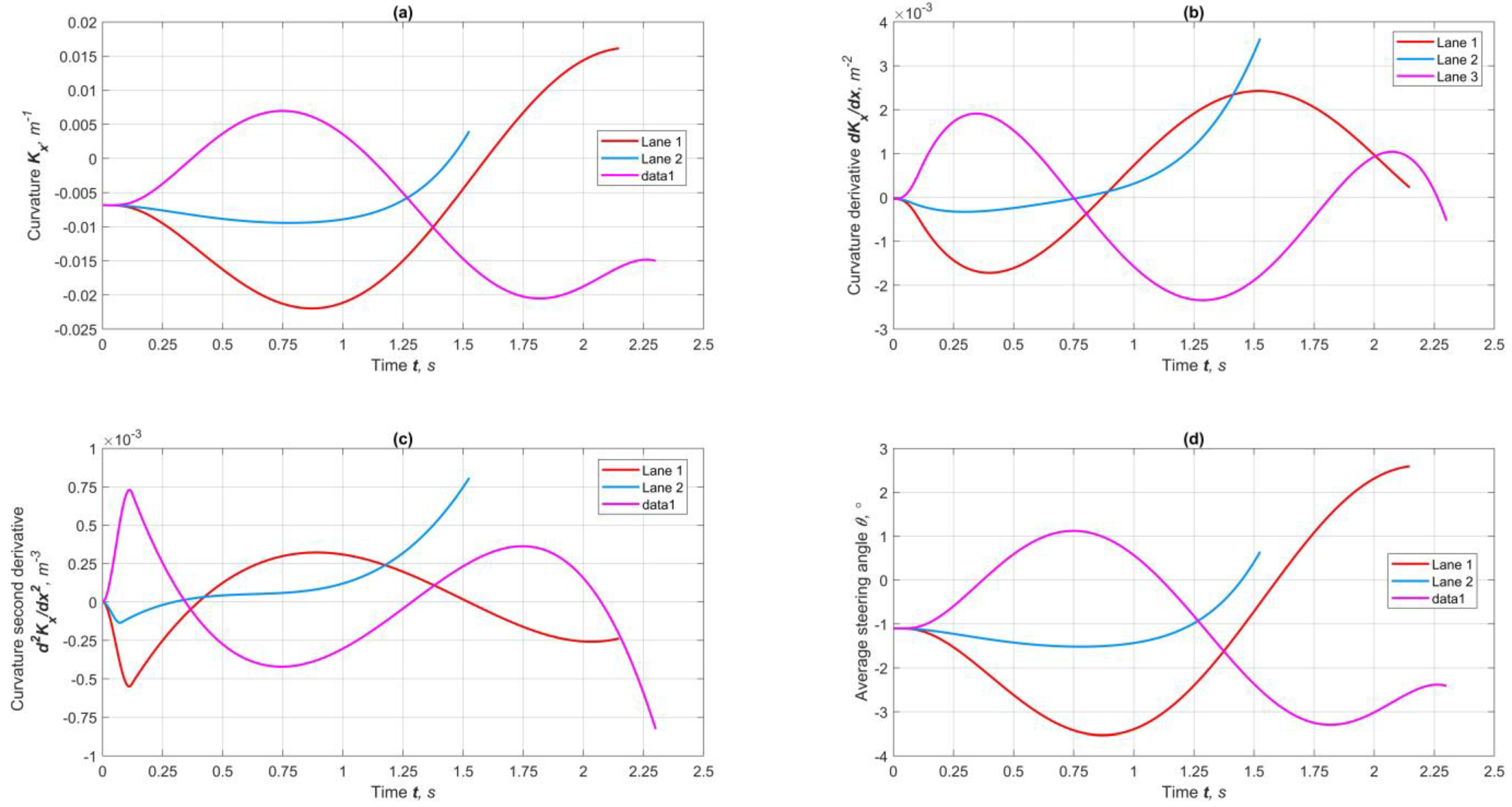
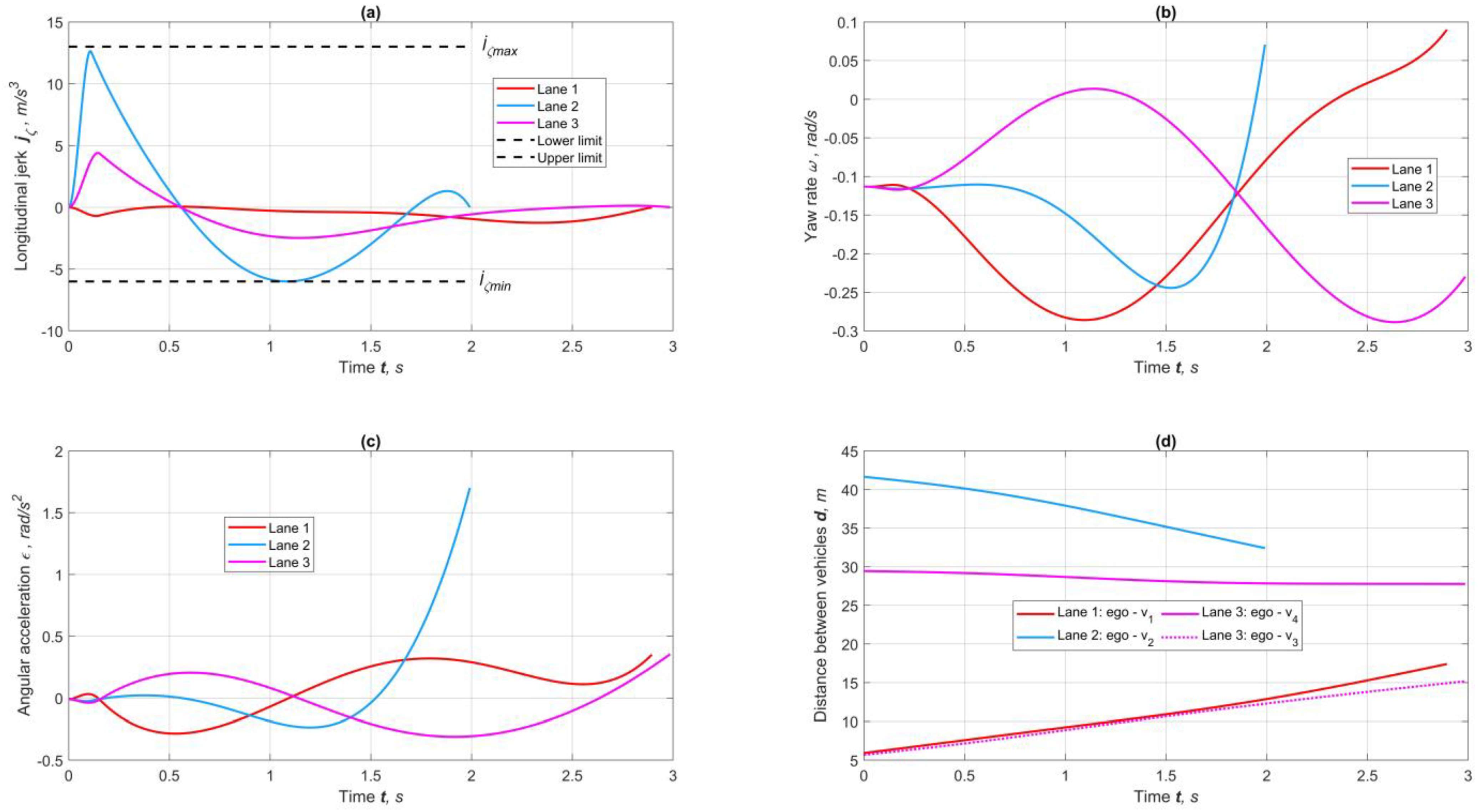
• Several key findings should be noted. First, because the method utilizes the derivatives of modeling parameters, followed by numerical integration, rather than simulating trajectories and speeds directly, it produces simple and smooth reference curves. All kinematic parameters, including jerks, ensure smoothness, clarity, and continuity between road segments. Second, the proposed technique requires a minimal number of varying parameters. While the cost function encompasses multiple optimization criteria, priority should be given to the accuracy of lateral displacement D and to ensuring motion safety in relation to other traffic participants. Finally, using nonlinear equality constraints, represented by integral numerical techniques, enhances prediction reliability compared with linear equality constraints, with minimal impact on optimization performance.
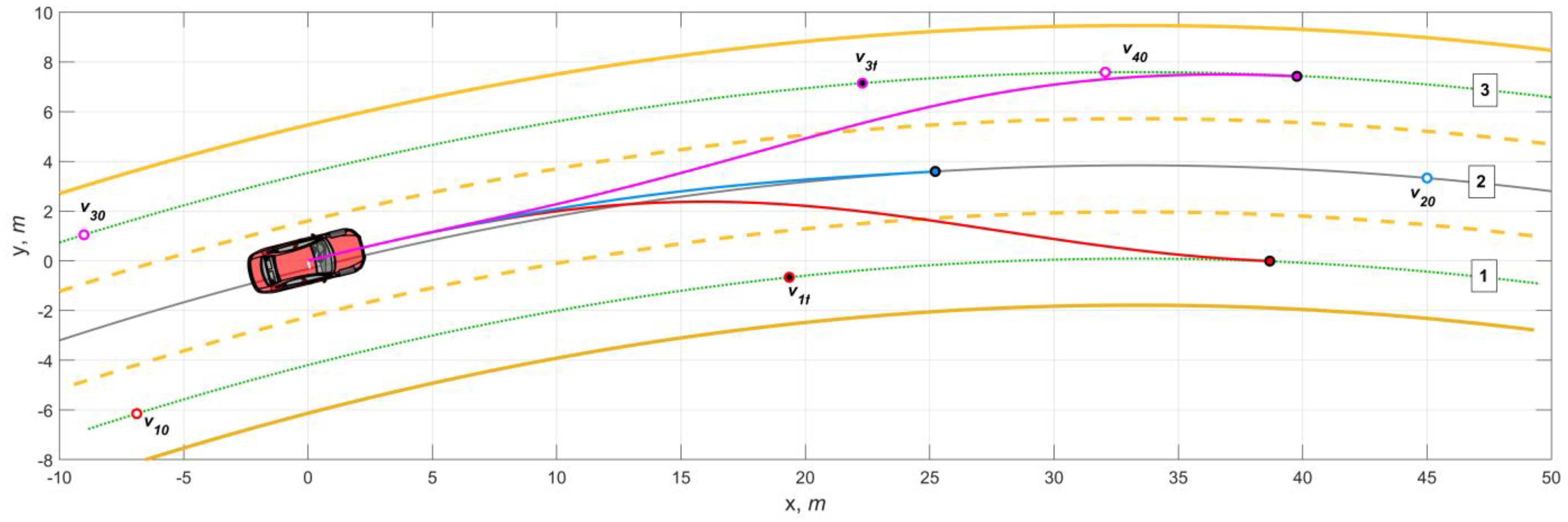
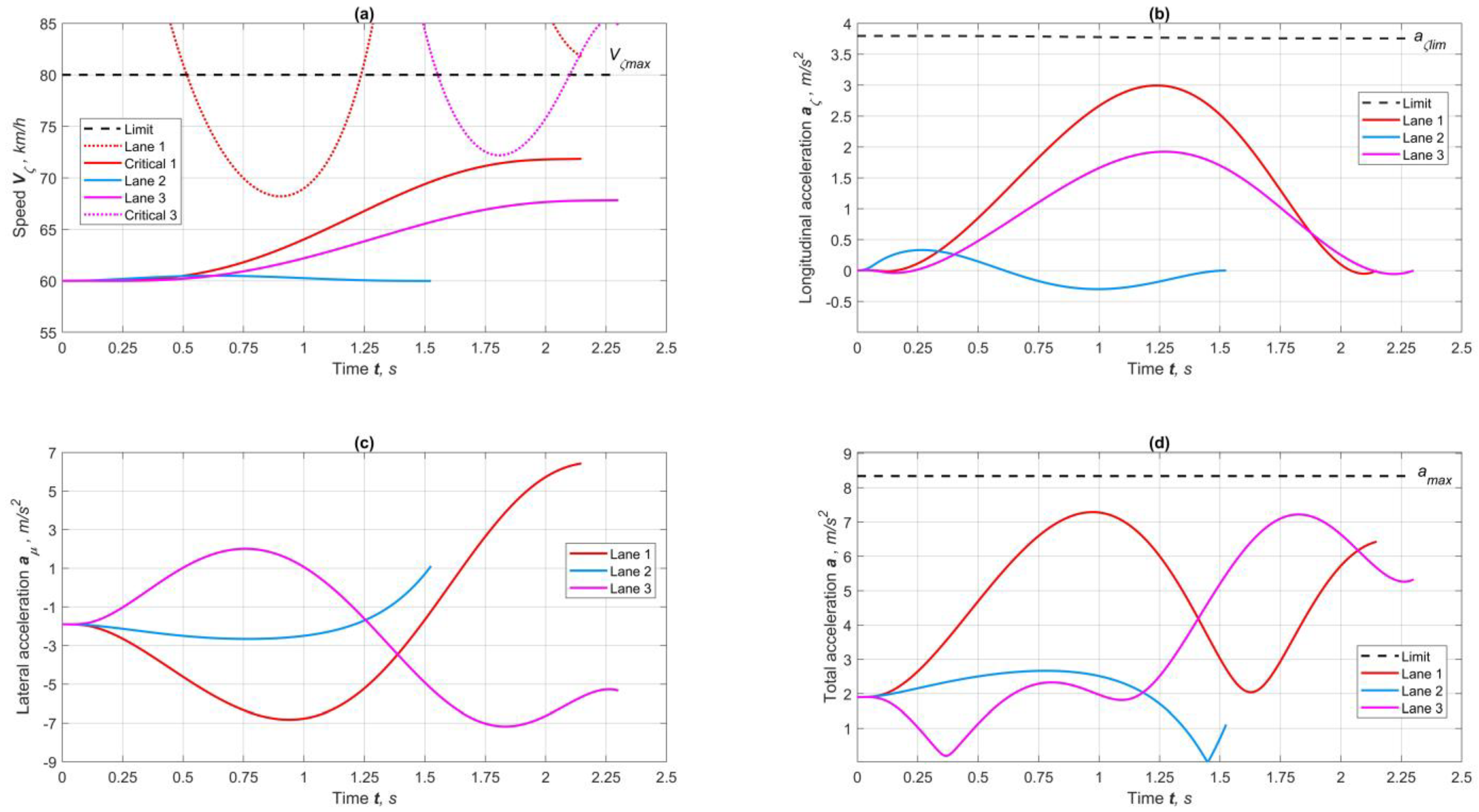
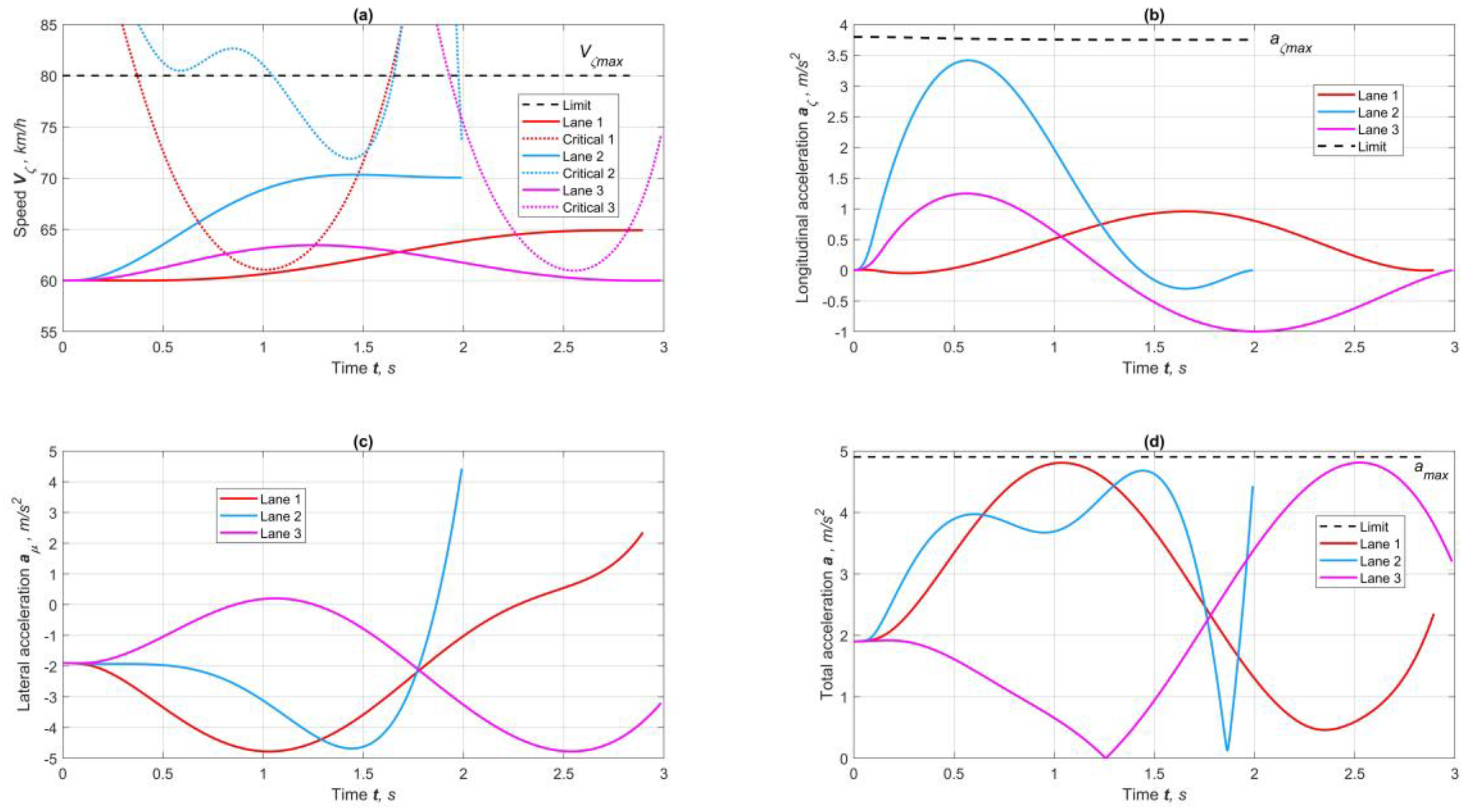
• The vehicle’s position and lane width were established prior to planning the motion, allowing for the generation of several trajectory variants with different lateral displacements (D). In this study, we focused on a minor deviation from the lane’s midline, resulting in the modeling of three maneuver variants. The criteria for selecting the best trajectory may include factors such as minimum transition time, maximum final speed, longest trajectory, minimum control cost, or a combination of these. However, this study did not address the selection of the most effective maneuver, as that topic is reserved for future research.
• All simulations were conducted on a laptop equipped with an 11th Gen Intel^® Core™ i7-1185G7 processor (Santa Clara, CA, USA) running at 3.00 GHz (base frequency: 1.80 GHz) and 16.0 GB of RAM, using a 64-bit version of Windows 10 Pro. The software environment utilized was MATLAB R2023b (The MathWorks, Natick, MA, USA), which provided the basic optimization function fmincon. On average, the computation time for one maneuver prognosis ranged from approximately 0.5 to 2.4 s, depending on the optimization settings, desired accuracy, and initial conditions.
• This study addresses a significant gap between theoretical models, such as action-based planners, and practical applications, making it applicable to both urban and highway AV systems. By bridging the integration gap between trajectory planning and speed management, the approach promotes more predictable, comfortable, and physically feasible autonomous motion. As AVs transition from controlled highway environments to complex urban settings, the proposed method—aligning dynamic constraints with real-time performance—is crucial in ensuring safe and passenger-friendly deployment. The inverse technique presented in this paper could establish a foundational tool for the next generation of motion planners.
• While this study advances motion planning with its inverse derivative-based approach, several limitations remain. The method assumes idealized conditions—perfect state estimation, all-wheel-drive dynamics, and simplified circular obstacles—which may degrade performance in real-world noisy environments or with heterogeneous vehicle platforms. Computational efficiency, though improved, could struggle with ultra-long horizons or dense urban scenarios, and the lack of hardware validation leaves open questions about real-world robustness. Future research should prioritize real-time enhancements (e.g., GPU acceleration), robust perception integration (e.g., sensor fusion for dynamic obstacle prediction), and experimental validation (e.g., on-road testing). Extending the framework to multi-agent coordination (e.g., V2X-enabled planning) could further broaden its impact. Addressing these gaps would bridge the divide between theoretical smoothness and deployable autonomy, making the method viable for safety-critical applications. Furthermore, future research should compare the proposed approach with other approaches in the literature using various criteria, including computation speed.

References

1. Xia, T.; Chen, H. A Survey of Autonomous Vehicle Behaviors: Trajectory Planning Algorithms, Sensed Collision Risks, and User Expectations. Sensors 2024, 24, 4808. [Google Scholar] [CrossRef]
2. Zhang, Y.; Chen, H.; Waslander, S.; Gong, J.; Xiong, G.; Yang, T.; Liu, K. Hybrid Trajectory Planning for Autonomous Driving in Highly Constrained Environments. IEEE Access 2018, 6, 32800–32819. [Google Scholar] [CrossRef]
3. Jiang, Y.; Jin, X.; Xiong, Y.; Liu, Z. A Dynamic Motion Planning Framework for Autonomous Driving in Urban Environments. In Proceedings of the 2020 39th Chinese Control Conference, Shenyang, China, 27–29 July 2020; pp. 5429–5435. [Google Scholar] [CrossRef]
4. Dang, D.; Gao, F.; Hu, Q. Motion Planning for Autonomous Vehicles Considering Longitudinal and Lateral Dynamics Coupling. Appl. Sci. 2020, 10, 3180. [Google Scholar] [CrossRef]
5. Li, G.; Zhang, X.; Guo, H.; Lenzo, B.; Guo, N. Real-Time Optimal Trajectory Planning for Autonomous Driving with Collision Avoidance Using Convex Optimization. Automot. Innov. 2023, 6, 481–491. [Google Scholar] [CrossRef]
6. Tang, X.; Li, B.; Du, H. A Study on Dynamic Motion Planning for Autonomous Vehicles Based on Nonlinear Vehicle Model. Sensors 2023, 23, 443. [Google Scholar] [CrossRef]
7. Liniger, A.; Gool, L. Safe Motion Planning for Autonomous Driving using an Adversarial Road Model. arXiv 2020. [Google Scholar] [CrossRef]
8. Yang, W.; Li, C.; Zhou, Y. A Path Planning Method for Autonomous Vehicles Based on Risk Assessment. World Electr. Veh. J. 2022, 13, 234. [Google Scholar] [CrossRef]
9. Hu, Z.; Yang, Z.; Liu, X.; Zhang, W. Radar-based path planning of autonomous surface vehicle with static and dynamic obstacles in a Frenet Frame. J. Navig. 2023, 76, 487–505. [Google Scholar] [CrossRef]
10. Jin, X.; Li, Z.; Ikiela, N.V.O.; He, X.; Wang, Z.; Tao, Y.; Lv, H. An Efficient Trajectory Planning Approach for Autonomous Ground Vehicles Using Improved Artificial Potential Field. Symmetry 2024, 16, 106. [Google Scholar] [CrossRef]
11. Dong, D.; Ye, H.; Luo, W.; Wen, J.; Huang, D. Collision Avoidance Path Planning and Tracking Control for Autonomous Vehicles Based on Model Predictive Control. Sensors 2024, 24, 5211. [Google Scholar] [CrossRef]
12. Jeng, S.-L.; Chieng, W.-H.; Wang, Y.-C. Real-Time Heuristic Motion Planning for Autonomous Vehicle Driving. J. Soc. Mech. Eng. 2021, 42, 187–196. [Google Scholar] [CrossRef]
13. Lu, Y.; He, S.; Li, Y.; Wu, Y.; Zhong, W. A real-time decoupling trajectory planning method for on-road autonomous driving. IET Control. Theory Appl. 2022, 17, 1800–1812. [Google Scholar] [CrossRef]
14. Cheng, J.; Chen, Y.; Zhang, Q.; Gan, L.; Liu, M. Real-Time Trajectory Planning for Autonomous Driving with Gaussian Process and Incremental Refinement. In Proceedings of the 2022 International Conference on Robotics and Automation (ICRA), Philadelphia, PA, USA, 23–27 May 2022; pp. 8999–9005. [Google Scholar]
15. Jiang, Y.; Liu, Z.; Qian, D.; Zuo, H.; He, W.; Wang, J. Robust Online Path Planning for Autonomous Vehicle Using Sequential Quadratic Programming. In Proceedings of the IEEE Intelligent Vehicles Symposium (IV), Aachen, Germany, 5–9 June 2022; pp. 175–182. [Google Scholar] [CrossRef]
16. Li, B.; Ouyang, Y.; Li, L.; Zhang, Y. Autonomous Driving on Curvy Roads Without Reliance on Frenet Frame: A Cartesian-Based Trajectory Planning Method. IEEE Trans. Intell. Transp. Syst. 2022, 23, 15729–15741. [Google Scholar] [CrossRef]
17. Scheffe, P.; Henneken, T.M.; Kloock, M.; Alrifaee, B. Sequential Convex Programming Methods for Real-Time Optimal Trajectory Planning in Autonomous Vehicle Racing. IEEE Trans. Intell. Veh. 2022, 8, 661–672. [Google Scholar] [CrossRef]
18. Diachuk, M.; Easa, S.M. Path and control planning for autonomous vehicles in restricted space and low speed. J. Infrastruct. 2020, 5, 42. [Google Scholar] [CrossRef]
19. Pérez-Dattari, R.; Brito, B.; de Groot, O.; Kober, J.; Alonso-Mora, J. Visually-guided motion planning for autonomous driving from interactive demonstrations. Eng. Appl. Artif. Intell. 2022, 116, 105277. [Google Scholar] [CrossRef]
20. Diachuk, M.; Easa, S.M. Improved mathematical approach for modeling sport differential mechanism. Vehicles 2022, 4, 1122–1157. [Google Scholar] [CrossRef]
21. Diachuk, M.; Easa, S.M. Modeling combined operation of engine and torque converter for improved vehicle powertrain’s complex. Vehicles 2022, 4, 433–444. [Google Scholar] [CrossRef]
22. Diachuk, M.; Easa, S.M. Improved models of vehicle differential mechanisms using various approaches. Int. J. Veh. Syst. Model. Test. 2023, 17, 210–230. [Google Scholar] [CrossRef]
23. Diachuk, M.; Easa, S.M. Motion planning for autonomous vehicles using sequential optimization. Vehicles 2022, 4, 808–824. [Google Scholar] [CrossRef]
24. Diachuk, M.; Easa, S.M. Using inverse dynamics technique in planning autonomous vehicle speed mode considering physical constraints. Highlights Veh. 2023, 1, 29–53. [Google Scholar] [CrossRef]
25. Dorpmüller, P.; Schmitz, T.; Bejagam, N.; Bertram, T. Time-Optimal Trajectory Planning in Highway Scenarios Using Basis-Spline Parameterization. In Proceedings of the IEEE 26th International Conference on Intelligent Transportation Systems (ITSC), Bilbao, Spain, 24–28 September 2023; pp. 596–601. [Google Scholar] [CrossRef]
26. Wang, Y.; Lin, Z. Research on path planning for autonomous vehicle based on Frenet system. J. Eng. Res. 2023, 11, 100080. [Google Scholar] [CrossRef]
27. Trauth, R.; Moller, K.; Würsching, G.; Betz, J. FRENETIX: A High-Performance and Modular Motion Planning Framework for Autonomous Driving. IEEE Access 2024, 12, 127426–127439. [Google Scholar] [CrossRef]
28. Huang, H.; Liu, Y.; Liu, J.; Yang, Q.; Wang, J.; Abbink, D.; Zgonnikov, A. General Optimal Trajectory Planning: Enabling Autonomous Vehicles with the Principle of Least Action. Engineering 2023, 33, 63–76. [Google Scholar] [CrossRef]
29. Diachuk, M.; Easa, S.M. Planning speed mode of all-wheel drive autonomous vehicles considering complete constraint set. Vehicles 2024, 6, 191–230. [Google Scholar] [CrossRef]
30. Diachuk, M.; Easa, S.M. Simultaneous trajectory and speed planning for autonomous vehicles considering maneuver variants. Appl. Sci. 2024, 14, 1579. [Google Scholar] [CrossRef]
31. MATLAB R2022b. 2023. Available online: https://www.mathworks.com/ (accessed on 22 January 2023).
32. Audi A4 Quatro Characteristics. 2023. Available online: http://www.automobile-catalog.com/car/2011/1187660/audi_a4_3_2_fsi_quattro_attraction_tiptronic.html (accessed on 19 January 2023).
Figure 1. Study methodology.
Wevj 16 00272 g001
Figure 2. Scheme of the ideal vehicle kinematics model.
Wevj 16 00272 g002
Figure 3. Basic geometric parameters: (a) Scheme of forming AV trajectory using Frenet coordinates. (b) Trajectory variants and distances to moving obstacles.
Wevj 16 00272 g003
Figure 4. Scheme of numerical integration at specified points.
Wevj 16 00272 g004
Figure 5. Prediction of lane-change trajectories with friction factor φmax = 0.85.
Wevj 16 00272 g005
Figure 6. Results of forecasting speeds and accelerations for maneuvers at friction factor φmax = 0.85: (a) longitudinal and critical (sideslip) speeds, (b) longitudinal accelerations, (c) lateral accelerations, and (d) total accelerations.
Wevj 16 00272 g006
Figure 7. Results of forecasting kinematic parameters of maneuvers at φmax = 0.85: (a) longitudinal jerk, (b) yaw rate, (c) angular acceleration, and (d) distance to obstacles.
Wevj 16 00272 g007
Figure 8. Results of geometric indicators for forecasting lane maneuvers at φmax = 0.85: (a) curvature, (b) curvature’s first derivative, (c) curvature’s second derivative, and (d) steering angle.
Wevj 16 00272 g008
Figure 9. Prediction of lane-change trajectories under the condition φmax = 0.5.
Wevj 16 00272 g009
Figure 10. Results of forecasting speeds and accelerations for maneuvers at friction factor φmax = 0.5: (a) longitudinal and critical (sideslip) speeds, (b) longitudinal accelerations, (c) lateral accelerations, and (d) total accelerations.
Wevj 16 00272 g010
Figure 11. Results of forecasting kinematic parameters of maneuvers at φmax = 0.5: (a) longitudinal jerk, (b) yaw rate, (c) angular acceleration, and (d) distance to obstacles.
Wevj 16 00272 g011
Figure 12. Results of geometric indicators for forecasting lane maneuvers at φmax = 0.5: (a) curvature, (b) curvature’s first derivative, (c) curvature’s second derivative, (d) steering angle.
Wevj 16 00272 g012