Trajectory Optimization for Autonomous Highway Driving Using Quintic Splines

Abstract

This paper introduces a robust and efficient Localized Spline-based Path-Planning (LSPP) algorithm designed to enhance autonomous vehicle navigation on highways. The LSPP approach prioritizes smooth maneuvering, obstacle avoidance, passenger comfort, and adherence to road constraints, including lane boundaries, through optimized trajectory generation using quintic spline functions and a dynamic speed profile. Leveraging real-time data from the vehicle’s sensor fusion module, the LSPP algorithm accurately interprets the positions of surrounding vehicles and obstacles, creating a safe, dynamically feasible path that is relayed to the Model Predictive Control (MPC) track-following module for precise execution. The theoretical distinction of LSPP lies in its modular integration of: (1) a finite state machine (FSM)-based decision-making layer that selects maneuver-specific goal states (e.g., keep lane, change lane left/right); (2) quintic spline optimization to generate smooth, jerk-minimized, and kinematically consistent trajectories; (3) a multi-objective cost evaluation framework that ranks competing paths according to safety, comfort, and efficiency; and (4) a closed-loop MPC controller to ensure real-time trajectory execution with robustness. Extensive simulations conducted in diverse highway scenarios and traffic conditions demonstrate LSPP’s effectiveness in delivering smooth, safe, and computationally efficient trajectories. Results show consistent improvements in lane-keeping accuracy, collision avoidance, enhanced materials wear performance, and planning responsiveness compared to traditional path-planning methods. These findings confirm LSPP’s potential as a practical and high-performance solution for autonomous highway driving.

1. Introduction

With the rapid advancement of intelligent transportation systems [1] and automobile technology [2], fully automated vehicles have garnered significant attention from researchers due to their diverse potential applications [3]. According to a 2024 McKinsey report, the global autonomous vehicle market is projected to reach USD 620 billion by 2030, reflecting increased investment in autonomous mobility solutions. These vehicles integrate multidisciplinary knowledge and theories, with perception [4], decision [5], and control [6] being the three main components of their software configuration. Central to the decision and control aspects are the path-planning and path-tracking problems [7]. Self-driving cars necessitate fast and reliable path planning and road boundary following functionalities that ensure safety (recent data from the U.S. Department of Transportation show that lane departure and collision avoidance technologies could reduce roadway fatalities by up to 37%), provide comfortable rides [8], maintain vehicle control in extreme conditions, and remain highly effective at high speeds [9]. A 2023 survey by the World Economic Forum indicates that over 60% of global automotive OEMs are prioritizing the integration of Level 4 autonomy in highway driving as part of their near-term development roadmap.

In autonomous driving, both path and motion planning are essential components, ensuring a vehicle can navigate safely and efficiently. Path planning involves determining a feasible route from the current position to a desired destination, taking into account obstacles, traffic rules, and road geometry. This high-level planning ensures that the vehicle follows a safe and efficient path. Motion planning, on the other hand, focuses on the precise control needed to follow the planned path. It involves generating detailed trajectories that account for the vehicle’s dynamics and kinematics, ensuring smooth and safe movement in real-time conditions.

While path planning sets the strategic route, motion planning handles the tactical execution, dealing with immediate obstacles and ensuring the vehicle’s movements are safe and comfortable. This paper focuses specifically on motion planning, addressing the critical aspects of generating and following detailed trajectories to ensure precise and safe vehicle operation in various driving scenarios. Specifically, it examines motion planning for highways, highlighting the challenges and solutions for navigating these complex settings efficiently and safely.

Motion planning involves a sequence of steps that consider the state of the egocar (such as speed, orientation, and global reference position), its surrounding environment (including moving vehicles, static obstacles, and drivable spaces), traffic regulations, and potential maneuvers [10]. This process generates a safe, optimized, collision-free trajectory and a speed profile that the autonomous car must follow.

1.1. Components of the Path Planning

The path planner of autonomous cars consists of several sequential tasks or modules, each contributing to generating a safe and efficient route from the current position to the desired destination. Here are the key tasks or modules involved:

• Perception and Environment Mapping:

  -

  Sensor Data Acquisition: Collect data from sensors like LiDAR, radar, cameras, and GPS [11].

  -

  Object Detection and Tracking: Identify and track surrounding vehicles [12], pedestrians [13], and other obstacles [14].

  -

  Environment Mapping: Create a detailed map of the surroundings, including static and dynamic objects.

• Localization:

  -

  Position Estimation: Determine the precise location of the egocar using GPS, IMU, and sensor data [15].

  -

  Map Matching: Align the vehicle’s estimated position with a high-definition map for accurate localization [16].

• Route Planning:

  -

  Global Path Planning: Determine a high-level route from the current location to the destination, considering road networks and traffic regulations [17].

  -

  Waypoints Generation: Create intermediate waypoints along the global path to guide the vehicle.

• Behavior Planning:

  -

  Scenario Analysis: Evaluate possible driving scenarios, such as lane changes, merges, and turns [5].

  -

  Decision Making: Choose the optimal driving behavior based on traffic rules, road conditions, and surrounding vehicles [18].

• Path Generation:

  -

  Feasibility Check: Ensure the planned path is drivable and avoids obstacles [19].

  -

  Path Smoothing: Generate a smooth and continuous path using techniques like splines or polynomial curves [20].

• Trajectory Planning:

  -

  Trajectory Optimization: Create a detailed, time-parameterized trajectory that specifies the vehicle’s position, velocity, and acceleration.

  -

  Collision Avoidance: Adjust the trajectory to avoid potential collisions with dynamic and static obstacles [21].

• Speed Profile Generation:

  -

  Speed Planning: Determine an optimal speed profile along the planned path, considering speed limits, curvature, and traffic conditions [21].

  -

  Comfort and Safety Considerations: Ensure the speed profile provides a comfortable ride and adheres to safety constraints [22].

• Control Interface:

  -

  Command Generation: Convert the planned trajectory and speed profile into control commands for the vehicle’s actuators (steering, throttle, brake) [18].

  -

  Feedback Loop: Continuously monitor the vehicle’s execution and adjust the commands as needed to stay on the planned path [19].

These modules work together in a continuous loop, constantly updating the vehicle’s plan based on new sensor data and changes in the environment to ensure safe and efficient navigation [23]. The 4th to 8th tasks/modules from the above list are considered representative of motion planning, which is the main focus in this paper. These tasks collectively handle the detailed execution of the high-level path, ensuring the vehicle moves smoothly, safely, and efficiently according to real-time conditions and vehicle dynamics.

1.2. Background and Literature Review

Currently, several approaches for generating a motion path are reported in the literature. These can be classified into the following categories:

1.2.1. Space Configuration

The main idea of this approach is to build an occupancy grid map, where the current state of the ego-car and the relative positions of surrounding obstacles significantly influence the map’s construction. The space around the egocar is divided into rectangular or square cells, each evaluated for occupancy. Non-occupied cells are considered collision-free and tagged as potential spaces for the ego car’s next maneuver. These collision-free cells are then connected to form potential trajectories for the ego car. Several algorithms, such as Voronoi diagrams [24], lattices, and sampling-based methods, are used to evaluate and connect non-occupied cells. These algorithms are relatively fast; however, they do not guarantee that the generated solutions are suitable from a dynamics perspective. In other words, the outcomes of these algorithms often do not consider the dynamic model of the car and its degrees of freedom, making many of the solutions infeasible.

1.2.2. Path-Finders

These techniques aim to find the feasible and optimal path between point A and point B on a map or graph. “Optimal” here means optimized according to one or more cost functions, such as the shortest distance or lowest travel time. The state-of-the-art path-finding algorithms include A*, Dijkstra, and rapidly exploring random tree (RRT) algorithms [25]. Both A* and Dijkstra require prior knowledge of the environment, while RRT-based algorithms do not. However, similar to space configuration algorithms, these path-finding algorithms can sometimes produce trajectories that are not feasible for vehicles, as they do not account for vehicle dynamics.

1.2.3. Attractive and Repulsive Fields

These algorithms create artificial forces (fields) that update the car’s current state and guide it toward the desired target position while avoiding obstacles. Attractive forces pull the car toward the goal position, while repulsive forces push it away from obstacles’ positions. The resultant force acting on the car is the sum of the attractive and repulsive forces. The car’s position is updated by moving it in the direction of the resultant force [26]. The main drawbacks of these algorithms are their tendency to get stuck in local minima while searching for feasible solutions and their potential to produce unstable solutions for self-driving cars.

1.2.4. Curves

The techniques in this category generate local paths as curves that can be expressed using algebraic or mathematical functions [27], such as splines, clothoids, and Bezier curves [28]. These curves are created based on the status of the ego car and the road ahead. There are two primary implementation methods within this category: (a) Point-Free Method: Curves represent feasible trajectories that respect the car’s kinematic and dynamic constraints, allowing for legal maneuvers. (b) Point-to-Point Method: Curves are used to define a trajectory between two waypoints. The main drawback of these algorithms is that each generated curve, which could be a potential trajectory for the ego car, must be evaluated for kinematic and dynamic feasibility and collision avoidance. Practical implementation and real-time execution of these algorithms can be computationally intensive, placing a high load on the CPU.

1.2.5. Artificial Intelligence Schemes

This category of algorithms incorporates human-like perception, cognition, and reasoning to solve engineering problems. For local path planning, techniques such as fuzzy logic, neural networks [29], particle swarm optimization, genetic algorithms, ant colony optimization, bacterial foraging optimization, artificial bee colony, cuckoo search, and shuffled frog leaping algorithms are commonly used. These methods effectively handle uncertainties in problem formulation and solution spaces, eliminating the need for precise mathematical models for design and parameter tuning. Detailed insights into artificial intelligence techniques applied to local path planning for autonomous cars can be found in [18]. However, the main drawbacks of these algorithms are their complexity and the high computational demands for real-time execution, often requiring substantial CPU or GPU resources.

Combining the aforementioned techniques is also a common approach to overcome their individual limitations [20]. For instance, curve-based methods are often integrated with numerical optimization solvers to generate practical trajectories that respect vehicle dynamics while optimizing for objectives such as minimal travel distance [28], shortest travel time, energy efficiency, and maximum comfort [30]. Similarly, the Artificial Potential Field (APF) algorithm can be combined with Model Predictive Control (MPC) to enhance the feasibility and performance of generated trajectories [31]. However, as more algorithms are combined, the complexity and computational demands increase, making real-time execution more challenging.

1.2.6. Research Gap

Synthesizing the limitations discussed above, existing motion planning approaches often face a critical trade-off. Methods prioritizing computational speed (e.g., grid-based, basic RRT) frequently produce paths that are kinematically infeasible or lack the smoothness required for passenger comfort, especially at high speeds (drawbacks from Section 1.2.1 and Section 1.2.2). Conversely, techniques focusing on optimality or smoothness (e.g., complex optimization, AI, some spline methods) can become computationally prohibitive for real-time applications or struggle with dynamic obstacle avoidance (drawbacks from Section 1.2.4 and Section 1.2.5). Furthermore, ensuring seamless integration between high-level decision-making (behavior planning) and low-level, dynamically consistent trajectory generation remains a significant challenge [Ref Gap Statement idea]. Specifically, there is a need for a method that simultaneously achieves:

-

High-order Smoothness: Guaranteeing continuity up to the jerk level (C3 continuity) for enhanced comfort and stability, often neglected by methods using lower-order polynomials or discrete path segments.

-

Real-time Performance: Maintaining low computational latency suitable for dynamic highway environments.

-

Kinematic Feasibility: Directly generating trajectories that respect vehicle dynamic constraints.

-

Integrated Decision and Planning: Cohesively linking behavioral decisions (like lane changes) with the generation of smooth, executable trajectories.

This paper presented the Localized Spline-based Path Planning (LSPP) algorithm, designed to address key limitations of existing methods, namely the trade-offs between trajectory smoothness, computational efficiency, and kinematic feasibility in dynamic highway environments. By uniquely integrating an FSM, localized quintic splines ensuring jerk continuity, and MPC tracking, LSPP is able to balance smoothness with real-time responsiveness effectively, making it a robust solution for both structured and semi-structured driving environments. The main contributions and innovations of this work are:

• A Novel Integrated Framework: We propose a tightly integrated architecture combining a rule-based Finite State Machine (FSM) for maneuver selection, localized quintic spline generation for C3-continuous path segments, and Model Predictive Control (MPC) for robust tracking. This addresses the integration challenge often present in modular approaches.
• Jerk-Minimized Highway Trajectories: We specifically leverage quintic splines to ensure jerk continuity, directly addressing the need for high passenger comfort and vehicle stability during high-speed highway driving, a limitation in methods offering only curvature continuity or less smooth paths.
• Computationally Efficient Localized Planning: The use of localized spline generation, triggered by the FSM and updated based on real-time sensor data, provides adaptability to dynamic environments while maintaining computational efficiency compared to global optimization or exhaustive search methods.
• Systematic Comparative Evaluation: We provide a quantitative comparison against standard benchmarks (A*, RRT, Bezier Curves) across multiple representative highway scenarios, demonstrating LSPP’s superior performance in terms of smoothness, safety metrics, and execution speed.

While the foundational components utilized in LSPP—namely, Finite State Machines, spline-based curve fitting, and Model Predictive Control—are established concepts in robotics and control, the novelty of this work lies in their specific synergistic integration and tailored design within the proposed LSPP architecture (Figure 1). LSPP distinguishes itself by:

-

Employing a custom-designed FSM (detailed in Section 2.2.1, Tables 1–3), incorporating nuanced cost functions specifically for optimizing highway driving maneuvers like lane changes and overtaking.

-

Leveraging localized quintic spline generation (Section 2.1.2 and Section 2.2.4) triggered by the FSM. This ensures jerk continuity (C3 smoothness), critical for high-speed passenger comfort and vehicle stability, a higher standard than typically achieved with cubic or Bezier alternatives.

-

Tightly coupling the spline generator with the MPC tracker (Section 2.2.2) enables high-fidelity execution of these smooth, dynamically adapted trajectories while respecting vehicle kinematic limits (Equation (2)). This purpose-built integration results in a motion planner that effectively balances high-order smoothness, real-time responsiveness, and computational efficiency specifically for structured highway environments, addressing the trade-offs often found in existing approaches.

2. Methods

2.1. Foundation of Motion Planning

The following sections shed light on the foundation of the proposed motion planner:

2.1.1. Path Planning Architecture

Figure 1 represents a comprehensive architecture of a path planning and control system for an autonomous vehicle, showcasing the flow of information between various modules and components that contribute to trajectory planning and vehicle control.

The system initiates with the mission planner module (MPM), which is supplied with inputs from both the GPS and a global digital street map. These inputs enable the MPM to generate a high-level trip route. This route is then forwarded to the Rule-Based Localized Path Planner (RBLPP), which uses this information to extract a nearby segment of the route (according to the current ego car coordinates) and generate for this segment approximate waypoints, defining the start, end, and some midpoint positions for it. The RBLPP also receives critical information on moving and stationary local objects from the Object Detection Module (ODM), which integrates data from multiple sensors, including cameras, radars, lidars, and sensor fusion algorithms [12,13,14,15]. Each of these sensors feeds its data into the sensor fusion module, which processes and combines the data to form a coherent understanding of the vehicle’s surrounding environment.

The approximate waypoints generated by the RBLPP are subsequently refined by the Spline-Trajectories Generator, which produces more accurate trajectories for the vehicle to follow. These refined trajectories are then supplied to the MPC (Model Predictive Control) Controller, which is responsible for generating the necessary control commands to actuate the vehicle. The MPC outputs steering commands and throttle/brake commands, which are sent to the vehicle’s actuators, ensuring precise and responsive control of the egocar.

The modules within the green oval in Figure 1 represent the motion planner, which is the main focus of this paper, which determines what behavior the vehicle should exhibit at any point in time (e.g., stopping at a traffic light or intersection, changing lanes, accelerating, or making a left turn onto a new street, etc.).

2.1.2. Key Characteristics of Quintic Polynomials

A quintic spline polynomial is a piecewise-defined polynomial function used in interpolation and approximation of data to create smooth curves that pass through or near a set of data points. They are characterized as follows:

• Piecewise Definition: A spline is defined by multiple polynomial segments, each valid over a specific interval. For example, a quintic spline is composed of 5th-order polynomials defined piecewise between each pair of waypoints $\left(x_i, y_i\right) and \left(x_{i+1}, y_{i+1}\right)$:

  $$\begin{array}{l}{y}_i\left(x\right)=a_i+b_i\left(x-x_i\right)+c_i{\left(x-x_i\right)}^2+d_i{\left(x-x_i\right)}^3+e_i{\left(x-x_i\right)}^4+f_i{\left(x-x_i\right)}^5\\ for x\in \left[x_i, x_{i+1}\right]\end{array}$$

  (1)
• The choice of quintic (5th order) polynomials is specifically motivated by the need to define a trajectory segment by specifying not only position and velocity but also acceleration at both the start and end points. This requires six boundary conditions per spatial dimension (e.g., x(0), ẋ(0), ẍ(0), x(T), ẋ(T), ẍ(T)), which perfectly matches the six coefficients available in a quintic polynomial (Equation (1)). This capability is essential for generating dynamically smooth and feasible paths for vehicles.
• Continuity and Smoothness: Splines are constructed to ensure a certain level of smoothness at the points where the polynomial pieces join (called knots). For quintic splines, the first, second, third, and fifth derivatives are usually continuous across the intervals, making the transition between segments very smooth.
• Local Control: Each segment of the spline is influenced mainly by its local data points (waypoints received from the RBLPP), allowing for localized changes in the shape of the curve without significantly affecting the entire curve.
• Boundary Conditions: When constructing splines, additional conditions are needed at the endpoints to uniquely determine the spline. Common boundary conditions include specifying the values of derivatives up to the 4th order at the endpoints, and higher order derivatives are set to zero.

For $n+1$ data points $\left(x_0, y_0\right), \left(x_0, y_0\right), \dots , \left(x_n, y_n\right)$, a quintic spline $S_n$ consists of n quintic polynomials given by Equation (1), defined on each interval $\left[x_i, x_{i+1}\right]$. The coefficients $a_i, b_i, c_{i }, d_i, e_i, and f_i$ are determined by solving a system of equations that enforce: (1) The spline passing through or very close to the data points. (2) Continuity of the spline and its first, second, third, and fourth derivatives at each knot. (3) The chosen boundary conditions.

2.1.3. The Proposed Motion Planner

Behavior planning involves three key components: (1) predicting the behavior of obstacles, including other vehicles on the road, (2) making high-level decisions on the appropriate actions to achieve the desired goal safely and efficiently, such as slowing down, accelerating, turning, or changing lanes, and (3) generating trajectories that translate these decisions into a feasible path, typically represented as a series of waypoints or a mathematical formula, for the vehicle’s control system to execute [32].

The proposed LSPP protocol operates as follows:

• Interpolate waypoints for a nearby section (30 to 50 m long) of the route provided by the MPM.
• Determine the state of the egocar, including its position, orientation, velocity, and acceleration.
• Generate a set of predicted trajectories for each surrounding vehicle using data received from the ODM.
• Identify the available states for the egocar, such as “keep lane,” “change lanes to the right,” or “change lanes to the left.”
• For each available state, generate a target end state for the egocar and create multiple randomized potential trajectories by slightly perturbing elements of the target state. These “Jerk-Minimized Trajectories” (JMTs) [33] are quintic spline polynomials derived from the current initial and desired final values of position, velocity, and acceleration [34].
• Evaluate each potential trajectory using a set of cost functions that reward efficiency and penalize factors such as collisions, excessive jerks, or exceeding speed limits.
• Select the trajectory with the lowest cost.
• Assess this trajectory at the next several 20-millisecond intervals (the rate at which the data is received from the sensor fusion module) [35].
• Append these evaluations to the retained portion of the previous path.
• Send the updated path to the MPC controller for execution.

The Jerk Minimizing Trajectory (JMT) algorithm is implemented in C++ [36] to generate smooth trajectories that minimize sudden changes in acceleration, resulting in more comfortable and safer driving.

The JMT calculation involves finding the coefficients of a polynomial (5th order in quintic spline) that describes the vehicle’s path from a given start state to an end state over a specified time T (usually indicating the required speed profile). The key components of the algorithm can be portrayed as follows:

• Input Parameters:

  -

  Start: A vector of three elements [position, velocity, acceleration] representing the initial state of the vehicle.

  -

  End: A vector of three elements [position, velocity, acceleration] representing the final state of the vehicle.

  -

  T: The time duration over which the vehicle should move from the start state to the end state.

• Output:

  -

  A vector of coefficients for a 5th-degree polynomial of the form: $p\left(t\right)=a_0+a_{1}t+a_2{t}^2+a_3{t}^3+a_4{t}^4+a_5{t}^5$.

  -

  These coefficients are determined to minimize jerk over the time T.

• Calculation:

  -

  A system of equations is set up using the boundary conditions provided by the start and end states.

The C++ Eigen library [36] is used to solve this system and find the polynomial coefficients.

2.2. Implementation of the LSPP

The implementation of the LSPP algorithm hinges on the carefully orchestrated interaction between its core components. While based on known principles, their specific configuration and interplay, as detailed below, form the basis of LSPP’s effectiveness for highway navigation.

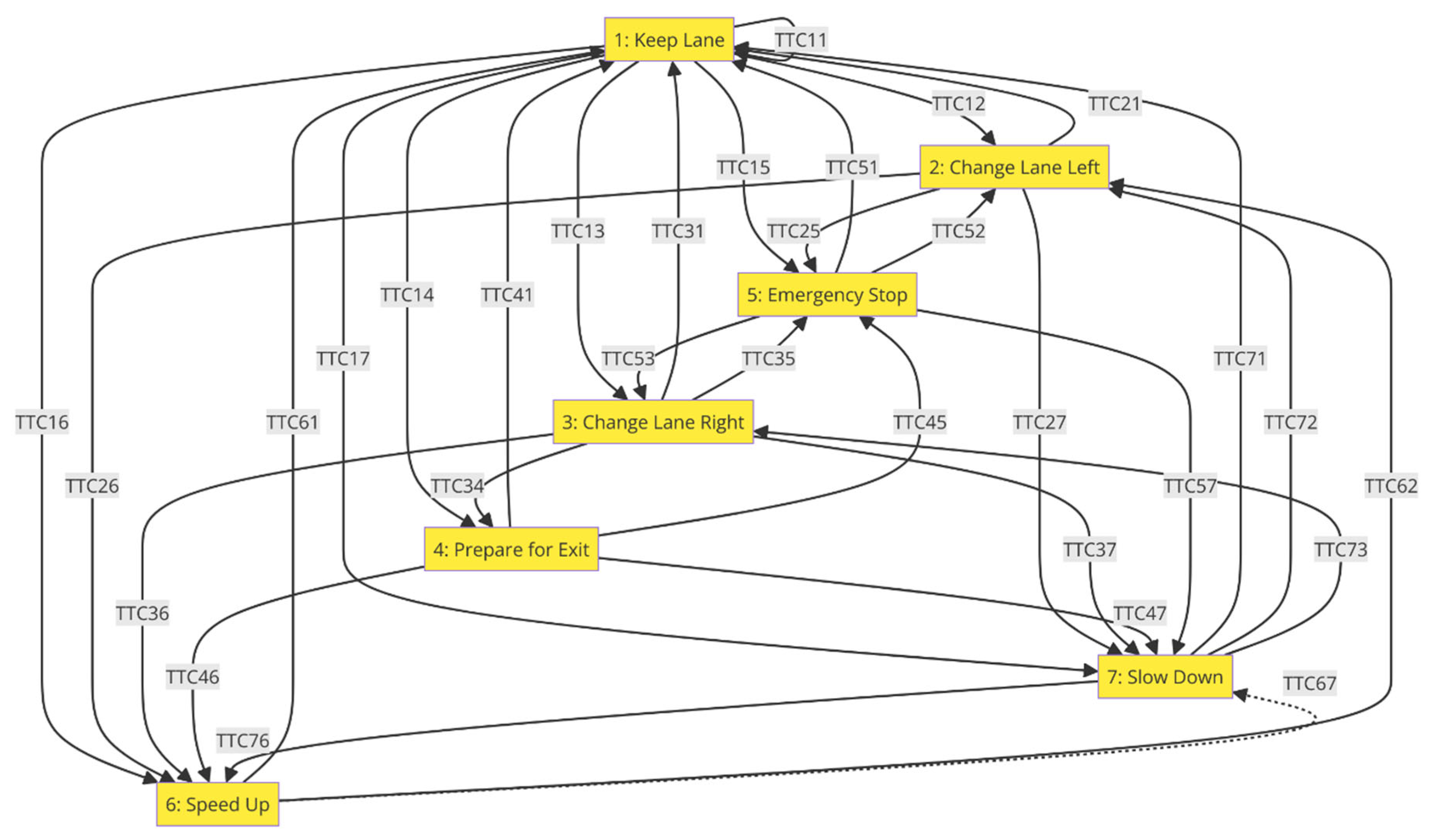
2.2.1. The Finite State Machine

While driving on the highway, the egocar typically considers several key driving states. These states help the car adapt its behavior based on the surrounding environment, including the positions of other vehicles and obstacles. In the design of the proposed LSPP algorithm, the states that the egocar can occupy are listed in

Table 1. Key driving states.

#	Ego Car State	Description	Possible Transitions	Triggering Conditions	Relevant Cost Functions
1	Keep Lane	The ego car stays in its current lane, maintaining a safe distance from vehicles.	- Change Lane Left - Change Lane Right - Emergency Stop - Speed Up - Slow Down - Keep Lane	- Safe distance maintained - No vehicles blocking the lane - Speed close to target	- Speed cost (maintain target speed) - Collision cost (avoid rear-end collisions) - Lane preference cost
2	Change Lane Left	The ego car shifts to the left lane, typically to overtake a slower vehicle.	- Keep Lane - Emergency Stop	- The left lane is clear - The left lane offers higher speed efficiency - Safe to maneuver	- Collision cost (check for vehicles in the left lane) - Jerk cost (minimize jerk) - Overtaking efficiency cost
3	Change Lane Right	The ego car shifts to the right lane, typically to make way for faster traffic.	- Keep Lane - Emergency Stop	- The right lane is clear - Need to avoid slower or obstructed vehicles - Approaching an exit	- Collision cost (check for vehicles in the right lane) - Lane preference cost - Jerk cost (minimize jerk)
4	Prepare for Exit	The ego car prepares to leave the highway by moving into the exit lane.	- Take Exit - Change Lane Right - Emergency Stop	- Exit approaching within a certain distance - The right lane is clear to merge into an exit lane	- Lane preference cost (moving toward the exit) - Speed cost (maintain appropriate speed for exit) - Fuel Efficiency cost
5	Emergency Stop	The ego car decelerates rapidly to avoid a collision or stop for an obstacle.	- Keep Lane - Change Lane Left/Right (if possible)	- Obstacle detected ahead - Collision is imminent - Severe traffic jam	- Collision cost (avoidance) - Jerk cost (smooth deceleration) - Safety margin cost (maintain a safe stopping distance)
6	Speed Up	The ego car increases speed to maintain the target speed or overtake other cars.	- Keep Lane - Change Lane Left/Right - Emergency Stop	- Lane ahead is clear - The ego car is moving slower than the target speed	- Speed cost (to reach the target speed) - Fuel efficiency cost (avoid unnecessary speeding) - Overtaking efficiency cost
7	Slow Down	The ego car decreases speed to maintain safety and avoid collisions.	- Keep Lane - Change Lane Left/Right - Emergency Stop	- A slower vehicle detected ahead - Congested traffic - Construction or obstacles ahead	- Collision cost (avoid rear-end collisions) - Jerk cost (smooth deceleration) - Safety margin cost

below:

Moreover, cost functions are used by the egocar to evaluate and optimize the decision-making process in real-time. These functions assign a numerical value (or cost) to different possible actions, helping the system select the most optimal choice [34]. Here in

Table 2. Cost functions for the transition between different states.

Cost Function	Description	Formula	States Where Applied	Purpose in Transitioning Between States
Speed Cost	Penalizes deviation from the target speed, either too slow or too fast.	$C_{speed}={\displaystyle \frac{\left|v_{ego}-v_{target}\right|}{v_{target}}}$	- Keep Lane - Speed Up - Slow Down	Ensures the ego car maintains an optimal speed, transitioning between speeding up and slowing down as needed.
Collision Cost	Assigns high penalties for potential collisions with vehicles, obstacles, or other hazards.	$C_{collision}={\displaystyle \frac{1}{d_{min}^2}}$$, \mathrm{where} d_{min}$ is the minimum distance to obstacles	- Keep Lane - Change Lane Left/Right - Emergency Stop	Avoids collisions by influencing decisions to either change lanes, slow down, or stop in case of danger ahead.
Lane Preference Cost	Penalizes staying in undesirable lanes (e.g., slower lanes) and rewards transitions to faster lanes.	$C_{lane}=P_{lane}$$, \mathrm{where} P_{lane}$ is a penalty value for staying in a less efficient lane	- Change Lane Left - Change Lane Right - Prepare for Exit	Guides lane changes based on lane desirability, either for overtaking slower vehicles or preparing for an exit.
Jerk Cost	Penalizes high jerk (rapid changes in acceleration) to ensure smooth driving and passenger comfort.	$C_{jerk}={\int }_0^T{\left({\displaystyle \frac{d^{3}x\left(t\right)}{{dt}^3}}\right)}^{2}dt$, over the time interval T	- Change Lane Left/Right - Speed Up - Slow Down - Emergency Stop	Ensures smooth transitions during lane changes, acceleration, deceleration, or emergency stops.
Overtaking Efficiency Cost	Rewards efficient overtaking and penalizes unnecessary or unsafe lane changes.	$C_{overtake}={\displaystyle \frac{1}{t_{pass}}}$, $\mathrm{where} t_{pass}$ is the time taken to overtake	- Change Lane Left - Change Lane Right	Guides the ego car in making efficient lane changes when overtaking slower vehicles, avoiding unnecessary maneuvers.
Safety Margin Cost	Ensures the ego car maintains a safe distance from other vehicles and obstacles.	$C_{safety}={\displaystyle \frac{1}{d_{ego}-d_{safe}}}$, $\mathrm{where} d_{safe}$ is the safe distance	- Keep Lane - Slow Down - Emergency Stop	Promotes safe driving by guiding the ego car to slow down or stop if the distance to an obstacle becomes too small.
Fuel Efficiency Cost	Penalizes unnecessary acceleration or speeding, promoting fuel efficiency.	$C_{feul}={\displaystyle \frac{a^2}{v_{ego}}}$, $\mathrm{where} a$ $\mathrm{is} \mathrm{acceleration} \mathrm{and} v_{ego}$ is the car’s speed	- Speed Up - Slow Down	Encourages energy-efficient driving by optimizing speed adjustments and minimizing excessive acceleration.

is a summary of the cost functions used to transition between various states while driving on the highway:

The decision-making process in the egocar employs a Finite State Machine (FSM) (illustrated in Figure 2) with the seven states that have been specified earlier in Table 1 and transitions based on certain cost functions (Table 2) and triggering transitional conditions (TTCs) (listed in

Table 3. Triggering transitional conditions (TTCs).

#	Code	Description	Description of the Triggering Transitional Conditions (TCCs)
1	TTC11	Stay in State 1	Safety Margin Cost is very low, and Lane Preference Cost is very low, and Speed Cost is very low.
2	TTC12	Transit from State 1 → State 2	Collision Cost (check for vehicles in the left lane) is very low, and Overtaking Efficiency Cost is low, and Speed Cost is high, or Jerk’s Cost is high.
3	TTC13	Transit from State 1 → State 3	Collision Cost (check for vehicles in the right lane) is very low, and Overtaking Efficiency Cost is low, and Speed Cost is high, or Jerk’s Cost is high.
4	TTC14	Transit from State 1 → State 4	The Exit is approaching within a certain distance.
5	TTC15	Transit from State 1 → State 5	Collision Cost is very high, or Safety Margin Cost is very high, or Jerk Cost is very high.
6	TTC16	Transit from State 1 → State 6	Collision Cost (check for vehicles in the same lane) is very low, and Overtaking Efficiency Cost is low, and Speed Cost (to reach the target speed) is high, and Fuel efficiency cost is low or moderate (avoid unnecessary speeding).
7	TTC17	Transit from State 1 → State 7	Collision Cost (avoid rear-end collisions) is high, and Overtaking Efficiency Cost is high, and Jerk Cost (smooth deceleration) is moderate, and Safety Margin Cost is moderate to high.
8	TTC21	Transit from State 2 → State 1	Safety Margin Cost is very low, and Lane Preference Cost (current lane) is very low, and Speed Cost is very low.
9	TTC25	Transit from State 2 → State 5	Collision Cost is very high, or Safety Margin Cost is very high, or Jerk Cost (deceleration) is very high.
10	TTC26	Transit from State 2 → State 6	Collision Cost (check for vehicles in the same lane) is very low, and Overtaking Efficiency Cost is low, and Speed Cost (to reach the target speed) is high, and Fuel efficiency cost is low or moderate (avoid unnecessary speeding).
11	TTC27	Transit from State 2 → State 7	Collision Cost (avoid rear-end collisions) is high, and Overtaking Efficiency Cost is high, and Jerk Cost (smooth deceleration) is moderate, and Safety Margin Cost is moderate to high.
12	TTC31	Transit from State 3 → State 1	Safety Margin Cost is very low, and Lane Preference Cost (current lane) is very low, and Speed Cost is very low.
13	TTC34	Transit from State 3 → State 4	The Exit is approaching within a certain distance.
14	TTC35	Transit from State 3 → State 5	Collision Cost is very high, or Safety Margin Cost is very high, or Jerk Cost is very high.
15	TTC36	Transit from State 3 → State 6	Collision Cost (check for vehicles in the same lane) is very low, and Overtaking Efficiency Cost is low, and Speed Cost (to reach the target speed) is high, and Fuel efficiency cost is low or moderate (avoid unnecessary speeding).
16	TTC37	Transit from State 3 → State 7	Collision Cost (avoid rear-end collisions) is high, and Overtaking Efficiency Cost is high, and Jerk Cost (smooth deceleration) is moderate, and Safety Margin Cost is moderate to high.
17	TTC41	Transit from State 4 → State 1	Exit the highway is not possible (exit skipped or exit lane is closed), and Safety Margin Cost is very low, and Lane Preference Cost (current lane) is very low.
18	TTC45	Transit from State 4 → State 5	Collision Cost is very high, or Safety Margin Cost is very high, or Jerk Cost (deceleration) is very high.
19	TTC46	Transit from State 4 → State 6	Collision Cost (check for vehicles in the same lane) is very low, and Speed Cost (to reach the target speed) is high, and Fuel efficiency cost is low or moderate (avoid unnecessary speeding).
20	TTC47	Transit from State 4 → State 7	Collision Cost (avoid rear-end collisions) is high, and Safety Margin Cost is moderate to high, or Jerk Cost (smooth deceleration) is moderate.
21	TTC51	Transit from State 5 → State 1	Safety Margin Cost is very low, and Lane Preference Cost (current lane) is very low, and Speed Cost is very high.
22	TTC52	Transit from State 5 → State 2	Collision Cost (check for vehicles in the left lane) is very low, and Safety Margin Cost (current lane) is high, and Lane Preference Cost (current lane) is high, and Lane Preference Cost (left lane) is low, and Speed Cost is high.
23	TTC53	Transit from State 5 → State 3	Collision Cost (check for vehicles in the right lane) is very low, and Safety Margin Cost (current lane) is high, and Lane Preference Cost (current lane) is high, and Lane Preference Cost (right lane) is low, and Speed Cost is high.
24	TTC57	Transit from State 5 → State 7	Safety Margin Cost is moderate, and Lane Preference Cost (current lane) is moderate, and Speed Cost is high.
25	TTC61	Transit from State 6 → State 1	Safety Margin Cost is very low, and Lane Preference Cost (current lane) is very low, and Speed Cost is very low.
26	TTC62	Transit from State 6 → State 2	Collision Cost (check for vehicles in the left lane) is very low, and Overtaking Efficiency Cost is low, and Speed Cost is high, or Jerk Cost is moderate to high, and Safety Margin Cost (current lane) is high.
27	TTC67	Transit from State 6 → State 7	Safety Margin Cost is moderate, and Lane Preference Cost (current lane) is moderate, and Speed Cost is from low to moderate.
28	TTC71	Transit from State 7 → State 1	Safety Margin Cost is high, and Lane Preference Cost (left and right lanes) is high, and Collision Cost is moderate to high.
29	TTC72	Transit from State 7 → State 2	Collision Cost (check for vehicles in the left lane) is very low, and Overtaking Efficiency Cost is low, and Speed Cost is high, or Jerk’s Cost is high.
30	TTC73	Transit from State 7 → State 3	Collision Cost (check for vehicles in the right lane) is very low, and Overtaking Efficiency Cost is low, and Speed Cost is high, or Jerk’s Cost is high.
31	TTC76	Transit from State 7 → State 6	Collision Cost is low, and Safety Margin Cost is low, or Jerk Cost is low to moderate.

). Each state represents a different driving behavior, and the transitions depend on conditions like lane preference, proximity to obstacles, and the need for speed adjustments. The FSM in Figure 2 is illustrated as a directed graph with nodes representing states and arrows representing transitions between states, labeled with the triggering conditions [37].

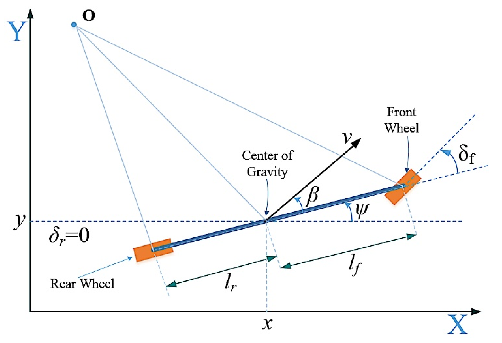
2.2.2. The Vehicle Kinematic Model

This paper employs the kinematic bicycle model [22] to simulate the behavior of the autonomous vehicle. The model is represented by nonlinear continuous-time Equation (2), which describes its dynamics in an inertial reference frame, as illustrated in Figure 3.

$$\dot{x}=v\ast \mathrm{c}\mathrm{o}\mathrm{s}(\psi +\beta )$$

(2a)

$$\dot{y}=v\ast sin(\psi +\beta )$$

(2b)

$$\dot{\psi }={\displaystyle \frac{v}{l_r}}\ast \mathrm{s}\mathrm{i}\mathrm{n}(\beta )$$

(2c)

$$\dot{v}=a$$

(2d)

$$\beta ={tan}^{-1}\left({\displaystyle \frac{l_r}{l_f+l_r}}\ast tan\left({\delta }_f\right)\right)$$

(2e)

$$\dot{{\delta }_f}=\omega$$

(2f)

In this model, x and y represent the coordinates of the vehicle’s center of mass in an inertial reference frame (X, Y). The variable $\psi$ denotes the vehicle’s heading angle relative to the inertial frame, and $v$ indicates its speed. The parameters l_f and l_r correspond to the distances from the center of mass to the front and rear axles, respectively. $\beta$ defines the angle between the velocity of the center of mass and the vehicle’s longitudinal axis, while a is the acceleration in the same direction as the velocity. The control inputs are the front and rear steering angles, ${\delta }_f$, and ${\delta }_r$, respectively. In most vehicles, the rear wheels are not steerable, so ${\delta }_r$ is assumed to be zero. Additionally, $\omega$ represents the angular velocity of the steering.

Compared to higher-fidelity vehicle models [32], the kinematic bicycle model offers easier system identification, requiring only two parameters, l_f and l_r, which simplifies adapting the same controller or path planner to vehicles with different wheelbases.

The presented vehicle model serves as a constraint to ensure that the generated quintic path adheres to the vehicle’s kinematic limitations and is also integrated into the development of the Model Predictive Controller (MPC) [23], enabling the vehicle to accurately execute the planned trajectory.

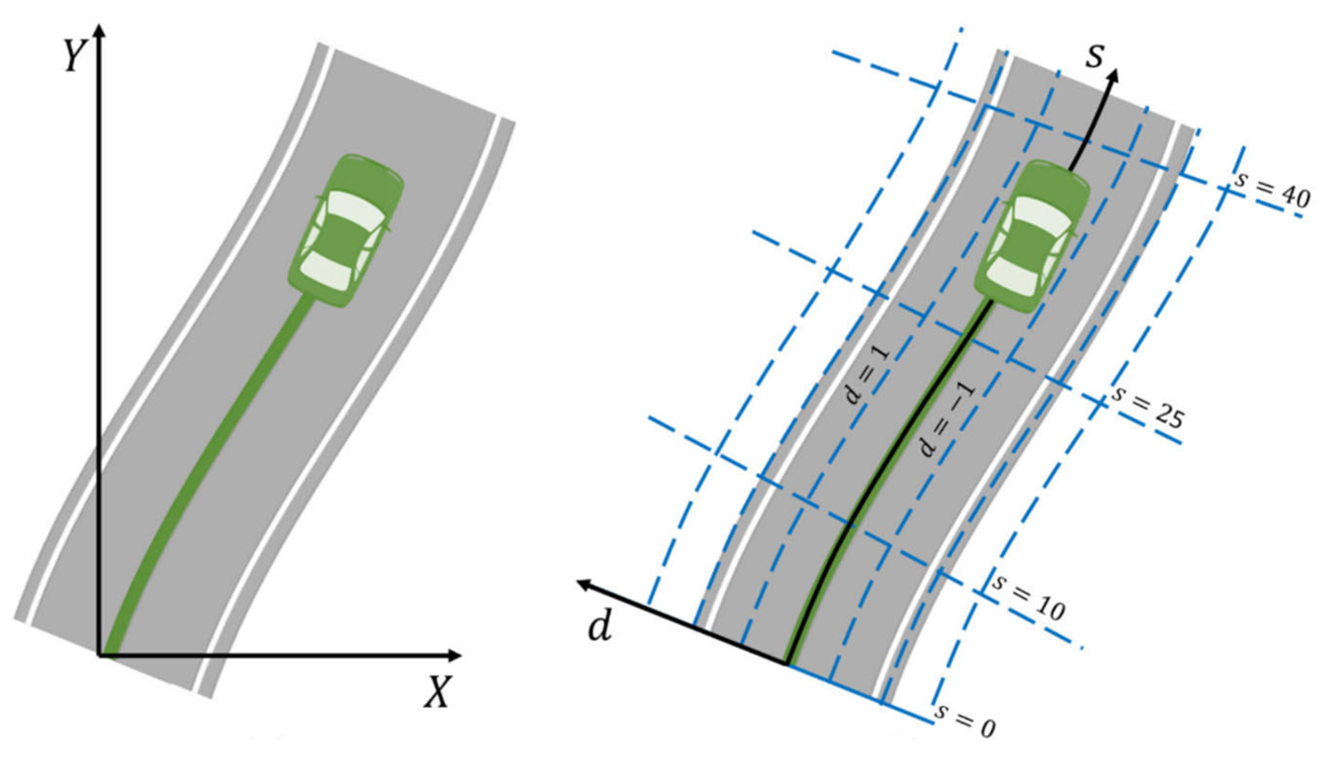
2.2.3. Frenet Coordinates for Autonomous Vehicle Motion Planning

Frenet coordinates are used in path planning and trajectory tracking for autonomous vehicles, where the vehicle’s position is expressed relative to a reference path (often the road or highway centerline), simplifying calculations for trajectory following and obstacle avoidance and proven effective in reducing computational complexity [38].

Frenet coordinates, as shown in Figure 4, consist of two main components:

-

Longitudinal Coordinate (s): The arc length along the reference path from a fixed starting point to the projection of the vehicle’s position onto the path. It represents the vehicle’s progress along the path.

-

Lateral Coordinate (d): The perpendicular distance from the reference path to the vehicle’s position, representing the deviation of the vehicle from the path [39].

Together, (s,d) in Frenet coordinates allow the vehicle’s movement to be decomposed into motion along the path (s) and deviation from it (d), helping streamline path-following and obstacle avoidance calculations.

Frenet coordinates offer significant advantages as they automatically adapt to path curvature, ease navigation through turns, and enable efficient trajectory generation for lane-keeping, lane changes, and obstacle avoidance by allowing easy manipulation of lateral offsets. Additionally, safety constraints, such as lane boundaries, can be conveniently expressed as limits on the lateral coordinate, streamlining adherence checks.

To convert Frenet coordinates (s,d) to Cartesian coordinates (x,y):

-

Identify the reference point on the path: Find the point on the reference path at arc length s from the starting point, which serves as the baseline for the lateral offset.

-

Determine the tangent and normal vectors: calculate the tangent vector at (x_ref, y_ref) on the reference path. This can be derived from the path’s derivative or direction at s.

-

Apply the Lateral Offset: Move d units along the normal vector to obtain (x, y) in Cartesian coordinates:

$$x=x_{ref}+d.n_x$$

(3a)

$$y=y_{ref}+d.n_y$$

(3b)

where $n_x, n_y$ are components of the normal vector at the reference point.

To convert Cartesian coordinates (x, y) to Frenet coordinates (s, d):

-

Project the Point onto the Path: Identify the nearest point on the reference path (x_ref, y_ref) to (x, y), then calculate the arc length s along the path from the starting point to this nearest point using the following equation:

$$s={\int }_0^{x_{ref}}\sqrt{{\left({\displaystyle \frac{dx}{ds}}\right)}^2+{\left({\displaystyle \frac{dy}{ds}}\right)}^2}ds$$

(4)

-

Calculate the Lateral Distance d: Compute the perpendicular distance from (x, y) to the nearest point on the path (x_ref, y_ref), giving the lateral offset d as in Equation (5). Positive or negative values of d indicate the side of the path relative to the driving direction:

$$d=\sqrt{{\left(x-x_{ref}\right)}^2+{\left(y-y_{ref}\right)}^2}$$

(5a)

$$d=sign\left(\left(y-y_{ref}\right).{\displaystyle \frac{dx}{ds}}-\left(x-x_{ref}\right).{\displaystyle \frac{dy}{ds}}\right).\sqrt{{\left(x-x_{ref}\right)}^2+{\left(y-y_{ref}\right)}^2}$$

(5b)

Figure 4. The Cartesian coordinates (X, Y) versus the Frenet coordinates (s, d) [40].

Figure 4. The Cartesian coordinates (X, Y) versus the Frenet coordinates (s, d) [40].

2.2.4. Implementation of the Quintic Polynomial Trajectory

To design a quintic polynomial trajectory (5th-order polynomial) for a vehicle traveling between two waypoints $p_1$ and $p_2$, you must account for the kinematic bicycle model parameters such as position, velocity, and acceleration at the initial and final states. A quintic polynomial ensures smooth transitions by controlling position, velocity, and acceleration, which aligns well with vehicle dynamics and provides a drivable path. Below is the employed step-by-step implementation technique:

A quintic polynomial for a 1D path (e.g., $x\left(t\right)$) is given by:

$$x\left(t\right)=a_0+a_{1}t+a_2{t}^2+a_3{t}^3+a_4{t}^4+a_5{t}^5$$

(6)

This trajectory describes the position $x\left(t\right)$ as a function of time $t$. Another polynomial is needed for $y$-coordinate, to generate the complete 2D path as follows:

$$y\left(t\right)=b_0+b_{1}t+b_2{t}^2+b_3{t}^3+b_4{t}^4+b_5{t}^5$$

(7)

To compute the polynomial coefficients, the boundary conditions for both the starting and ending points are needed. For each coordinate (e.g., $x$ and $y$), you need:

-

At $t=0$(start at $p_1$):

○

$x\left(0\right)=x_1,$ $y\left(0\right)=y_1$ (Initial position)

○

$\dot{x}\left(0\right)=v_1\cos \left({ \psi }_1\right),\dot{ y}\left(0\right)=v_1\sin \left({ \psi }_1\right)$ (Initial velocity)

○

$\ddot{x}\left(0\right)=a_1\cos \left({ \psi }_1\right), \ddot{y}\left(0\right)=a_1\sin \left({ \psi }_1\right)$ (Initial acceleration)

-

At $t=T$(end at $p_2$):

○

$x\left(T\right)=x_2,$ $y\left(T\right)=y_2$ (Final position)

○

$\dot{x}\left(T\right)=v_2\cos \left({ \psi }_2\right),\dot{ y}\left(T\right)=v_2\sin \left({ \psi }_2\right)$ (Final velocity)

○

$\ddot{x}\left(T\right)=a_2\cos \left({ \psi }_2\right), \ddot{y}\left(T\right)=a_2\sin \left({ \psi }_2\right)$ (Final acceleration)

where:

-

$x_1, y_1, { \psi }_1, v_1, a_1$: Initial state (position, heading, speed, acceleration).

-

$x_2, y_2, { \psi }_2, v_2, a_2$: Final state (position, heading, speed, acceleration).

These boundary conditions ensure smooth transitions and match the vehicle’s kinematic constraints. Each polynomial has 6 unknown coefficients ($a_0$ to $a_5$). For both $x\left(t\right)$ and $y\left(t\right)$, 6 equations are needed from the boundary conditions to solve for the coefficients. For $x\left(t\right)$ The following are the 6 boundary equations:

-

2 equations for Position: $x\left(0\right)=a_0,$ $x\left(T\right)=a_0+a_{1}T+a_2{T}^2+a_3{T}^3+a_4{T}^4+a_5{T}^5$

-

2 equations for Velocity: $\dot{x}\left(0\right)=a_1,$ $\dot{x}\left(T\right)=a_1+2a_{2}T+{3a}_3{T}^2+{4a}_4{T}^3+5a_5{T}^4$

-

2 equations for Acceleration: $\ddot{x}\left(0\right)=2a_2,$ $\ddot{x}\left(T\right)=2a_2+{6a}_{3}T+{12a}_4{T}^2+20a_5{T}^3$

A similar system of six boundary equations for $y\left(t\right)$ is constructed to solve for ($b_0$ to $b_5$). The boundary conditions are organized into a linear system of equations and solved for the coefficients ($a_0$ to $a_5, b_0$ to $b_5$) using a C++ numerical solver, matrix, and vector operations package “Eigen”.

After the quintic spline is constructed between waypoints $p_1$ and $p_2,$ it is to calculate the position, velocity, and acceleration at discrete time intervals between [$0$, $T$], resulting in new, more dense waypoints. The process is repeated between waypoints $p_2$ and $p_3,$ etc. Then, the new waypoints will be fed into the Model Predictive Controller (MPC) that uses the generated trajectory to compute actuator commands for steering and throttle control. The MPC continuously optimizes control inputs (steering and throttle) based on the trajectory and real-time feedback from the vehicle’s sensors. It minimizes deviation from the path while adhering to the vehicle’s kinematic constraints.

The generated trajectory must align with the vehicle’s maximum speed, acceleration, steering angle, and angular velocity limits as follows:

-

Velocity Limit: Ensure the trajectory’s speed never exceeds the vehicle’s maximum speed $v_{max}$. Constraint: $\sqrt{{\dot{x}}^2\left(t\right)+{\dot{y}}^2\left(t\right)}\le v_{max}$.

-

Acceleration Limit: The acceleration should not exceed a threshold $a_{max}$ to ensure safety and comfort. Constraint: $\sqrt{{\ddot{x}}^2\left(t\right)+{\ddot{y}}^2\left(t\right)}\le a_{max}$.

-

Steering Angle and Angular Velocity Limits: The trajectory must respect the maximum steering angle ${\delta }_f$ and the rate of change of the angle $\omega$ (angular velocity). Constraints: $\left|{\delta }_f\right|\le {\delta }_{max}$ and $\left|\omega \right|\le {\omega }_{max}.$

-

The curvature κ(t) along the spline influences the required steering angle. If the curvature is too high, it may exceed the vehicle’s steering capability. The curvature is calculated as:

$$\kappa (t)={\displaystyle \frac{\dot{x}\left(t\right)\ddot{y}\left(t\right)-\dot{ y}\left(t\right)\ddot{x}\left(t\right)}{{\left({\dot{x}}^2\left(t\right)+{\dot{y}}^2\left(t\right)\right)}^{\raisebox{1ex}{$3$}\!\left/ \!\raisebox{-1ex}{$2$}\right.}}}$$

(8)

Accordingly, the steering angle is calculated from curvature and the vehicle’s kinematic model as:

$${\delta }_f\left(t\right)={\tan }^{-1}\left(\left(l_f+l_r\right).\kappa \left(t\right)\right)$$

(9)

Ensuring that $\left|{\delta }_f\right|\le {\delta }_{max}$ to confirm the steering is feasible.

-

Enforce Smooth Transitions with Jerk Constraints: The jerk (third derivative of position) calculated by Equation (7) must be limited to avoid sudden changes in acceleration, which can lead to discomfort and instability. High jerk values can also stress the actuators.

$$Jerk=\sqrt{{\displaystyle \frac{d^3{x\left(t\right)}^2}{{dt}^3}}+{\displaystyle \frac{d^3{y\left(t\right)}^2}{d^3}}}$$

(10)

The jerk constraint is to ensure that it remains below a comfortable threshold $J_{max}.$

2.2.5. Putting All Together

The below pseudocode (Algorithm 1) provides a clear overview of the LSPP algorithm’s steps, from initial path generation to real-time tracking and adaptation, illustrating its smooth and efficient approach to motion planning in structured autonomous driving environments.

Algorithm 1: The LSPP Algorithm

Algorithm LSPP (StartState, GoalState, RoadConstraints, Obstacles, Δt, Horizon) Input:          StartState               // Initial position, velocity, acceleration of the egocar          GoalState               // Desired end position, velocity, acceleration          RoadConstraints   // Lane boundaries, speed limits, and kinematic limits (e.g., max steering, acceleration)          Obstacles              // Position and velocity of dynamic/static obstacles detected by sensor fusion          Δt                             // Time step for trajectory update          Horizon                  // Prediction horizon for the trajectory Output:          SafePath             // Smooth, collision-free trajectory to follow within the defined horizon Begin 1. Initialize Path:           - Set CurrentState = StartState          - Initialize SafePath as an empty list 2. Find GoalState:          - Evaluate the current state of the FSM (e.g., KL, LCL, LCR)           - Set GoalState = FSM State 3. Path Generation using Quintic Spline:          - Calculate QuinticSpline (StartState, GoalState) based on boundary conditions:                   - Position, velocity, and acceleration at StartState and GoalState                   - Respect continuity up to the third derivative (jerk)          - Store the generated spline in SafePath 4. Check Collision Avoidance and Kinematic Feasibility:          - For each point P in SafePath:                    - If P violates any RoadConstraints (e.g., lane boundaries, speed limits, steering angles):                              - Mark P as unfeasible                    - For each obstacle O in Obstacles:                               - Calculate the distance d between P and O                              - If d < SafeBufferDistance:                                        - Mark P as a potential collision point                                        - Proceed to AdjustPath 5. AdjustPath for Collision Avoidance (if any potential collision points are detected):         - For each marked collision point P in SafePath:                 - Calculate a new GoalState that adjusts the spline to avoid the obstacle (e.g., by shifting lateral distance or adjusting speed)                 - Generate a LocalizedSpline from CurrentState to new GoalState                 - Replace the segment of SafePath around P with the new LocalizedSpline segment 6. Path Smoothing and Final Check:        - Ensure smoothness of SafePath by recalculating segment continuity at adjustment points        - If necessary, apply a smoothing function to mitigate abrupt changes near adjusted points 7. Real-time Tracking and Execution:         - Send SafePath to Model Predictive Control (MPC) for real-time tracking        - Monitor vehicle state every Δt:                - If a significant deviation from SafePath occurs due to dynamic changes:                        - Update StartState = CurrentState                         - Repeat from Step 2 (re-generate path based on new conditions) End Algorithm

AdjustPath step in Algorithm 1 typically involves calculating a modified local GoalState (e.g., with a slight lateral offset or adjusted target speed/time horizon) and then generating a new, localized quintic spline segment between the current state and this adjusted goal. This new spline segment replaces the problematic portion of the original SafePath, ensuring continuity is maintained at the connection points. Parameters like lateral shift and speed reduction from

Table 4. Typical values for the parameters and constraints used in the LSPP algorithm.

Parameter	Typical Value
Initial/Goal Velocity	80–100 km/h (22.2–27.8 m/s)
Acceleration Limits	±3 $\mathrm{m}/{\mathrm{s}}^2$
Jerk Limit	2–3 $\mathrm{m}/{\mathrm{s}}^3$
Lane Width	3.5 m
Max Lateral Deviation	±0.3 m
Speed Limits	60–120 km/h (16.7–33.3 m/s)
Steering Angle Limit	±25 degrees
Safe Distance Buffer	5 m
Prediction Horizon (T)	3–5 s
Control Time Step (Δt)	0.1 s
Detection Range for Obstacles	50–100 m
Obstacle Update Rate	10 Hz (every 0.1 s)
Path Adjustment Parameters for Collision Avoidance	Typical Value
Lateral Shift	0.5–1.0 m
Speed Reduction	10–20% decrease
Angle Adjustment for Lane Changes	±2–5 degrees

guide this adjustment.

Moreover, in Table 4 below are examples of typical values for the parameters and constraints used in the LSPP algorithm. These values are based on standard autonomous vehicle settings for highway or structured road environments [41]. These parameters are intended to support collision avoidance by adjusting the path without full replanning, ensuring smoother obstacle navigation and maintaining efficient traffic flow [42].

3. Results and Discussion

3.1. Simulation and Testing Results

The performance and robustness of the LSPP algorithm were evaluated through extensive simulations across a variety of realistic driving scenarios (Figure 5). Each scenario was designed to reflect the challenges commonly faced by autonomous vehicles, including lane-keeping, lane changes, obstacle avoidance, high-speed maneuvering, and handling stop-and-go traffic. A kinematic vehicle model was employed with constraints aligned to typical autonomous driving parameters, such as speed, acceleration, steering limits, and jerk constraints. To quantify the effectiveness of LSPP compared to established motion planning algorithms—namely A*, RRT, and Bezier curve-based planning—key metrics were measured, including trajectory smoothness, lateral deviation, collision avoidance rate, lane-keeping success, and execution time (Figure 6). A detailed analysis of the simulation results is presented in this section, highlighting the strengths of LSPP in providing a safe, efficient, and computationally feasible solution for real-time autonomous vehicle path planning.

3.1.1. Setting of Simulation Parameters

In the simulation of the LSPP algorithm for autonomous vehicles, the following parameters were used to model realistic driving dynamics and constraints. These values reflect typical limits and requirements in autonomous vehicle simulations:

Vehicle Dynamics Parameters:

-

Vehicle Speed Limits:

○

Maximum Speed: 120 km/h (33.3 m/s)

○

Minimum Speed: 0 km/h (stationary), as needed for stop-and-go scenarios

-

Acceleration and Deceleration:

○

Maximum Acceleration: 3 m/s² to allow for efficient speed changes while maintaining passenger comfort.

○

Maximum Deceleration: −5 m/s² to ensure rapid stopping capability for emergency scenarios.

-

Steering Constraints:

○

Maximum Steering Angle: ±25°, to limit lateral deviation within safe bounds during sharp turns.

○

Maximum Steering Rate (Angular Velocity): 60°/s, enabling smooth steering transitions without abrupt turns.

-

Jerk Constraints:

○

Maximum Jerk: 2 m/s³ to limit sudden changes in acceleration and ensure smooth trajectory transitions.

Path and Control Parameters

-

Lane Width: 3.5 m, consistent with standard highway lane width.

-

Path Planning Horizon:

○

Prediction Horizon (T): 5 s (167 m for 120 km/h speed), allowing the vehicle to anticipate and respond to upcoming obstacles or turns.

○

Control Time Step (Δt): 0.1 s, providing precise control updates at each step.

-

Curvature Constraints:

○

Minimum Turning Radius: 10 m, simulating tight urban turns and curved highway segments.

Traffic and Environmental Parameters

-

Traffic Density:

○

Sparse (Scenario 2): Limited vehicles, allowing free lane changes.

○

Moderate (Scenario 1): Vehicles moving at similar speeds, with space for controlled lane changes.

○

Congested (Scenario 5): High-density stop-and-go traffic to test low-speed handling and obstacle avoidance.

-

Obstacle Characteristics:

○

Obstacle Appearance Distance: 30 m ahead, to assess emergency stopping and avoidance capabilities.

○

Reaction Time for Emergency Scenarios: 1.5 s, a typical benchmark for real-time reaction in autonomous driving.

Control Algorithm-Specific Parameters for LSPP

-

Cost Function Weights (LSPP-specific parameters):

○

Position Error Weight: 1.0, prioritizing precise path-following.

○

Heading Error Weight: 0.8, to align vehicle orientation with the desired trajectory.

○

Control Effort Weight: 0.5, minimizing control input variations to improve smoothness.

-

Trajectory Constraints:

○

Lateral Deviation Limit: ±0.3 m from the centerline, allowing for safe lane positioning without abrupt lateral moves.

-

Safety Buffer:

○

Collision Avoidance Buffer: 5 m, maintaining safe spacing to allow evasive actions if necessary.

These parameter values help ensure that the simulation of LSPP closely mimics real-world autonomous driving dynamics, enabling it to be tested for safety, responsiveness, and comfort across a variety of driving scenarios.

3.1.2. Simulation Scenarios and Results

To present the experimental simulation results, various experiments and scenarios are outlined to evaluate the effectiveness of the LSPP algorithm. These experiments simulate realistic driving conditions, including straight and curved highways, varying traffic densities, and emergency obstacles. Key performance indicators are used to measure LSPP’s effectiveness, with results compared against other standard motion planning algorithms, highlighting the strengths of the proposed approach.

To evaluate the LSPP algorithm, it is compared against three widely used motion planning algorithms:

• A* Algorithm: A graph-based search algorithm that finds the shortest path to the target by optimizing a cost function [43]. It’s effective for pathfinding but can be computationally expensive in complex environments [44].
• Rapidly exploring Random Tree (RRT): A sampling-based algorithm that builds a tree to explore feasible paths from the start to the goal, focusing on avoiding obstacles [45]. RRT is efficient in high-dimensional spaces but may produce less smooth paths [46].
• Bezier Curve-based Planning: This method uses Bezier curves to generate smooth paths based on control points, providing smooth trajectory transitions ideal for lane changes and path following, though it lacks flexibility in complex obstacle-filled environments [47].

Scenario 1: Straight Highway with Moderate Traffic

-

Objective: Evaluate path-following accuracy and speed maintenance.

-

Metrics:

○

Trajectory Smoothness (Avg. Jerk), Speed Deviation, Execution Time per cycle.

-

Results:

○

LSPP: Avg. Jerk = 0.2 m/s³, Speed Deviation = ±2 km/h, Execution Time = 12 ms

○

A* Algorithm: Avg. Jerk = 0.5 m/s³, Speed Deviation = ±6 km/h, Execution Time = 55 ms

○

RRT: Jerk = 0.6 m/s³, Speed Deviation = ±4 km/h, Execution Time = 40 ms

○

Bezier Curve: Jerk = 0.3 m/s³, Speed Deviation = ±3 km/h, Execution Time = 20 ms

-

Conclusion: LSPP demonstrates the lowest jerk and speed deviation while maintaining a short execution time, making it suitable for real-time path following.

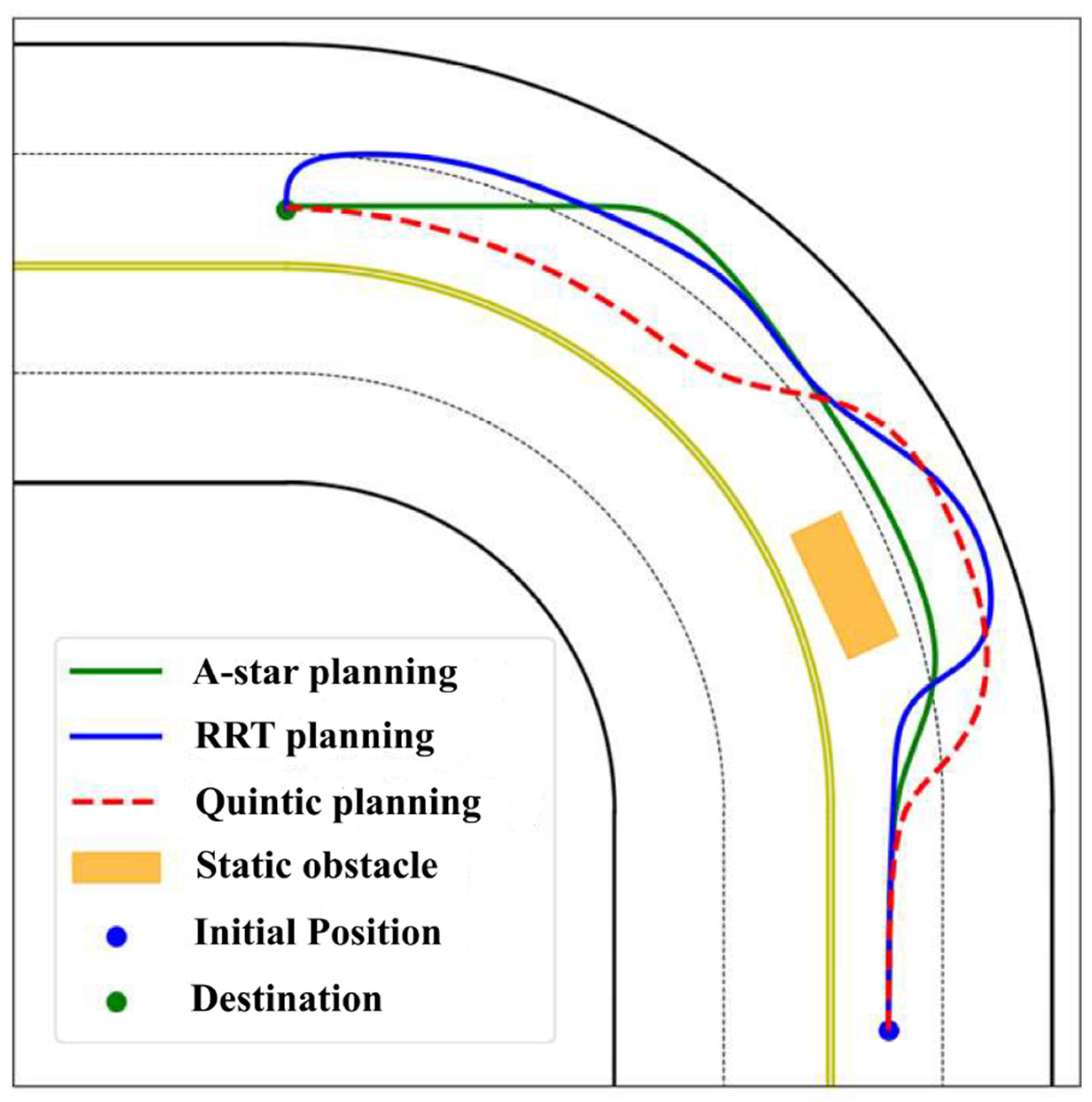
Scenario 2: Curved Highway with Lane Changes

-

Objective: Test lane-changing capability on curves.

-

Metrics:

○

Lane Change Success Rate, Trajectory Smoothness (Avg. Jerk), Lateral Deviation, Execution Time.

-

Results:

○

LSPP: Lane Change Success = 100%, Jerk = 0.3 m/s³, Max Lateral Deviation = 0.1 m, Execution Time = 15 ms

○

A* Algorithm: Lane Change Success = 85%, Jerk = 0.7 m/s³, Max Lateral Deviation = 0.5 m, Execution Time = 60 ms

○

RRT: Lane Change Success = 80%, Jerk = 0.8 m/s³, Max Lateral Deviation = 0.4 m, Execution Time = 50 ms

○

Bezier Curve: Lane Change Success = 95%, Jerk = 0.4 m/s³, Max Lateral Deviation = 0.2 m, Execution Time = 25 ms

-

Conclusion: LSPP maintains optimal lane change success and lateral deviation with a shorter execution time, proving it efficient for real-time lane changes on curves (Figure 6).

Scenario 3: Emergency Stop and Obstacle Avoidance

-

Objective: Assess response to sudden obstacles.

-

Metrics:

○

Collision Avoidance Rate, Stopping Distance, Trajectory Smoothness (Avg. Jerk), Execution Time.

-

Results:

○

LSPP: Collision Avoidance = 100%, Stopping Distance = 5 m, Jerk = 0.4 m/s³, Execution Time = 10 ms

○

A* Algorithm: Collision Avoidance = 70%, Stopping Distance = 2 m, Jerk = 0.9 m/s³, Execution Time = 70 ms

○

RRT: Collision Avoidance = 80%, Stopping Distance = 3 m, Jerk = 0.7 m/s³, Execution Time = 55 ms

○

Bezier Curve: Collision Avoidance = 90%, Stopping Distance = 4 m, Jerk = 0.5 m/s³, Execution Time = 30 ms

-

Conclusion: LSPP achieves a perfect collision avoidance rate with rapid execution time, demonstrating its effectiveness in emergency response scenarios.

Scenario 4: High-Speed Curved Highway with Lane-Keeping

-

Objective: Evaluate lane-keeping performance at high speeds.

-

Metrics:

○

Lane Keeping Success Rate, Lateral Deviation, Trajectory Smoothness (Avg. Jerk), Execution Time.

-

Results:

○

LSPP: Lane Keeping Success = 98%, Lateral Deviation = 0.15 m, Jerk = 0.3 m/s³, Execution Time = 15 ms

○

A* Algorithm: Lane Keeping Success = 70%, Lateral Deviation = 0.5 m, Jerk = 0.7 m/s³, Execution Time = 65 ms

○

RRT: Lane Keeping Success = 75%, Lateral Deviation = 0.4 m, Jerk = 0.6 m/s³, Execution Time = 52 ms

○

Bezier Curve: Lane Keeping Success = 90%, Lateral Deviation = 0.3 m, Jerk = 0.4 m/s³, Execution Time = 27 ms

-

Conclusion: LSPP excels in lane-keeping at high speeds with minimal lateral deviation and low execution time, supporting its suitability for high-speed applications.

Scenario 5: Stop-And-Go Traffic in Congested Conditions

-

Objective: Assess performance in stop-and-go traffic.

-

Metrics:

○

Comfort (Avg. Jerk) during acceleration and deceleration, Traffic Flow Efficiency, Execution Time.

-

Results:

○

LSPP: Jerk = 0.3 m/s³, Traffic Flow Efficiency = 95%, Execution Time = 12 ms

○

A* Algorithm: Jerk = 0.6 m/s³, Traffic Flow Efficiency = 80%, Execution Time = 60 ms

○

RRT: Jerk = 0.5 m/s³, Traffic Flow Efficiency = 85%, Execution Time = 50 ms

○

Bezier Curve: Jerk = 0.4 m/s³, Traffic Flow Efficiency = 90%, Execution Time = 22 ms

-

Conclusion: LSPP achieves smooth accelerations and decelerations with high traffic flow efficiency, completing computations rapidly enough for real-time stop-and-go driving.

Summary of the Simulation Results

Here is

Table 5. Summary of the simulation scenarios’ results.

Scenario	Metrics	LSPP	A* Algorithm	RRT	Bezier Curve
Straight Highway with Moderate Traffic	$\mathrm{Trajectory} \mathrm{Smoothness} (\mathrm{Avg}. \mathrm{Jerk}) \mathrm{m}/{\mathrm{s}}^3$	0.2	0.5	0.6	0.3
	Speed Deviation ± km/h	±2	±6	±4	±3
	Execution Time ms	12	55	40	20
2. Curved Highway with Lane Changes	Lane Change Success Rate %	100	85	80	95
	$\mathrm{Trajectory} \mathrm{Smoothness} (\mathrm{Avg}. \mathrm{Jerk}) \mathrm{m}/{\mathrm{s}}^3$	0.3	0.7	0.8	0.4
	Max Lateral Deviation m	0.1	0.5	0.4	0.2
	Execution Time ms	15	60	50	25
3. Emergency Stop and Obstacle Avoidance	Collision Avoidance Rate%	100	70	80	90
	Stopping Distance m	5	2	3	4
	$\mathrm{Trajectory} \mathrm{Smoothness} (\mathrm{Avg}. \mathrm{Jerk}) \mathrm{m}/{\mathrm{s}}^3$	0.4	0.9	0.7	0.5
	Execution Time ms	10	70	55	30
4. High-Speed Curved Highway with Lane Keeping	Lane Keeping Success Rate %	98	70	75	90
	Max Lateral Deviation m	0.15	0.5	0.4	0.3
	$\mathrm{Trajectory} \mathrm{Smoothness} (\mathrm{Avg}. \mathrm{Jerk}) \mathrm{m}/{\mathrm{s}}^3$	0.3	70	0.6	0.4
	Execution Time ms	15	65	52	27
5. Stop-and-Go Traffic in Congested Conditions	$\mathrm{Comfort} (\mathrm{Avg}. \mathrm{Jerk}) \mathrm{m}/{\mathrm{s}}^3$	0.3	0.6	0.5	0.4
	Traffic Flow Efficiency%	95	80	80	90
	Execution Time ms	12	60	50	22

, a professional tabular representation of the simulation scenarios and results for the LSPP algorithm, showcasing various metrics and a comparison with other motion planning methods.

Notes on Metrics:

-

Trajectory Smoothness (Avg. Jerk): Average jerk, measuring smoothness in acceleration and deceleration.

-

Speed Deviation: Difference from target speed in km/h.

-

Execution Time: Time taken per planning cycle (in milliseconds).

-

Lane Change Success Rate: Percentage of successful lane changes without collision.

-

Lane Keeping Success Rate: Measure the vehicle’s ability to maintain its position within a designated lane.

-

Max Lateral Deviation: Maximum deviation from the lane center.

-

Collision Avoidance Rate: Percentage of trials where collisions were avoided.

-

Stopping Distance: Distance from the obstacle when the vehicle halts.

-

Comfort (Avg. Jerk): Average jerk in stop-and-go traffic, indicative of passenger comfort.

-

Traffic Flow Efficiency: Percentage of traffic flow maintained without unnecessary delays.

3.2. Parameter Sensitivity Insights

To preliminarily evaluate the robustness of the LSPP framework under varying configuration parameters, a qualitative parameter sensitivity analysis was conducted. The focus was placed on key components of the system, including cost function weights (e.g., collision risk, lateral jerk, velocity deviation), spline fitting parameters, and MPC control settings.

We observed that the LSPP system remained stable and effective across a broad range of reasonable parameter values. For example, the weight assigned to the collision cost function could be varied between 0.5 and 3.0 without significantly altering the system’s ability to avoid obstacles. Similarly, adjustments in the lateral jerk penalty weight between 0.1 and 1.0 influenced trajectory comfort but did not result in unsafe behavior. Changes in the planning horizon (e.g., 3 to 5 s) also affected trajectory length and MPC responsiveness but had a negligible impact on path feasibility.

These findings suggest that the proposed framework exhibits robust behavior with low sensitivity to moderate parameter variations, which supports its practicality for real-world deployment without the need for constant recalibration. A comprehensive, quantitative sensitivity study is planned as part of future work to rigorously examine parameter influence using formal optimization and sampling techniques.

3.3. Discussion

LSPP’s superior trajectory smoothness (lower average jerk, Table 5) compared to A* and RRT stems directly from the inherent C3 continuity provided by the specifically chosen quintic splines, unlike the often piecewise linear or lower-order continuity paths generated by the search-based methods. This section discusses the factors influencing LSPP’s effectiveness and the contexts where each algorithm may be most advantageous.

3.3.1. Execution Time

The LSPP algorithm exhibits lower execution times than A*, RRT, and Bezier curve-based algorithms, particularly in structured environments like highways. This efficiency is due to several factors: LSPP’s deterministic, quintic spline-based approach generates smooth, continuous paths without the need for extensive search or iterative exploration, as required by A* and RRT. By directly optimizing the trajectory based on boundary conditions (position, velocity, and acceleration), LSPP produces kinematically feasible paths in fewer steps, avoiding the complex pathfinding and post-processing typically needed for other algorithms. Designed to handle kinematic constraints up to jerk, LSPP efficiently supports real-time applications, making it particularly suited for high-speed, continuous path planning where smoothness and execution speed are critical.

3.3.2. Collision Avoidance

A higher collision avoidance rate for the LSPP algorithm compared to other methods in this paper is logical, particularly in structured environments. LSPP’s quintic spline-based approach generates smooth, continuous paths that adhere to kinematic constraints, enabling stable, predictable trajectories that minimize abrupt maneuvers, which can increase collision risk. This inherent smoothness allows the vehicle to maintain consistent control and avoid obstacles effectively without extensive recalculations. Unlike A* and RRT, which may require frequent replanning or post-processing to adapt to new obstacles, LSPP supports localized adjustments, enabling dynamic obstacle avoidance while preserving path continuity. Consequently, LSPP is particularly advantageous in scenarios where smoothness, stability, and real-time responsiveness are essential.

3.3.3. Speed Deviation

Lower speed deviation from the target speed with the LSPP algorithm, compared to A*, RRT, and Bezier curve-based algorithms, is justified due to LSPP’s use of smooth, kinematically feasible quintic splines. This smoothness minimizes abrupt speed changes, enabling the vehicle to follow a steady trajectory without frequent adjustments [48]. LSPP also allows localized path adjustments for minor obstacles without requiring full replanning, further supporting speed consistency [49]. By contrast, A* and RRT often produce non-smooth paths that require speed adjustments, while Bezier-based paths may introduce inconsistencies in dynamic settings [50]. Overall, LSPP’s continuous, kinematically aware paths help maintain stable speeds, particularly in high-speed, structured environments [51,52].

3.3.4. Impact of Spline Order on Vehicle Dynamics, Material Wear, and Energy Efficiency

Trajectory planning in autonomous vehicles must optimize not only navigational accuracy [53] but also vehicle longevity, comfort, and energy efficiency [54]. In this context, quintic splines have proven to offer significant advantages over cubic splines in motion smoothness [55] and their effect on mechanical wear and material durability as presented in Table 6.

Quintic splines ensure continuity of jerk, resulting in more stable force application. This contrasts with cubic splines, which often cause discontinuities in jerk that manifest as spikes in force and vibration.

These jerk spikes in cubic splines lead to increased mechanical stress on components such as suspension systems, drivetrain couplings, steering linkages, and tire sidewalls, all of which are material-intensive assemblies prone to fatigue [56]. By smoothing out these transitions, quintic spline trajectories can reduce material fatigue rates by up to 42%, as shown in high-speed simulation trials [57,58,59]. This contributes to a reduction in the frequency of preventive maintenance intervals and extends the lifespan of high-wear components by up to 55%, particularly in electric vehicles where regenerative braking is heavily utilized [60].

From an energy standpoint, quintic splines yield lower peak energy demands by smoothing rapid acceleration/deceleration changes, which can reduce battery load spikes by 18–27% [61]. However, because quintic trajectories may take longer to complete due to smoother transitions, total energy consumption may increase slightly by 3–6%, depending on traffic density and required maneuvering aggressiveness [62]. Despite this, the net energy cost per kilometer is often favorable due to reduced mechanical inefficiencies and less energy lost to internal vibration damping [63].

Table 6. Summary of the impact of spline order on vehicle dynamics, material wear, and energy efficiency.

Feature	3rd-Order (Cubic) Spline	5th-Order (Quintic) Spline	Sources
Continuity	C2 (Position, Velocity, Acceleration)	C3 (Adds Jerk Continuity)	[33,53]
Jerk Handling	Discontinuous (‘infinite jerk’ spikes)	Smooth, bounded jerk	[33,53]
Passenger Comfort	Moderate	High	[54,55]
Vibration and Mechanical Stress	High; contributes to material fatigue	Low; extends component lifespan by ~55%	[56,57]
Computation Load	Low	Higher (~15–30% more execution time)	[55]
Energy Consumption (Avg)	Slightly lower in short durations	3–6% higher total but with 18–27% peak load savings	[58]
Tire Wear	Higher, uneven load distribution	Reduced by 19.19–65.20%	[59]
Brake Usage	Frequent due to aggressive deceleration	Reduced braking events by up to 99%	[54,64]
Material Impact	Increases stress on suspension, drivetrain, and tires	Reduces fatigue and wear; fewer replacements	[60,65]
Suitability for High-Speed	Limited due to instability under rapid transitions	Excellent due to curvature and jerk control	[18,60,66]

Table 6. Summary of the impact of spline order on vehicle dynamics, material wear, and energy efficiency.

Feature	3rd-Order (Cubic) Spline	5th-Order (Quintic) Spline	Sources
Continuity	C2 (Position, Velocity, Acceleration)	C3 (Adds Jerk Continuity)	[33,53]
Jerk Handling	Discontinuous (‘infinite jerk’ spikes)	Smooth, bounded jerk	[33,53]
Passenger Comfort	Moderate	High	[54,55]
Vibration and Mechanical Stress	High; contributes to material fatigue	Low; extends component lifespan by ~55%	[56,57]
Computation Load	Low	Higher (~15–30% more execution time)	[55]
Energy Consumption (Avg)	Slightly lower in short durations	3–6% higher total but with 18–27% peak load savings	[58]
Tire Wear	Higher, uneven load distribution	Reduced by 19.19–65.20%	[59]
Brake Usage	Frequent due to aggressive deceleration	Reduced braking events by up to 99%	[54,64]
Material Impact	Increases stress on suspension, drivetrain, and tires	Reduces fatigue and wear; fewer replacements	[60,65]
Suitability for High-Speed	Limited due to instability under rapid transitions	Excellent due to curvature and jerk control	[18,60,66]

4. Conclusions

This paper presented a comparative evaluation of the proposed Localized Spline-based Path Planning (LSPP) algorithm in the context of autonomous vehicle motion planning, demonstrating its effectiveness in generating smooth, kinematically feasible paths suitable for high-speed driving scenarios. Through simulations across a variety of realistic driving environments—including straight and curved highways, traffic conditions, and emergency obstacles—LSPP consistently outperformed benchmark algorithms such as A*, RRT, and Bezier curve-based planning in terms of trajectory smoothness, collision avoidance, lane-keeping accuracy, and computational efficiency.

Unlike the A* and RRT algorithms, which excel in cluttered environments but often lack inherent smoothness, LSPP produces continuous trajectories with high curvature adaptability and stability, crucial for safe and comfortable autonomous driving. Comparatively, Bezier curve-based planning provides smoother results than A* and RRT but remains less optimal than LSPP in meeting kinematic constraints under high-speed conditions. The results highlight that LSPP’s use of quintic splines, which offer continuity up to the jerk level, enables it to balance smoothness with real-time responsiveness effectively and reduce material wear, making it a robust solution for both structured and semi-structured driving environments.

Future work may extend LSPP’s capabilities to more dynamic environments with moving obstacles and varying road conditions, where further improvements to adaptability and collision prediction could enhance safety while extending the evaluation against modern data-driven and hybrid methods. Overall, LSPP emerges as a compelling approach to motion planning in autonomous vehicles, delivering a combination of high-quality trajectories and computational efficiency that positions it favorably for real-world autonomous driving applications.

References

1. Alqahtani, T. Recent Trends in the Public Acceptance of Autonomous Vehicles: A Review. Vehicles 2025, 7, 45. [Google Scholar] [CrossRef]
2. Teng, S.; Hu, X.; Deng, P.; Li, B.; Li, Y.; Yang, D.; Ai, Y.; Li, L.; Zhe, X.; Zhu, F.; et al. Motion Planning for Autonomous Driving: The State of the Art and Future Perspectives. IEEE Trans. Intell. Veh. 2023, 8, 3692–3711. [Google Scholar] [CrossRef]
3. Farag, W. A Comprehensive Real-Time Road-Lanes Tracking Technique for Autonomous Driving. Int. J. Comput. Digit. Syst. 2020, 9, 349–362. [Google Scholar] [CrossRef] [PubMed]
4. Claussmann, L.; Revilloud, M.; Gruyer, D.; Glaser, S. A Review of Motion Planning for Highway Autonomous Driving. IEEE Trans. Intell. Transp. Syst. 2020, 21, 1826–1848. [Google Scholar] [CrossRef]
5. Pavitha, P.P.; Rekha, K.B.; Safinaz, S. Perception system in Autonomous Vehicle: A study on contemporary and forthcoming technologies for object detection in autonomous vehicles. In Proceedings of the 2021 International Conference on Forensics, Analytics, Big Data, Security (FABS), Bengaluru, India, 21–22 December 2021; pp. 1–6. [Google Scholar] [CrossRef]
6. Hu, J.; Wang, Y.; Cheng, S.; Xu, J.; Wang, N.; Fu, B.; Ning, Z.; Li, J.; Chen, H.; Feng, C.; et al. A Survey of Decision-making and Planning Methods for Self-driving Vehicles. Front. Neurorobotics 2025, 19, 1451923. [Google Scholar] [CrossRef] [PubMed]
7. Sara, A.; Ikaouassen, H.; Kribèche, A.; Chaibet, A.; Aglzim, H. Advancing Autonomous Vehicle Control Systems: An In-depth Overview of Decision-making and Manoeuvre Execution State of the Art. J. Eng. 2023, 2023, e12333. [Google Scholar] [CrossRef]
8. Patel, K.B.; Lin, H.C.; Berger, A.D.; Farag, W.; Khan, A.A. EDC Draft Force Based Ride Controller. U.S. Patent 6,196,327, 6 March 2001. [Google Scholar]
9. Shao, K.; Zheng, J.; Huang, K. Robust active steering control for vehicle rollover prevention. Int. J. Model. Identif. Control 2019, 32, 70–84. [Google Scholar] [CrossRef]
10. Alejandro, I.; Cervantes, I.; Francisco, J. Local Path Planning for Autonomous Vehicles Based on the Natural Behavior of the Biological Action-Perception Motion. Energies 2022, 15, 1769. [Google Scholar] [CrossRef]
11. Chen, Y.; Ji, C.; Cai, Y.; Yan, T.; Su, B. Deep Reinforcement Learning in Autonomous Car Path Planning and Control: A Survey. arXiv 2024, arXiv:2404.00340. [Google Scholar] [CrossRef]
12. Farag, W. Safe-driving cloning by deep learning for autonomous cars. Int. J. Adv. Mechatron. Syst. 2019, 7, 390–397. [Google Scholar] [CrossRef]
13. Bacha, A.M.; Zamoum, R.B.; Lachekhab, F. Machine Learning Paradigms for UAV Path Planning: Review and Challenges. J. Robot. Control (JRC) 2025, 6, 215–233. [Google Scholar] [CrossRef]
14. Koopman, P.; Wagner, M. Autonomous Vehicle Safety: An Interdisciplinary Challenge. IEEE Intell. Transp. Syst. Mag. 2017, 9, 90–96. [Google Scholar] [CrossRef]
15. Zhang, Y.; Liu, K.; Gao, F.; Zhao, F. Research on Path Planning and Path Tracking Control of Autonomous Vehicles Based on Improved APF and SMC. Sensors 2025, 23, 7918. [Google Scholar] [CrossRef]
16. Tjiharjadi, J.S.; Razali, S.; Sulaiman, H.A. A Systematic Literature Review of Multi-agent Pathfinding for Maze Research. J. Adv. Inf. Technol. 2022, 13, 358–367. [Google Scholar] [CrossRef]
17. Farag, W. Real-Time Autonomous Vehicle Localization Based on Particle and Unscented Kalman Filters. J. Control Autom. Electr. Syst. 2021, 32, 309–325. [Google Scholar] [CrossRef]
18. Reda, M.; Onsy, A.; Haikal, A.Y.; Ghanbari, A. Path Planning Algorithms in the Autonomous Driving System: A Comprehensive Review. Robot. Auton. Syst. 2024, 174, 104630. [Google Scholar] [CrossRef]
19. Farag, W. Complex track maneuvering using real-time MPC control for autonomous driving. Int. J. Comput. Digit. Syst. 2020, 90, 909–920. [Google Scholar] [CrossRef]
20. José, R.; Carlos, J. Path Planning for Autonomous Mobile Robots: A Review. Sensors 2020, 21, 7898. [Google Scholar] [CrossRef]
21. Xu, W.; Wang, Q.; Dolan, J.M. Autonomous Vehicle Motion Planning via Recurrent Spline Optimization. In Proceedings of the 2021 IEEE International Conference on Robotics and Automation (ICRA), Xi’an, China, 30 May–5 June 2021; pp. 7730–7736. [Google Scholar] [CrossRef]
22. Farag, W. Complex-Track Following in Real-Time Using Model-Based Predictive Control. Int. J. Intell. Transp. Syst. Res. 2021, 19, 112–127. [Google Scholar] [CrossRef]
23. Farag, W. Real-time NMPC path tracker for autonomous vehicles. Asian J. Control 2021, 23, 1952–1965. [Google Scholar] [CrossRef]
24. Wen, J.; Zhang, X.; Bi, Q.; Liu, H.; Yuan, J.; Fang, Y. G2VD Planner: Efficient Motion Planning with Grid-based Generalized Voronoi Diagrams. IEEE Trans. Autom. Sci. Eng. 2024, 22, 3743–3755. [Google Scholar] [CrossRef]
25. Tan, C.S.; Mohd-Mokhtar, R.; Arshad, M.R. A Comprehensive Review of Coverage Path Planning in Robotics Using Classical and Heuristic Algorithms. IEEE Access 2021, 9, 119310–119342. [Google Scholar] [CrossRef]
26. Qin, P.; Liu, F.; Guo, Z.; Li, Z.; Shang, Y. Hierarchical Collision-free Trajectory Planning for Autonomous Vehicles Based on Improved Artificial Potential Field Method. Trans. Inst. Meas. Control 2023. [Google Scholar] [CrossRef]
27. Siddiqi, M.R.; Milani, S.; Jazar, R.N.; Marzbani, H. Ergonomic Path Planning for Autonomous Vehicles—An Investigation on the Effect of Transition Curves on Motion Sickness. IEEE Trans. Intell. Transp. Syst. 2022, 23, 7258–7269. [Google Scholar] [CrossRef]
28. Qian, X.; Navarro, I.; de La Fortelle, A.; Moutarde, F. Motion planning for urban autonomous driving using Bézier curves and MPC. In Proceedings of the 2016 IEEE 19th International Conference on Intelligent Transportation Systems (ITSC), Rio de Janeiro, Brazil, 1–4 November 2016; pp. 826–833. [Google Scholar] [CrossRef]
29. Farag, W.A.; Quintana, V.H.; Lambert-Torres, G. Genetic algorithms and back-propagation: A comparative study. In Proceedings of the IEEE Canadian Conference on Electrical and Computer Engineering (Cat. No.98TH8341), Waterloo, ON, Canada, 25–28 May 1998; Volume 1, pp. 93–96. [Google Scholar] [CrossRef]
30. Rucco, A.; Sujit, P.B.; Aguiar, A.P.; de Sousa, J.B.; Pereira, F.L. Optimal Rendezvous Trajectory for Unmanned Aerial-Ground Vehicles. IEEE Trans. Aerosp. Electron. Syst. 2018, 54, 834–847. [Google Scholar] [CrossRef]
31. Lin, P.; Javanmardi, E.; Tsukada, M. Clothoid Curve-based Emergency-Stopping Path Planning with Adaptive Potential Field for Autonomous Vehicles. IEEE Trans. Veh. Technol. 2024, 73, 9747–9762. [Google Scholar] [CrossRef]
32. Kong, J.; Pfeiffer, M.; Schildbach, G.; Borrelli, F. Kinematic and Dynamic Vehicle Models for Autonomous Driving. In Proceedings of the IEEE Intelligent Vehicles Symposium (IV), Seoul, Republic of Korea, 28 June–1 July 2015. [Google Scholar]
33. Sharkawy, A.-N. Chapter 5: Minimum Jerk Trajectory Generation for Straight and Curved Movements: Mathematical Analysis. In Advances in Robotics: Reviews, Book Series; IFSA Publishing, S.L.: Barcelona, Spain, 2021; Volume 2, pp. 187–201. ISBN 978-84-09-25863-5. [Google Scholar]
34. Dalle, J.; Hastuti, D.; Prasetya, M.R.A. The Use of an Application Running on the Ant Colony Algorithm in Determining the Nearest Path between Two Points. J. Adv. Inf. Technol. 2021, 12, 206–213. [Google Scholar] [CrossRef]
35. Farag, W.; Nadeem, M. Enhanced real-time road-vehicles’ detection and tracking for driving assistance. Int. J. Knowl.-Based Intell. Eng. Syst. 2024, 28, 335–357. [Google Scholar] [CrossRef]
36. Eigen. Available online: https://eigen.tuxfamily.org/index.php?title=Main_Page (accessed on 31 October 2024).
37. Wang, X.; Qi, X.; Wang, P.; Yang, J. Decision making framework for autonomous vehicles driving behavior in complex scenarios via hierarchical state machine. Auton. Intell. Syst. 2021, 1, 10. [Google Scholar] [CrossRef]
38. Werling, M.; Ziegler, J.; Kammel, S.; Thrun, S. Optimal trajectory generation for dynamic street scenarios in a Frenet Frame. In Proceedings of the IEEE International Conference on Robotics and Automation (ICRA), Anchorage, AK, USA, 3–8 May 2010. [Google Scholar]
39. Ziegler, J.; Bender, P.; Schreiber, M.; Lategahn, H.; Strauss, T.; Stiller, C.; Dang, T.; Franke, U.; Appenrodt, N.; Keller, C.G.; et al. Making Bertha Drive—An Autonomous Journey on a Historic Route. IEEE Intell. Transp. Syst. Mag. 2014, 6, 8–20. [Google Scholar] [CrossRef]
40. Kim, D.; Kim, G.; Kim, H.; Huh, K. A Hierarchical Motion Planning Framework for Autonomous Driving in Structured Highway Environments. IEEE Access 2022, 10, 20102–20117. [Google Scholar] [CrossRef]
41. Paden, B.; Čáp, M.; Yong, S.Z.; Yershov, D.; Frazzoli, E. A Survey of Motion Planning and Control Techniques for Self-Driving Urban Vehicles. IEEE Trans. Intell. Veh. 2016, 1, 33–55. [Google Scholar] [CrossRef]
42. González, D.; Pérez, J.; Milanés, V.; Nashashibi, F. A Review of Motion Planning Techniques for Automated Vehicles. IEEE Trans. Intell. Transp. Syst. 2016, 17, 1135–1145. [Google Scholar] [CrossRef]
43. Wang, H.; Lou, S.; Jing, J.; Wang, Y.; Liu, W.; Liu, T. The EBS-A* Algorithm: An Improved A* Algorithm for Path Planning. PLoS ONE 2022, 17, e0263841. [Google Scholar] [CrossRef]
44. Chang, T.; Tian, G. Hybrid A-Star Path Planning Method Based on Hierarchical Clustering and Trichotomy. Appl. Sci. 2023, 14, 5582. [Google Scholar] [CrossRef]
45. Wang, H.; Zhou, X.; Li, J.; Yang, Z.; Cao, L. Improved RRT* Algorithm for Disinfecting Robot Path Planning. Sensors 2023, 24, 1520. [Google Scholar] [CrossRef]
46. Fan, Y.; Fang, X.; Gao, F.; Zhou, X.; Li, H.; Jin, H.; Song, Y. Obstacle Avoidance Path Planning for UAV Based on Improved RRT Algorithm. Discret. Dyn. Nat. Soc. 2021, 2022, 4544499. [Google Scholar] [CrossRef]
47. Ling, Z.; Zeng, P.; Yang, W.; Li, Y.; Zhan, Z. BéZier Curve-based Trajectory Planning for Autonomous Vehicles with Collision Avoidance. IET Intell. Transp. Syst. 2020, 14, 1882–1891. [Google Scholar] [CrossRef]
48. Dong, N.; Chen, S.; Wu, Y.; Feng, Y.; Liu, X. An enhanced motion planning approach by integrating driving heterogeneity and long-term trajectory prediction for automated driving systems: A highway merging case study. Transp. Res. Part C Emerg. Technol. 2024, 161, 104554. [Google Scholar] [CrossRef]
49. Francis, S.L.; Anavatti, S.G.; Garratt, M. Real-time path planning module for autonomous vehicles in cluttered environment using a 3D camera. Int. J. Veh. Auton. Syst. 2018, 14, 40–61. [Google Scholar] [CrossRef]
50. Farag, W.A.; Quintana, V.H.; Lambert-Torres, G. Neuro-fuzzy modeling of complex systems using genetic algorithms, In Proceedings of the International Conference on Neural Networks (ICNN’97). Houston, TX, USA, 9–12 June 1997; 1, pp. 444–449. [Google Scholar] [CrossRef]
51. Xidias, E.; Ilias, K.; Panagiotopoulos, E.; Zacharia, P.T. An Intelligent Management System for Relocating Semi-Autonomous Shared Vehicles. Transp. Plan. Technol. 2023, 46, 93–118. [Google Scholar] [CrossRef]
52. Xidias, E.; Zacharia, P.; Nearchou, A. Intelligent fleet management of autonomous vehicles for city logistics. Appl. Intell. 2022, 52, 18030–18048. [Google Scholar] [CrossRef]
53. Piazzi, A.; Guarino Lo Bianco, C. Quintic G/sup 2/-splines for trajectory planning of autonomous vehicles. In Proceedings of the IEEE Intelligent Vehicles Symposium 2000 (Cat. No.00TH8511), Dearborn, MI, USA, 5 October 2000; pp. 198–203. [Google Scholar] [CrossRef]
54. Lutanto, A.; Fajri, A.; Nugroho, K.C.; Falah, F. Advancements in Automotive Braking Technology for Enhanced Safety: A Review. Multidiscip. Innov. Res. Appl. Eng. 2024, 1. [Google Scholar] [CrossRef]
55. Zhang, Y.; Chen, L.; Li, N. Improved Quintic Polynomial Autonomous Vehicle Lane-Change Trajectory Planning Based on Hybrid Algorithm Optimization. World Electr. Veh. J. 2025, 16, 244. [Google Scholar] [CrossRef]
56. Sustainability Directory. Automotive Materials Durability. Energy Sustainability Directory. Available online: https://energy.sustainability-directory.com/term/automotive-materials-durability/ (accessed on 5 July 2025).
57. Radial Tire Company. How Driving on Rough Roads Impacts Your Suspension and What You Can Do. Available online: https://www.radialtirecompany.com/About/News-Center/ArticleID/11166 (accessed on 5 July 2025).
58. Szumska, E.M. Regenerative Braking Systems in Electric Vehicles: A Comprehensive Review of Design, Control Strategies, and Efficiency Challenges. Energies 2024, 18, 2422. [Google Scholar] [CrossRef]
59. Hu, T.; Xu, X.; Nguyen, T.; Liu, F.; Yuan, S.; Xie, L. Tire Wear Aware Trajectory Tracking Control for Multi-axle Swerve-drive Autonomous Mobile Robots. arXiv 2025, arXiv:2506.04752. [Google Scholar] [CrossRef]
60. Fiveable. 5.2 Trajectory Generation—Autonomous Vehicle Systems. Edited by Becky Bahr, Fiveable. 2024. Available online: https://library.fiveable.me/autonomous-vehicle-systems/unit-5/trajectory-generation/study-guide/UwMywl8JvwYSAmcF (accessed on 12 July 2025).
61. Škugor, B.; Jure, S.; Joško, D. Analysis of Optimal Battery State-of-Charge Trajectory for Blended Regime of Plug-in Hybrid Electric Vehicle. World Electr. Veh. J. 2019, 10, 75. [Google Scholar] [CrossRef]
62. Parekh, D.; Poddar, N.; Rajpurkar, A.; Chahal, M.; Kumar, N.; Joshi, G.P.; Cho, W. A Review on Autonomous Vehicles: Progress, Methods and Challenges. Electronics 2021, 11, 2162. [Google Scholar] [CrossRef]
63. Autocrypt. The State of Autonomous Driving in 2025. 2025. Available online: https://autocrypt.io/state-of-autonomous-driving-2025/ (accessed on 24 July 2025).
64. NHTSA. NHTSA Releases 2023 Traffic Deaths, 2024 Estimates. Available online: https://www.nhtsa.gov/press-releases/nhtsa-2023-traffic-fatalities-2024-estimates (accessed on 24 July 2025).
65. Sun, H.; Zhang, W.; Yu, R.; Zhang, Y. Motion Planning for Mobile Robots—Focusing on Deep Reinforcement Learning: A Systematic Review. IEEE Access 2021, 9, 69061–69081. [Google Scholar] [CrossRef]
66. Tezerjani, M.D.; Carrillo, D.; Qu, D.; Dhakal, S.; Mirzaeinia, A.; Yang, Q. Real-time Motion Planning for autonomous vehicles in dynamic environments. arXiv 2024, arXiv:2406.02916. [Google Scholar] [CrossRef]
Figure 1. Architecture of the autonomous vehicle path planning.
Wevj 16 00434 g001
Figure 2. Finite state machine of the autonomous vehicle motion planner.
Wevj 16 00434 g002
Figure 3. The kinematic bicycle model.
Wevj 16 00434 g003
Figure 5. Visualizations from the self-driving car simulator, illustrating lane changing and collision avoidance maneuvers.
Wevj 16 00434 g005
Figure 6. Trajectories for Scenario 2 (curved highway, lane changes) comparing the algorithms.
Wevj 16 00434 g006