Spatial Diagnosis of Climatic and Landscape Controls on Forest Leaf Area Index Across China Using Interpretable Machine Learning

Abstract

Forest cover condition is a key determinant of ecosystem functioning and ecological resilience, yet its spatial variability across large and environmentally heterogeneous regions remains insufficiently understood. Leaf area index (LAI) provides a continuous and physically meaningful indicator of forest canopy condition, reflecting variations in canopy density associated with climate and landscape structure. Here, we develop a spatially explicit and interpretable analytical framework to diagnose the dominant climatic and landscape controls on forest cover condition across mainland China during 2000–2020. By integrating machine-learning modelling with SHapley Additive exPlanations, GeoDetector interaction analysis, and nonlinear dependence diagnostics, we quantify the relative contributions and interactions of precipitation, temperature, topography, and forest landscape structure to spatial patterns in forest LAI. The results reveal pronounced spatial heterogeneity in forest cover control regimes. Precipitation dominates forest cover condition in humid regions but exhibits nonlinear saturation, whereas forest fragmentation strongly constrains canopy development and moderates climate-LAI relationships in arid and semi-arid forested landscapes. In high-elevation regions, topographic and thermal factors exert primary control. Overall, the findings demonstrate that forest cover condition reflects climate-conditioned and landscape-dependent control regimes, providing a transparent basis for large-scale forest cover assessment and ecological monitoring.

1. Introduction

Leaf Area Index (LAI), defined as the one-sided green leaf area per unit ground surface area, is a fundamental indicator of vegetation structure and ecosystem functioning [1]. By regulating photosynthesis, transpiration, and surface energy exchange, LAI plays a central role in mediating land–atmosphere interactions and ecosystem productivity. Consequently, LAI has become a widely used metric in ecological assessment, land-use planning, and applied environmental analysis, particularly in the context of climate change and increasing anthropogenic pressure on terrestrial ecosystems [2].

Direct field-based measurements of LAI, although essential for calibration and validation, are limited by spatial coverage, operational costs, and sensitivity to canopy structure and observer bias [3]. Satellite remote sensing has therefore become the primary means of monitoring LAI dynamics over large spatial and temporal scales. Long-term satellite products have revealed substantial changes in vegetation cover and canopy structure across many regions, including pronounced greening trends in China over recent decades [4]. However, translating these observed patterns into actionable environmental knowledge requires a robust understanding of how climatic variability, topography, and human-induced landscape change jointly influence LAI.

Machine-learning approaches have been increasingly adopted to model LAI-environment relationships because of their ability to capture nonlinear responses and high-dimensional interactions [5]. While these models often achieve high predictive performance, their limited interpretability constrains their usefulness for environmental management and spatial planning [6]. Black-box predictions provide little insight into which factors constrain vegetation structure, where intervention priorities should be set, or how different drivers interact under contrasting environmental conditions [7]. This lack of transparency hampers the translation of data-driven models into decision support tools.

Recent advances in explainable artificial intelligence (XAI) offer a pathway to overcome these limitations by quantifying the contribution of individual predictors to model outputs and revealing nonlinear response patterns [8]. Methods such as SHapley Additive exPlanations [9] enable both global and local interpretation of machine-learning models, allowing the identification of dominant controls and potential threshold behaviors. However, standard XAI approaches alone are insufficient to address spatially stratified heterogeneity, which is a defining characteristic of large and environmentally diverse regions such as China. Complementary spatial statistical techniques, including the GeoDetector [10,11] and the Chatterjee correlation coefficient [12], provide additional means to detect spatial stratification and nonlinear dependence but are rarely integrated systematically with XAI-based modeling.

China provides a particularly relevant case for examining the combined influence of climate, topography, and anthropogenic landscape structure on LAI [13]. The country spans a wide range of hydrothermal regimes, elevation gradients, and land-use intensities, from humid monsoon forests to arid and semi-arid drylands and high-elevation alpine systems [14,15]. At the same time, large-scale ecological restoration programs and rapid land-use change have altered landscape structure, especially through changes in forest fragmentation and connectivity [16,17]. Despite extensive documentation of vegetation greening, the relative importance of climatic factors versus landscape structural constraints, and their interactions across different environmental zones, remains insufficiently resolved [18].

In particular, three gaps limit the operational interpretation of LAI dynamics at the national scale. First, the relative explanatory importance of landscape fragmentation compared with climatic and topographic factors has not been systematically quantified across contrasting climate zones [17]. Second, the extent to which landscape structure modulates climatic influences on vegetation, especially in water-limited environments, remains poorly constrained [19]. Third, few studies provide an interpretable, spatially explicit diagnostic framework capable of supporting environmental management decisions across heterogeneous regions [8,20].

Based on the identified knowledge gaps, this study is guided by three diagnostic hypotheses concerning the spatial associations between forest LAI and environmental controls across China. First, we hypothesize that climatic variables, particularly precipitation, dominate spatial variation in LAI in humid and temperate semi-humid regions, where water availability remains a primary limiting factor. Second, we hypothesize that landscape fragmentation exhibits stronger associations with LAI in arid and semi-arid environments, where structural constraints increasingly condition vegetation response under water limitation. Third, we hypothesize that climatic and landscape variables interact in a non-additive manner, such that landscape structure modulates the strength and expression of climate–LAI relationships across different environmental contexts. These hypotheses are formulated as expectations about spatial associations rather than causal mechanisms, consistent with the diagnostic and interpretative focus of this study.

To address these gaps, this study develops an integrated and interpretable analytical approach to diagnose the dominant controls on LAI across mainland China during 2000–2020. By combining machine learning modeling with SHAP-based interpretation, GeoDetector interaction analysis, and nonlinear dependence diagnostics, we quantify the relative contributions of climatic, topographic, and landscape-structural factors and assess how their influence varies across environmental zones. Rather than seeking causal attribution, the objective is to provide a transparent, spatially explicit diagnosis of vegetation control regimes that can inform the prioritization of hydrological regulation, landscape connectivity restoration, and disturbance management under ongoing environmental change.

2. Materials and Methods

2.1. Study Area

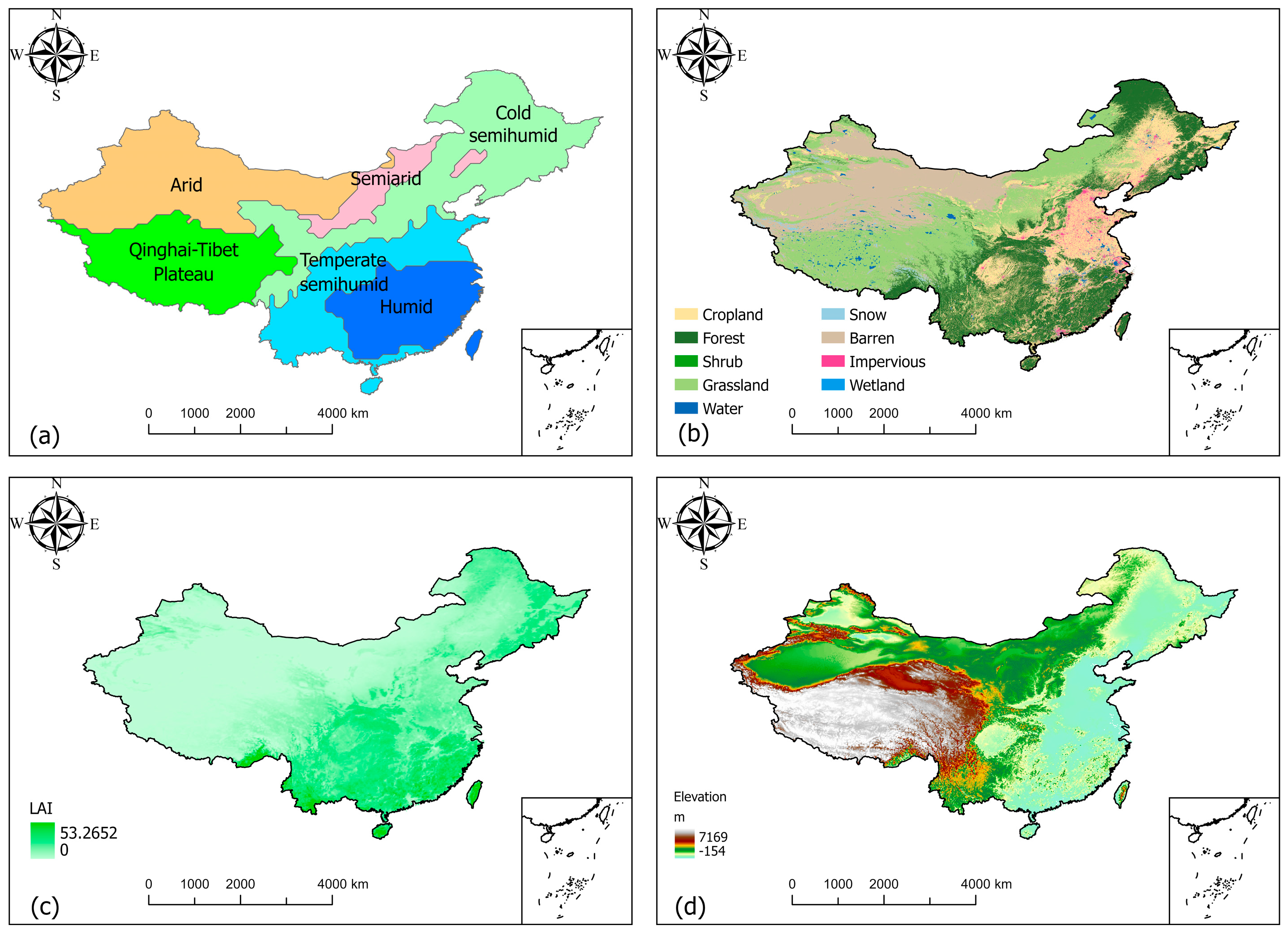
Mainland China is located in eastern Eurasia and covers approximately 9.6 million km², extending from 18° N to 54° N latitude and from 73° E to 135° E longitude (Figure 1). This broad geographic extent encompasses pronounced climatic, ecological, and topographic gradients, making China a suitable case for large-scale analyses of vegetation dynamics and environmental controls [21]. The country spans four major latitudinal zones, i.e., tropical, subtropical, temperate, and frigid, resulting in wide variation in hydrothermal conditions that strongly influence vegetation productivity and seasonality.

Regional climate patterns are dominated by the East Asian monsoon, producing a southeast–northwest decrease in precipitation and a south–north decrease in temperature. Southern regions experience warm, humid summers, whereas northern and inland areas are characterized by colder and drier conditions. Precipitation is highly uneven in both space and time, with more than 70% of annual rainfall occurring during the summer months, particularly in southern and eastern basins. These climatic contrasts contribute to strong spatial differentiation in vegetation types, biomass accumulation, and LAI dynamics [15,22].

To represent this spatial heterogeneity, we divided the study area into six climate zones based on thresholds of annual precipitation, mean temperature, and topographic structure, integrating national ecological zoning schemes with the Köppen-Geiger climate classification [14]. The resulting zones include: (1) Arid, (2) semi-arid, (3) cold semi-humid, (4) temperate semi-humid, (5) humid, and (6) the Qinghai-Tibet Plateau region. Each zone represents a distinct ecohydrological regime and dominant vegetation structure, ranging from desert shrubs and temperate grasslands to evergreen broadleaf forests and alpine tundra. This zonal framework enables comparative analysis of vegetation-climate relationships across environmental gradients and provides a consistent basis for assessing the relative influence of climatic, topographic, and anthropogenic factors on LAI dynamics.

2.2. Climate Zoning and Environmental Stratification

To represent this spatial heterogeneity, we divided the study area into six climate zones based on thresholds of annual precipitation, mean temperature, and topographic structure, integrating national ecological zoning schemes with the Köppen-Geiger climate classification [14]. The resulting zones include: (1) Arid, (2) semi-arid, (3) cold semi-humid, (4) temperate semi-humid, (5) humid, and (6) the Qinghai-Tibet Plateau region. Each zone represents a distinct ecohydrological regime and dominant vegetation structure, ranging from desert shrubs (dominated by xerophytic genera such as Artemisia spp., Haloxylon spp., and Calligonum spp.) and temperate grasslands (primarily Stipa spp. and Leymus spp.) to evergreen broadleaf forests (characterized by evergreen Fagaceae such as Castanopsis spp. and Lithocarpus spp.) and alpine tundra (dominated by alpine herbs and dwarf shrubs including Kobresia spp. and Carex spp.). This zonal framework enables comparative analysis of vegetation-climate relationships across environmental gradients and provides a consistent basis for assessing the relative influence of climatic, topographic, and anthropogenic factors on LAI dynamics.

When vegetation types are referenced in this study, representative genera or species are provided for clarification purposes only to indicate the dominant woody or herbaceous canopy components associated with each zone. These references are illustrative and do not imply exhaustive botanical classification or species-level analysis, which is beyond the large-scale, LAI-based structural focus of this study.

2.3. Data and Preprocessing

This study integrates multi-source vegetation, climatic, topographic, and anthropogenic datasets to examine long-term LAI dynamics across mainland China for the period 2000–2020. All datasets were reprojected to the WGS84 geographic coordinate system and resampled to a uniform spatial resolution of 0.1°, consistent with widely adopted practices in national- and continental-scale vegetation-climate analyses [8,23]. Continuous variables (e.g., temperature, precipitation, radiation) were resampled using bilinear interpolation, whereas categorical variables (e.g., land cover and fragmentation indicators) were resampled using nearest-neighbor assignment to preserve class integrity.

(1)

Vegetation datasets

LAI data were obtained from the GLASS V6 LAI product [23], which provides 8-day observations at 500 m spatial resolution. The GLASS product has been widely used in large-scale ecological studies due to its temporal continuity and noise-reduction procedures. To define forested areas consistently across datasets, annual maps from the China Land Cover Dataset (CLCD) were used to identify pixels classified as forest, which were then applied as a spatial mask for LAI analysis. Consequently, after spatial aggregation to the working resolution of 0.1°, LAI values represent the mean canopy condition of forested and other woody vegetation within each grid cell, potentially including mixtures of natural forests, plantations, secondary regrowth, and structurally similar woody covers. Accordingly, LAI is interpreted in this study as a continuous indicator of broad forest/woody canopy condition, rather than as a metric specific to individual forest types, species composition, stand age, or management regime. The modelling framework therefore diagnoses spatial variation in canopy density and structural expression, not ecosystem-specific or management-specific responses.

Monthly temperature and precipitation data were sourced from the Qinghai-Tibet Plateau Data Center [24]. These datasets provide spatially continuous and homogenized meteorological fields suitable for long-term vegetation-climate analyses. Downward shortwave radiation was obtained from [25], and soil moisture was derived from the multi-source fused soil moisture dataset developed by [26]. Climatic variables were aggregated to annual values to match the analytical framework.

(2)

Topographic factors

Elevation data were extracted from the Shuttle Radar Topography Mission (SRTM) digital elevation model, which provides near-global coverage at 90 m resolution [27]. Slope and aspect were derived from the Digital Elevation Model (DEM) to represent terrain-related constraints on vegetation distribution and growth. Elevation data were extracted from the Shuttle Radar Topography Mission (SRTM) digital elevation model. Slope and aspect were derived from the DEM using standard GIS procedures. Aspect represents slope orientation and is expressed in degrees from 0° to 360°, measured clockwise from north (0°/360° = north, 90° = east, 180° = south, 270° = west).

(3)

Anthropogenic indicators

Nighttime light data were obtained from the harmonized DMSP-OLS and VIIRS dataset [28] and used as a proxy for human activity intensity. Land cover information was extracted from the China Land Cover Dataset (CLCD) [29], which provides annual 30 m land cover maps. To accurately characterize landscape structural constraints, the Forest Fragmentation Index (FFI) was derived from the 30 m annual China Land Cover Dataset (CLCD). Specifically, forest pixels in the CLCD were extracted to generate a binary forest mask (forest = 1, non-forest = 0). Following the framework of Ma et al. (2023) [13], fragmentation-related landscape metrics were computed at the native 30 m resolution using a moving-window approach, with a window size of 5 km × 5 km centered on each pixel and treated as an individual landscape unit. Within each window, three landscape metrics were calculated: patch density (PD), edge density (ED), and a landscape connectivity metric (CONNECT). These metrics were min–max normalized to a common [0–1] scale and integrated using an equal-weight approach to derive the FFI, such that higher FFI values indicate higher forest fragmentation, characterized by patchier, edge-dominated forest patterns with reduced connectivity. For multi-source data harmonization, the resulting 30 m FFI layer was aggregated to the 0.1° analysis grid using the mean value within each grid cell. While the absolute magnitude of window-based fragmentation indices can vary with window size, the objective of this study is national-scale diagnosis; therefore, we expect the broad spatial patterns of fragmentation and their associations with LAI to remain robust at the reporting scale (0.1°).

(4)

Data harmonization

All datasets were temporally harmonized to annual resolution and spatially clipped using the national boundary of China. Only data from 2000–2020 were retained for analysis to ensure temporal consistency across variables.

Table 1. Datasets considered and used in this study.

Dataset	Spatial Resolution	Original Temporal Coverage	Units	Role in Analysis	Source
Leaf Area Index (GLASS V6)	500 m	2000–2024	m2 m−2	Used in final model	[23]
Precipitation	0.00833°	1901–2023	mm	Used in final model	[24]
Air temperature	0.00833°	1901–2023	°C	Used in final model	[24]
Downward shortwave radiation	0.1°	1951–2020	W m−2	Used in final model	[25]
Soil moisture	0.00833°	2000–2020	m3 m−3	Used in final model	[26]
Nighttime light intensity	0.1°	1992–2023	–	Used in final model	[28]
Digital Elevation Model (SRTM)	90 m	Static	m	Used in final model	[27]
Land cover (CLCD)	30 m	1985–2023	–	Used for derivation	[29]
Forest Fragmentation Index (FFI)	30 m (derived)	2000–2020	–	Used in final model	[17]
Soil organic carbon	1 km	1985–2020	kg C m−2	Screened, excluded (VIF)	[30]
Wind speed	0.1°	1980–2022	m s−1	Screened, excluded (VIF)	[31]
Surface pressure	0.1°	1980–2022	hPa	Screened, excluded (VIF)	[31]
Relative humidity	0.1°	1980–2022	%	Screened, excluded (VIF)	[31]
Climate zones (Köppen-Geiger)	–	Static	–	Stratification variable	[14]

Note: All datasets were harmonized to a common spatial resolution of 0.1° and restricted to the overlapping period 2000–2020 for analysis. Variables excluded due to multicollinearity were identified using variance inflation factor screening (Section 3.1).

summarizes the datasets used, including spatial resolution, temporal coverage, and sources.

2.4. Methods

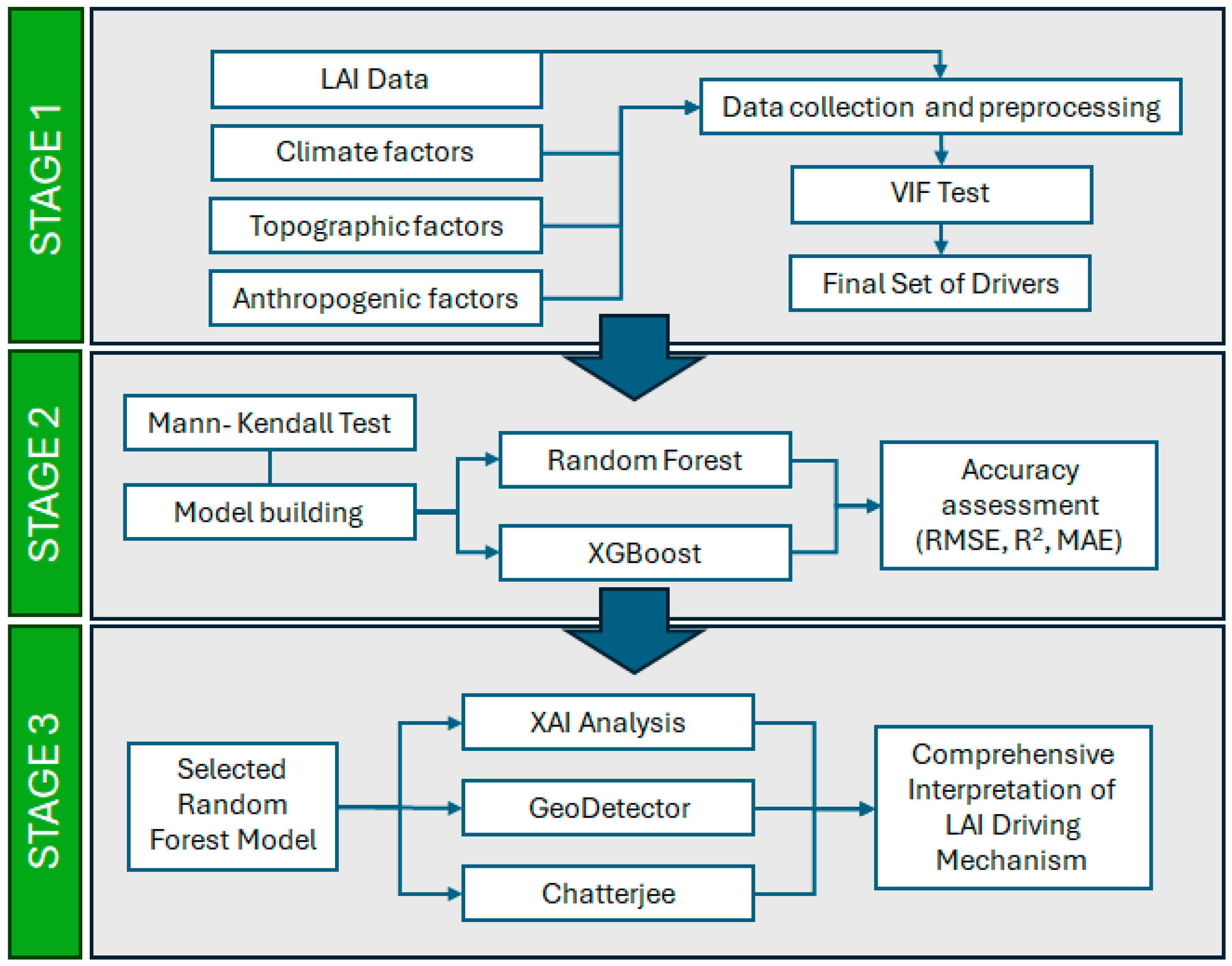
The analytical framework integrates machine-learning modeling, model interpretability techniques, and spatial statistical diagnostics to characterize the relative influence and spatial heterogeneity of climatic, topographic, and anthropogenic factors associated with LAI dynamics across China. The framework comprises four sequential components. First, a machine-learning model is constructed to capture nonlinear relationships between LAI and relevant environmental variables. Second, SHapley Additive exPlanations (SHAP) [9] are applied to interpret model behavior by quantifying the relative contribution and direction of individual predictors. Third, the Chatterjee correlation coefficient [12] is used to assess univariate nonlinear dependence between LAI and candidate drivers, providing a complementary statistical perspective independent of the machine-learning model. Additionally, the spatial stratified heterogeneity and interaction effects are evaluated using the GeoDetector method [10,11], a spatial statistical approach for detecting stratified heterogeneity and factor interactions. Together, these components provide a transparent and spatially explicit diagnostic framework for examining vegetation–environment relationships across heterogeneous landscapes (Figure 2).

2.4.1. LAI Preprocessing and National Averaging

Annual LAI data were derived from the GLASS LAI product at 500 m spatial resolution. Annual LAI rasters were first clipped to the mainland China boundary using a national polygon mask, such that pixels outside the study domain were excluded. The clipped LAI data were then spatially aggregated to a working resolution of 0.1° using bilinear interpolation to ensure consistency with the resolution of the predictor datasets. National-scale mean LAI was calculated as the spatial mean of the aggregated 0.1° LAI grids. Grid cells within the China domain lacking valid LAI retrievals were assigned a value of zero, such that the resulting mean reflects both vegetation presence and canopy density across the full mainland China area, rather than a conditional mean over vegetated pixels only. This definition was applied consistently across all years to ensure comparability of national-scale LAI trends.

2.4.2. Predictor Selection and Spatiotemporal Changes

Multicollinearity was assessed using the Variance Inflation Factor (VIF) to exclude redundant predictors and enhance results interpretability [32].

The trend in mean annual LAI and the selected predictors was quantified using the Theil-Sen median slope estimator [33,34], a robust non-parametric method that effectively handles outliers and non-normal data distributions [35]. Trend significance was assessed with the Mann–Kendall test [36], which is similarly insensitive to outliers and makes no assumptions about the underlying distribution. Both analyses were implemented in Python using the SciPy library.

2.4.3. Machine-Learning Modelling of LAI-Environment Relationships

To characterize nonlinear associations between LAI and environmental variables, machine-learning models were implemented in Python (version 3.9.18). LAI and predictor raster layers were processed using the rasterio library, converted to numerical arrays, and combined into a feature matrix after removing grid cells with missing values.

Two ensemble learning algorithms were evaluated: Random forest (RF) [37] and extreme gradient boosting (XGBoost) [38]. The RF model was implemented using the RandomForestRegressor function in scikit-learn, with 1500 trees and parallel computation enabled (n_jobs = −1). XGBoost was implemented using the xgboost Python package with 1500 estimators, a maximum tree depth of 6, a learning rate of 0.05, and GPU-accelerated tree construction (tree_method = “gpu_hist”).

The dataset was randomly divided into training (80%) and validation (20%) subsets. Model performance was evaluated using 10-fold cross-validation and independent validation based on the coefficient of determination (R²), root mean square error (RMSE), and mean absolute error (MAE). Given the spatially structured nature of gridded environmental data, model evaluation is interpreted as diagnostic of spatial associations rather than predictive performance. Feature importance metrics from both models (Gini importance for RF and gain-based importance for XGBoost) were used as preliminary indicators prior to model interpretation.

To evaluate model performance, the dataset was randomly divided into training (80%) and validation (20%) subsets. This evaluation strategy was adopted because the objective of the modeling step is spatial diagnosis rather than spatial prediction, and model performance metrics are therefore interpreted as measures of spatial association rather than as indicators of predictive skill for independent locations. Given the strong spatial autocorrelation inherent in gridded environmental datasets, we acknowledge that random sampling may lead to inflated coefficients of determination (R²). However, performance statistics are used here solely to confirm the model’s ability to capture dominant spatial structure prior to interpretation, not to assess generalization performance across independent spatial units.

2.4.4. Model Interpretation Using SHAP Values

Although ensemble learning models can capture complex nonlinear relationships, their internal decision processes are not directly interpretable. To improve transparency, the SHapley Additive exPlanations (SHAP) framework was applied to decompose model outputs into additive contributions from individual predictors [6,9]. SHAP analysis was used to support: (i) global interpretation, by ranking predictors according to their overall contribution; (ii) local interpretation, by examining spatial variation in predictor influence across different regions; and (iii) nonlinear response characterization, by identifying threshold behaviour and interaction patterns. This approach enables an interpretable and model-agnostic assessment of how individual variables contribute to spatial variation in LAI.

2.4.5. Nonlinear Association Assessment Using the Chatterjee Correlation Coefficient

To complement model-based interpretation, the Chatterjee correlation coefficient [12] (ξ) was calculated to assess nonlinear dependence between LAI and individual predictor variables. Unlike traditional correlation measures (e.g., Pearson or Spearman), ξ captures arbitrary forms of dependence without assuming linearity or monotonic rank correspondence. The coefficient ranges from 0, indicating statistical independence, to 1, indicating perfect functional dependence. This analysis provides an independent, distribution-free measure of association that is not tied to the machine-learning model structure.

Spatial Heterogeneity Assessment Using GeoDetector

Because environmental controls on LAI may vary across space, spatial stratified heterogeneity was assessed using the GeoDetector method [10,11]. GeoDetector quantifies the extent to which the spatial distribution of a factor corresponds to the spatial stratification of a response variable using the q-statistic (Equation (1)). Higher q values indicate stronger spatial correspondence between a factor and LAI.

$$q=1-{\displaystyle \frac{{\displaystyle \sum _{h=1}^L{N}_h}{\sigma }_h^2}{N{\sigma }^2}}$$

(1)

where $N_h$ and ${\sigma }_h^2$ denote the sample size and variance within stratum h, and N and ${\sigma }^2$ represent the total sample size and variance. A higher q value indicates stronger explanatory power.

In addition to evaluating individual factors, GeoDetector was used to examine pairwise interaction effects, allowing assessment of whether combined factors enhance or weaken spatial stratification relative to their individual effects. This analysis supports the identification of regionally differentiated control regimes across heterogeneous environmental conditions.

3. Results

3.1. Predictor Selection and Multicollinearity Assessment

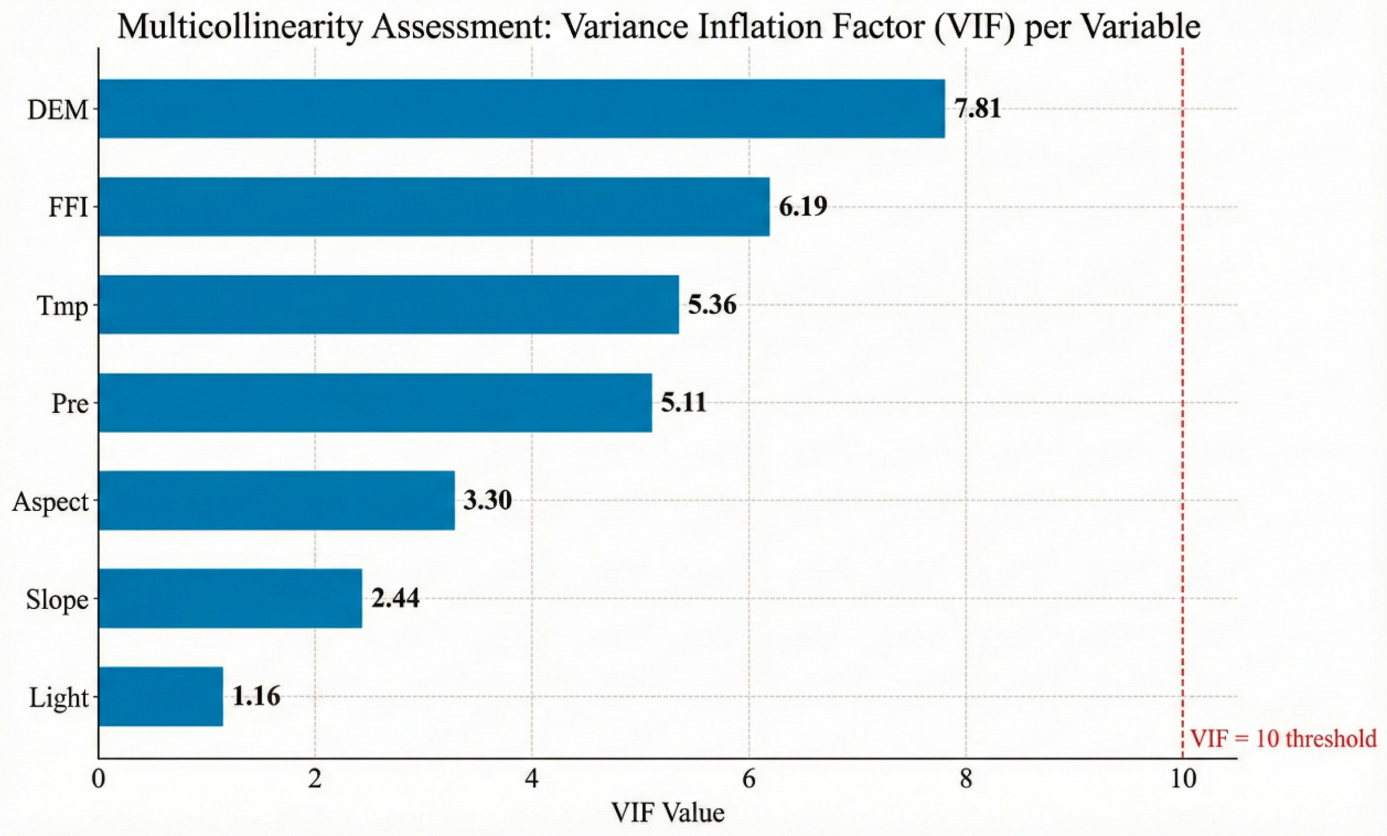
To reduce the influence of multicollinearity among candidate predictors, variance inflation factor (VIF) screening was conducted prior to model development. All climatic, topographic, and anthropogenic variables listed in Table 1 were initially considered. Variables with VIF values exceeding the commonly used threshold of 10 were excluded to improve numerical stability and facilitate model interpretation.

Following VIF screening, seven variables were retained for subsequent analysis: air temperature, precipitation, downward shortwave radiation, soil moisture, nighttime light intensity, elevation, and the FFI (Figure A1). All retained variables exhibited VIF values well below the threshold, indicating acceptable levels of collinearity and minimizing redundancy among predictors. This selection ensured that the remaining variables capture complementary aspects of the environmental conditions associated with spatial variation in LAI.

3.2. Spatiotemporal Patterns of LAI and Associated Environmental Variables

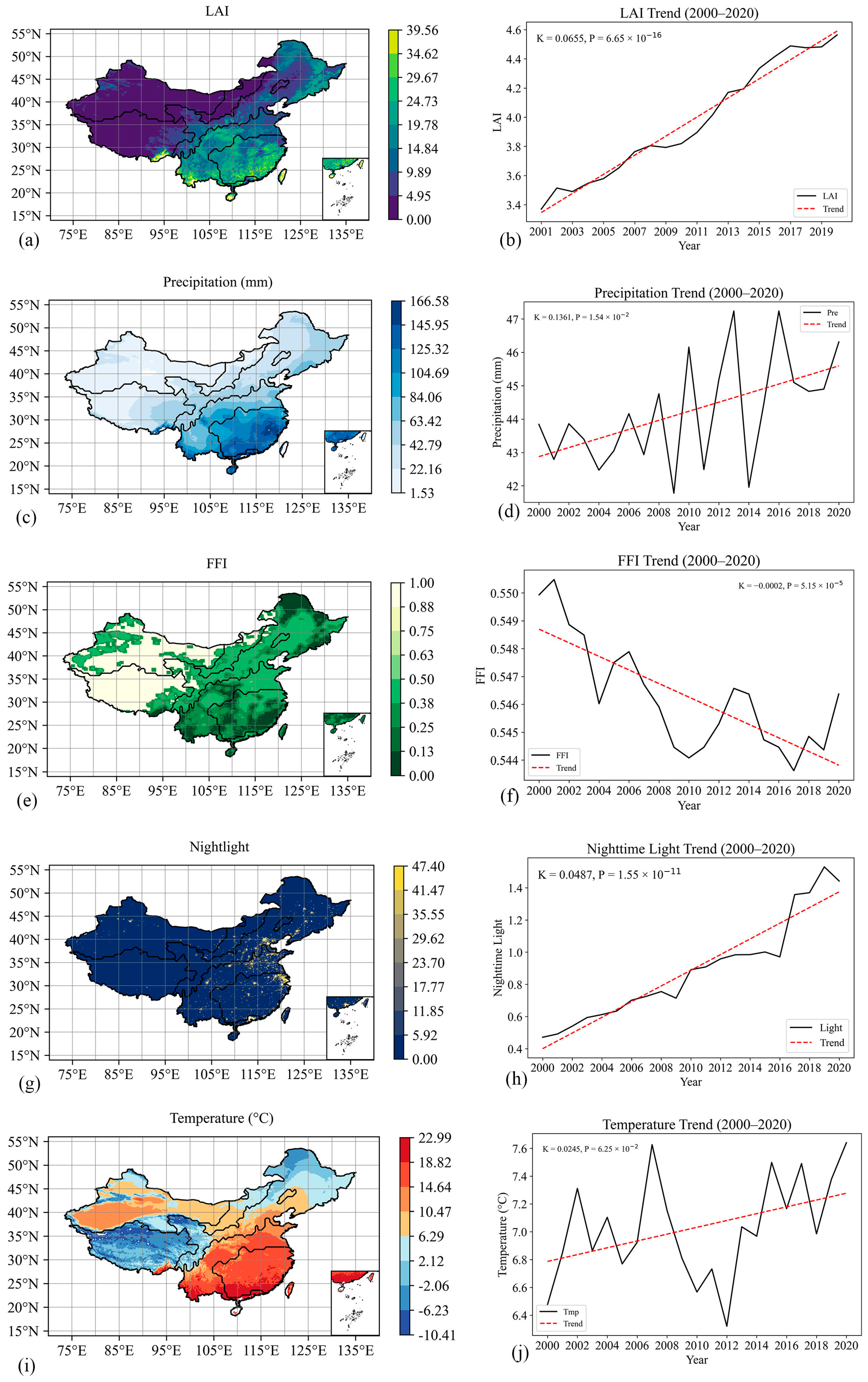
Figure 3 summarizes the spatial distributions and temporal trends of LAI and key environmental variables across mainland China during 2000–2020. LAI exhibits a wide-spread increasing tendency across most vegetated regions. LAI shows strong heterogeneity, with higher values mainly concentrated in the humid and densely vegetated regions of southern and eastern China, where woody canopies are typically dominated by evergreen and mixed broadleaf taxa (e.g., Castanopsis spp., Schima spp., Cyclobalanopsis spp.), while lower values occur in northwestern China and the Qinghai-Tibet Plateau.

Precipitation displays a pronounced southeast-northwest gradient, with substantially higher annual totals in southeastern China (Figure 3c). Interannual precipitation shows a modest upward tendency over the study period (Figure 3d), accompanied by considerable year-to-year variability. Regional contrasts are evident, with increasing precipitation in southern China and relatively stable or weakly declining trends in parts of northern regions.

The FFI shows a general decreasing pattern nationwide (Figure 3e), with lower fragmentation values concentrated in mountainous regions of southwestern and northeastern China. The temporal evolution of FFI indicates a gradual decline over the study period (Figure 3f), reflecting an overall tendency toward increased forest structural continuity at the national scale.

Nighttime light intensity increased markedly across China between 2000 and 2020 (Figure 3g,h), with particularly strong growth in major urban agglomerations such as the North China Plain, Yangtze River Delta, and Pearl River Delta. This trend reflects the rapid expansion and intensification of human activities during the study period.

Mean air temperature exhibits clear spatial differentiation, with lower values in high-elevation regions such as the Qinghai-Tibet Plateau and higher values in lowland areas (Figure 3i). From 2000 to 2020, temperature increased steadily across most regions (Figure 3j), with a total rise of approximately 0.6–0.8 °C, consistent with observed warming trends across East Asia.

Together, these patterns highlight substantial spatial and temporal heterogeneity in both LAI and its associated environmental variables, providing the contextual basis for subsequent analyses of nonlinear associations, interaction effects, and spatially differentiated control regimes.

3.3. Model Performance and Selection

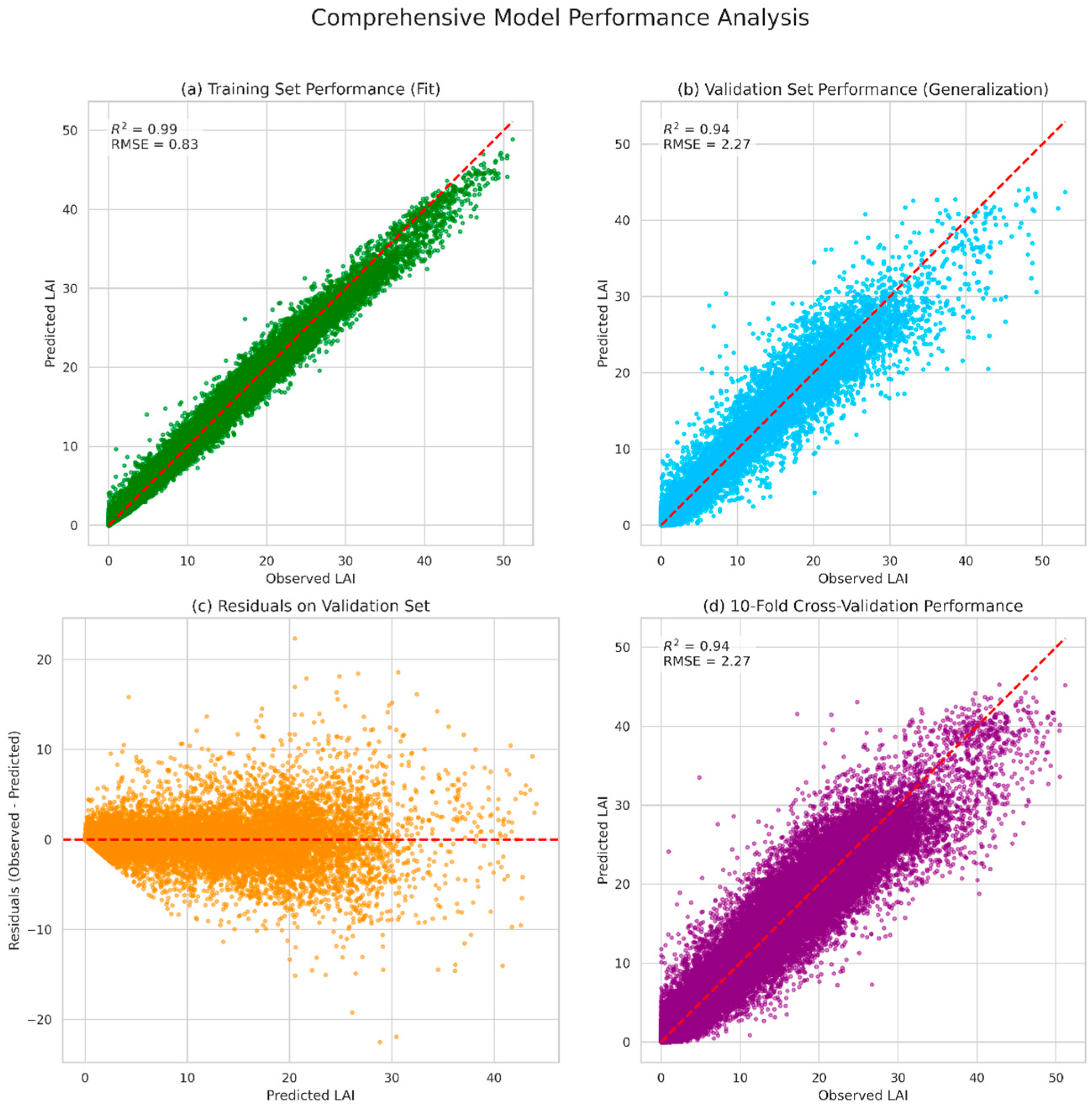
Both Random Forest (RF) and XGBoost models exhibited strong ability to reproduce observed spatial patterns of LAI across China. Overall, the RF model outperformed XGBoost and was therefore retained for subsequent interpretation. Using 10-fold cross-validation, the RF model achieved a mean coefficient of determination (R² = 0.94), with a root mean square error (RMSE = 2.27) and mean absolute error (MAE = 1.32). XGBoost yielded slightly lower performance metrics but showed similar variable ranking patterns. On the independent 20% hold-out dataset, the RF model produced performance metrics comparable to those obtained from cross-validation (R² = 0.94, RMSE = 2.27, MAE = 1.32). Training and test R² were nearly identical, consistent with strong spatial patterns and RF’s resistance to overfitting. Given the spatially structured nature of the input data, these metrics are interpreted as reflecting the model’s ability to capture dominant spatial associations rather than as indicators of predictive performance for independent spatial locations. The close agreement between cross-validation and hold-out results suggests stable model behavior under the chosen diagnostic framework. Given the strong spatial autocorrelation inherent in gridded environmental datasets, model performance metrics are interpreted as measures of spatial association rather than predictive accuracy for independent locations.

As illustrated in Figure A2a,b, predicted and observed LAI values align closely along the 1:1 line for both training and validation datasets. Residuals are symmetrically distributed around zero (Figure A2c), with no evident systematic bias across the range of predictions. Cross-validation results (Figure A2d) are consistent with independent validation, supporting the robustness of the model for subsequent interpretability analyses.

3.4. Drivers’ Relative Contributions and Response Patterns

3.4.1. SHAP-Based Feature Importance

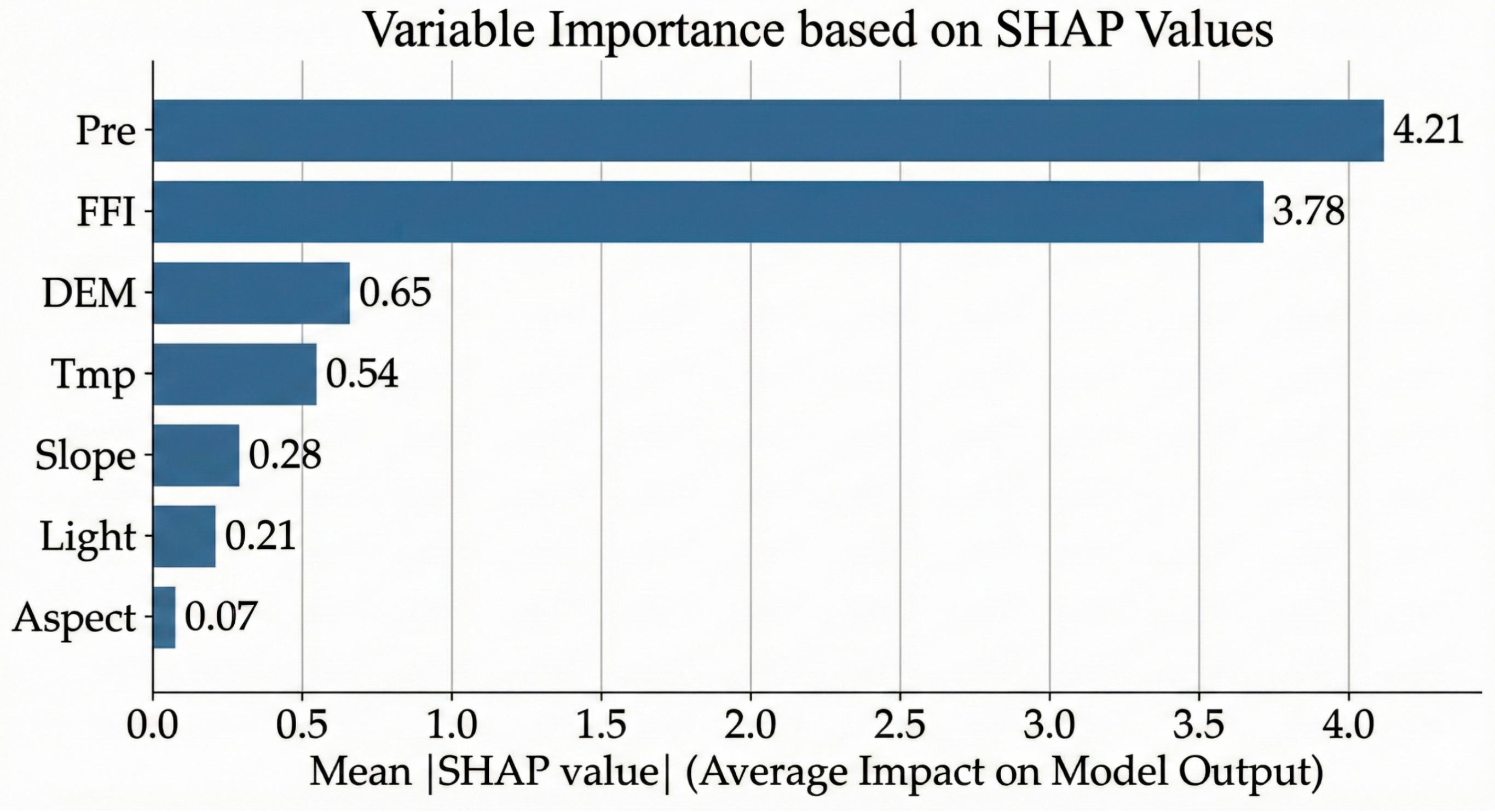
Figure 4 summarizes the relative importance of environmental variables based on mean absolute SHAP values. Among all predictors, precipitation shows the largest contribution to spatial variation in LAI at the national scale. The FFI ranks second, indicating that landscape structural characteristics are strongly associated with observed differences in LAI. Elevation and air temperature exhibit moderate contributions, while slope, nighttime light intensity, and aspect display comparatively smaller SHAP values, suggesting weaker overall associations with LAI at the national scale.

The separation in SHAP magnitudes highlights pronounced differences in the relative influence of climatic, topographic, and anthropogenic variables, providing a basis for subsequent analyses of nonlinear response behavior and spatial heterogeneity.

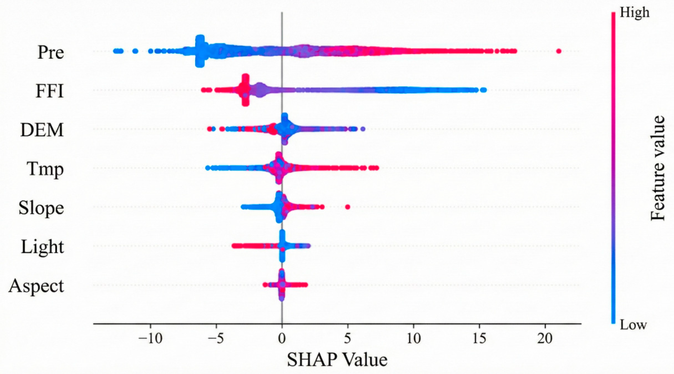
Figure A3 presents the distribution of SHAP values for individual predictors, illustrating both the magnitude and direction of their contributions across all grid cells. Precipitation exhibits the widest SHAP range, reflecting strong variability in its association with LAI across contrasting environmental conditions. Higher precipitation values are generally associated with positive SHAP contributions, whereas lower values correspond to reduced LAI. The forest fragmentation index also shows a broad SHAP distribution, with higher fragmentation values predominantly associated with negative contributions to LAI and lower fragmentation linked to positive contributions.

Elevation and temperature display more moderate and condition-dependent SHAP patterns, indicating spatially variable associations across different environmental contexts. In contrast, slope, nighttime light intensity, and aspect exhibit narrow SHAP ranges centered near zero, suggesting limited and relatively uniform influence at the national scale. Together, these SHAP-based results provide pixel-level evidence that complements the aggregated importance rankings and supports subsequent investigation of interaction effects and spatial differentiation.

3.4.2. Nonlinear Univariate Response Patterns

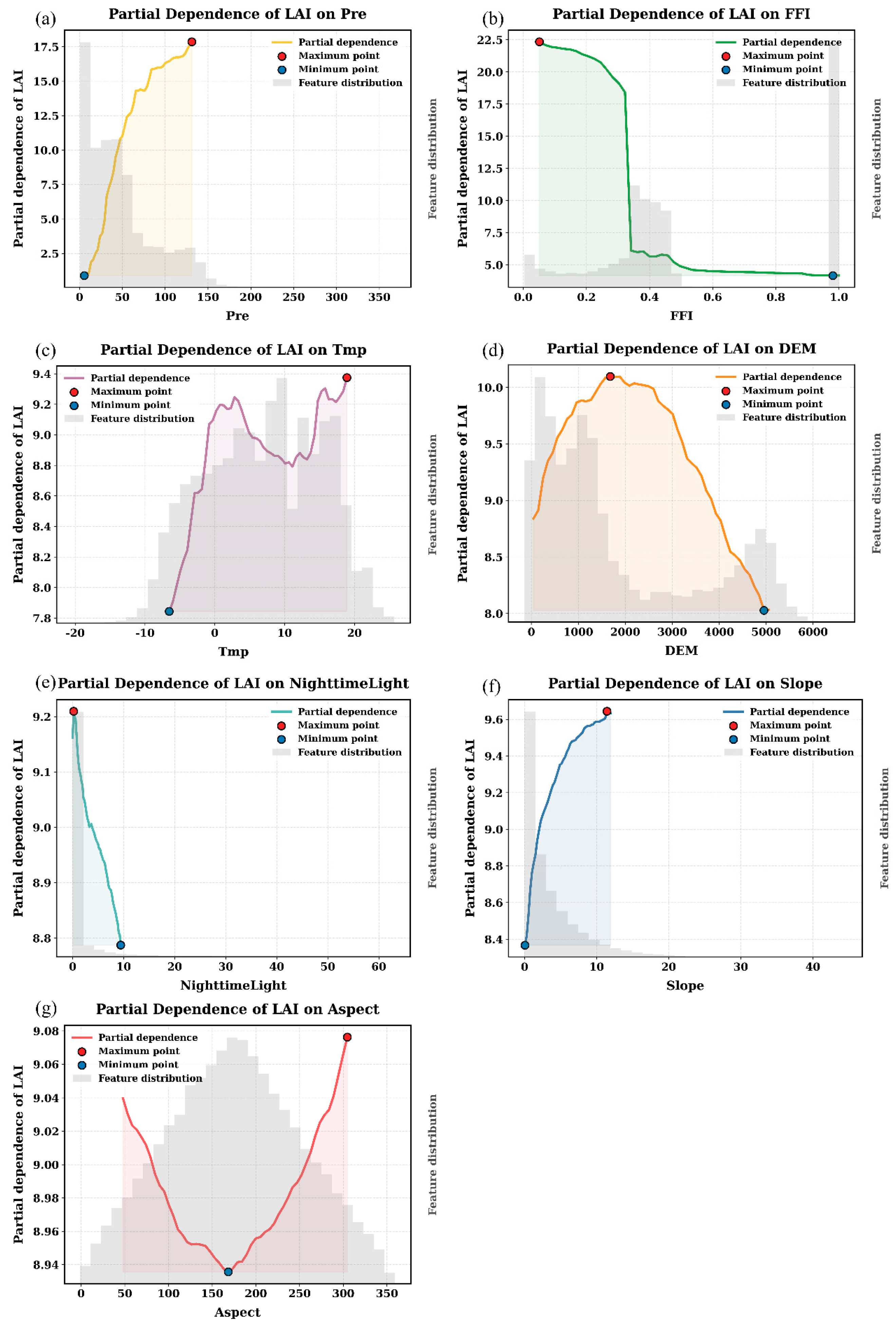
Figure A4 illustrates the nonlinear response patterns of LAI to individual predictor variables based on partial dependence analysis. These curves describe the marginal association between each variable and modeled LAI while averaging the effects of other predictors.

Precipitation exhibits a strong positive association with LAI, characterized by a rapid increase at low precipitation levels followed by a gradual saturation beyond approximately 120–150 mm (Figure A4a). This pattern indicates diminishing marginal gains in LAI under higher moisture conditions. The FFI shows a clear monotonic negative association with LAI (Figure A4b). LAI declines sharply as FFI increases from low values up to approximately 0.3, after which the rate of decline becomes more gradual, suggesting heightened sensitivity to early stages of fragmentation.

Air temperature displays a nonlinear and non-monotonic association with LAI (Figure A4c), with alternating increases and decreases across the temperature range, reflecting spatial aggregation of contrasting thermal environments. Elevation exhibits a hump-shaped response (Figure A4d), with LAI increasing from low to mid elevations (approximately 2000–3000 m) before declining at higher elevations, consistent with increasing thermal and environmental constraints.

Nighttime light intensity shows a predominantly negative association with LAI (Figure A4e), with pronounced reductions at lower light levels followed by a plateau. Slope exhibits a positive but saturating pattern, with LAI increasing up to slopes of approximately 10° and remaining relatively stable thereafter (Figure A4f). Aspect displays the weakest response (Figure A4g), with minor variation across orientations and limited overall influence on LAI magnitude.

Together, these partial dependence patterns highlight pronounced nonlinearity and heterogeneity in the associations between LAI and climatic, topographic, and anthropogenic variables, complementing the SHAP-based importance rankings and supporting subsequent interaction analyses.

3.5. Interaction Patterns and Moisture-Fragmentation Coupling

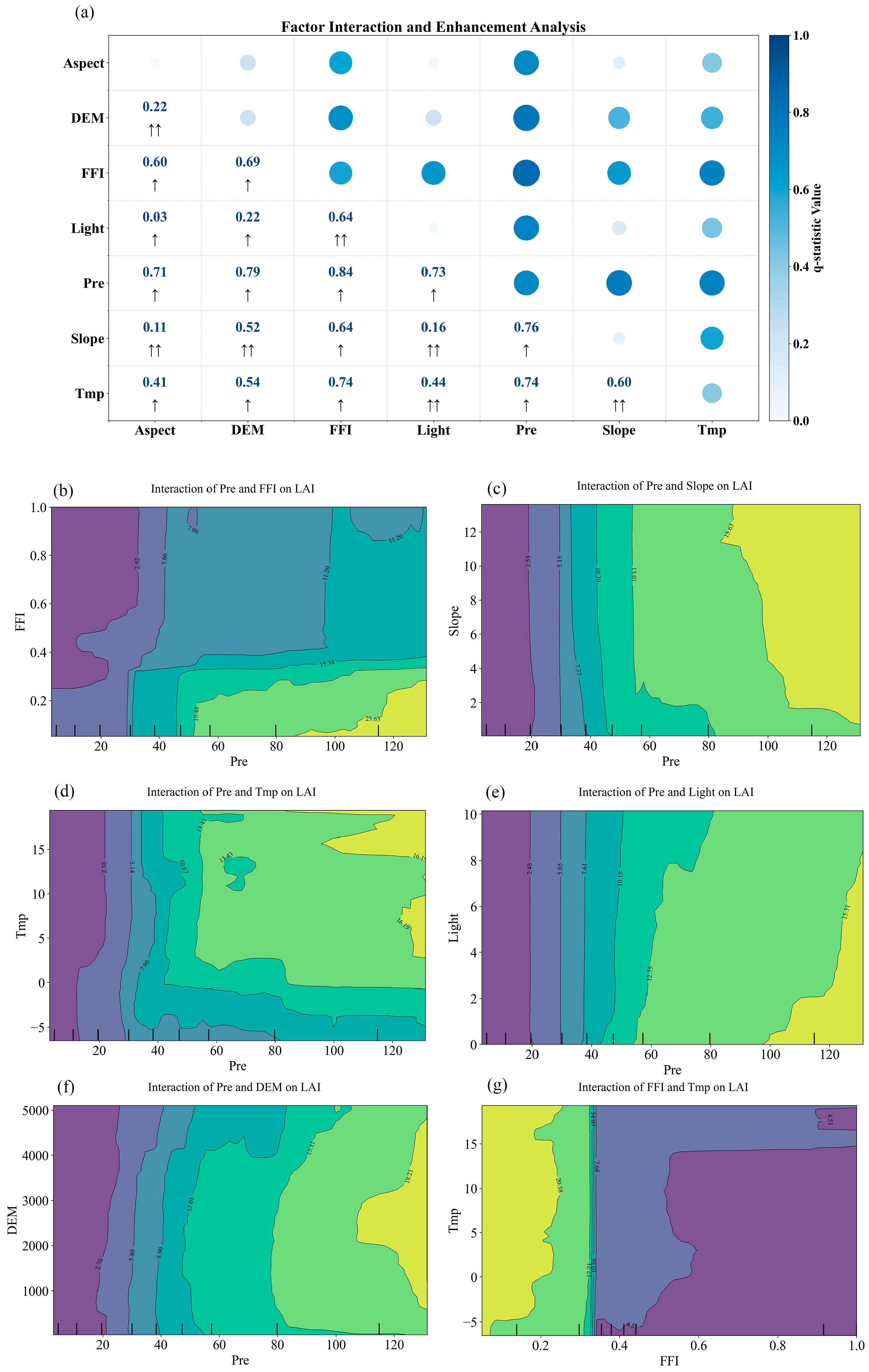
GeoDetector interaction analysis and bivariate partial dependence plots (2D-PDPs) indicate that spatial variation in LAI is characterized by pronounced non-additive interaction patterns among environmental variables rather than by independent effects alone (Figure 5). In most cases, interaction q-statistics exceed those of individual variables, highlighting the importance of combined influences in shaping spatial LAI patterns.

The strongest interaction is observed between precipitation and the FFI, providing a diagnostic representation of a moisture-fragmentation coupling pattern (Figure 5a,b). The 2D-PDP shows that the positive association between precipitation and LAI is more pronounced under low fragmentation conditions, whereas this association weakens substantially as fragmentation increases. Under highly fragmented landscapes, increases in precipitation are associated with comparatively smaller gains in modeled LAI, indicating that landscape structure modulates the strength of climate-LAI associations. This interaction pattern suggests that fragmentation constrains the extent to which vegetation structure responds to moisture availability, particularly in water-limited environments.

Interactions involving topographic factors further highlight spatial modulation of environmental associations. The interaction between elevation and temperature (Figure 5c) indicates that temperature–LAI relationships vary systematically with altitude, with positive associations at low to mid elevations and weaker or saturated responses at high elevations, such as on the Qinghai-Tibet Plateau. Similarly, the interaction between FFI and elevation suggests that fragmentation effects are strongest in lowland regions, while higher elevations exhibit weaker fragmentation–LAI associations, potentially reflecting reduced accessibility and human disturbance.

An additional interaction between precipitation and nighttime light intensity (Figure 5d) indicates that areas with higher human activity exhibit reduced sensitivity of LAI to precipitation variability. This pattern is consistent with the notion that anthropogenic modification of land surfaces may alter vegetation-water relationships, although the specific processes involved cannot be resolved within the present analytical framework.

Overall, these interaction patterns demonstrate that landscape structure and topography systematically modulate the spatial associations between climate variables and LAI. Rather than acting independently, climatic and anthropogenic factors interact in ways that produce regionally differentiated LAI responses, underscoring the importance of considering combined effects when diagnosing vegetation dynamics across heterogeneous landscapes.

3.6. Spatial Divergence of Dominant Association Patterns

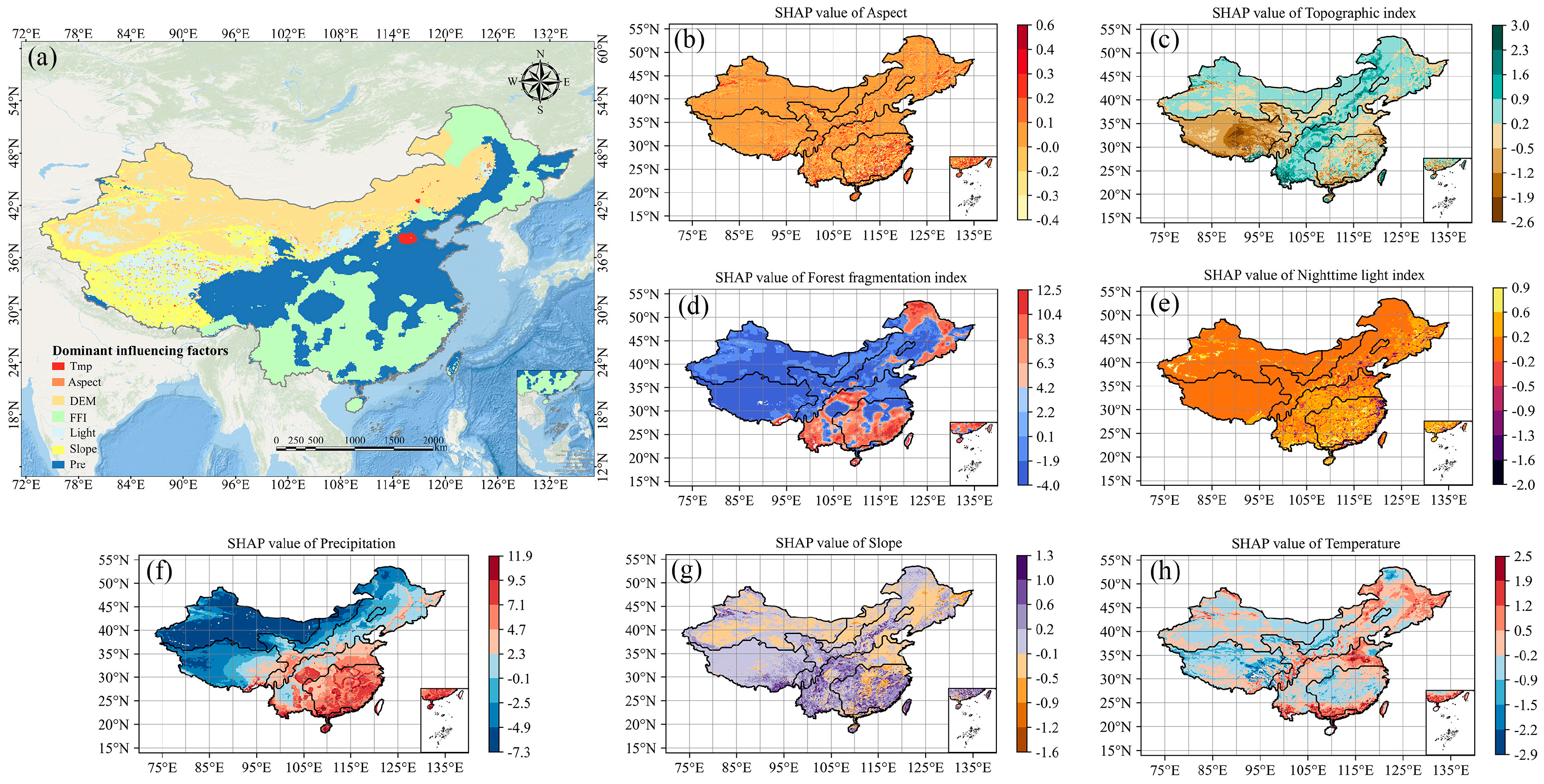
Spatially explicit SHAP results (Figure 6) and nonlinear dependence analysis using the Chatterjee coefficient (Figure A5) reveal pronounced regional differentiation in the dominant environmental associations with LAI acro iss China. These patterns indicate systematic shifts in the relative importance of climatic, topographic, and anthropogenic variables across contrasting environmental contexts.

3.6.1. Precipitation-Dominated Associations in Humid Regions

In humid and temperate semi-humid zones, including the Yangtze River Basin and southern China, where woody canopies are predominantly composed of evergreen and mixed broadleaf taxa such as Castanopsis spp., Schima spp., and Cyclobalanopsis spp., precipitation consistently exhibits the strongest association with LAI.

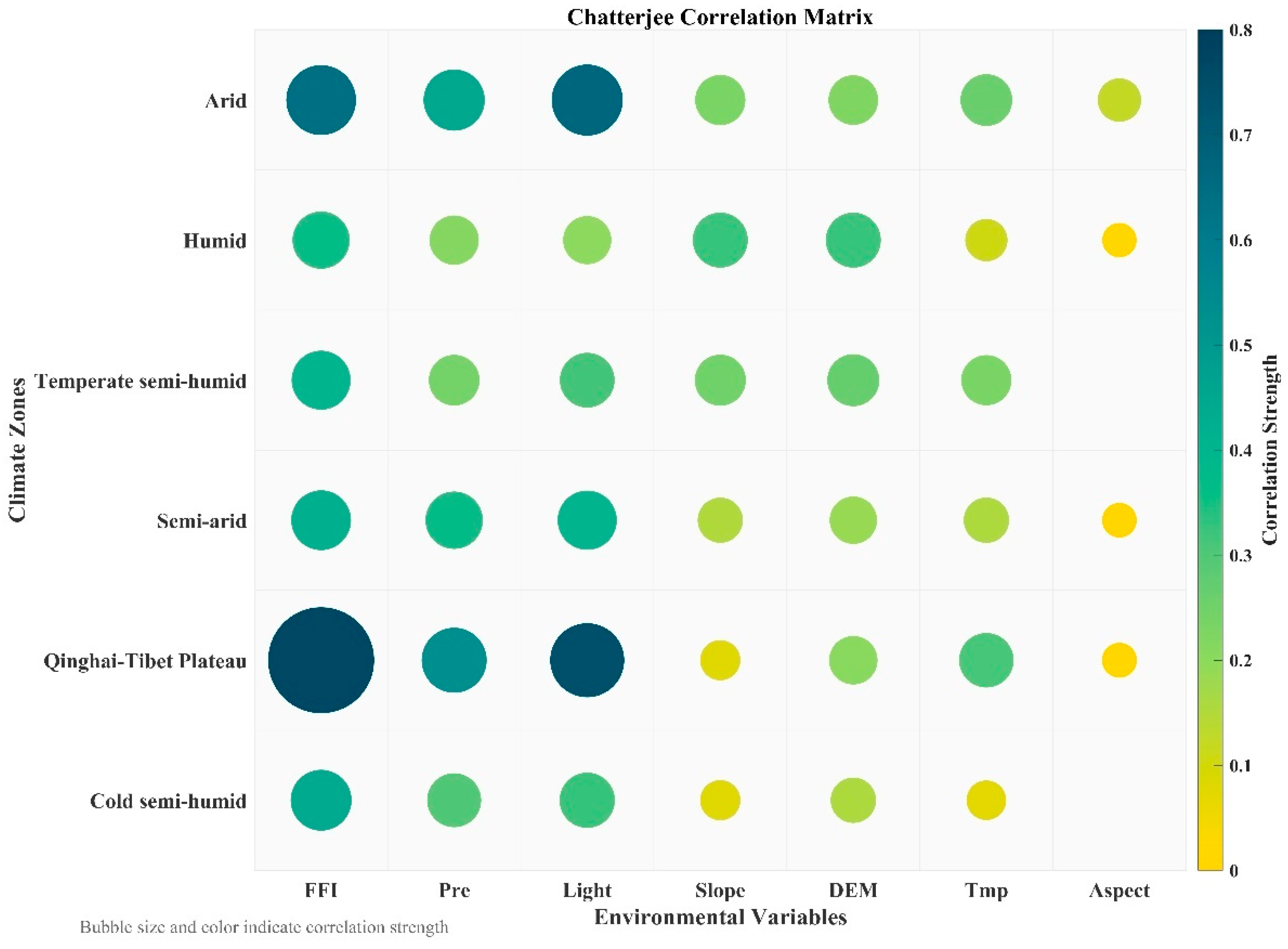
Spatial SHAP maps (Figure 6f) show high positive precipitation-related contributions concentrated in southeastern monsoon-influenced regions, with a gradual decrease toward northwestern China. This spatial gradient broadly corresponds to known hydroclimatic transitions across China. Chatterjee coefficients further indicate strong precipitation–LAI dependence in humid zones (Figure A5), suggesting that moisture availability is a primary correlate of spatial LAI variation where energy limitations are relatively weak.

3.6.2. Fragmentation-Associated Patterns in Arid and Semi-Arid Regions

In arid and semi-arid regions of northwestern China and Inner Mongolia, where woody vegetation is sparse and typically dominated by drought-adapted shrubs (e.g., Artemisia spp., Haloxylon spp.), the FFI exhibits stronger associations with LAI than climatic variables. The dominant-factor map (Figure 6a) highlights extensive areas where FFI represents the largest contributor in SHAP magnitude terms. Spatial SHAP patterns for FFI (Figure 6d) show predominantly negative contributions in these regions, indicating that higher fragmentation is associated with lower LAI. Chatterjee coefficients corroborate this pattern, with FFI showing the highest univariate dependence with LAI in dryland zones (Figure A5). Together, these results indicate that landscape structure is a key correlate of spatial LAI variability in water-limited environments.

3.6.3. Topographic and Thermal Associations on the Qinghai-Tibet Plateau

On the Qinghai-Tibet Plateau, elevation and temperature exhibit strong spatial associations with LAI. SHAP maps for elevation and temperature (Figure 6c,h) show distinct clustering over the Plateau, reflecting the dominant role of topographic and thermal gradients. Temperature-related SHAP values are positive in lower-elevation valleys but diminish or reverse at higher elevations, consistent with strong altitudinal constraints. Chatterjee coefficients also indicate notable associations between LAI and anthropogenic proxies, such as nighttime light intensity, suggesting localized human influences within an otherwise topographically constrained environment.

3.6.4. Spatial Signatures of Anthropogenic Activity

Nighttime light intensity shows localized associations with LAI, particularly in major urban agglomerations such as the Pearl River Delta and Yangtze River Delta (Figure 6e). In addition, relatively high nighttime light–LAI dependence is observed in arid and plateau regions (Figure A5), likely reflecting the spatial concentration of vegetation in human-managed landscapes such as oases and valley settlements. These patterns indicate that human activity is spatially co-located with higher LAI in environmentally constrained regions, although the underlying processes cannot be resolved from the present analysis.

Overall, these results demonstrate that the spatial associations between LAI and environmental variables vary systematically across climatic and physiographic contexts. Rather than a uniform national pattern, LAI exhibits regionally differentiated association structures that reflect combined influences of climate, landscape structure, topography, and human activity.

4. Discussion

4.1. Interpretable Diagnostics of Large-Scale LAI Variability

This study applies an interpretable, nationally scalable analytical framework to diagnose how climatic, topographic, and landscape-structural factors are associated with large-scale variation in LAI across China, with explicit relevance for spatial environmental assessment and regionally differentiated interpretation of vegetation patterns. By integrating SHAP-based explainable artificial intelligence, GeoDetector interaction analysis, and Chatterjee nonlinear dependence assessment, the framework moves beyond conventional black-box modeling and enables transparent examination of how climatic, topographic, and anthropogenic variables are associated with spatial variation in vegetation structure. This approach responds to recent calls for interpretable and theory-informed applications of machine learning in Earth system science [8,39] and demonstrates how predictive models can be repurposed for ecological diagnosis rather than forecasting alone.

At the national scale, mean LAI increased substantially over the study period, rising from approximately 3.4 to 4.6, consistent with previously reported large-scale greening signals based on satellite observations [4] and long-term MODIS-based LAI assessments [23]. The consistency in the direction and persistence of the greening signal across independent data products supports the robustness of the input datasets and modeling framework, while reinforcing that the observed LAI increase reflects broad-scale vegetation changes rather than model artifacts. The relatively high absolute values reflect the fact that the national mean LAI is computed over the mainland China domain at 0.1° resolution and incorporates both vegetation presence and canopy density across extensive forested and intensively managed landscapes, rather than representing a global land average or a conditional forest-only metric.

4.2. Climatic Controls and Nonlinear Saturation Effects

The results reveal pronounced nonlinearity and spatial heterogeneity in the associations between LAI and environmental variables. Precipitation consistently exhibits the strongest association with LAI, but partial dependence analysis indicates a clear saturation pattern under humid conditions. This behavior is consistent with ecohydrological theory, suggesting diminishing vegetation responses once moisture availability exceeds limiting thresholds in monsoonal regions [40]. Importantly, these patterns should be interpreted as spatial associations rather than physiological response functions, reflecting aggregated behavior across diverse ecosystems and climate regimes.

4.3. Landscape Structure as a Climate-Conditioned Constraint

A notable finding is the consistently high importance of the FFI, which ranks second nationally and exhibits particularly strong associations with LAI in arid and semi-arid regions. Unlike classical landscape ecological frameworks that emphasize threshold responses to fragmentation [41], the SHAP and partial dependence results indicate a largely monotonic negative association between fragmentation and LAI. This pattern is especially pronounced in dryland environments, where GeoDetector and Chatterjee analyses show that landscape structure explains spatial variation in LAI as strongly as, or more strongly than, climatic variables. These results are consistent with recent evidence that fragmentation can exacerbate environmental stress in drylands by altering microclimate, connectivity, and resource redistribution [42,43]. However, the present analysis does not resolve causal pathways, and such mechanisms should be regarded as plausible interpretations rather than demonstrated processes.

4.4. Interaction Effects and Spatially Differentiated Control Regimes

The strong interaction between precipitation and fragmentation further suggests that landscape structure modulates how climatic variability is expressed in vegetation structure, particularly in water-limited systems. In fragmented drylands, increased edge-to-core ratios can expose vegetation to harsher microclimatic conditions, including elevated wind speeds, higher vapor pressure deficits, and greater temperature variability, which accelerate soil moisture loss and reduce the efficiency with which precipitation inputs are translated into canopy development [44,45]. Fragmentation may also disrupt ecological connectivity, constraining seed dispersal, root network continuity, and belowground water redistribution across patches [46]. In such contexts, additional rainfall may yield comparatively smaller increases in LAI, consistent with the suppressed precipitation sensitivity observed in highly fragmented regions [42,47]. While these mechanisms cannot be isolated directly within the present framework, they provide a coherent ecological interpretation of the observed moisture-fragmentation coupling.

Anthropogenic influence, as proxied by nighttime light intensity, shows more localized and context-dependent associations with LAI. While nighttime lights are widely used as indicators of urbanization and human activity [48], their relatively modest contribution at the national scale suggests limitations in capturing structural landscape processes relevant to vegetation dynamics. In contrast, fragmentation metrics appear more sensitive to changes associated with forest recovery and reorganization, such as those reported for regions affected by the Grain-for-Green Program [16]. Spatial heterogeneity analysis further challenges a purely climate-deterministic view of vegetation dynamics by showing that, in some arid regions, landscape structure exhibits stronger associations with LAI than precipitation. These findings are consistent with dryland ecological studies highlighting the pronounced vulnerability of semi-arid ecosystems to human-induced landscape alteration [42].

Distinct spatial association patterns are also evident on the Qinghai-Tibet Plateau, where elevation and temperature dominate LAI variability. Temperature-related SHAP patterns indicate contrasting associations between valley bottoms and high-altitude areas, reflecting strong topographic modulation of thermal and moisture conditions. These results align with emerging evidence that vegetation responses in alpine systems are highly terrain dependent and increasingly sensitive to climatic change [49]. At the same time, the association between LAI and anthropogenic proxies in accessible valleys suggests localized human influences nested within broader topographic constraints.

Placed in a broader context, the prominent role of fragmentation observed in this study is consistent with recent global assessments indicating that forest fragmentation has declined in parts of China due to large-scale restoration efforts, while remaining high or increasing in many dryland and transitional regions [17]. This contrast suggests that national greening trends may mask persistent structural vulnerabilities in water-limited environments, where landscape connectivity strongly conditions vegetation responses. By explicitly linking fragmentation patterns to LAI variability across climatic gradients, this study complements global analyses and underscores the context-dependent ecological significance of fragmentation.

4.5. Implications for Forest Cover Assessment and Ecological Effects

The spatially differentiated control regimes identified in this study have important implications for the assessment and interpretation of forest cover condition and its ecological effects across China. Rather than reflecting a uniform national response, forest cover condition, as expressed through LAI, emerges as the outcome of climate-conditioned and landscape-dependent constraints, indicating that forest structure and function respond differently to environmental drivers across regions.

It should be noted that, because forest cover condition is represented here by LAI aggregated to a 0.1° resolution and masked using CLCD forest classes, the diagnosed control regimes reflect variation in broad forest and woody canopy condition rather than responses of specific forest ecosystem types, species compositions, or management regimes.

In humid and temperate semi-humid regions, precipitation exhibits the strongest association with forest cover condition, but the observed nonlinear saturation patterns indicate diminishing sensitivity of forest canopy development under moisture-abundant conditions. In these environments, variations in forest LAI are more likely to reflect disturbance intensity, land-use history, and local structural integrity than additional climatic inputs. From an assessment perspective, this suggests that further increases in forest cover condition may be limited by non-climatic factors and that monitoring efforts should focus on detecting structural degradation, fragmentation, or disturbance rather than assuming continued climate-driven greening.

In contrast, arid and semi-arid forested landscapes display a markedly different control regime, in which forest fragmentation emerges as a dominant correlate of forest cover condition and strongly moderates climate–LAI relationships. The suppressed sensitivity of forest LAI to precipitation under highly fragmented conditions indicates that landscape structure constrains the capacity of forests to translate climatic inputs into canopy development. This highlights forest fragmentation as a key indicator of structural vulnerability in water-limited regions, where forest cover condition is particularly sensitive to landscape configuration and connectivity. Monitoring forest fragmentation alongside LAI therefore provides critical insight into regions where forest cover change may reflect degradation or reduced resilience rather than climatic forcing alone.

On the Qinghai-Tibet Plateau, forest cover condition is primarily associated with elevation and temperature, underscoring strong topographic and thermal constraints on canopy development in alpine forest systems. In such environments, forest LAI variations likely reflect terrain-mediated microclimatic gradients and ecological limits rather than land-use pressure. These findings emphasize the importance of accounting for topographic context when interpreting forest cover condition and ecological responses in high-elevation regions, where even small environmental changes can produce pronounced structural effects.

More broadly, the strong non-additive interactions observed between climatic and forest landscape variables demonstrate that forest cover condition cannot be interpreted through single-factor explanations. Identical climatic conditions may be associated with markedly different forest structural outcomes depending on landscape configuration, highlighting the need for spatially explicit diagnostic approaches when assessing forest cover change and its ecological consequences. By explicitly identifying where climatic constraints dominate and where forest landscape structure exerts stronger control, the framework presented here provides a transparent basis for interpreting spatial patterns of forest cover condition, identifying structurally vulnerable regions, and supporting large-scale forest cover assessment and ecological monitoring under ongoing climate and land-use change.

4.6. Limitations and Future Perspectives

Several limitations of this study should be acknowledged when interpreting the diagnosed spatial patterns of forest cover condition across China. First, the analysis is conducted at a spatial resolution of 0.1°, which is appropriate for national-scale assessment but may obscure fine-scale heterogeneity in forest structure, management practices, and topographically driven microclimatic variation. Localized processes such as selective logging, understory degradation, or small-scale restoration activities may therefore not be fully captured, particularly in fragmented or mountainous forest landscapes.

Second, forest cover condition is represented using LAI as a continuous indicator of canopy density and structural integrity. While LAI is widely used and physically meaningful, it does not distinguish between natural forests, plantations, species compositions, or age structures, nor does it explicitly capture vertical canopy complexity. Consequently, identical LAI values may correspond to markedly different underlying forest systems, ranging from monospecific plantation stands to structurally complex primary forests. As a result, the analysis diagnoses broad spatial patterns of woody canopy condition rather than ecosystem-specific or management-specific responses, which is consistent with the large-scale diagnostic scope of this study.

Third, the FFI employed in this study is a configuration-based metric derived from categorical land-cover data and therefore does not explicitly distinguish anthropogenic fragmentation (e.g., roads, harvesting, settlement expansion) from natural fragmentation driven by topography or ecological transitions. In addition, window-based fragmentation metrics are sensitive to methodological choices such as window size, patch definition rules, and the selected connectivity formulation, which can influence the absolute magnitude of FFI values. The index also does not explicitly account for forest management interventions, including thinning, assisted regeneration, or protection status, which may locally modify forest structure and its sensitivity to climatic drivers. However, because our analysis is conducted at a 0.1° resolution and is designed to diagnose broad spatial association regimes rather than fine-scale disturbance processes, we interpret FFI as an indicator of landscape structural context rather than a direct measure of disturbance mechanism. These limitations are consistent with previous large-scale assessments of forest fragmentation and landscape structure [17] and should be considered when interpreting fragmentation-LAI associations as indicators of structural vulnerability or resilience.

Fourth, the analytical framework focuses on spatial diagnosis rather than explicit attribution of temporal forest cover change. Although the diagnosed control regimes are directly relevant for interpreting observed forest cover dynamics, the study does not isolate causal pathways or quantify the relative contributions of specific drivers to temporal change trajectories. Similarly, potentially important processes such as CO₂ fertilization are not explicitly represented, despite evidence that rising atmospheric CO₂ concentrations have contributed to large-scale vegetation greening and forest canopy development in China [4].

Future research could address these limitations through several complementary directions. The integration of higher-resolution remote sensing data, including airborne or spaceborne LiDAR and high-resolution multispectral or hyperspectral imagery, would enable improved characterization of forest canopy structure, vertical complexity, and fragmentation in heterogeneous terrain [7]. Developing composite anthropogenic pressure indices that combine forest fragmentation, nighttime light intensity, land-use intensity, and management information would further support more refined interpretation of human–forest interactions across regions [50].

In addition, coupling interpretable machine-learning approaches with process-based ecosystem models, such as BIOME-BGC [51] or LPJ-GUESS [52], could facilitate integration of spatial pattern diagnosis with mechanistic understanding of forest responses to climate variability, CO₂ enrichment, and resource constraints. Such integration would strengthen the capacity to link diagnosed spatial control regimes with dynamic forest cover change, degradation, and recovery processes under ongoing climate and land-use change.

Overall, while the present study emphasizes spatial diagnosis rather than causal inference, it provides a transparent and scalable foundation for interpreting forest cover condition and its ecological implications across large and environmentally heterogeneous regions. These strengths make the framework well suited for supporting large-scale forest cover assessment, monitoring, and comparative analysis of forest structural vulnerability in the context of global environmental change.

5. Conclusions

This study provides a spatially explicit diagnosis of how climate and landscape structure jointly condition large-scale LAI patterns across China, highlighting where management leverage over vegetation structure is likely to be high or inherently constrained. By combining explainable artificial intelligence with spatial statistical diagnostics, the approach enables transparent assessment of how climatic, topographic, and landscape-structural variables are associated with large-scale variation in vegetation structure across heterogeneous environments.

The results show that precipitation is the dominant correlate of LAI at the national scale, but its association exhibits clear nonlinear saturation under humid conditions. In contrast, the FFI consistently ranks among the most influential variables and displays particularly strong associations with LAI in arid and semi-arid regions. Interaction analyses further indicate that climatic and landscape variables act in a non-additive manner, with landscape structure systematically modulating the strength of climate-LAI associations. Pronounced regional differentiation is evident: precipitation-related associations dominate in humid regions, fragmentation-related associations are strongest in drylands, and elevation and temperature structure LAI variability on the Qinghai-Tibet Plateau.

Together, these findings demonstrate that vegetation-environment relationships across China are spatially differentiated and context dependent rather than uniform at the national scale. By providing a spatially explicit and interpretable diagnosis of these patterns, this study contributes a robust foundation for evaluating vegetation dynamics and supports regionally tailored assessment of ecosystem responses under ongoing environmental change.

References

1. Fang, H.; Baret, F.; Plummer, S.; Schaepman-Strub, G. An Overview of Global Leaf Area Index (LAI): Methods, Products, Validation, and Applications. Rev. Geophys. 2019, 57, 739–799. [Google Scholar] [CrossRef]
2. Peng, J.; Jiang, H.; Liu, Q.; Green, S.M.; Quine, T.A.; Liu, H.; Qiu, S.; Liu, Y.; Meersmans, J. Human Activity vs. Climate Change: Distinguishing Dominant Drivers on LAI Dynamics in Karst Region of Southwest China. Sci. Total Environ. 2021, 769, 144297. [Google Scholar] [CrossRef]
3. Gavilán-Acuna, G.; Coops, N.C.; Tompalski, P.; Mena-Quijada, P.; Varhola, A.; Roeser, D.; Olmedo, G.F. Characterizing Annual Leaf Area Index Changes and Volume Growth Using ALS and Satellite Data in Forest Plantations. Sci. Remote Sens. 2024, 10, 100159. [Google Scholar] [CrossRef]
4. Piao, S.; Wang, X.; Park, T.; Chen, C.; Lian, X.; He, Y.; Bjerke, J.W.; Chen, A.; Ciais, P.; Tømmervik, H.; et al. Characteristics, Drivers and Feedbacks of Global Greening. Nat. Rev. Earth Environ. 2019, 1, 14–27. [Google Scholar] [CrossRef]
5. Zhang, Z.; Xin, Q.; Li, W. Machine Learning-Based Modeling of Vegetation Leaf Area Index and Gross Primary Productivity Across North America and Comparison With a Process-Based Model. J. Adv. Model. Earth Syst. 2021, 13, e2021MS002802. [Google Scholar] [CrossRef]
6. Ryo, M. Explainable Artificial Intelligence and Interpretable Machine Learning for Agricultural Data Analysis. Artif. Intell. Agric. 2022, 6, 257–265. [Google Scholar] [CrossRef]
7. Li, Y.; Zeng, H.; Xiong, J.; Miao, G. Influence of Topography on UAV LiDAR-Based LAI Estimation in Subtropical Mountainous Secondary Broadleaf Forests. Forests 2023, 15, 17. [Google Scholar] [CrossRef]
8. Reichstein, M.; Camps-Valls, G.; Stevens, B.; Jung, M.; Denzler, J.; Carvalhais, N. Prabhat Deep Learning and Process Understanding for Data-Driven Earth System Science. Nature 2019, 566, 195–204. [Google Scholar] [CrossRef]
9. Shapley, L.S. A Value for N-Person Games; RAND Corporation: Santa Monica, CA, USA, 1952. [Google Scholar]
10. Wang, J.; Xu, C. Geodetector: Principle and Prospective. Dili Xuebao/Acta Geogr. Sin. 2017, 72, 116–134. [Google Scholar] [CrossRef]
11. Wang, J.-F.; Zhang, T.-L.; Fu, B.-J. A Measure of Spatial Stratified Heterogeneity. Ecol. Indic. 2016, 67, 250–256. [Google Scholar] [CrossRef]
12. Chatterjee, S. A New Coefficient of Correlation. J. Am. Stat. Assoc. 2021, 116, 2009–2022. [Google Scholar] [CrossRef]
13. Ma, Y.; Wang, W.; Jin, S.; Li, H.; Liu, B.; Gong, W.; Fan, R.; Li, H. Spatiotemporal Variation of LAI in Different Vegetation Types and Its Response to Climate Change in China from 2001 to 2020. Ecol. Indic. 2023, 156, 111101. [Google Scholar] [CrossRef]
14. Kottek, M.; Grieser, J.; Beck, C.; Rudolf, B.; Rubel, F. World Map of the Köppen-Geiger Climate Classification Updated. Meteorol. Z. 2006, 15, 259–263. [Google Scholar] [CrossRef]
15. Sheng, K.; Li, R.; Chen, T.; Wang, L. Temporal and Spatial Variation Characteristics of Seasonal Differences in Extreme Precipitation in China Monsoon Region in the Last 40 Years. Water 2025, 17, 1672. [Google Scholar] [CrossRef]
16. Liu, J.; Li, S.; Ouyang, Z.; Tam, C.; Chen, X. Ecological and Socioeconomic Effects of China’s Policies for Ecosystem Services. Proc. Natl. Acad. Sci. USA 2008, 105, 9477–9482. [Google Scholar] [CrossRef]
17. Ma, J.; Li, J.; Wu, W.; Liu, J. Global Forest Fragmentation Change from 2000 to 2020. Nat. Commun. 2023, 14, 3752. [Google Scholar] [CrossRef] [PubMed]
18. Xu, X.; Liu, H.; Jiao, F.; Gong, H.; Lin, Z. Nonlinear Relationship of Greening and Shifts from Greening to Browning in Vegetation with Nature and Human Factors along the Silk Road Economic Belt. Sci. Total Environ. 2021, 766, 142553. [Google Scholar] [CrossRef]
19. Schwartz, N.B.; Budsock, A.M.; Uriarte, M. Fragmentation, Forest Structure, and Topography Modulate Impacts of Drought in a Tropical Forest Landscape. Ecology 2019, 100, e02677. [Google Scholar] [CrossRef] [PubMed]
20. Lexer, M.J.; Hönninger, K. A Modified 3D-Patch Model for Spatially Explicit Simulation of Vegetation Composition in Heterogeneous Landscapes. Ecol. Manag. 2001, 144, 43–65. [Google Scholar] [CrossRef]
21. Xu, Y.; Dai, Q.-Y.; Zou, B.; Xu, M.; Feng, Y.-X. Tracing Climatic and Human Disturbance in Diverse Vegetation Zones in China: Over 20 Years of NDVI Observations. Ecol. Indic. 2023, 156, 111170. [Google Scholar] [CrossRef]
22. Intergovernmental Panel on Climate Change (IPCC). Climate Change 2022—Impacts, Adaptation and Vulnerability; Cambridge University Press: Cambridge, UK, 2023; ISBN 9781009325844. [Google Scholar]
23. Ma, H.; Liang, S. Development of the GLASS 250-m Leaf Area Index Product (Version 6) from MODIS Data Using the Bidirectional LSTM Deep Learning Model. Remote Sens. Environ. 2022, 273, 112985. [Google Scholar] [CrossRef]
24. Peng, S.; Ding, Y.; Liu, W.; Li, Z. 1 Km Monthly Temperature and Precipitation Dataset for China from 1901 to 2017. Earth Syst. Sci. Data 2019, 11, 1931–1946. [Google Scholar] [CrossRef]
25. He, J.; Yang, K.; Li, X.; Tang, W.; Shao, C.; Jiang, Y.; Ding, B. China Meteorological Forcing Dataset v2.0 (1951–2024); National Tibetan Plateau Data Center: Beijing, China, 2025. [Google Scholar]
26. Zheng, C.; Jia, L.; Zhao, T. A 21-Year Dataset (2000–2020) of Gap-Free Global Daily Surface Soil Moisture at 1-Km Grid Resolution. Sci. Data 2023, 10, 139. [Google Scholar] [CrossRef]
27. Farr, T.G.; Rosen, P.A.; Caro, E.; Crippen, R.; Duren, R.; Hensley, S.; Kobrick, M.; Paller, M.; Rodriguez, E.; Roth, L.; et al. The Shuttle Radar Topography Mission. Rev. Geophys. 2007, 1–33. [Google Scholar] [CrossRef]
28. Li, X.; Zhou, Y. A Stepwise Calibration of Global DMSP/OLS Stable Nighttime Light Data (1992–2013). Remote Sens. 2017, 9, 637. [Google Scholar] [CrossRef]
29. Yang, J.; Huang, X. The 30 m Annual Land Cover Dataset and Its Dynamics in China from 1990 to 2019. Earth Syst. Sci. Data 2021, 13, 3907–3925. [Google Scholar] [CrossRef]
30. Dong, Y.; Wang, X.; Su, W. A 1 Km Soil Organic Carbon Density Dataset with Depth of 20 cm and 100 cm from 1985 to 2020 in China. Earth Syst. Sci. Data Discuss. 2026, 18, 759–777. [Google Scholar] [CrossRef]
31. Ling, Z.; Yingyi, H.; Yanbo, Z.; Tao, C. ChinaMet: A High-Resolution Multi-Element Meteorological Driving Dataset for China via Multi-Source Data Fusion; National Cryosphere Desert Data Center: Lanzhou, China, 2025. [Google Scholar]
32. O’brien, R.M. A Caution Regarding Rules of Thumb for Variance Inflation Factors. Qual. Quant. 2007, 41, 673–690. [Google Scholar] [CrossRef]
33. Theil, H. A Rank-Invariant Method of Linear and Polynomial Regression Analysis, 3; Confidence Regions for the Parameters of Polynomial Regression Equations. In Indagationes Mathematicae; North-Holland Publishing Company: Amsterdam, The Netherlands, 1950; Volume 1. [Google Scholar]
34. Sen, P.K. Estimates of the Regression Coefficient Based on Kendall’s Tau. J. Am. Stat. Assoc. 1968, 63, 1379–1389. [Google Scholar] [CrossRef]
35. Theil, H. A Rank-Invariant Method of Linear and Polynomial Regression Analysis. In Henri Theil’s Contributions to Economics and Econometrics; Springer: Berlin/Heidelberg, Germany, 1992; pp. 345–381. [Google Scholar]
36. Mann, H.B. Nonparametric Tests Against Trend. Econometrica 1945, 13, 245. [Google Scholar] [CrossRef]
37. Breiman, L.; Friedman, J.H.; Olshen, R.A.; Stone, C.J. Classification and Regression Trees; Routledge: London, UK, 2017; ISBN 9781315139470. [Google Scholar]
38. Chen, T.; Guestrin, C. XGBoost: A Scalable Tree Boosting System. In Proceedings of the KDD’16: The 22nd ACM SIGKDD International Conference on Knowledge Discovery and Data Mining, San Francisco, CA, USA, 13–17 August 2016; pp. 785–794. [Google Scholar]
39. Zhu, C.; Wang, G.; Shao, Y.; Dai, W.; Liu, Q.; Wang, S.; Costa, A.C.; Cabral, P. Disentangling Gross Primary Productivity Drivers of Forested Areas in China and Its Climate Zones from 1990 to 2018. J. Clean. Prod. 2025, 509, 145616. [Google Scholar] [CrossRef]
40. Fu, B.; Wang, S.; Liu, Y.; Liu, J.; Liang, W.; Miao, C. Hydrogeomorphic Ecosystem Responses to Natural and Anthropogenic Changes in the Loess Plateau of China. Annu. Rev. Earth Planet. Sci. 2017, 45, 223–243. [Google Scholar] [CrossRef]
41. Andrén, H.; Andren, H. Effects of Habitat Fragmentation on Birds and Mammals in Landscapes with Different Proportions of Suitable Habitat: A Review. Oikos 1994, 71, 355. [Google Scholar] [CrossRef]
42. Haddad, N.M.; Brudvig, L.A.; Clobert, J.; Davies, K.F.; Gonzalez, A.; Holt, R.D.; Lovejoy, T.E.; Sexton, J.O.; Austin, M.P.; Collins, C.D.; et al. Habitat Fragmentation and Its Lasting Impact on Earth’s Ecosystems. Sci. Adv. 2015, 1, e1500052. [Google Scholar] [CrossRef]
43. Ganem, K.A.; Xue, Y.; Dutra, A.C.; Pareyn, F.G.C.; Shimabukuro, Y.E. From Rainforests to Drylands: A Context-Specific Framework for Mapping Land Use and Land Cover Dynamics in Northeast Brazil (2000–2020). GIsci. Remote Sens. 2025, 62, 2510140. [Google Scholar] [CrossRef]
44. Briant, G.; Gond, V.; Laurance, S.G.W. Habitat Fragmentation and the Desiccation of Forest Canopies: A Case Study from Eastern Amazonia. Biol. Conserv. 2010, 143, 2763–2769. [Google Scholar] [CrossRef]
45. Asbjornsen, H.; Ashton, M.S.; Vogt, D.J.; Palacios, S. Effects of Habitat Fragmentation on the Buffering Capacity of Edge Environments in a Seasonally Dry Tropical Oak Forest Ecosystem in Oaxaca, Mexico. Agric. Ecosyst. Environ. 2004, 103, 481–495. [Google Scholar] [CrossRef]
46. Prieto, I.; Armas, C.; Pugnaire, F.I. Water Release through Plant Roots: New Insights into Its Consequences at the Plant and Ecosystem Level. New Phytol. 2012, 193, 830–841. [Google Scholar] [CrossRef] [PubMed]
47. Peres, C.A.; Emilio, T.; Schietti, J.; Desmoulière, S.J.M.; Levi, T. Dispersal Limitation Induces Long-Term Biomass Collapse in Overhunted Amazonian Forests. Proc. Natl. Acad. Sci. USA 2016, 113, 892–897. [Google Scholar] [CrossRef] [PubMed]
48. Huang, C.; Zhuang, Q.; Meng, X.; Guo, H.; Han, J. An Improved Nightlight Threshold Method for Revealing the Spatiotemporal Dynamics and Driving Forces of Urban Expansion in China. J. Environ. Manag. 2021, 289, 112574. [Google Scholar] [CrossRef] [PubMed]
49. Qian, D.; Du, Y.; Li, Q.; Guo, X.; Fan, B.; Cao, G. Impacts of Alpine Shrub-Meadow Degradation on Its Ecosystem Services and Spatial Patterns in Qinghai-Tibetan Plateau. Ecol. Indic. 2022, 135, 108541. [Google Scholar] [CrossRef]
50. Luo, Q.; Li, S.; Wang, H.; Cheng, H. Mapping Human Pressure for Nature Conservation: A Review. Remote Sens. 2024, 16, 3866. [Google Scholar] [CrossRef]
51. White, M.A.; Thornton, P.E.; Running, S.W.; Nemani, R.R. Parameterization and Sensitivity Analysis of the BIOME–BGC Terrestrial Ecosystem Model: Net Primary Production Controls. Earth Interact. 2000, 4, 1–85. [Google Scholar] [CrossRef]
52. Smith, B.; Prentice, I.C.; Sykes, M.T. Representation of Vegetation Dynamics in the Modelling of Terrestrial Ecosystems: Comparing Two Contrasting Approaches within European Climate Space. Glob. Ecol. Biogeogr. 2001, 10, 621–637. [Google Scholar] [CrossRef]
Figure 1. Overview of the study area. (a) Climate zone classification based on the Köppen-Geiger system; (b) land-use classification in 2020; (c) spatial distribution of mean Leaf Area Index (LAI) for 2000–2020; and (d) topographic characteristics of the study area.
Forests 17 00203 g001
Figure 2. Schematic overview of the analytical workflow, illustrating data preprocessing, machine-learning modeling, model interpretation, and spatial diagnostic analyses.
Forests 17 00203 g002
Figure 3. Spatial distributions (left column) and temporal trends (right column) of LAI and associated environmental variables across mainland China from 2000 to 2020. Panels (a,b) show leaf area index (LAI); (c,d) annual precipitation (mm); (e,f) Forest Fragmentation Index (FFI); (g,h) nighttime light intensity; and (i,j) mean air temperature (°C). Maps represent multi-year means, while trend panels show interannual variability (black lines) and linear trends (red dashed lines). Slopes (K) and significance levels (p-values) are derived from the Mann–Kendall test.
Forests 17 00203 g003
Figure 4. Mean absolute SHAP values for predictor variables in the Random Forest model, ranked from highest to lowest. Larger values indicate stronger contributions to model output (Pre: precipitation; FFI: Forest Fragmentation Index; DEM: Digital Elevation Model; Tmp: air temperature; Light: nighttime light intensity).
Forests 17 00203 g004
Figure 5. Interaction patterns among environmental variables associated with LAI. (a) GeoDetector interaction analysis for forest LAI. Matrix of q-statistics (0–1) for single factors (diagonal) and pairwise interactions (off-diagonal) among Aspect, DEM, FFI, Light, Pre, Slope, and Tmp. Upper triangle shows q-statistics using bubble size and color intensity; lower triangle shows q values (two decimals) and interaction types (↑↑ nonlinear enhancement; ↑ bi-factor enhancement). (bg) Bivariate partial dependence surfaces illustrating joint associations between precipitation and forest fragmentation index (FFI), slope, temperature, nighttime light intensity, elevation, and between FFI and temperature. Colour gradients represent modeled LAI values across the two-variable space, with contour lines indicating response gradients. Together, these panels illustrate non-additive interaction patterns underlying spatial variation in LAI.
Forests 17 00203 g005
Figure 6. Spatial heterogeneity of dominant associations and SHAP-based contributions to LAI across China. (a) Spatial distribution of the predictor variable with the largest mean absolute SHAP value in each region. (bh) Spatial distributions of SHAP values for individual variables, including aspect (b), elevation (c), forest fragmentation index FFI; (d), nighttime light intensity (e), precipitation (f), slope (g), and air temperature (h). Positive values indicate positive contributions to modeled LAI, while negative values indicate negative contributions.
Forests 17 00203 g006