1. Introduction
Forests make a significant contribution to terrestrial carbon sequestration by storing atmospheric carbon dioxide in biomass and soil organic matter [
1,
2]. Accurate estimation of carbon sinks is crucial for ecological security and biodiversity conservation [
3,
4]. Effective forest management can significantly mitigate global warming [
5]. Despite decades of research focused on global terrain and land vegetation mapping, there remains considerable uncertainty regarding vegetation spatial distribution and carbon sequestration capacity [
6,
7]. There is an ongoing need for accurate, reliable, and long-term monitoring of forest dynamics on a large scale.
Forest structural parameters, such as canopy height, are crucial physical metrics for quantifying regional aboveground biomass and carbon cycling [
8,
9,
10]. Compared to other optical remote sensing platforms, lidar sensors have unique advantages in observing vegetation structure [
11,
12]. Laser altimeters emit laser pulses that can penetrate dense canopies, recording ground elevation and vertical forest structure from the returned laser energy [
13].
Airborne Light Detection and Ranging (LiDAR), also known as airborne laser scanning (ALS) [
14], has been widely applied in regional-scale forest inventories. ALS provides detailed three-dimensional mapping of terrain and forest vegetation across large areas; however, acquiring temporally continuous and spatially extensive ALS data remains costly. NASA’s 2018 launch of the ICESat-2 presents new opportunities for mapping global vegetation canopy height and carbon distribution [
15,
16]. The Advanced Topographic Laser Altimeter System (ATLAS) uses single-photon counting laser technology to obtain high-repetition and high-resolution measurements of terrain and canopy height. Each laser pulse has a footprint of about 13 m, and pulses are emitted every 70 cm along the track. The instrument provides six laser beams arranged in three pairs. Each pair includes a strong beam and a weak beam with an energy ratio of about 4:1 to compensate for differences in surface reflectance [
17]. Compared with the Geoscience Laser Altimeter System (GLAS) onboard ICESat-1 launched in 2003, the footprint of ICESat-2 is more comparable to the scale of forest plots and provides broader surface coverage. As a result, it has garnered widespread attention in ecological and forestry research.
Despite the substantial technological improvements, ATLAS still faces several sources of uncertainty [
18,
19], including solar background noise, atmospheric scattering noise, and signal-photon noise generated by random reflections within the canopy [
20]. Complex terrain and overly dense vegetation can also lead to elevation misestimation. Therefore, validating the measurement accuracy of spaceborne data across broad geographic regions under diverse climatic conditions remains a critical and ongoing research endeavor.
When validating the accuracy of large-scale spaceborne data, relying solely on field plot measurements has inherent limitations, as the probability of spatial overlap between field plots and spaceborne observation footprints is low and the number of available plots is limited [
21]. Consequently, existing studies commonly use airborne LiDAR data as a reference standard to evaluate and calibrate the accuracy of spaceborne terrain and canopy structural parameters [
22]. This approach not only compensates for the scarcity of field plot data but also provides a reliable basis for the application of spaceborne data in large-scale, high-resolution height mapping. If airborne data can be used to correct the height accuracy of spaceborne observations while complementing them in terms of spatial coverage, the feasibility and accuracy of large-area, high-resolution height mapping can be substantially enhanced.
Several studies have evaluated the accuracy of spaceborne LiDAR data under different regional conditions by using airborne LiDAR as reference truth. Neuenschwander et al. [
23] assessed the accuracy of ICESat-2 data over southern Finland using airborne LiDAR and found that canopy heights measured by ICESat-2 were underestimated by 0.56 m in this region, suggesting that weak-beam data should be avoided when estimating canopy height in boreal forests. Liu et al. [
24] validated GEDI L2A and ICESat-2 ATL08 products from the same year using airborne LiDAR data at 40 sites across the continental United States, Alaska, and Hawaii, covering a wide range of eco-climatic zones and canopy cover types. Malambo and Popescu [
25] conducted a systematic validation of ICESat-2 ATL08 terrain and canopy height products using ALS data from 12 sites across six major biomes in the United States. Their results showed that ATL08 terrain height exhibited high accuracy (bias = 0.18 m), whereas canopy height showed a larger bias (1.71 m), with better performance in forests with high canopy cover. High-percentile canopy height metrics (95th and 98th) showed the best agreement with ALS measurements. Zhu et al. [
26] used airborne LiDAR data to validate and compare the accuracy of ICESat-2 and GEDI in mapping terrain and canopy height over low-stature vegetation areas, and further analyzed the effects of vegetation type, terrain slope, canopy height, and canopy cover on terrain and canopy height retrievals.
Other studies have used airborne LiDAR-derived canopy height as reference data to select optimal spaceborne canopy height metrics for large-scale canopy height retrieval or to validate the accuracy and reliability of canopy height estimates derived from spaceborne observations using independent airborne LiDAR datasets. Potapov et al. [
27] compiled airborne LiDAR data from the United States and Mexico (2013–2014), the Democratic Republic of the Congo (2014–2015), and Australia (2012–2017), and compared airborne forest canopy heights with GEDI metrics to identify the most suitable GEDI height indicators for constructing a global forest height model, while reserving part of the airborne data for validation. However, the relatively large temporal gaps between the airborne and spaceborne datasets may have overlooked the effects of land-cover change. Liu et al. [
28] collected UAV LiDAR data covering a total area of 147.61
across 97 sites in China, which were used as ground truth for training and validating canopy height models.
In addition, some studies have gone beyond accuracy assessment using airborne LiDAR as a reference and have developed airborne-spaceborne or spaceborne-spaceborne consistency models. For example, Yang et al. [
29] evaluated the canopy height accuracy of ICESat-2 ATL08 and GEDI L2A products in northeastern China using airborne LiDAR, and analyzed the influencing factors. They developed an improved modeling approach to enhance the accuracy of canopy height estimates and their consistency with airborne measurements. Their method increased the
of ICESat-2 canopy height estimates by 0.29 and reduced the RMSE by 1.98 m, while for GEDI, the
improved by 0.28 and the RMSE decreased by 2.04 m. Zhu et al. [
30] assessed the accuracy of ICESat-2 ATL08 and GEDI L2A canopy height products in the United States using airborne LiDAR. Using GEDI canopy height as the response variable and ICESat-2 feature metrics as predictors, they developed a canopy height consistency model and demonstrated its transferability.
Based on the above studies, airborne LiDAR data can serve not only as reference data for validating the accuracy of spaceborne LiDAR products, but also as an effective means to significantly improve the height retrieval accuracy of spaceborne observations through the development of airborne-spaceborne consistency models. However, existing studies on such consistency models remain relatively limited and are mostly confined to a small number of representative regions, with insufficient investigation into their applicability across different ecosystems, terrain conditions, and vegetation structural types. Moreover, many studies have focused on validation within a single region or a single ecological type, thereby overlooking potential variations in the performance of spaceborne LiDAR under different environmental gradients, such as terrain relief, canopy cover, and forest structural complexity, as well as the underlying mechanisms driving these differences. Therefore, systematically evaluating the performance differences in spaceborne LiDAR data across diverse regions and vegetation types, identifying the key influencing factors, and developing region- and environment-specific airborne-spaceborne LiDAR forest height consistency models remain critical issues that warrant further in-depth investigation. Therefore, this study aims to assess the reliability of ICESat-2 ATL08 data products for terrain and forest structural parameter extraction using airborne LiDAR as a reference, and to develop an airborne-spaceborne consistency model to improve the height retrieval accuracy of spaceborne observations. The study focuses on two regions with markedly different vegetation structures: boreal forests and tropical rainforests. The specific objectives are as follows:
- 1.
To evaluate the accuracy of ATL08 terrain and canopy height in Canadian boreal and tropical forests under different observational conditions (strong/weak beams, day/night, leaf-on/leaf-off, and snow/no-snow);
- 2.
To assess variations in ATL08 canopy height errors across different slope classes, Canopy cover levels, and vegetation structural complexity conditions;
- 3.
To develop an optimized canopy height correction model based on ICESat-2 parameters to reduce canopy height measurement errors.
2. Study Area and Data
2.1. Study Area
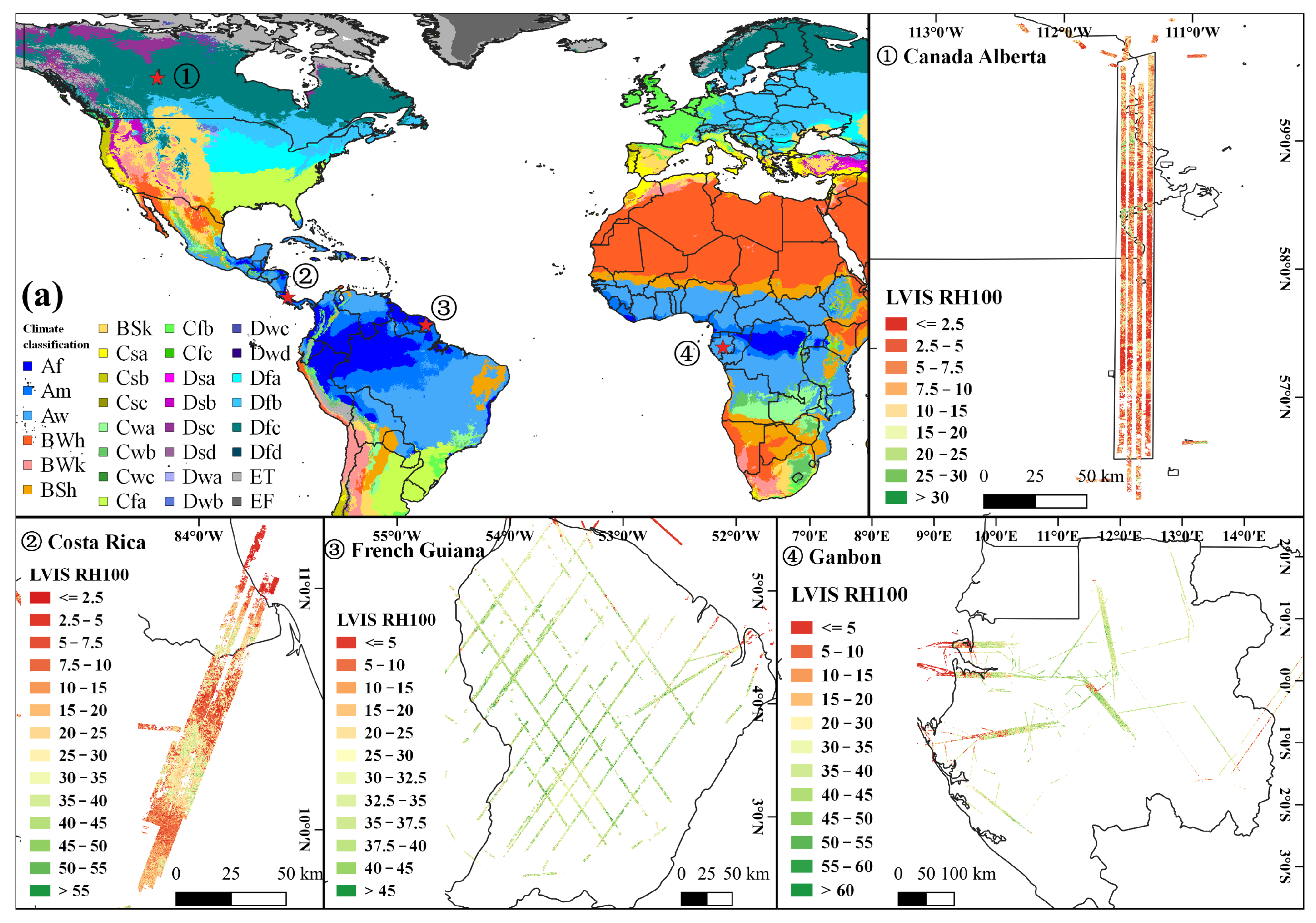
Figure 1 shows our study area. The region ① is located in northeastern Alberta, Canada. This area experiences brief spring and autumn seasons, with a long snow season. The airborne flight area lies between latitudes 56.4° N and 59.7° N, within the boreal coniferous forest zone. The region ② is in Costa Rica, characterized mainly by tropical rainforest and tropical monsoon climates. The coastal areas of Costa Rica are plains, while the central part is separated by rugged mountains. The region ③ is in French Guiana, where 98% of the territory is tropical rainforest with a forest cover rate of 90%. The dry season lasts from August to December, with the remaining months being the rainy season. The average humidity is high, consistently ranging between 80% and 90% throughout the year. The region ④ is in Gabon, characterized by an equatorial humid climate. Approximately 85% of the country is covered by tropical rainforests. The southern part has a tropical savanna climate, while the northern part has a tropical rainforest climate, with annual precipitation exceeding 1500 mm inland and more than 2500 mm along the northern coast.
2.2. Airborne Lidar Data
The Land, Vegetation, and Ice Sensor (LVIS) is an airborne full-waveform imaging LiDAR system developed by NASA to acquire high-precision measurements of land surface topography and vegetation vertical structure. The LVIS data used in the French Guiana, Costa Rica, and Canada study areas (Wood Buffalo region, northeastern Alberta) were acquired aboard the Gulfstream V aircraft platform, with nominal flight altitudes of approximately 10–12 km. In contrast, the LVIS data used for the Gabon study area were collected aboard the NASA Gulfstream III aircraft, with a nominal flight altitude of approximately 8 km.
LVIS operates in two primary instrument configurations: LVIS Facility and LVIS Classic. The LVIS Facility system has a nominal footprint diameter of approximately 10 m, providing higher spatial resolution and enabling detailed characterization of terrain relief and forest canopy structure. In comparison, the LVIS Classic system has a larger nominal footprint diameter of approximately 20 m, which is more suitable for efficient coverage over broad spatial extents. All LVIS datasets were obtained from the official NASA LVIS data portal (
https://lvis.gsfc.nasa.gov/Home/index.html, accessed on 15 April 2024.).
The airborne LiDAR data used in this study encompass both tropical forest regions and boreal forest regions. For the tropical study areas, LVIS Classic data acquired in Costa Rica (June 2019), Gabon (May 2023), and French Guiana (July 2021) were used.
For the Canadian boreal forest study area (Wood Buffalo region, northeastern Alberta), LVIS Facility data acquired during July and August 2019 were employed. These data were collected as part of NASA’s Arctic-Boreal Vulnerability Experiment (ABoVE) 2019 airborne campaign. During this campaign, LVIS conducted an intensive observational deployment over northern Canada and Alaska lasting approximately four weeks, completing a total of 15 flight missions and providing systematic coverage of representative boreal forest and permafrost ecosystems. The acquisition period of the Canada LVIS data closely coincided with the ICESat-2 observation period, thereby effectively reducing temporal mismatch effects associated with forest structural changes.
Both LVIS datasets provide footprint-level measurements of vegetation canopy height percentiles and topographic elevation. In this study, the ZG and RH100 parameters from the LVIS Level 2 elevation and height products were used to represent ground elevation and vegetation canopy height, respectively.
Additionally, the parameters COMPLEXITY, canopy cover, and slope were extracted for subsequent analysis. COMPLEXITY represents the structural complexity of the vegetation canopy. Canopy cover refers to the proportion of ground area covered by the vertical projection of tree crowns.
2.3. ICESat-2 ATL08 Products
The ICESat-2 ATL08 product provides canopy height and terrain measurements along the spaceborne’s orbit, along with other descriptive parameters. Due to noise introduced by factors such as solar radiation affecting the ATLAS, the DRAGANN algorithm is employed to classify ATL03 geolocated photons into ground, canopy, canopy top, and noise categories in order to remove background noise. To ensure sufficient photon points for accurate surface representation, segments with fewer than 50 photons in a 100-m segment are reported as invalid. In this study, for the tropical regions, we selected ICESat-2 ATL08 products (version 6, 2019–2023) within a time window of two years before and after the airborne data acquisition. For the Canada region, ICESat-2 ATL08 products corresponding to the LVIS acquisition period were downloaded. All data used in this study were obtained from NASA’s EARTHDATA (
https://search.earthdata.nasa.gov/) platform. The selected ICESat-2 ATL08 regression parameters are shown in
Table 1. We selected the “h_te_mean” and “h_canopy, 98th percentile relative height” parameters for subsequent research and analysis.
2.4. Data Process
2.4.1. Noise Filtering and Data Selection for ATL08
For the ICESat-2 data, we performed different data filtering procedures for each research area. Initially, we excluded ICESat-2 footprints with high uncertainty by removing data with a canopy height uncertainty parameter (h_canopy_uncertainty = 3.4028235 × 10
38). For the Canadian boreal forests region, we filtered out footprints affected by clouds or aerosols using the cloud flag parameter (cloud_flag_atm < 1). For the tropical regions, we applied a more lenient cloud flag parameter (cloud_flag_atm < 2) to remove footprints affected by clouds or aerosols. Additionally, we excluded data segments affected by atmospheric scattering using the “msw_flag” parameter. Given the substantial uncertainty in terrain and canopy height in the study areas, we removed ATL08 segments with non-
values using the “sub_te_flag” parameter before analyzing elevation data. For canopy height analysis, we further excluded ATL08 segments with non-
values using the “sub_can_flag” parameter. For the Canadian boreal forests and Costa Rica regions, we removed non-vegetated areas such as urban regions and water bodies using the Copernicus Global Land Cover Layers: CGLS-LC100 Collection 3 and the Global 4-class PALSAR-2/PALSAR Forest/Non-Forest Map products. For the tropical region, we utilized the CGLS-LC100 Collection 3, ESA WorldCover 10m v200 (
https://developers.google.com/earth-engine/datasets/catalog/ESA_WorldCover_v200?hl=zh-en, accessed on 1 September 2024) to exclude similar non-vegetated areas. Additionally, for the French Guiana region, where significant discrepancies remained after the above data processing, we excluded ATL08 segments with a “Layer_flag” value of 1. A “Layer_flag” value of 1 indicates the possible presence of clouds or blowing snow.
2.4.2. Data Spatial Matching
Based on the LVIS product, we obtained footprint-level relative height (RH), vertical structural complexity (COMPLEXITY), and ground elevation (ZG), which were rasterized to a 30 m resolution. Additionally, drawing from the work of Montesano et al. [
32], we estimated the footprint-level canopy cover (CC) based on various height thresholds and rasterized these estimates. In this study, we selected canopy cover estimates with height thresholds of ≥1.37m to effectively avoid interference from shrubs, grasslands, and other low-lying vegetation. The rasterization method also follows the approach of Montesano et al. [
32]. (data processing code available at:
https://daac.ornl.gov/cgi-bin/dsviewer.pl?ds_id=1923, accessed on 25 April 2024).
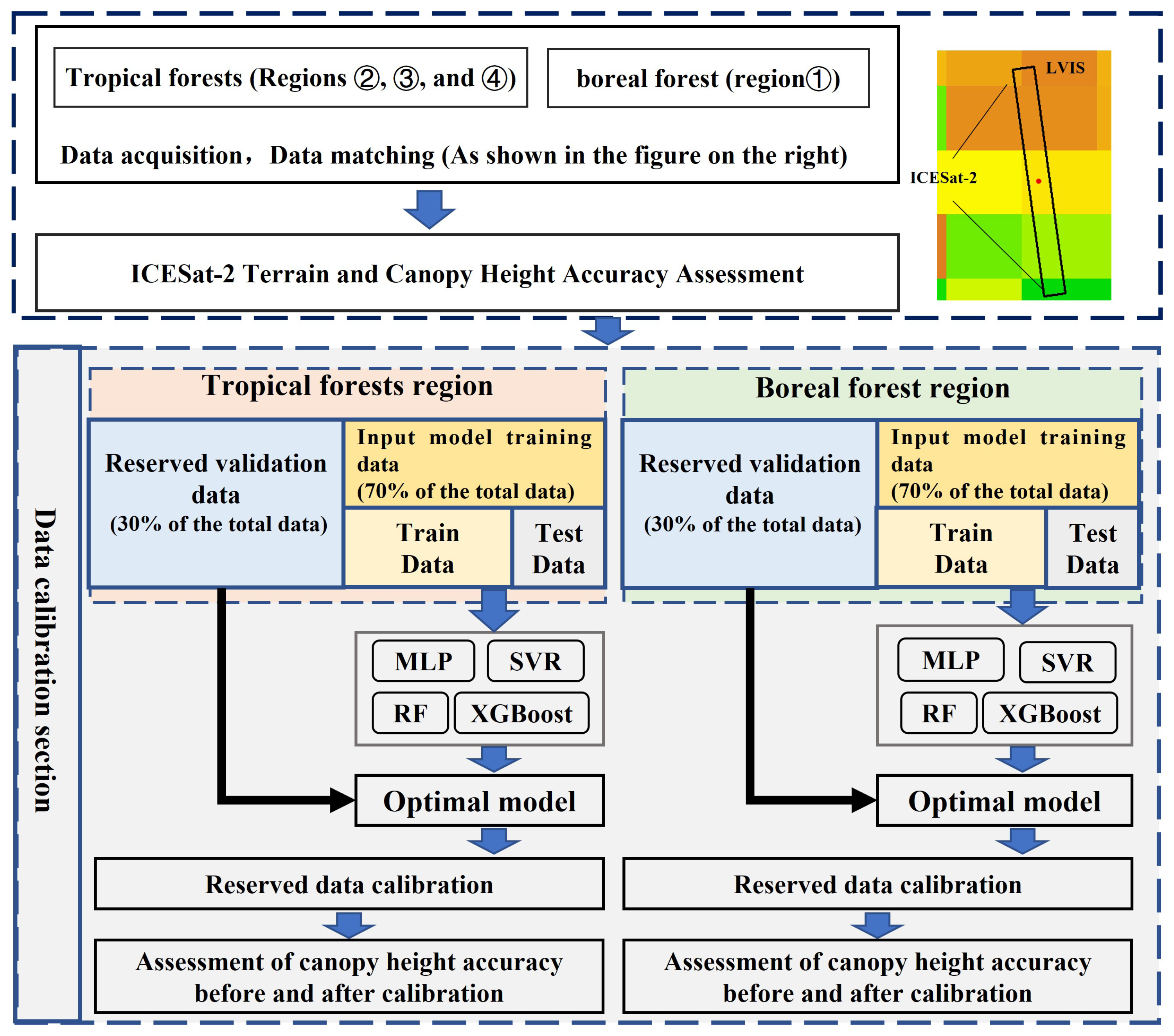
Due to the spatial resolution differences between airborne and spaceborne data, we calculated the mean value of footprint points within a 30 m × 30 m grid for airborne data, while spaceborne data were collected in continuous segments of 100 m × 13 m. The 100 m × 13 m segments were determined by the centroid points of the previous and subsequent ATL08 data segments to obtain the orbital inclination, generating four corner points through the orbital inclination and distance to the centroids, and finally forming the 100 m × 13 m data segment. The airborne raster data were downsampled to a 5 m × 5 m resolution, calculating the mean values of ZG and RH100 within the 100 m × 13 m segment. We also obtained the values of “night_flag”, “sc_orient”, “beamI”, and “segment_snowcover” to distinguish between day/night, strong/weak beams, and snow/no-snow conditions for further analysis.
4. Results
4.1. Terrain Elevation Accuracy Assessment
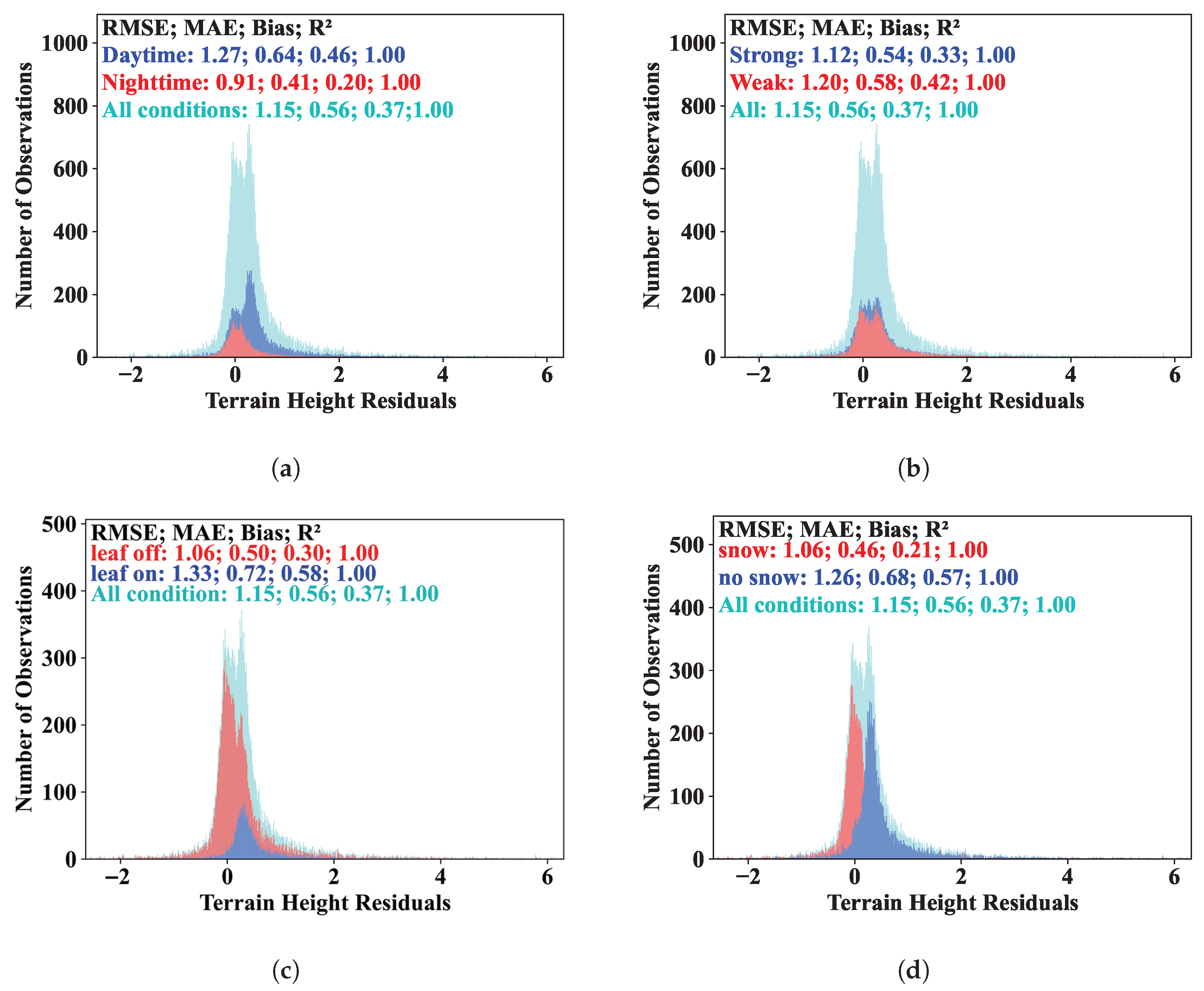
Figure 3 illustrates the errors in the ATL08 terrain estimates for the Canadian boreal forests under various conditions, categorized by: strong/weak beams, daytime/nighttime, snow/no snow, and leaf-on/leaf-off. The leaf-on/leaf-off classification is based on NDVI seasonal variations and precipitation timings, with leaf-on periods from May to September and leaf-off periods from January to April and October to December. A total of 17,185 ATL08 estimates were collected across all beam types and collection conditions. The RMSE and Bias for all data are 1.15 m and 0.37 m, respectively, indicating a high level of agreement between the airborne LVIS data and ATL08 terrain heights. Overall, the terrain data for the Canadian boreal forests shows a notable underestimation, with the underestimation range varying from 0.21 m to 0.58 m. The RMSE across all conditions ranges from 0.91 m to 1.33 m, with only minor variability. For daytime/nighttime conditions, nighttime RMSE (0.91 m) and Bias (0.20 m) are lower than those during the day. For strong/weak beams, the strong beam RMSE (1.12 m) and Bias (0.33 m) are lower than those for weak beams. In the leaf-on and leaf-off conditions, the leaf-off period exhibits lower RMSE (1.06 m) and Bias (0.30 m) compared to the leaf-on period. However, the leaf-on period has the highest RMSE (1.33 m) and Bias (0.58 m) among all conditions. Additionally, comparisons between snow/no snow conditions reveal that RMSE during snow conditions (1.06 m), is slightly lower than during non-snow conditions, with Bias in snowy conditions (0.21 m) being lower than in non-snow conditions (0.36 m). This is due to the increased reflection of photons from snow-covered surfaces, allowing for more accurate representation of the ground. Despite some snow coverage, the estimates are still more accurate compared to non-snow surfaces.
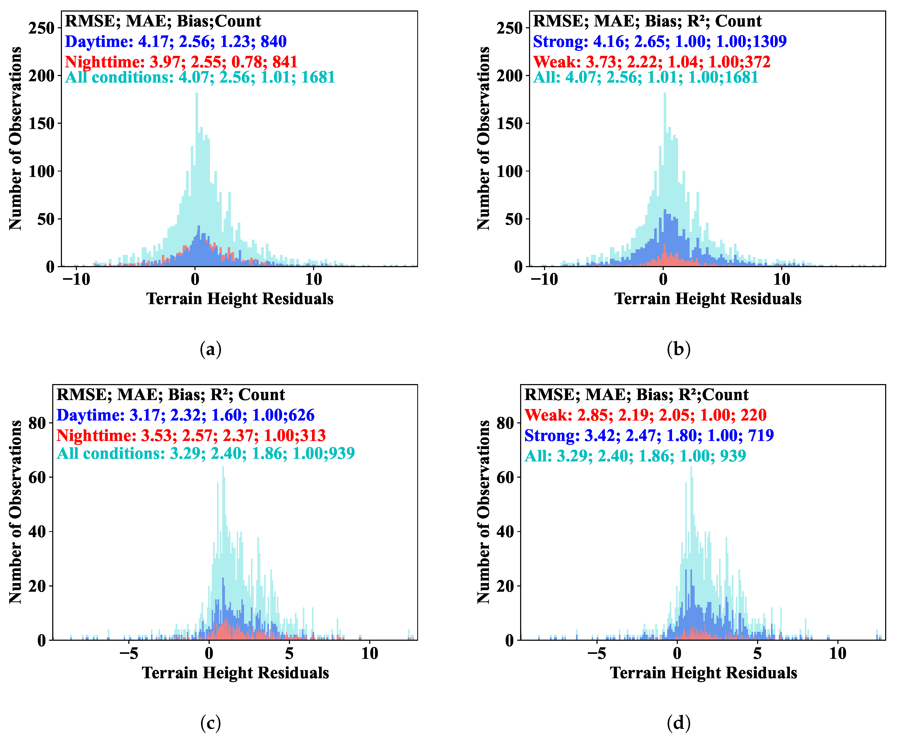
Figure 4 illustrates the estimation errors of ATL08 terrain height in three tropical regions, categorized only by strong/weak beams and daytime/nighttime conditions. Data from Costa Rica are shown in
Figure 4a,b, while data from French Guiana and Gabon are shown in
Figure 4c,d. Hereafter, we refer to the Costa Rica region as Region A and the French Guiana and Gabon regions as Region B. Due to the inherently smaller data volume in tropical regions and the significant reduction in data volume after certain data filtering processes, data from Gabon and French Guiana have been combined, and the number of data points is indicated for each condition. Compared to the ICESat-2 ATL08 terrain accuracy in the Canadian boreal forests region, despite the high consistency between airborne LVIS data and ICESat-2 spaceborne data in tropical regions, the observation accuracy is notably lower. The RMSE estimates for various conditions in region A range from 3.73 m to 4.17 m. For region A: under daytime/nighttime conditions, nighttime RMSE (3.97 m) and Bias (0.78 m) are lower than daytime values, with a data ratio of approximately 1:1 between nighttime and daytime; Under strong/weak beam conditions, weak beam RMSE (3.73 m) and Bias (1.04 m) are lower than strong beam values, with a data ratio of approximately 7:2 between strong and weak beams. For region B, the RMSE estimates for various conditions range from 2.85 m to 3.53 m. For region B: under daytime/nighttime conditions, daytime RMSE (3.17 m) and Bias (1.60 m) are lower than nighttime values, with a data ratio of approximately 1:2 between daytime and nighttime; Under strong/weak beam conditions, weak beam RMSE (2.85 m) is lower than strong beam values, with a data ratio of approximately 3:1 between strong and weak beams. Additionally, there is a noticeable underestimation of terrain data in both Region A and Region B. The underestimation ranges are 0.78 m∼1.23 m and 1.60 m∼2.37 m, respectively, under different conditions.
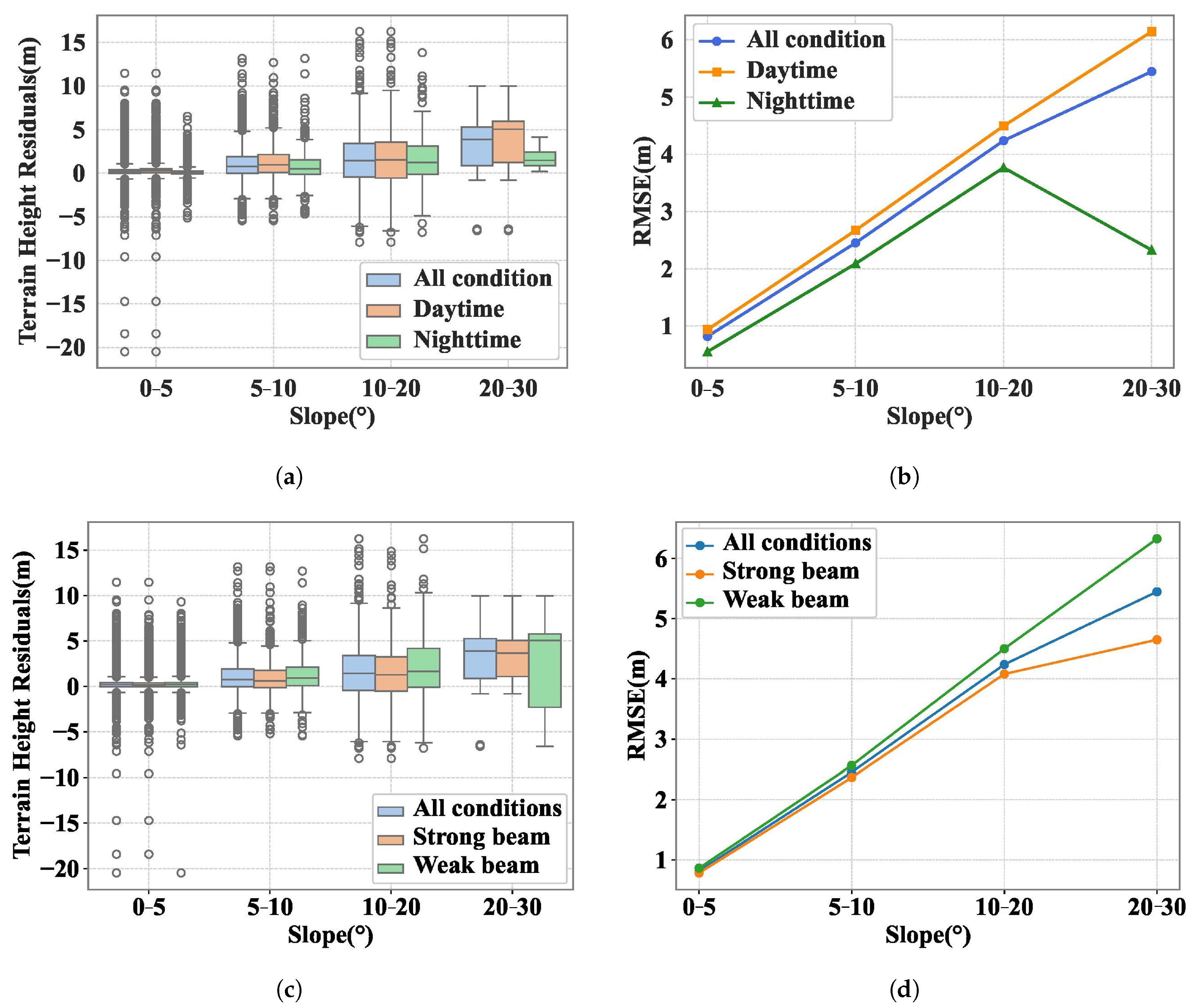
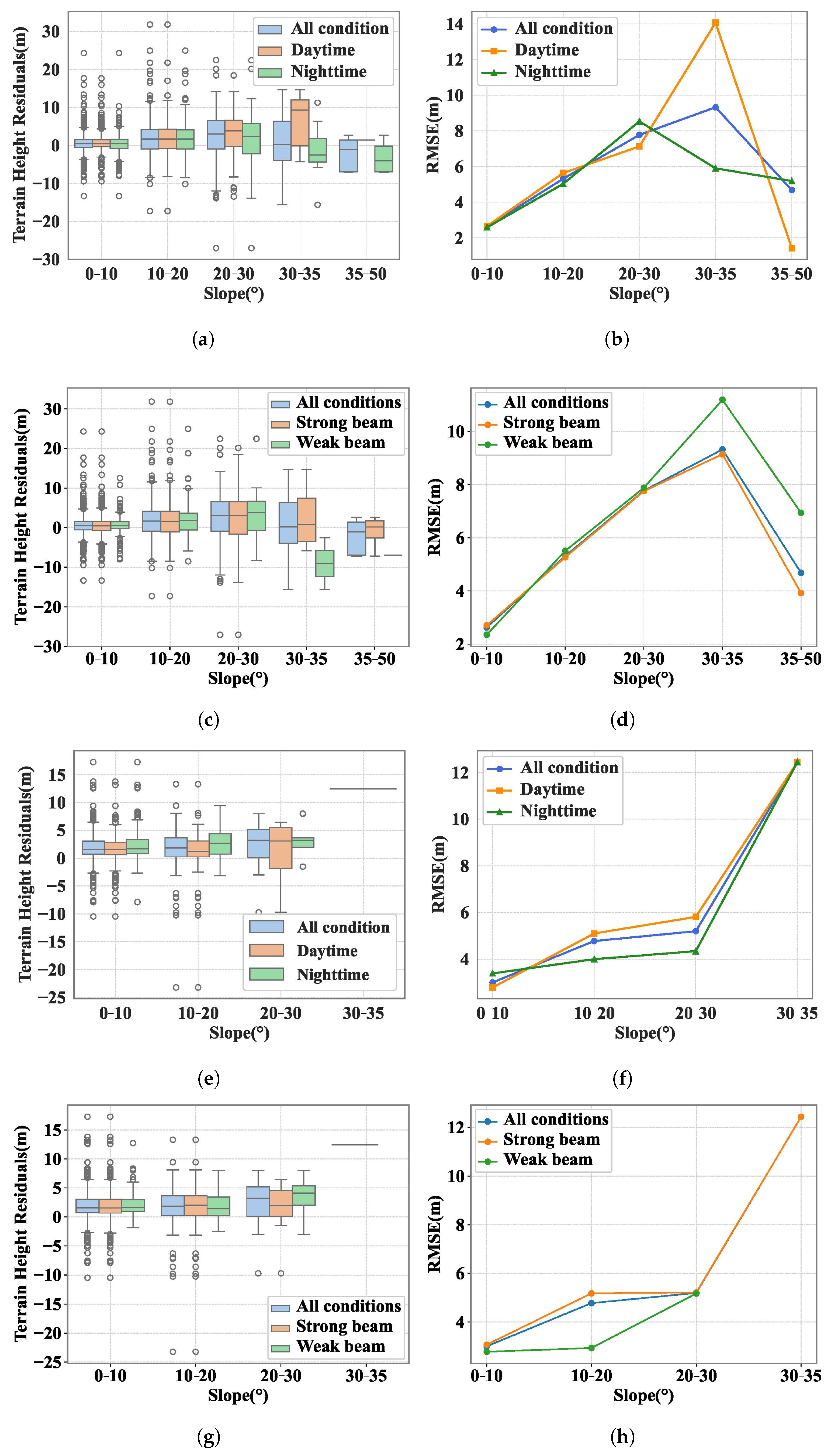
In addition, we observed the ATL08 terrain height estimates across different slope gradients for each region (
Figure 5 and
Figure 6), and recorded the data quantity for each slope class under various conditions (
Table 2 and
Table 3). All conditions clearly indicate that RMSE increases with the increase in slope. Greater terrain variability leads to larger errors in terrain estimation. Even in cases where RMSE decreases with increasing slope, this is primarily due to a decrease in data quantity. In the Canadian boreal forests, the RMSE in the 0–5° slope range is generally below 1 m, while in the Costa Rica region, the RMSE in the 0–5° slope range is around 2 m, and in the Gabon and French Guiana regions, the RMSE in the 0–5° slope range is between 2 and 3 m.
4.2. Canopy Height Accuracy Assessment
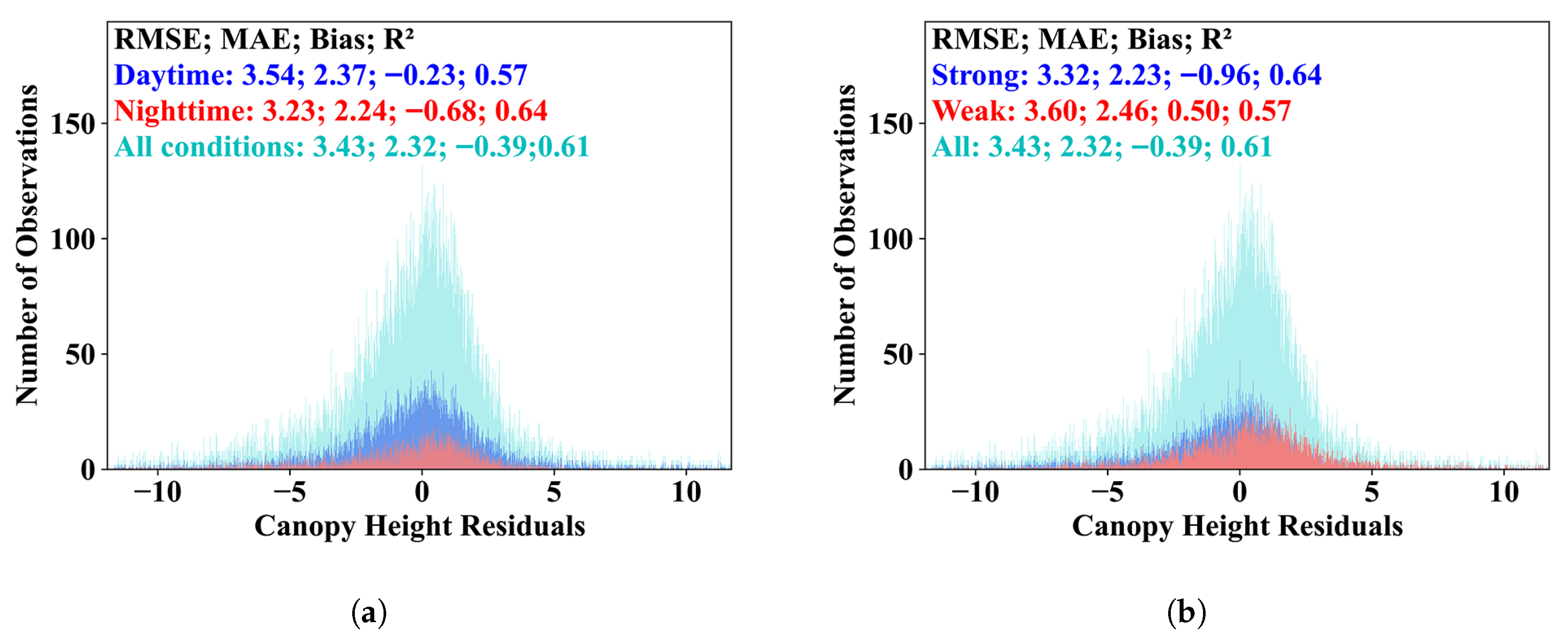
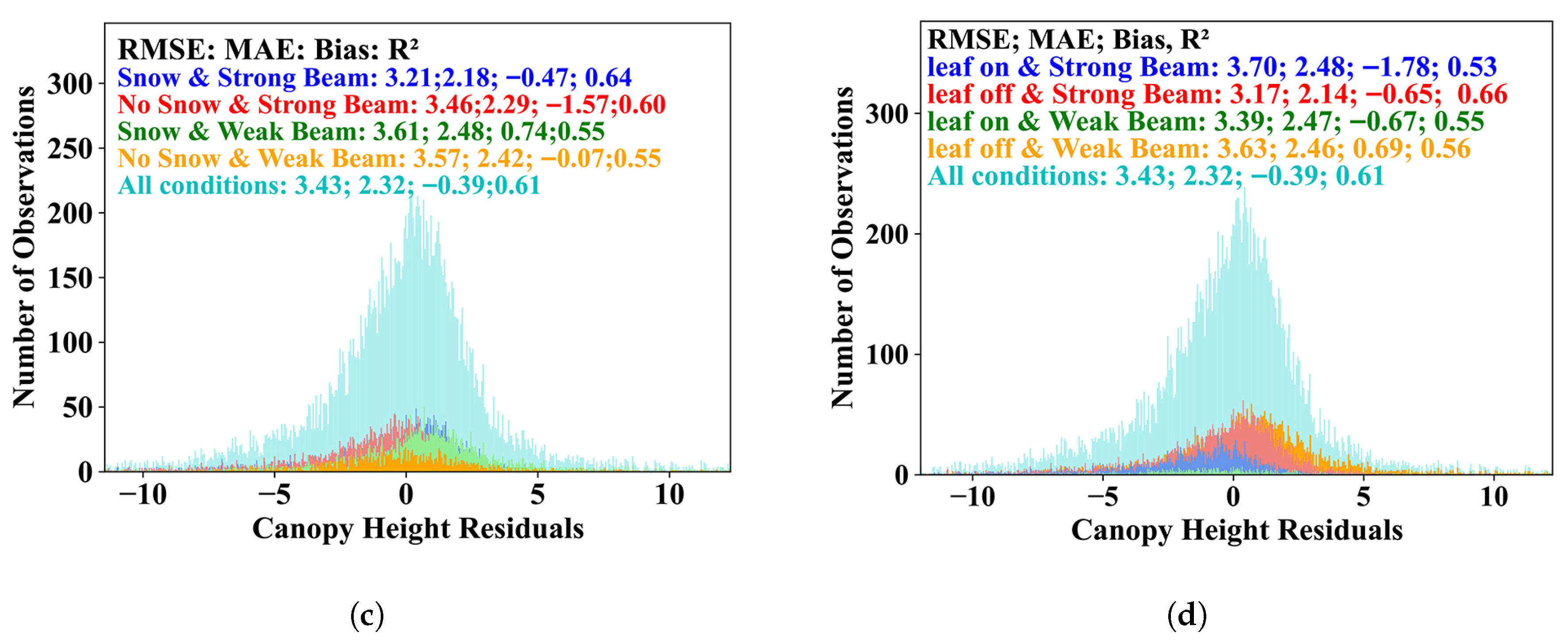
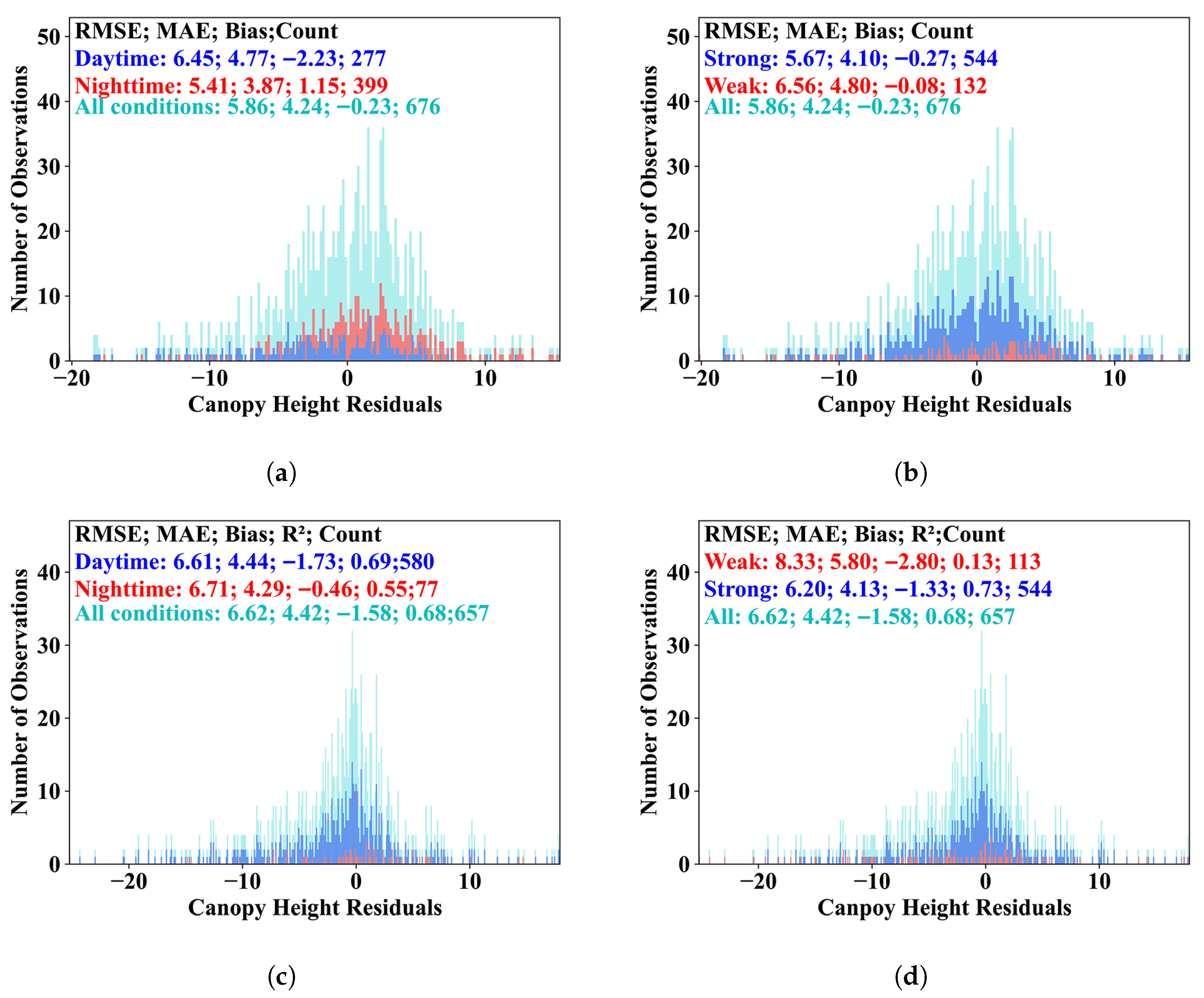
Figure 7 and
Figure 8 illustrate the distribution of canopy height residuals across different regions and observation conditions. In the Canadian boreal forests, the overall RMSE under all conditions is 3.42 m, with nighttime RMSE (3.23 m) lower than daytime RMSE, and strong-beam RMSE (3.32 m) lower than weak-beam RMSE. Under strong-beam conditions, the RMSEs during the snow-covered and leaf-off seasons (3.21 m and 3.17 m, respectively) outperform those under other conditions. The effective photon count of weak beams in snow-covered conditions is approximately 5:2 relative to snow-free conditions, indicating that snow accumulation on the canopy increases surface reflectance and allows ATLAS to receive more photons from the canopy surface.
A similar pattern is observed in Costa Rica, where nighttime RMSE (5.41 m) is lower than daytime RMSE, and strong-beam RMSE (5.67 m) is lower than weak-beam RMSE, with the lowest RMSE occurring under nighttime and strong-beam conditions (5.51 m). The overall RMSE of canopy height residuals in Costa Rica is 2.42 m higher than that in the northern boreal forests. In contrast, in Gabon and French Guiana, daytime RMSE (6.61 m) is slightly lower than nighttime RMSE; however, the number of nighttime ATL08 segments is only 77, meaning that the effective data are far fewer than in daytime. Strong-beam RMSE (6.20 m) remains lower than weak-beam RMSE, with the ratio of strong- to weak-beam segments approximately 5:1.
4.3. Analysis of ATL08 Canopy Height Differences Across Observation Conditions
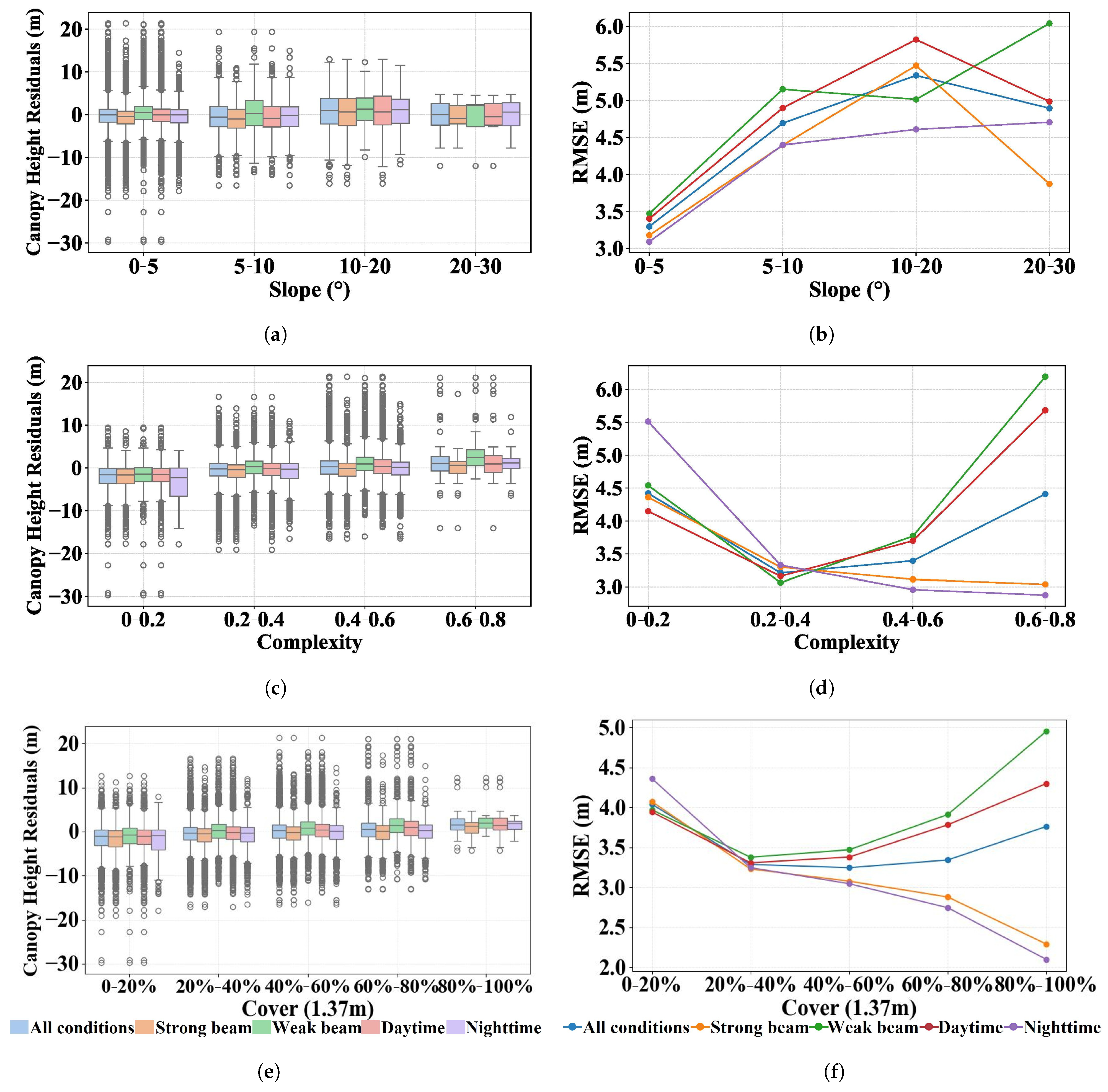
Figure 9 and
Table 4 illustrate the variations in ICESat-2 canopy height estimation errors and photon counts across different slope classes, canopy structural complexities, and canopy cover conditions in the Canadian boreal forests. From the slope-based grouping results, the ATL08 canopy height residuals exhibit a clear positive relationship with terrain slope. As the slope increases, the residuals progressively grow across all observational conditions, with a slight decrease observed at 20–30°, likely due to the limited number of available photons in this interval. Among the four observation modes, weak beams show the most pronounced increase in RMSE at higher slopes, whereas nighttime strong beams remain comparatively stable. Moreover, the number of effective photons decreases substantially with increasing slope, thereby elevating the RMSE. Overall, terrain slope is a key factor influencing the accuracy of ATL08 canopy height retrievals, and the combined effects of terrain occlusion and photon sparsity in steep areas are the primary causes of increased retrieval errors.
Based on the vegetation complexity stratification, all observational conditions exhibit the lowest RMSE values within the complexity range of 0.2–0.6, where the residuals are the most compactly distributed. This indicates that moderate canopy structural complexity is optimal for stabilizing photon signal returns. Notably, under strong-beam and nighttime conditions, RMSE decreases continuously with increasing complexity. This pattern suggests that high signal strength maintains superior penetration ability and measurement stability even in structurally dense canopies. In contrast, weak-beam and daytime observations show a marked increase in RMSE when complexity exceeds 0.6, accompanied by wider residual distributions in the boxplots, indicating that weak signals are more susceptible to occlusion and energy attenuation within dense vegetation. Photon count statistics further reveal that moderate-to-high complexity classes (0.2–0.6) correspond to a substantial increase in effective photon returns, providing richer structural information for canopy height retrieval. Therefore, ATL08 demonstrates stronger adaptability to complex canopy conditions under strong-beam and nighttime observations, whereas weak-beam performance deteriorates most notably in highly complex forest structures.
According to the canopy cover stratification results, RMSE decreases markedly across all observation conditions when cover increases from 0% to 20% to 20%–40%. This indicates that moderate canopy cover enhances the stability of canopy returns and reduces interference from ground echoes, leading to a more compact residual distribution. However, as cover further increases to 40%–80% and beyond, RMSE rises again under weak-beam and daytime conditions, suggesting that high canopy density reduces photon penetration and makes canopy-top detection more difficult, thereby increasing retrieval errors. In contrast, RMSE under strong-beam and nighttime conditions shows a continuous decline across the entire cover gradient, with particularly tight residual distributions at high cover levels. This pattern demonstrates that high-energy beams and low background noise conditions effectively improve penetration and return localization in dense canopies, enabling reliable height retrieval even in forests with >80% cover. Photon count statistics further confirm these observations: weak beams experience the greatest reduction in effective photon returns at high cover, whereas strong beams exhibit comparatively smaller losses, supporting their more stable performance. Overall, moderate cover (20%–40%) provides the most favorable measurement conditions for weak-beam and daytime observations, while strong-beam and nighttime observations maintain high reliability even in densely covered canopies.
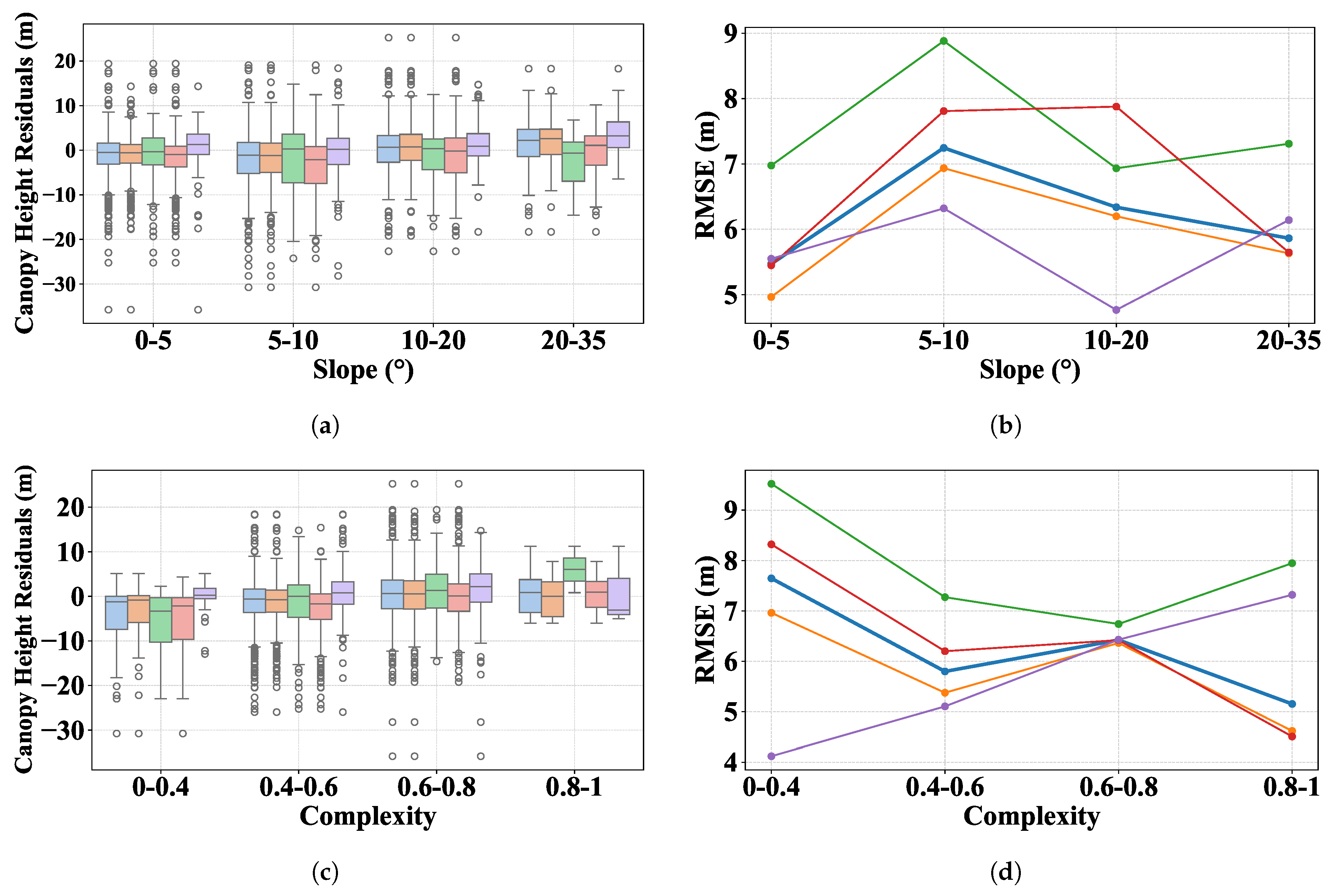
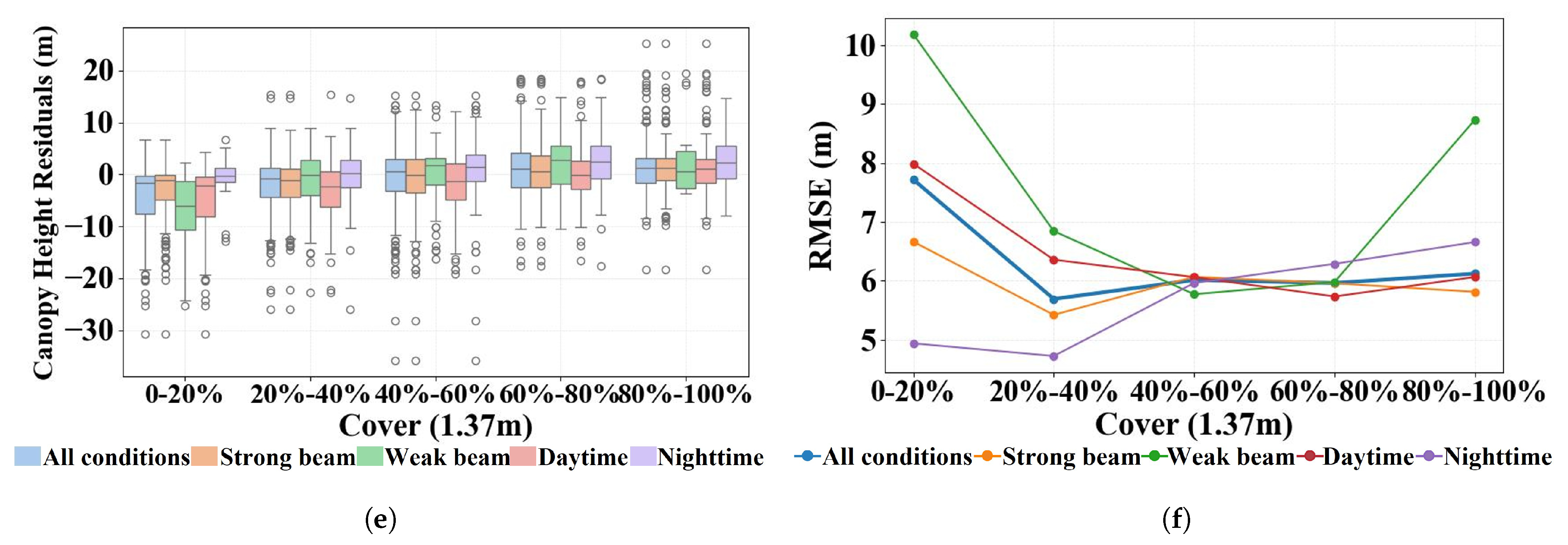
Figure 10 and
Table 5 illustrate the variations in ICESat-2 canopy height estimation errors and photon counts across different slope classes, canopy structural complexities, and canopy cover conditions in the tropical forests. For slope, the residuals are tightly distributed at 0–5°, resulting in the lowest RMSE; however, as slope increases (10–35°), RMSE decreases rather than rises, which may be attributed to the reduced number of photon returns and the potentially lower local canopy density on steeper terrain. In terms of canopy structural complexity, nighttime RMSE increases with increasing complexity, whereas daytime and strong-beam conditions show a decreasing trend. The weak beam exhibits a two-stage pattern, with RMSE first decreasing and then increasing at higher complexity levels. In terms of canopy cover, RMSE is relatively high at low cover (0%–20%). When cover increases to 20%–40% and further to 80%–100%, the canopy becomes more continuous, leading to substantially reduced and more stable RMSE across all conditions. These findings indicate that, under tropical environmental conditions, the error patterns of ICESat-2 canopy height retrievals remain highly uncertain.
4.4. Model Training and Calibration Results
Based on the above analyses, we performed canopy height corrections separately for the tropical regions and the northern boreal forests. Due to the limited number of valid photon points in the tropical region, we combined data from the three regions for training. Using airborne LVIS as the dependent variable and forest canopy structure parameters and terrain parameters extracted from ICESat-2 ATL08 as independent variables (
Table 1), MLP, RF, XGBoost, and SVR models were constructed. The data were randomly split in a 7:3 ratio, with 70% used for model training. In the training process, we further split the data into training and testing sets with a 7:3 ratio and performed 5-fold cross-validation to evaluate the model’s performance.
The comparative results from the model training are shown in
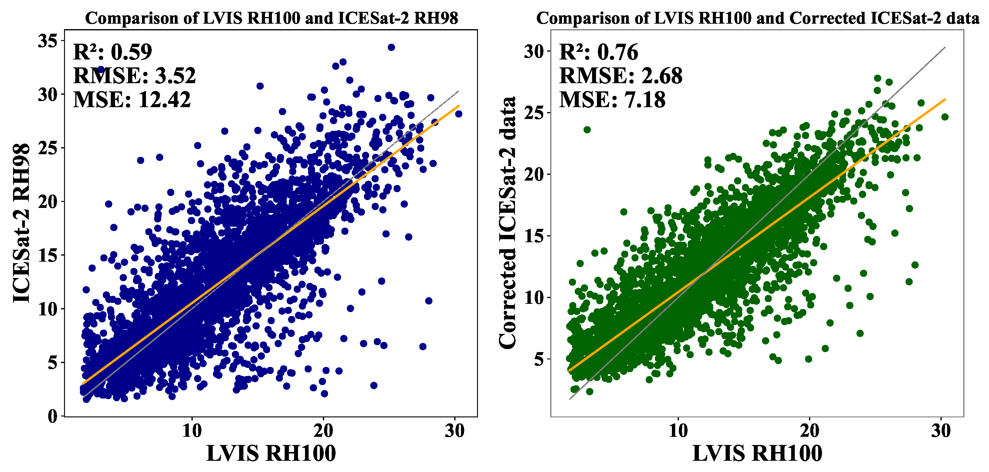
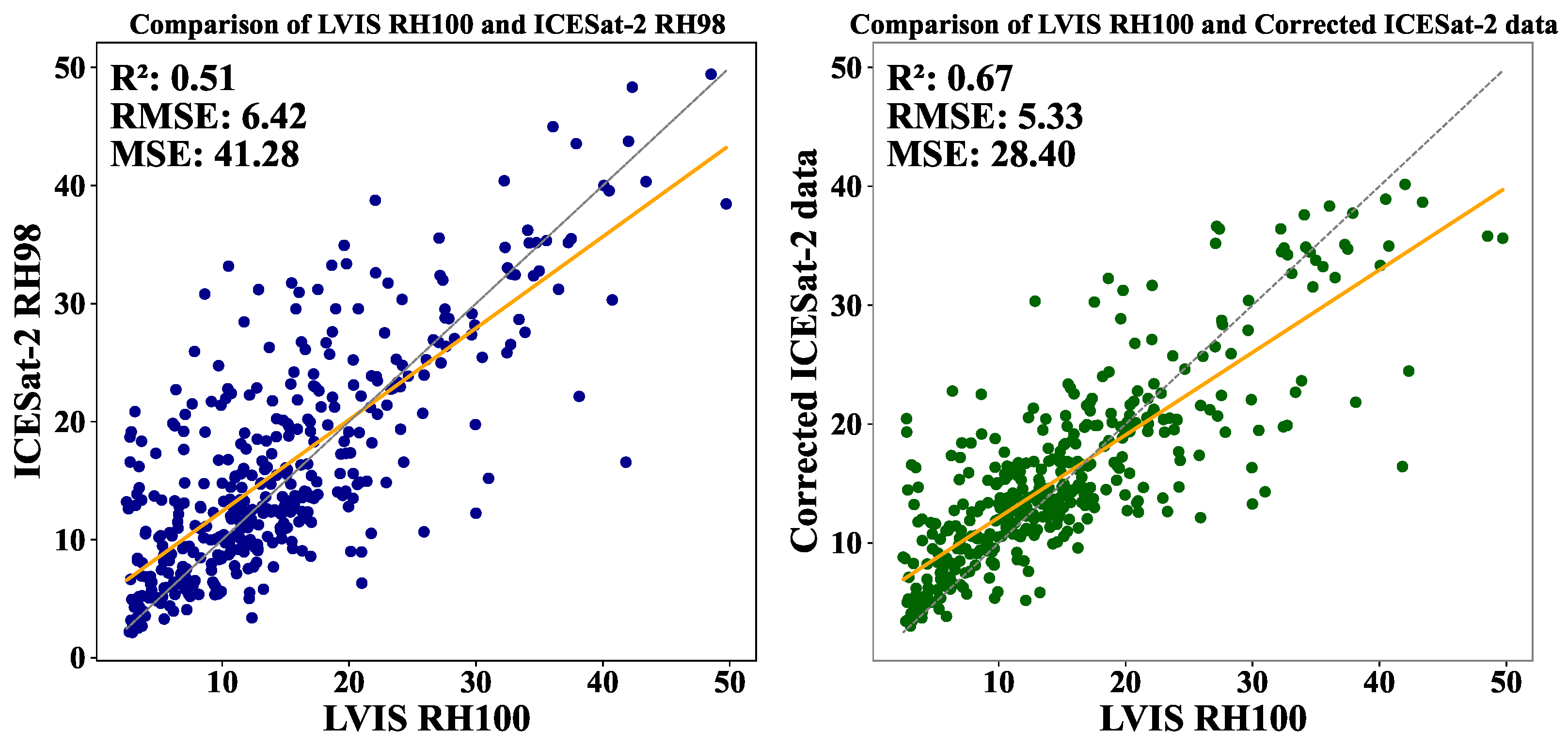
Table 6. The results indicate that the XGBoost model performed better in the Canadian boreal forest region, while the RF model outperformed other models in the tropical region. We selected the best-performing model for each region to calibrate the untrained data, and the results are shown in
Figure 11 and
Figure 12. In the Canadian boreal forest region, the
increased by 17%, and the RMSE decreased by 0.84 m; in tropical regions, the
increased by 16%, and the RMSE decreased by 1.09 m. The calibration results indicate that, compared to the uncalibrated data, the calibrated data exhibits a noticeable improvement in accuracy.
5. Discussion
5.1. Further Filtering Analysis of Tropical Data
We observed that in Gabon and French Guiana, the daytime RMSE was slightly lower than that at night (
Figure 4c and
Figure 8c). Fernández-Díaz et al. [
33] conducted a validation of tropical terrain elevations using extensive high-accuracy airborne data in different tropical regions and reported a similar finding. Unlike our study, Fernández-Díaz et al. [
33] did not remove any abnormal observations in their tropical data analysis. For the tropical dataset, although we applied multiple parameters to filter out data affected by clouds, aerosols, and atmospheric scattering, we set the condition “cloud_flag_atm < 2” to ensure sufficient data volume in tropical regions. As a result, some cloud-contaminated observations remained in the dataset.
Interestingly, after removing all cloud-affected data, we found that over 94% of the daytime data were free from cloud contamination, whereas all nighttime data were affected by clouds. It is unclear whether this represents a unique condition in the specific study year or a more general phenomenon in tropical regions. Moreover, as noted in Fernández-Díaz et al. [
33], high humidity and vegetation physiological activity in tropical forests can cause laser attenuation, and these influences are beyond the scope of the present study. Factors such as cloud thickness and nighttime canopy metabolic attenuation cannot be quantified with our dataset. We believe these factors may partly explain the observed results. Therefore, to improve estimation accuracy in tropical regions, we recommend placing less emphasis on beam strength (strong/weak) and acquisition time (day/night), and instead focusing more on cloud removal and photon availability.
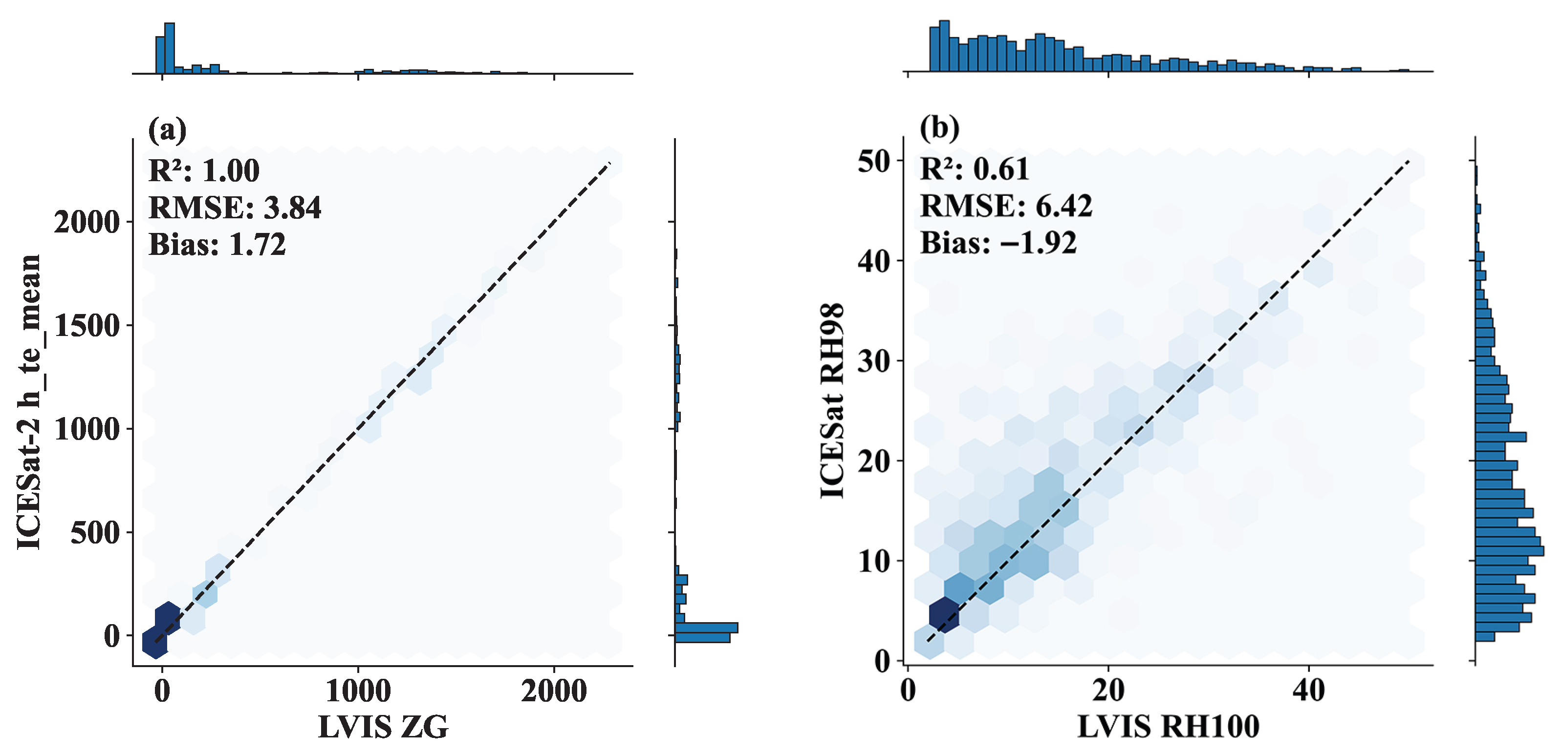
We further evaluated the accuracy of terrain and canopy heights after removing all cloud-contaminated data in tropical regions (
Figure 13), as well as the calibration results (
Table 7). After data processing, the tropical dataset was reduced to only 827 points. The resulting terrain and canopy height
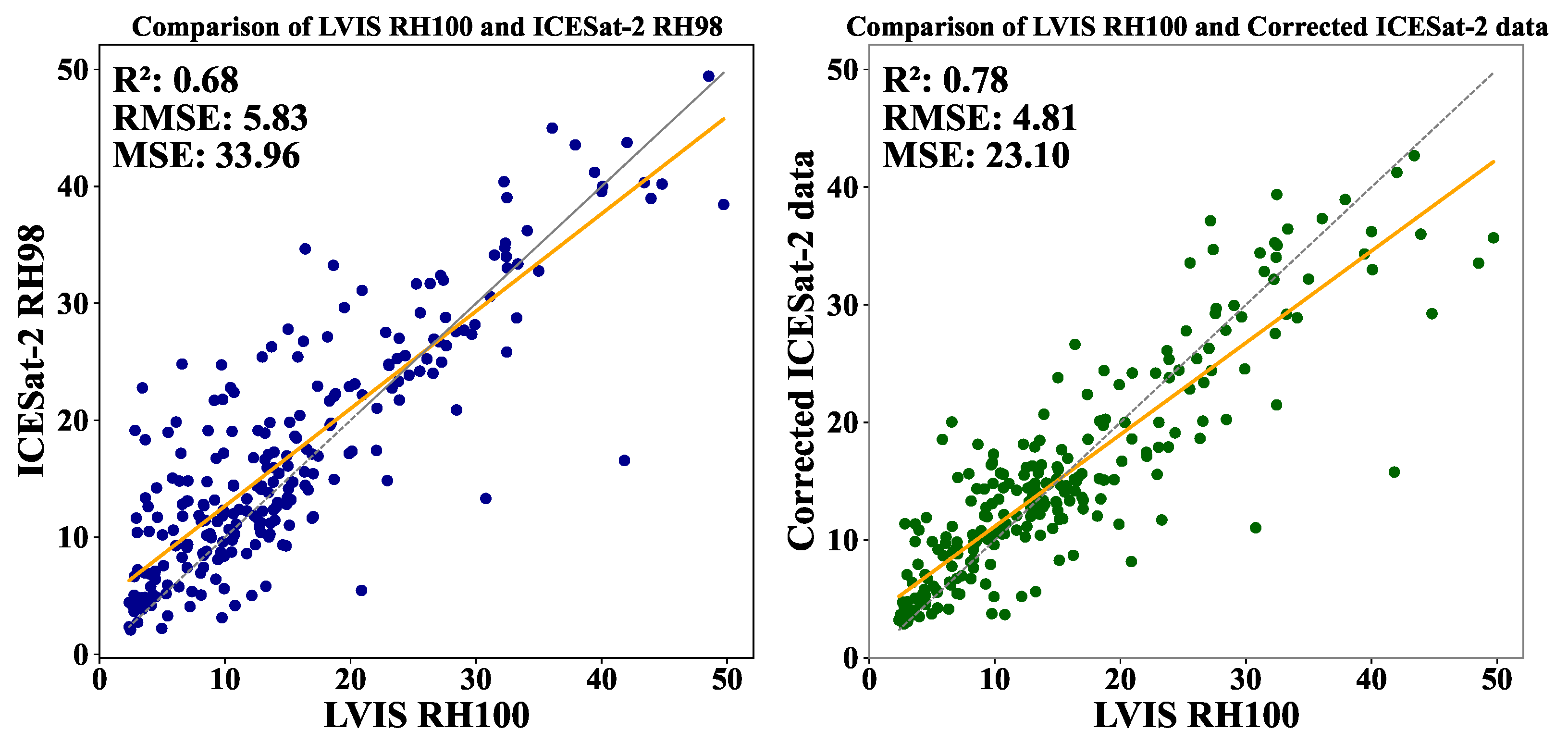
values were 1.00 and 0.61, respectively, indicating strong consistency. When the calibration model was applied to the withheld data for validation, the height error was reduced by 1.02 m (
Figure 14).
By improving the reliability of satellite-based canopy height estimates across contrasting forest biomes, this study provides methodological support for large-scale forest carbon monitoring and sustainable forest management, thereby contributing to climate action (SDG 13) and the conservation of terrestrial ecosystems (SDG 15).
5.2. Limitations
Although this study systematically evaluated the performance of ICESat-2 in retrieving terrain and canopy height across different forest ecosystems and significantly improved its estimation accuracy through machine-learning-based calibration, several limitations remain and warrant further investigation in future work.
First, regarding accuracy assessment, this study relied primarily on a single airborne LiDAR dataset (LVIS) as the reference data. While LVIS provides high spatial accuracy and robust characterization of vertical forest structure, incorporating multiple airborne LiDAR datasets or high-precision field plot measurements would enable cross-validation and further enhance the robustness and reliability of the validation results.
Second, in terms of model generalization and transferability, the LVIS-ICESat-2 calibration models developed in this study still depend on training data from the same or neighboring regions. When applied to areas with substantially different climatic conditions, vegetation types, or forest structural characteristics, model performance may be limited. Future studies could integrate larger-scale and cross-ecoregional training datasets or adopt transfer learning and domain adaptation approaches to improve model generalization across diverse environments.
Third, with respect to model applicability, pronounced differences in canopy structure, species composition, and terrain conditions between boreal forests and tropical rainforests necessitated the development of separate calibration models for each region. Although this region-specific modeling strategy effectively improves local retrieval accuracy, it also increases the complexity of model implementation. Future research could explore hierarchical modeling frameworks or adaptive modeling approaches based on ecological gradients (e.g., canopy cover, structural complexity, and terrain variability) to enhance model generality while maintaining high accuracy.
In addition, future work may integrate the calibrated ICESat-2 canopy height products with forest biomass, carbon stock, and ecosystem functional parameters, thereby extending their applications in global carbon cycle assessments, forest dynamics monitoring, and ecosystem management.