Abstract
As a vital carbon reservoir in terrestrial ecosystems, forest canopy height plays a pivotal role in determining the precision of biomass estimation and carbon storage calculations. Acquiring an accurate Canopy Height Map (CHM) is crucial for building carbon budget models at regional and global scales. A novel UNet++ deep-learning model was constructed using Sentinel-1 and Sentinel-2 multispectral remote sensing images to estimate forest canopy height data based on full-waveform LiDAR measurements from the Global Ecosystem Dynamics Investigation (GEDI) satellite. A 10 m resolution CHM was generated for Chaling County, China. The model was evaluated using independent validation samples, achieving an R2 of 0.58 and a Root Mean Square Error (RMSE) of 3.38 m. The relationships between multiple Relative Height (RH) metrics and field validation data are examined. It was found that RH98 showed the strongest correlation, with an R2 of 0.56 and RMSE of 5.83 m. Six different preprocessing algorithms for GEDI data were evaluated, and the results demonstrated that RH98 processed using the ‘a1’ algorithm achieved the best agreement with the validation data, yielding an R2 of 0.55 and RMSE of 5.54 m. The impacts of vegetation coverage, assessed through Normalized Difference Vegetation Index (NDVI), and terrain slope on inversion accuracy are explored. The highest accuracy was observed in areas where NDVI ranged from 0.25 to 0.50 (R2 = 0.77, RMSE = 2.27 m) and in regions with slopes between 0° and 10° (R2 = 0.61, RMSE = 2.99 m). These results highlight that the selection of GEDI data preprocessing methods, RH metrics, vegetation density, and terrain characteristics (slope) all have significant impacts on the accuracy of canopy height estimation.
1. Introduction
Forests are a vital component of terrestrial ecosystems, playing a critical role in climate regulation, water conservation, and soil erosion control [1]. In the context of global warming, forest ecosystems are essential for mitigating climate change through the sequestration of greenhouse gases such as carbon dioxide (CO2), thereby contributing to the achievement of carbon neutrality [2]. Reliable assessments of forest resources are fundamental to effective management, requiring accurate measurements of structural attributes to evaluate ecosystem status and dynamics [3]. Conventional field-based survey methods are often time-consuming, spatially limited, and constrained in precision, making it challenging to generate consistent and reliable large-scale data [4]. Such baseline information is indispensable for understanding forest ecosystem functions and services, supporting long-term monitoring and the sustainable utilization of forest carbon stocks—objectives of particular significance in advancing China’s dual carbon goals (carbon peak by 2030 and carbon neutrality by 2060). These efforts not only strengthen national climate action but also foster international collaboration and contribute to the global advancement of climate change mitigation strategies.
Thanks to advances in remote sensing—especially spaceborne lidar missions such as GEDI and ICESat-2—wall-to-wall, high-precision mapping of forest height is now achievable [5]. Potapov et al. developed a global 30 m resolution forest height dataset by integrating GEDI canopy height measurements with Landsat-8 OLI data using bagged regression trees, achieving RMSE values ranging from 6.6 to 9.07 m [6]. Wang et al. fused NASA’s GEDI sensor and the ICESat-2 footprint data with Sentinel-1/2 imagery, UAVSAR observations, and terrain variables, attaining RMSE values between 4.85 m and 5.13 m [7]. Liu et al. calibrated ICESat-2 and GEDI height estimates using airborne LiDAR, then integrated them with Sentinel-1/2 data and Digital Elevation Modelderived variables into an AutoGluon-based ensemble model, achieving a validation accuracy of 3.72 m [8]. Tong et al. combined PolSAR volume scattering parameters with GEDI data through a hybrid RVoG-based machine-learning framework, significantly improving estimation accuracy [9]. Lang et al. employed a Bayesian deep convolutional neural network utilizing GEDI L1B waveform data to generate a global canopy height map with RMSE values of 2.7–4.4 m [10]. A multimodal attention-based deep-learning framework named MARSNet was proposed by Chen et al [11]. By combining GEDI, Sentinel-1/2, and ALOS-2 PALSAR-2 data, it generates a canopy height map for Jilin Province with 10 m resolution, yielding an RMSE of 3.76 m and an R2 of 0.58 [11]. Similarly, Cambrin et al. introduced the Depth Any Canopy (DAC) model, which fine-tunes a monocular depth estimation network to enable efficient canopy height prediction from multi-source remote sensing imagery [12].
On a regional level, Lin and his associates produced a forest height map of Nanning City with 30 m resolution. This map was created by combining GEDI and MISR data, and the work achieved an RMSE of 3.52 m [13]. Zhu et al. further extended this approach to produce a national-scale 30 m forest height map through the fusion of GEDI and ATLAS data, with an RMSE of 3.75 m [14]. Fan et al. developed a PRFXception-based deep-learning model that integrates GEDI, ICESat-2, and Sentinel-2 data, generating the first 10 m resolution forest height map for parts of Asia and attaining a regional RMSE of 5.75 m [15]. Collectively, these studies demonstrate the effectiveness of multi-source data fusion combined with deep-learning techniques in enabling high-precision forest height estimation.
Chaling County, situated in Zhuzhou City, Hunan Province, is characterized by hilly terrain, rich forest resources, and diverse vegetation types. Traditional ground-based surveys are often costly and inefficient, posing significant limitations for large-scale canopy height estimation. To address these challenges, this study proposes a canopy height inversion method based on multi-source data fusion and deep learning. By integrating Sentinel-1 SAR data, Sentinel-2 multispectral imagery, and GEDI measurements, a UNet++-based model was developed to generate a high-resolution (10 m) canopy height map for Chaling County. We adopted GEDI’s RH98 value—the elevation where 98% of the returned waveform energy is reached—as a proxy for canopy top height.
The main work and contributions of this paper are as follows: (1). Compared with all existing regional-to-global scale canopy height mapping studies, a novel canopy height estimation approach was developed using the UNet++ deep neural network architecture, which integrates GEDI, Sentinel-2, and Sentinel-1 datasets. (2). A Forest canopy elevation map with a spatial resolution of 10 m was generated for Chaling County. The accuracy of this model surpasses that of the previously employed random forest model. (3). The study further investigated the impact of terrain slope, vegetation coverage, RH ratio, and algorithmic parameters on model performance, revealing correlations between these factors and model accuracy.
2. Materials and Methods
2.1. Study Area and Data
2.1.1. Study Area
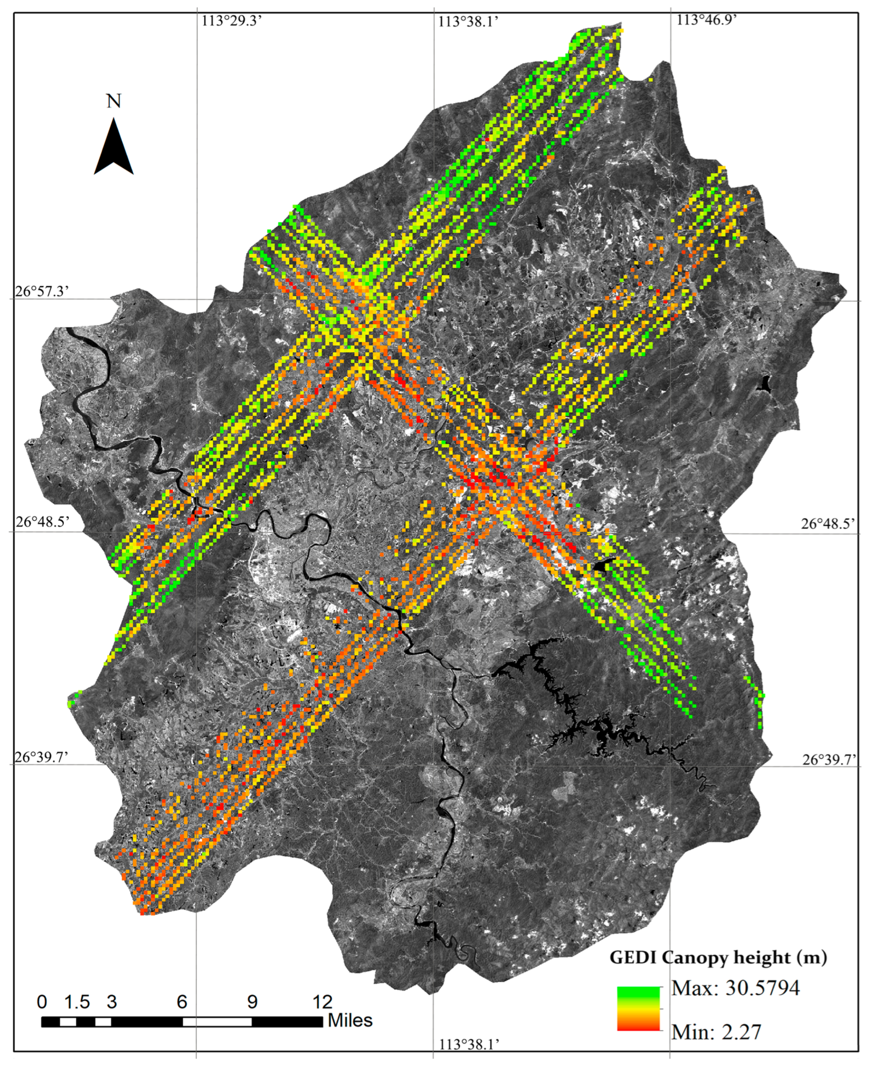
Chaling County, located in the southeastern region of Hunan Province, China, spans geographical coordinates from 113°20′54″ to 113°55′17″ east longitude and from 26°30′26″ to 27°07′25″ north latitude. The county falls within the subtropical monsoon humid climate zone, characterized by short winters, prolonged summers, a frost-free duration of 286 days, an average annual rainfall of ~1370 mm, and an annual sunshine duration of around 1718 h. The topography is predominantly hilly and low mountainous, with rich forest resources. As of 2022, the forest coverage rate of the county reached approximately 62.9%, and the total forest stock volume amounted to 2.23 million cubic meters. Based on topographic classification, the area is primarily categorized as hilly terrain, with the maximum slope ranging between 16° and 30°. The forest distribution in Chaling County exhibits distinct vertical zonation and is predominantly composed of subtropical tree species. The images of Chaling County and GEDI footprints are shown in Figure 1.

Figure 1.
The Sentinel-2 image and canopy heights from GEDI footprints: distribution in Chaling County, China.
2.1.2. Sentinel-1 Data
Sentinel-1 (S1) is a dual-satellite mission launched by the European Space Agency (ESA), comprising Sentinel-1A (launched in 2014) and Sentinel-1B (launched in 2016). Both satellites are equipped with C-band synthetic aperture radar (SAR) and operate in a Sun-synchronous trajectory, providing the constellation revisit interval of approximately 6 days (or 12 days for a single satellite), independent of weather and illumination conditions. In this study, a ground-range detected (GRD) scene with dual-polarization (VV and VH) was employed, offering a spatial resolution of 10 m. Sentinel-1 data were preprocessed using the Google Earth Engine (GEE) platform, following standard procedures including thermal noise removal, radiometric calibration, and terrain orthorectification. Due to the absence of a descending orbit acquisition plan by ESA over the study area in 2020, only two polarization channels were available: VV_ascending and VH_ascending. The image acquisition period spanned from 1 May to 1 October 2020, ensuring coverage of the study area during this timeframe. This period was selected to maintain relatively stable canopy conditions during the leaf-on season while ensuring sufficient image availability. On the GEE platform, a per-pixel multi-temporal median was calculated across images acquired at different times to enhance the smoothing effect of the composite. Subsequently, the processed images were stacked into a two-channel dataset. This approach effectively suppresses outliers and mitigates backscatter variations caused by changes in soil moisture or vegetation dynamics, while also reducing speckle noise inherent in SAR imagery. The backscatter values were clipped to the range of −30 dB to 0 dB and normalized to the [0, 1] interval to ensure consistency with the subsequent Sentinel-2 data [16].
2.1.3. Sentinel-2 Data
The Sentinel-2 (S2) mission constitutes a core component of the Copernicus mission operated by the European Space Agency. It comprises two satellites operating in a Sun-synchronous orbit: Sentinel-2A and Sentinel-2B.S2 delivers multispectral surface reflectance imagery with a swath width of 290 km, providing a combined revisit interval of approximately five days, thereby facilitating frequent monitoring of Earth surface dynamics. The Sentinel-2 data utilized in this study corresponds to Level-2A (L2A) processing, where the reflectance values represent bottom-of-atmosphere estimates derived from ESA’s Sen2Cor processor using Level-1C (top-of-atmosphere reflectance) products [17]. This set consists of 13 spectral bands spanning the visible, near-infrared, and shortwave-infrared sections of the electromagnetic spectrum, with spatial resolutions of 10 m and other categories [18].
By utilizing the Google Earth Engine (GEE) platform [19], we selected Sentinel-2 (S2) images that were temporally aligned with Sentinel-1 images acquired between 1 May 2020 and 1 October 2020. These images covered the study area and exhibited a cloud cover of less than 25%. Following cloud masking procedures, we generated a cloud-free composite image by calculating the pixel-wise median across the image time series. This median compositing approach effectively minimizes the impact of outliers caused by residual clouds or shadows on the resulting imagery. Subsequently, we retained 10 spectral bands with spatial resolutions of either 10 or 20 m. The 20 m resolution bands were resampled to a 10 m resolution to ensure spatial consistency. The selected bands included: B2 (blue), B3 (green), B4 (red); B5–B7 (red edge bands); B8 (broadband near-infrared), B8A (narrowband near-infrared); and B11–B12 (shortwave infrared).
This study did not employ manually constructed vegetation indices (e.g., NDVI) or texture features. Instead, it directly extracted multi-scale and non-linear features from the original Sentinel images using a convolutional neural network (CNN), thereby enhancing the model’s expressive capacity and adaptability. To ensure stability during the neural network training phase, it was necessary to standardize the numerical range of the input data. Specifically, the reflectance values of Sentinel-2 images in the GEE platform are represented as digital numbers (DNs) ranging from 0 to 10,000, which correspond to actual reflectance values calculated as DN/10,000. The typical reflectance range for forested areas is approximately 0 to 0.3 (i.e., DNs between 0 and 3000). To improve contrast and mitigate the influence of outliers, this study applied a DN clipping range of 0 to 5000, followed by normalization to the [0, 1] interval [20]. The resulting Sentinel-2 composite images exhibited uniform scaling, high quality, and were free of cloud contamination, making them suitable as input feature data for deep-learning models.
2.1.4. GEDI Canopy Heights
This study does not use airborne LiDAR but instead employs the spaceborne LiDAR data from the GEDI [21]. The GEDI instrument, operated by NASA, was deployed on the International Space Station (ISS) in December 2018. It provides 1B-level full-waveform LiDAR data, as well as 2A- and 2B-level derived geophysical products, such as canopy relative height (RH) metrics and plant area index, which characterize the vertical structure of vegetation within a 25 m circular footprint. The vertical structure from GEDI was used as a reference to create a continuous canopy height map with a resolution of 10 m through interpolation algorithms. GEDI operates across eight laser channels, with a footprint spacing of 60 m along-track and 600 m cross-track. Due to the orbital constraints of the ISS, GEDI data coverage is limited to latitudes between 51.6° S and 51.6° N.
The relative height indicators (RHn, n = 0~100) provided by the GEDI Level-2A product represent the above-ground height at which the cumulative return energy, from the top of the canopy to the end of the signal, reaches n%. These metrics are derived from the raw waveform data using six distinct combinations of thresholding and smoothing algorithms. The RH values generated by different algorithmic configurations may vary depending on forest type [22].
For this study, GEDI Version 002 Level-2A data were acquired, covering the entire study area during the year 2020. Due to potential atmospheric interference, certain waveform data were deemed unsuitable for characterizing vertical forest structure. Consequently, a set of filtering criteria was applied: (1) quality_flag = 1 and degrade_flag = 0, indicating high data quality with no significant signal degradation; (2) absence of a defoliation flag, ensuring that vegetation was in its growing season during data acquisition; (3) elevation difference less than 50 m, to maintain terrain consistency across observations; and (4) sensitivity ≥ 0.95, to ensure selection of strong and responsive signals capable of penetrating the canopy and reflecting meaningful surface and vegetation structure information. These filtering criteria collectively ensured that the GEDI data used for analysis were of high precision and reliability. Furthermore, recent studies have demonstrated that GEDI-derived canopy height estimates are not significantly influenced by minor topographic slopes [23]. A total of 10,694 GEDI measurements are chosen in the research region.
2.1.5. Auxiliary Data
The Shuttle Radar Topography Mission (SRTM) data, derived using single-pass interferometry technology, covers approximately 80% of the global land surface between latitudes 60° N and 56° S, and is widely utilized in the generation of global digital elevation models [24]. In this study, SRTM products were obtained via the GEE platform to extract topographic elevation and slope information for the study area.
Numerous studies have concentrated on developing 30 m resolution canopy height products for the China region by exploring multi-source remote sensing data fusion techniques and modeling strategies aimed at improving inversion accuracy. For example, Zhu applied a random forest model that integrated spaceborne LiDAR data from GEDI and ICESat-2, with optical imagery from Landsat-8 and the Sentinel satellites, to produce a national forest canopy height map, achieving a validation accuracy of R2 = 0.38 and RMSE = 2.67 m [14]. Liu et al. introduced a deep-learning-based interpolation inversion approach that combined GEDI and ICESat-2 LiDAR footprint data to generate another 30 m resolution forest canopy height dataset for China, with an accuracy of R2 0.60 and RMSE 4.88 m [25]. Furthermore, Potapov et al. developed a global forest canopy height product (Global Forest Canopy Height, GFCH) by integrating GEDI and Landsat data for global canopy height estimation [6]. In our study, to evaluate and confirm the precision of the canopy height maps generated by the proposed model, we used the administrative boundary vector mask of Hunan Province, China, to extract forest height data from the three aforementioned publicly available datasets within the study area. All datasets were resampled to a 10 m spatial resolution using bilinear interpolation and served as reference data for accuracy assessment.
2.2. Method
2.2.1. Technical Workflow
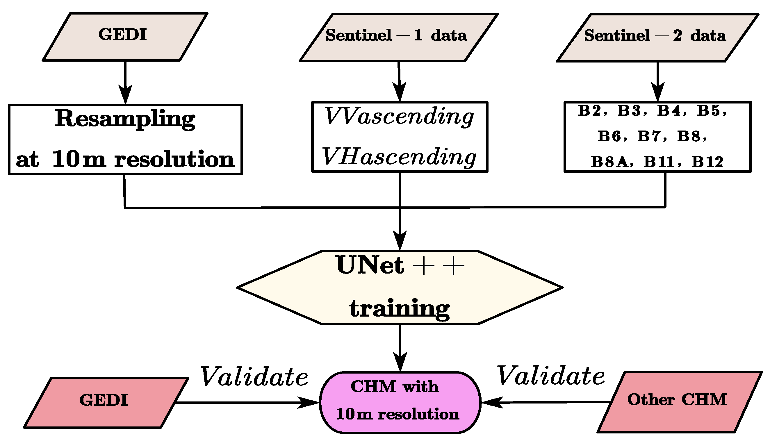
The technical workflow of this study is illustrated in Figure 2.

Figure 2.
The technical workflow.
2.2.2. The Algorithm
First, the GEDI canopy height needs to be interpolated and resampled to a 10 m resolution to ensure the same spatial resolution as S1 and S2. Secondly, the C-band radar signal of S1 data can penetrate part of the tree canopy and is sensitive to both the canopy structure and surface roughness. Among the two channels extracted from S1 data, VV polarization mainly reflects the surface scattering of the bare soil and flat ground, as well as the vertical structure of the trunks and branches; VH polarization is more sensitive to volume scattering and can reflect the complexity of the canopy leaves and foliage layers. Therefore, S1 can provide structural and moisture information of trees, which is helpful for distinguishing tree canopy areas from low vegetation or bare land. Among the 10 channels extracted from S2 data, the visible light bands B2–B4 are related to the pigment content of leaves (chlorophyll, etc.) and can distinguish vegetation types and health conditions. The red-edge bands B5–B7 are highly sensitive to the photosynthetic capacity of leaves, canopy density, and leaf area index. The near-infrared bands B8–B8A are affected by canopy structure and leaf arrangement and can indirectly reflect the volume of the tree canopy. The shortwave infrared bands B11–B12 are related to moisture content and biomass and help identify different forest types and vegetation densities. These spectral features are closely related to vegetation coverage, leaf area index, and biomass, and these indicators can reflect the height of the forest canopy. Canopy height has a strong correlation with biomass, vegetation coverage, and structural complexity. S1 data is sensitive to structure, and S2 data is sensitive to leaf area and canopy status.
Then, by inputting the above 12 selected channels into the UNet++ network for training, local spatial features such as texture and spectral–structural combined features are automatically extracted. Taking the RH information in the GEDI data as the label data, through deep learning with a large number of samples, the model learns to combine texture, spectrum, and height, and thus can predict canopy heights by only inputting S1 and S2 data.
2.2.3. The UNet++ Network
In this study, the UNet++ model was employed to predict forest canopy height through pixel-wise regression using multi-source remote sensing imagery. UNet++ improves upon the original U-Net architecture by integrating dense skip connections between the encoder and decoder pathways, which enhances multi-scale feature interaction and fusion, thereby strengthening feature representation and improving regression accuracy [26].
During the encoding phase (contracting path), the input image is processed through two consecutive 3 × 3 convolutional layers with ReLU activation functions, followed by 2 × 2 max pooling with a stride of 2 for spatial downsampling. This procedure is repeated across four hierarchical levels, with the number of feature channels doubling at each subsequent level, enabling progressive extraction of high-level semantic features.
In the decoding phase (expansive path), feature maps are upsampled using bilinear interpolation and concatenated with corresponding encoder feature maps at the same spatial resolution. Unlike conventional U-Net, UNet++ incorporates multiple nested dense blocks within the decoder, enabling the integration of features from varying depths and levels of abstraction into the reconstruction process. Each fusion block comprises two 3 × 3 convolutional layers accompanied by ReLU activation functions, creating a more robust and effective structure, forming a more robust and hierarchical feature reconstruction pathway. Finally, a 1 × 1 convolution layer with ReLU activation ensures non-negative output predictions while reducing the number of feature channels from 64 to 1, yielding the final canopy height map. The detailed network architecture is illustrated in Figure 3.
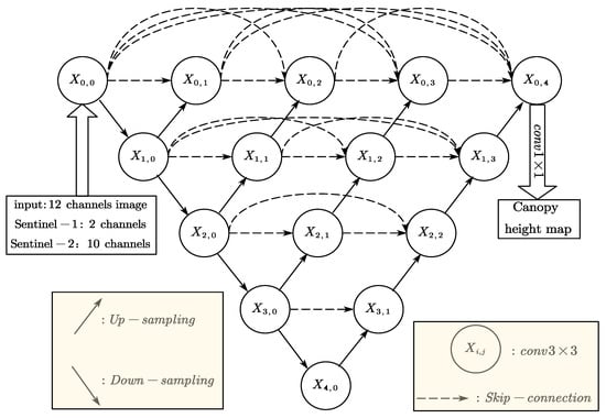
Figure 3.
The Unet++ network structure.
During training, model predictions are compared with valid pixel labels from the GEDI dataset, and the mean absolute error (MAE) is used as the loss function. Optimization is performed only on pixels that have valid reference values.
During training, the model outputs are compared to valid pixel labels from the GEDI dataset. The mean absolute error (MAE) is employed as the loss function, and optimization is performed exclusively over regions with valid observations.
2.3. Training Process
The model training workflow is shown in Figure 4:

Figure 4.
The UNet++ network training process.
According to the workflow presented in Figure 4, the steps for training are as follows: (1) Four representative regions across the entirety of Chaling County were selected based on the availability of Sentinel-1 (S1), Sentinel-2 (S2), and GEDI data. Each selected region covered an area of 2560 × 2560 pixels at a spatial resolution of 10 m. These regions were subsequently divided into 400 smaller patches of 256 × 256 pixels. To improve training reliability and reduce model overfitting, a filtering step was applied to ensure that each patch contained at least one valid GEDI footprint. (2) As validated by Schwartz et al., the use of only 14 spectral bands can already yield satisfactory results [20]. Following this insight, a total of 12 channels, comprising relevant bands from both S1 and S2 imagery, were employed as input to the model in this study. (3) The RH98 values from GEDI were projected onto a 10 m resolution grid spatially aligned with the S1 and S2 composite data. Each RH98 measurement was assigned to the grid cell corresponding to the center of the circular GEDI footprint. (4) The model’s output was compared against the gridded GEDI canopy height reference only at pixel locations where RH98 values were available. The Mean Absolute Error (MAE), as defined in Equation (1), was adopted as the loss function to quantify prediction accuracy.
where represents the total count of GEDI data. The model was trained using the Adam optimizer [27], in combination with a learning rate scheduler. To mitigate the risk of overfitting, an early stopping mechanism was implemented, which terminated the training process if the validation loss failed to improve within a predefined number of epochs. During each training cycle, 400 image patches were used, with 80% randomly allocated to the training set and the remaining 20% allocated to the validation set.
2.4. Evaluation Metrics
To comprehensively assess the forecasting accuracy of the suggested model on the test dataset, a set of widely recognized evaluation metrics was utilized. These metrics include the Mean Absolute Error (MAE), Root Mean Square Error (RMSE), Mean Error (ME, which measures prediction bias), and the coefficient of determination (R2, which assesses the linear relationship between predicted and actual canopy heights). Specifically, MAE represents the mean magnitude of prediction errors without regard to their direction, whereas RMSE emphasizes larger errors by taking the square root of the average squared errors. ME provides insight into the systematic bias of the model, revealing whether it tends to overestimate or underestimate canopy heights. R2 quantifies the correlation between predicted and observed canopy heights, with higher R2 values indicating a stronger correlation and, thus, better model performance. The formula for R2 is shown in Equation (2).
In Equation (2), denotes the observed value, represents the predicted value, is the mean of the observed values, and signifies the sample size. The coefficient of determination R2 ranges from 0 to 1; values closer to 1 indicate that the model explains a larger proportion of the variability in the data.
Root Mean Square Error (RMSE) quantifies the variability between predicted values and observed values, which is defined by Equation (3):
It serves as an indicator of the deviation between predicted and observed values, where lower values reflect improved accuracy in model predictions. The Mean Absolute Error (MAE) represents the average of the absolute differences between predicted and observed values, as defined in Equation (4):
The MAE provides an intuitive measure of the average magnitude of prediction errors, where lower values signify greater predictive accuracy of the model.
3. Results
Following the completion of the full training and validation process to determine the optimal model parameters, the model was applied to Sentinel-1 and Sentinel-2 data covering the entire Chaling County. This application generated a canopy height map at a 10 m spatial resolution for the entire study area. The canopy height map of Chaling County with a spatial resolution of 10 m is illustrated in Figure 5.
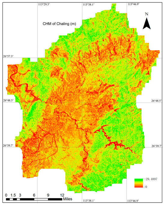
Figure 5.
The Canopy Height Map of Chaling County at a 10 m spatial resolution, generated using the method proposed in this study. Detailed information regarding preprocessing steps and the training process is provided in Section 2.3. A comprehensive overview of the CHM generation workflow is provided in Section 2.2.1.
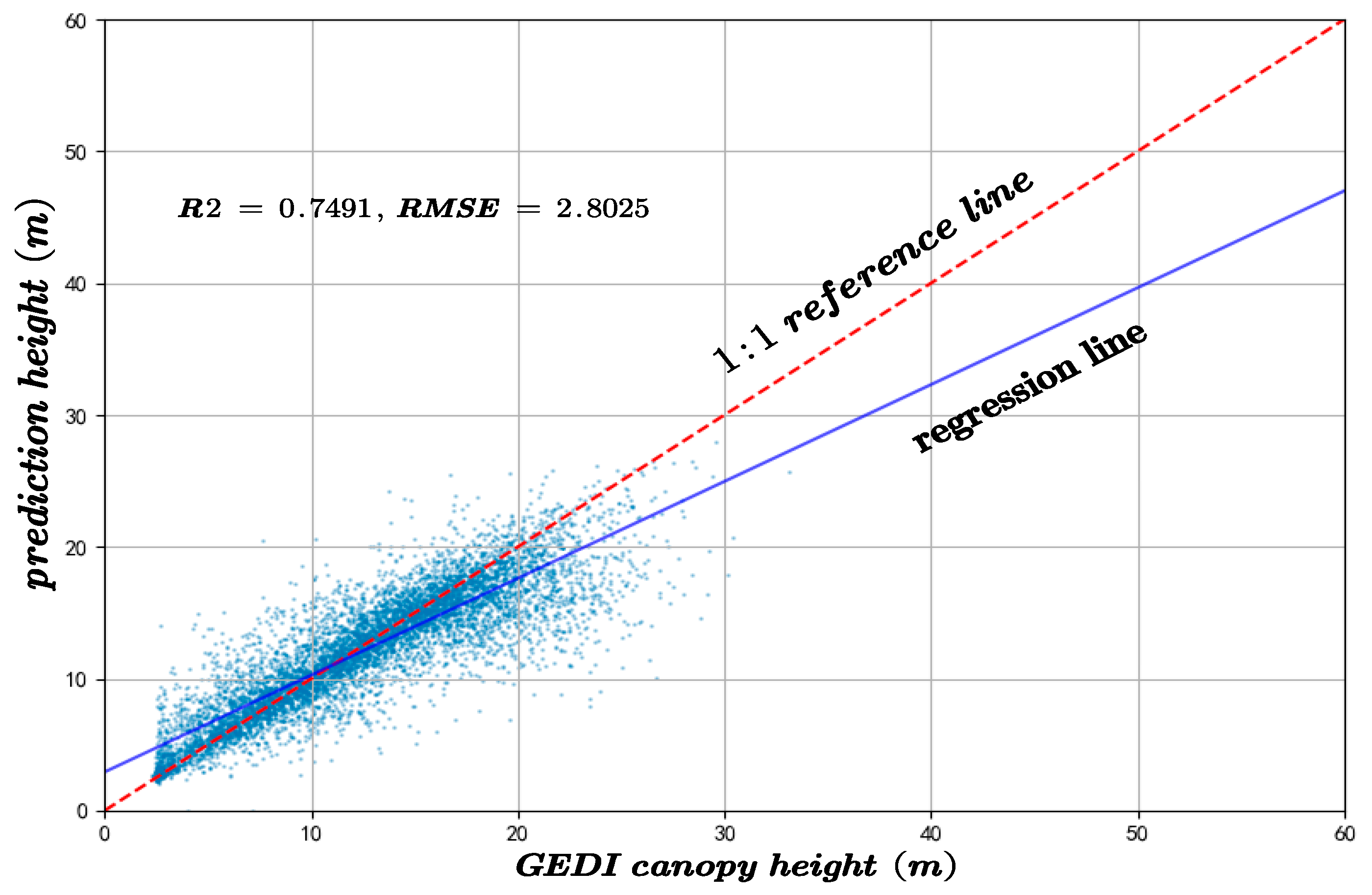
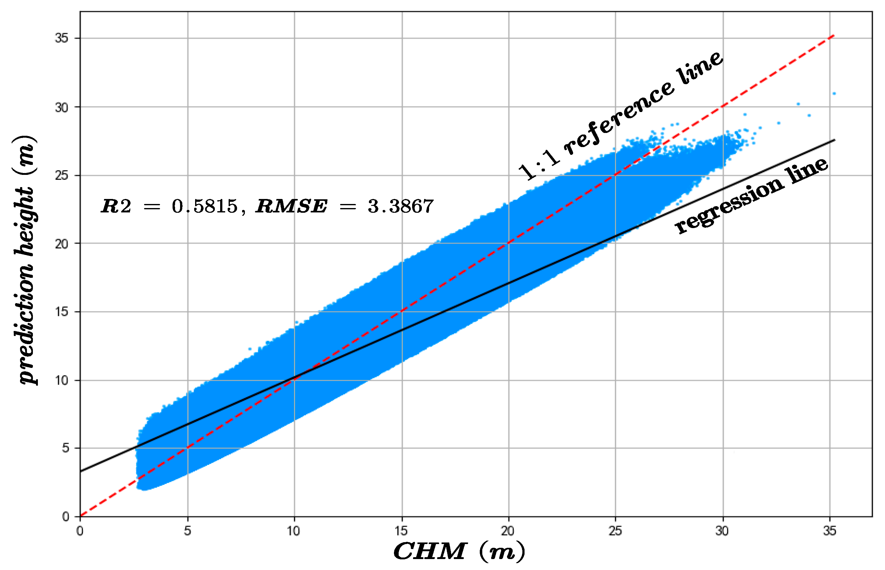
The predicted canopy heights were validated against two independent datasets: GEDI observations and an auxiliary canopy height model (CHM). The results of the accuracy assessment are displayed in Figure 6 and Figure 7.
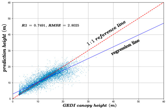
Figure 6.
The inversion accuracy of forest canopy height across the whole experimental area compared to the GEDI canopy height.
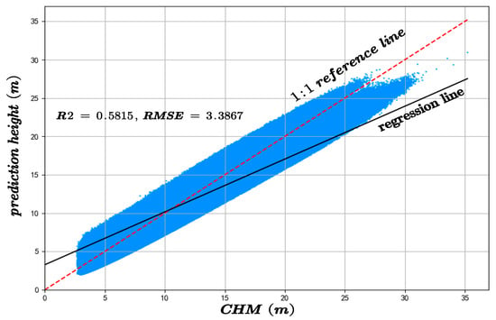
Figure 7.
The inversion accuracy of forest canopy height across the whole experimental area compared with the CHM.
4. Analysis
4.1. Independent Verification Results and Ablation Experiments
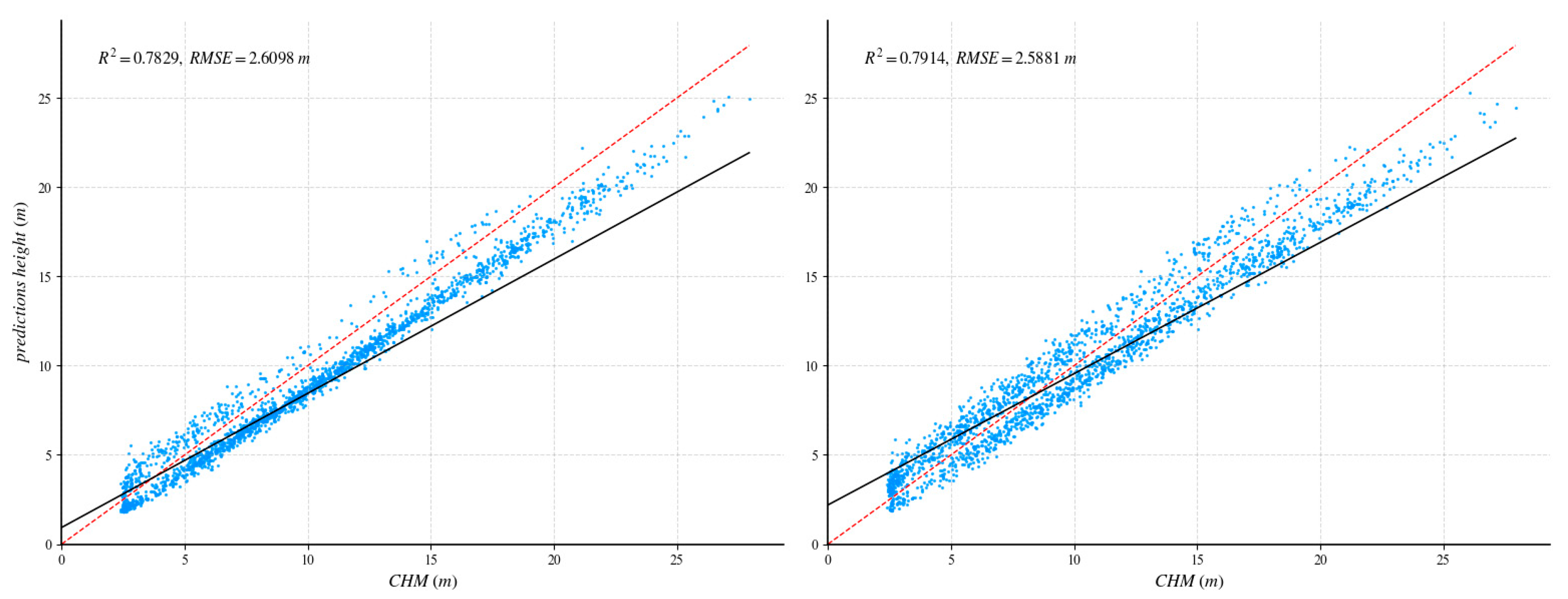
After UNet++ training was complete, the learned weights were tested on a fully independent scene containing 1859 reliable GEDI footprints. To quantify the benefit of our method, we repeated the process with a standard U-Net: identical training/validation tiles, the same independent area, and a shared evaluation protocol. Figure 8 and Figure 9 report the head-to-head comparison, confirming a clear accuracy margin in favor of the proposed method.
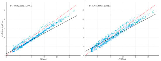
Figure 8.
Comparison of independent regions with GEDI data validation and ablation experiments. The red dotted line is 1:1 reference line. The (left) side shows the UNet++ network, and the (right) side shows the U-net network.
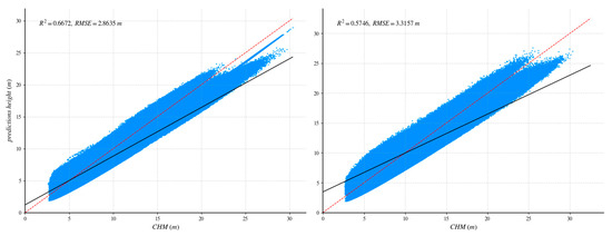
Figure 9.
Comparison of independent regions with CHM data validation and ablation experiments. The red dotted line is 1:1 reference line. The (left) side shows the UNet++ network, and the (right) side shows the U-net network.
4.2. Different Relative Height
In order to evaluate the accuracy of tree height inversion using different relative height metrics, five GEDI L2A RH indicators were selected and validated against reference canopy height model (CHM) data. The results demonstrate that inversion accuracy varies across the metrics: RH98 exhibited the highest performance, achieving a coefficient of determination (R2) of 0.56, a root mean square error (RMSE) of 5.83, and a mean absolute error (MAE) of 4.38; in contrast, RH100 produced the lowest accuracy, with R2 = 0.49, RMSE = 7.03, and MAE = 5.19, as summarized in Table 1.

Table 1.
The accuracy of GEDI canopy heights (with different Relative Heights) relative to CHM heights (m).
4.3. Different Algorithm
In order to evaluate the performance of different algorithm configurations in canopy height inversion, four GEDI processing algorithms were applied to all GEDI data within the study area, and their inversion results were validated against airborne LiDAR measurements. According to the GEDI Level 2 User Guide, a selected algorithm value of 10 indicates that the initial processing employed algorithm group 5 (a5), but during subsequent processing, the lowest returned mode, typically corresponding to ground or canopy bottom, was identified as potentially being noise rather than a valid signal. To ensure data reliability, the system automatically switches to a more robust processing mode, recomputing elevation and height metrics using a higher-mode waveform. The switching mechanism helps mitigate noise-induced errors and thereby enhances overall data quality. This case is called the seventh configuration (a10). Among the tested configurations, algorithm group ‘a1’ achieved the highest accuracy (R2 = 0.55, RMSE = 5.54, MAE = 4.39), whereas group ‘a5’ performed the worst (R2 = 0.39, RMSE = 13.13, MAE = 11.13), as shown in Table 2.

Table 2.
The accuracy of GEDI canopy heights (with different Algorithms) relative to CHM heights.
4.4. Different Vegetation Coverage
To assess variations in canopy structure characteristics under different vegetation cover conditions, this study classified GEDI points into three categories based on the Normalized Difference Vegetation Index (NDVI): sparse vegetation areas with NDVI values ranging from 0.25 to 0.5, moderate-density vegetation areas with NDVI values ranging from 0.5 to 0.75, and high-density vegetation areas with NDVI values ranging from 0.75 to 1. Figure 10 presents the results for these three NDVI intervals, showing the predicted canopy heights along with the corresponding coefficients of determination (R2) and RMSE) calculated against GEDI observations.

Figure 10.
The model prediction accuracy compared with GEDI data under different NDVI values. The red dotted line is 1:1 reference line.
The figures are arranged from left to right according to the NDVI intervals of 0.25–0.5, 0.5–0.75, and 0.75–1. Figure 11 illustrates a comparison of prediction accuracy between the forecasted outcomes and the canopy height model (CHM) under the same NDVI grouping conditions.

Figure 11.
The model prediction accuracy compared with CHM data under different NDVI values. The red dotted line is 1:1 reference line.
Figure 12 shows the number of samples under different NDVI classifications.
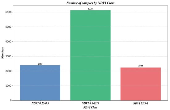
Figure 12.
Number of samples under different NDVI.
4.5. Different Slopes
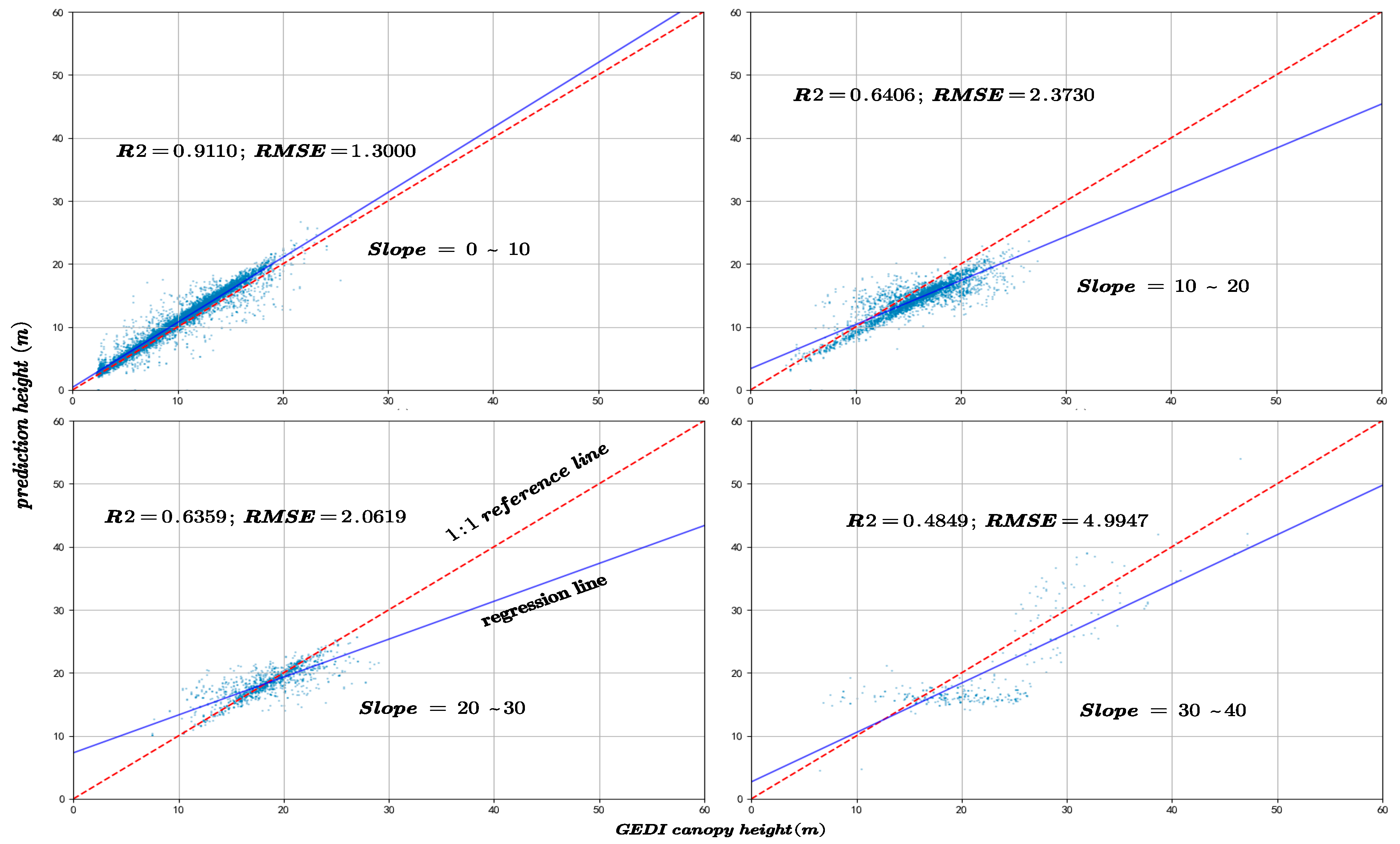
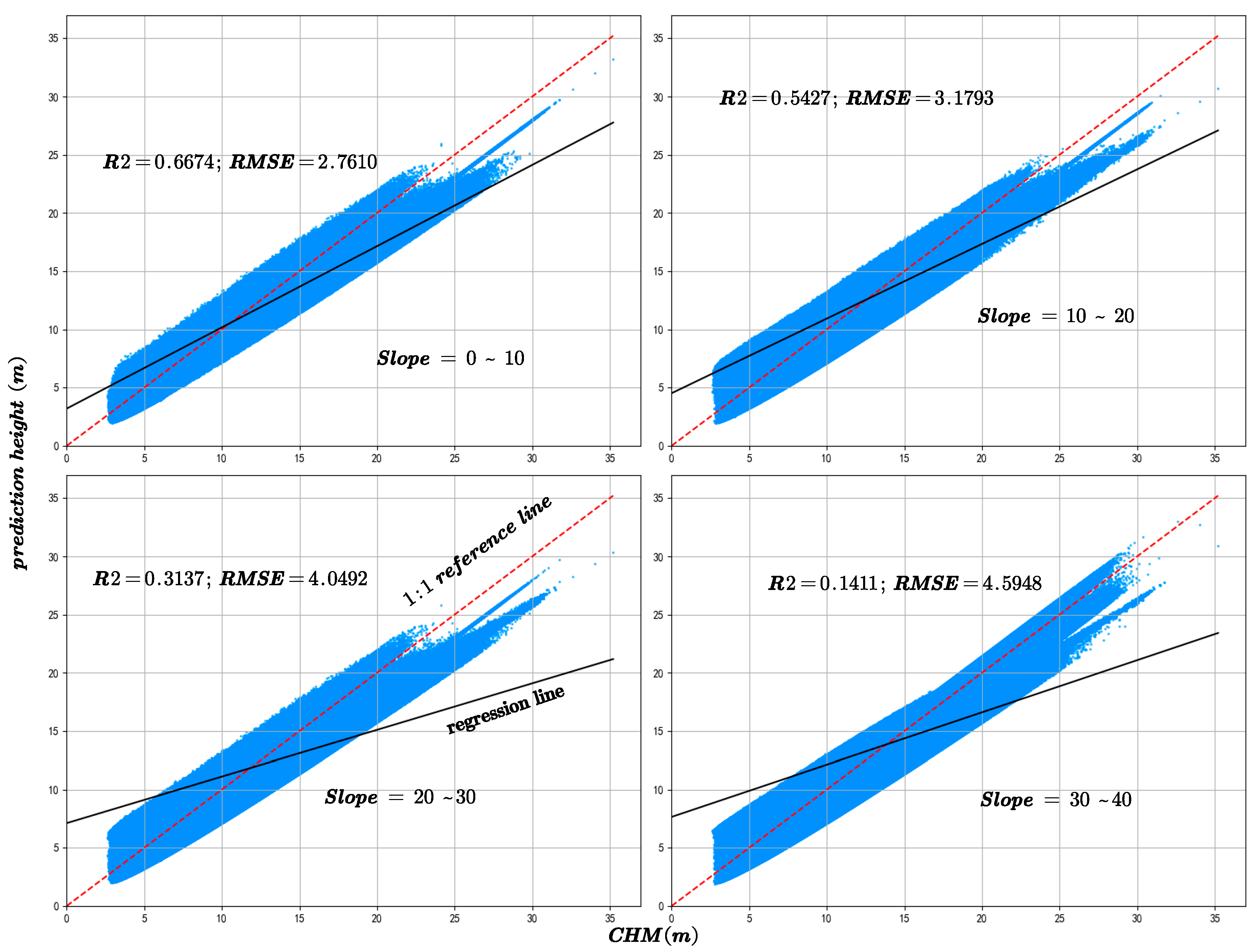
The slope is a critical factor influencing the accuracy of canopy height inversion. In this study, the GEDI data were rigorously filtered to ensure that all footprint centers were located in areas with slopes not exceeding 40°. Based on this criterion, the data were categorized into four slope intervals: 0–10°, 10–20°, 20–30°, and 30–40°, to systematically evaluate the effect of slope on canopy height prediction accuracy. Figure 13 and Figure 14 depict the variation in R2 and RMSE between predicted canopy heights and both GEDI observations and CHM data across these slope intervals.
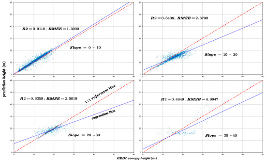
Figure 13.
The model prediction accuracy compared with GEDI canopy height at different slopes.

Figure 14.
The model prediction accuracy compared with the CHM canopy height at different slopes.
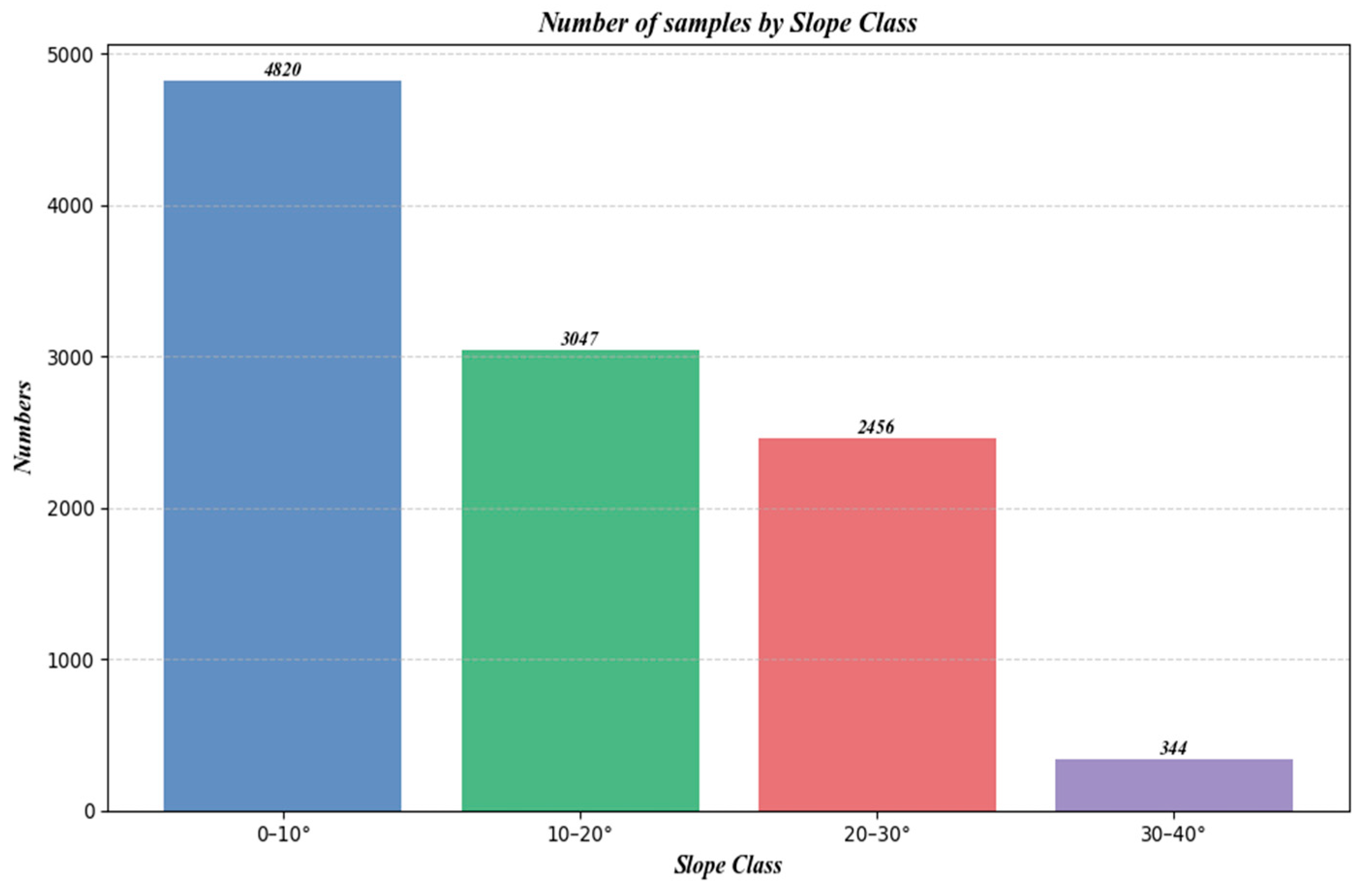
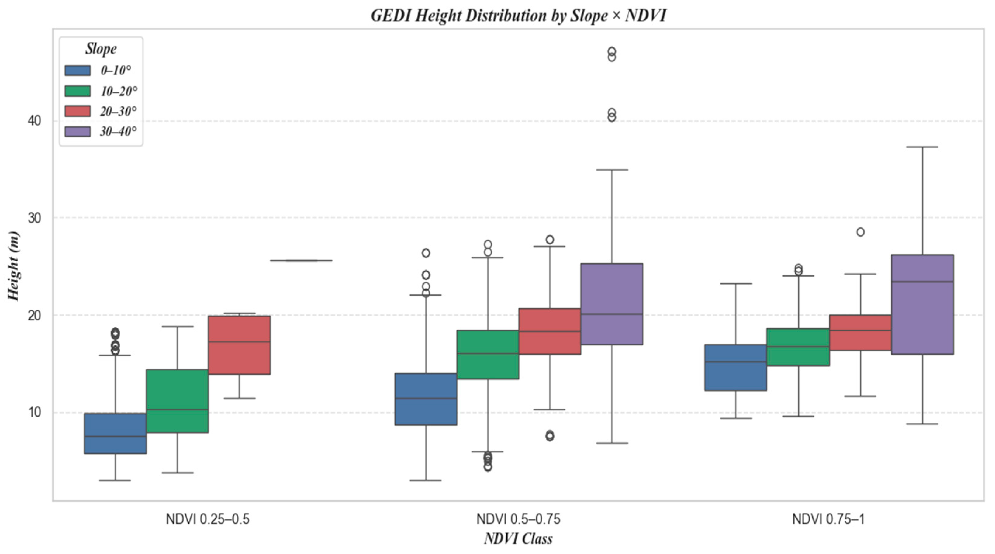
Figure 15 shows the number of samples at different slopes, and Figure 16 is a box plot jointly plotted for different slopes, NDVI, and canopy height.

Figure 15.
Number of samples under different slopes.

Figure 16.
Combined Boxplot of NDVI and Slope Classification.
4.6. Comparison Study
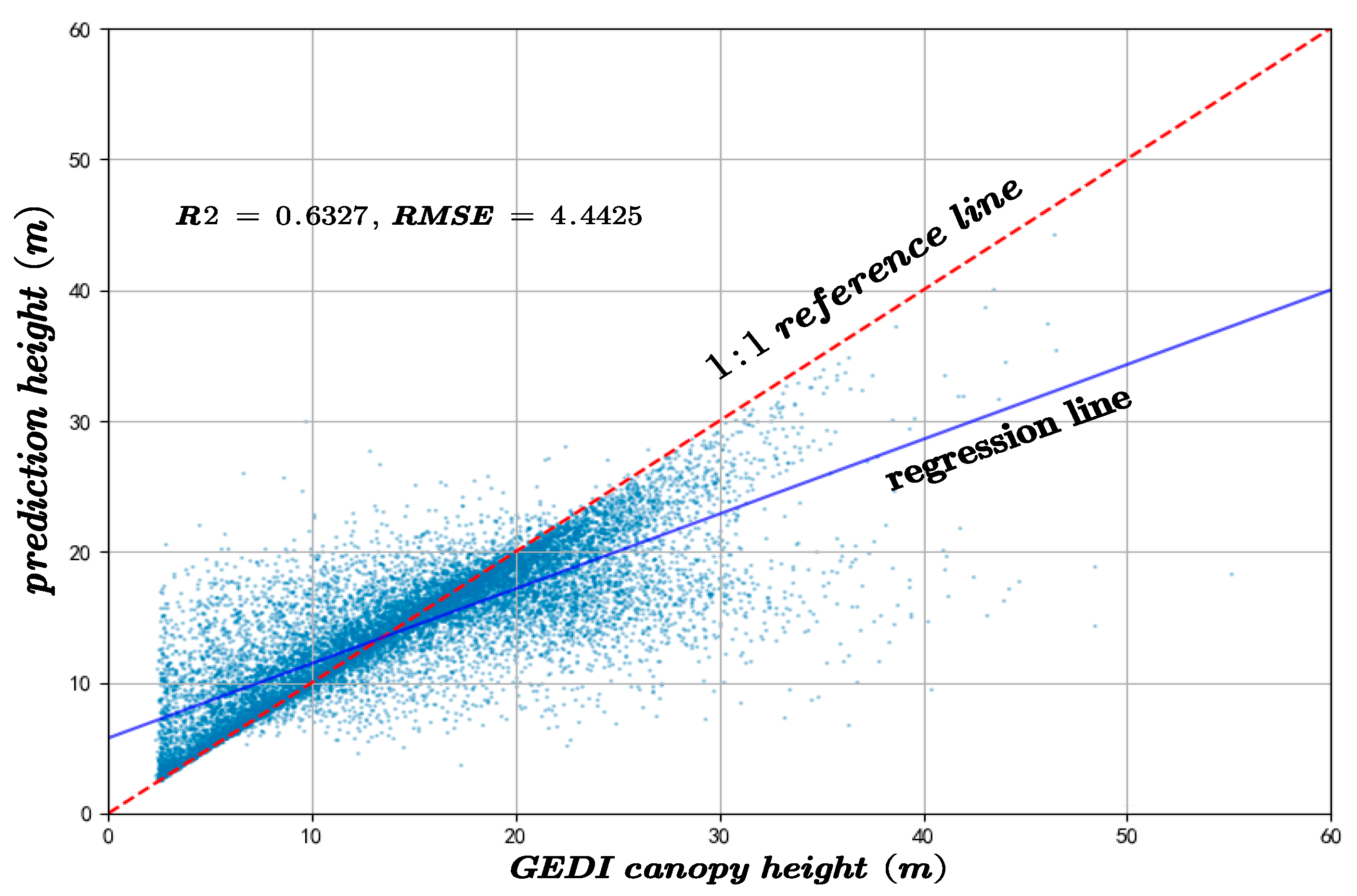
To assess the performance of the proposed method and the resulting canopy height model, a comparative analysis was carried out in relation to the results obtained using the Random Forest (RF) algorithm over the same study area. The predictive performance of both approaches was evaluated using GEDI and CHM validation datasets, with the coefficient of R2 and RMSE serving as the primary evaluation metrics. In canopy height inversion based on GEDI data, the proposed method achieved an R2 of 0.7491 and an RMSE of 2.8025, significantly outperforming the RF model, which yielded an R2 of 0.6327 and an RMSE of 4.4425, as shown in Figure 17.

Figure 17.
The canopy height model inversion accuracy compared to the results of the RF algorithm and the GEDI-derived canopy height.
On the CHM-based validation dataset, the proposed method attained an R2 of 0.5815 and an RMSE of 3.3867, compared to the RF model’s R2 of 0.4167 and RMSE of 3.9279, indicating superior performance in both accuracy and consistency, as shown in Figure 18.
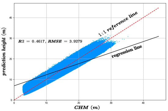
Figure 18.
The canopy height model inversion accuracy compared to the results of the RF algorithm and the CHM-derived canopy height.
As shown in Figure 17 and Figure 18, the comparison of the results obtained using the Random Forest algorithm with those predicted by the proposed method reveals strong evidence that the new approach significantly outperforms the conventional Random Forest in terms of both accuracy and precision. The final canopy height map of the entire Chaling County is presented in Figure 5, which aligns with the actual terrain conditions.
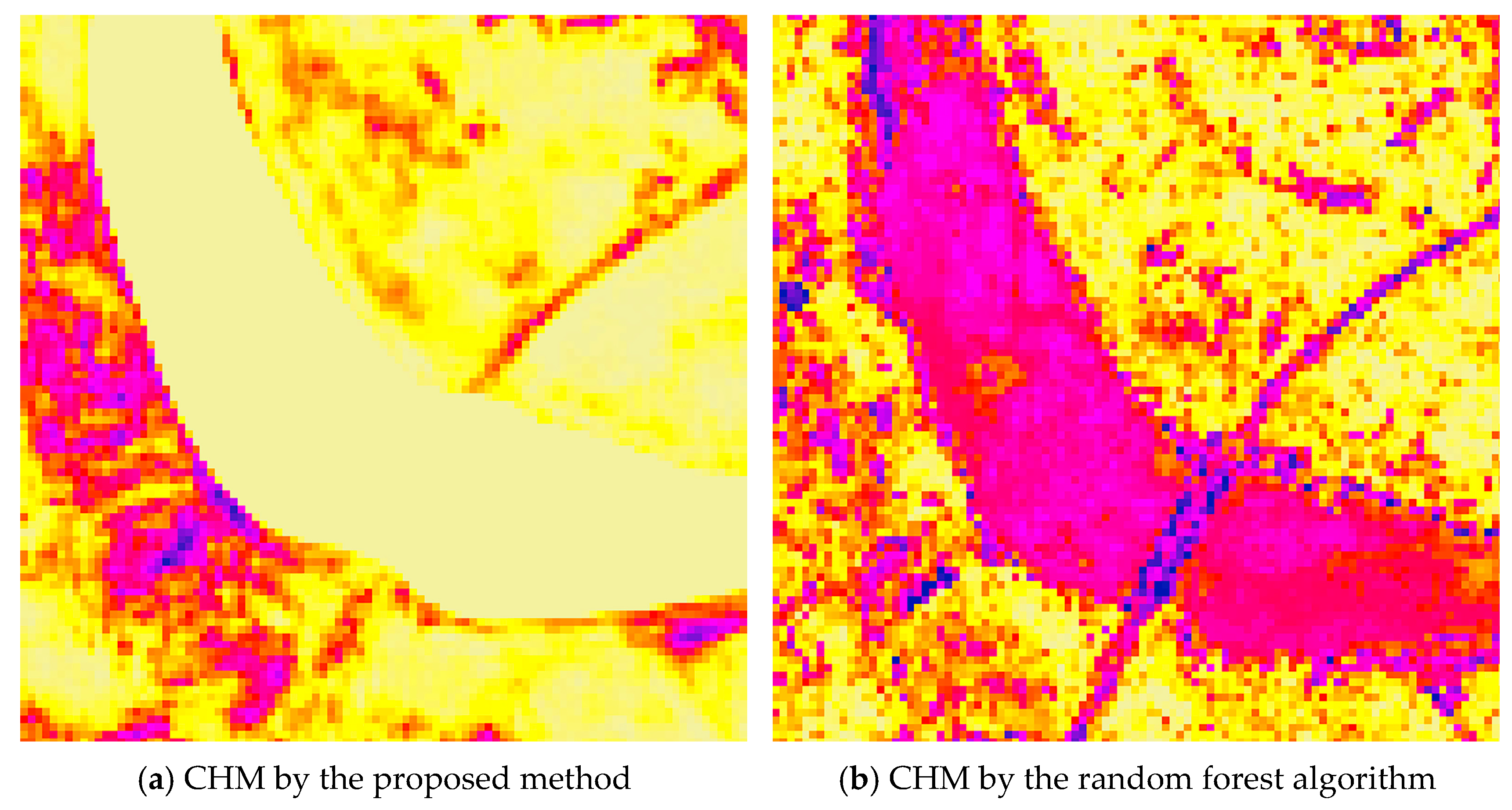
Furthermore, in river regions where the ground surface lacks vegetation and canopy height is expected to be zero, the proposed method accurately predicts zero canopy height values. In contrast, the RF algorithm produces erroneous non-zero height estimates in these areas, as shown in Figure 19.
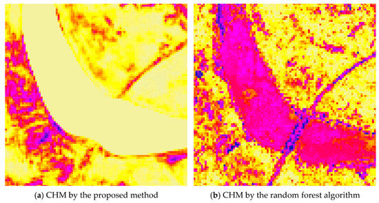
Figure 19.
Part of the canopy height model generated by the proposed method (a) and the canopy height model derived from the random forest algorithm (b), where canopy height increases from yellow (0 m) to purple (>0 m, with the color becoming darker as the canopy height becomes higher).
5. Discussion
5.1. Ablation Experiments
Figure 8 and Figure 9 indicate only a minor difference between U-Net and UNet++ when evaluated on sparse GEDI footprints, whereas UNet++ shows a clear advantage when assessed against continuous CHM data. This disparity stems from the distinct architectural features of the two networks. U-Net’s simple encoder–decoder structure, connected via straightforward skip links, primarily reconstructs spatial information through up-sampling and moderate feature blending. As a result, its outputs tend to be smooth. This inherent smoothness is advantageous for isolated GEDI footprints, as it mitigates the influence of outlier points and keeps point-wise residuals low, producing consistent and visually coherent predictions.
In contrast, UNet++ augments the same backbone with dense skip connections and enhanced multi-scale feature aggregation. This increased capacity allows the network to capture fine-grained height variations present in CHM tiles, reproducing subtle canopy textures and small topographic features more accurately. However, the richer receptive field also makes the network more sensitive to sparse labels, which can occasionally amplify noise around isolated GEDI footprints, leading to slightly higher errors at the point level compared to the smoother U-Net baseline. The main purpose of this study is to predict the canopy height of the region; hence, this paper selects the UNet++ network as the training model.
5.2. Relative Height Factor
As shown in Table 1 in Section 4.1, these findings underscore the importance of selecting an appropriate relative height metric for tree height inversion using GEDI data. Therefore, RH98 was chosen as the optimal indicator for subsequent analyses in this study.
The selection of RH98 is a rational choice based on the physical trade-off within the high signal-to-noise ratio zone: this percentile denotes the height where 98% of the waveform energy becomes accumulated, located precisely in the transition region between the canopy-top return and background noise. It thus provides an optimal balance between suppressing ground-tail artifacts and preserving the upper-canopy signal, resulting in the strongest linear correlation with the reference canopy height model at the Chaling test site (Table 1; highest R2 and lowest RMSE for RH98). However, this preference is not universally applicable. Terrain–structure coupling effects lead to a systematic underestimation of RH98 by approximately −1.2 m on slopes exceeding 30°, due to the elongation of the elliptical footprint, with an associated uncertainty of ±15%. More fundamentally, as an empirical percentile, RH98 lacks a clear physical definition; its optimality varies with forest type, biome, and sub-pixel heterogeneity. Within a 25 m footprint containing both canopy gaps and dense crowns, the metric is biased toward taller vegetation strata, leading to a sub-pixel underestimation ranging from −8% to −12%. Therefore, RH98 is only locally optimal under the specific sensor configuration and environmental conditions of this study; any extrapolation to other regions must involve re-evaluation of percentile sensitivity and terrain-structure coupling errors to avoid conflating statistical performance with mechanistic generalizability.
5.3. Algorithm Factor
Analysis of the results from different algorithms in Table 2 reveals significant variations in accuracy across algorithm configurations. Differences in threshold settings influenced the number of samples included in the validation, which in turn affected inversion accuracy [28]. Therefore, data processed using algorithm group ‘a1’ were selected as the optimal configuration for the study area. After quality filtering, a total of 10,694 GEDI footprints were retained for subsequent analysis.
The designation of algorithm set a1 as “optimal” is based on the rigorous statistical ranking presented in Table 2: under identical quality filtering conditions, it achieves both the highest sample retention and the best validation accuracy (highest R2, lowest RMSE) among the six tested configurations. By applying conservative waveform denoising thresholds and stringent signal-to-noise ratio cut-offs, configuration a1 maximizes the preservation of “clean” canopy-top returns in the undulating terrain and medium-to-high canopy closure conditions characteristic of Chaling County. This enhances the linear relationship between RH98 and the reference canopy height model, resulting in superior inversion performance from a statistical standpoint. However, this advantage is biome-specific: the threshold ensemble of a1 is calibrated for subtropical hilly mixed conifer–broadleaf forests; when applied to tropical rainforests or boreal coniferous stands, its overly aggressive gating may eliminate numerous low-energy yet valid laser pulses, potentially reducing accuracy.
5.4. Vegetation Coverage Factor
Analysis of Figure 10 and Figure 11 reveals that as NDVI values decrease, indicating sparser vegetation cover, the model achieves higher R2 values and lower RMSE, reflecting improved prediction accuracy. Conversely, under denser vegetation cover, prediction accuracy tends to decline. Experimental results indicate that vegetation cover significantly influences canopy height estimation, with most sample points concentrated in low- and moderate-density vegetation areas. This suggests that under high vegetation cover conditions, increased canopy structural complexity combined with limited laser penetration leads to reduced prediction accuracy [29]. Furthermore, the amount of GEDI data used in the training and validation processes also affects predictive performance.
The primary reason lies in the pronounced spatial differentiation of vegetation along the topographic gradient in the study area. Low-elevation gentle slopes (<20°) are predominantly occupied by monoculture plantations of Cunninghamia lanceolata and Pinus massoniana, which exhibit homogeneous canopy structures, simple vertical stratification, and high understory light transmittance. In contrast, moderate to steep slopes (>25°) are mainly covered by natural secondary evergreen broadleaved mixed forests dominated by Schima superba and Cyclobalanopsis glauca. These forests feature dense, multilayer canopies with high Leaf Area Indices (LAI = 5–6) and extensive branch and foliage overlap. Such “high-density–high-complexity” canopy configurations enhance multiple scattering and waveform attenuation, making it difficult to distinguish between canopy and ground returns in GEDI waveforms. Consequently, waveform broadening and retrieval uncertainty increase, resulting in larger RH98 deviations in structurally complex forest stands.
Moreover, the distribution of sample counts across three NDVI classes, as depicted in Figure 12, initially rises and then falls with increasing NDVI values. However, a comparison with Figure 10 and Figure 11 reveals a consistent downward trend in both R2 and RMSE. Additionally, Figure 16 shows that an increase in NDVI affects canopy height at the same slope levels. Consequently, it can be inferred that the physical factor of increased vegetation coverage complicates prediction, thereby affecting the accuracy of the forecasts.
5.5. Slopes Factor
The analysis reveals that the majority of GEDI samples are located in areas with slopes below 30°. As the slope increases, the canopy height estimation accuracy declines significantly, as indicated by decreasing R2 values and increasing RMSE. This finding is consistent with previous studies showing that GEDI waveform signals are more susceptible to topographic distortions in complex terrain, leading to greater uncertainty in canopy height retrieval [30]. For instance, Li et al. [31] reported that when the slope reaches 30°, GEDI height estimation error increases substantially, with RMSE rising to 10.18 m without geolocation correction but decreasing to 6.1 m after correction. Similarly, Kutchartt et al. [32] found in the Alpine region of northern Italy that slope is the most influential factor affecting GEDI canopy height accuracy, followed by canopy cover.
The pronounced slope dependence observed in our study further supports these findings. Model accuracy exhibits a distinct non-linear relationship with slope, showing a sharp decline when slope exceeds approximately 20°. This degradation can be attributed to several slope-induced physical mechanisms affecting GEDI waveform retrieval. First, elliptical footprint elongation on sloping surfaces causes the slant range to be misinterpreted as vertical height, resulting in systematic RH98 overestimations of approximately 1.5–3 m. Second, temporal overlaps between terrain and multilayer canopy returns generate waveform trailing of 5–7 m, obscuring the true ground return and producing mixed canopy–terrain height estimates. Third, multiple scattering between dense vegetation and steep rock surfaces can generate false return peaks, introducing artificial height biases of 2–3 m.
In summary, slope exerts a substantial influence on the accuracy of GEDI canopy height inversion, with the magnitude of this effect increasing as slope steepness increases. These physical factors collectively explain the observed sharp rise in RMSE and concurrent decline in R2 in steep slope areas.
Furthermore, as shown in Figure 15, which categorizes the sample counts by slope, there is an initial increase, followed by a plateau, and then a decrease in sample numbers with increasing slope. Comparing this with Figure 13 and Figure 14, it is evident that despite similar sample counts in the 10–20° and 20–30° slope ranges, there is a significant decline in R2 and RMSE. Additionally, Figure 16 indicates that an increase in slope does influence canopy height under the same NDVI values. Hence, it can be concluded that within these slope ranges, physical factors, specifically the increased difficulty in prediction due to greater slope, are impacting the accuracy of predictions.
5.6. The Ecology and Application Significance of CHM
CHM represents the integrated outcome of numerous ecological processes. Its complex three-dimensional structure creates diverse habitats that support a wide range of species. Forests characterized by greater structural complexity and taller canopies tend to exhibit higher levels of biodiversity. As such, canopy height and its derived structural metrics serve as fundamental indicators for assessing forest ecosystem health. CHM provides critical data support for precision forestry and sustainable forest management. Key structural parameters, such as average stand height, dominant tree height, and timber volume, can be derived rapidly and with high accuracy, reducing reliance on labor-intensive field surveys. By identifying mature forest stands and tall trees that meet harvesting criteria, these maps facilitate selective logging practices that minimize ecological disruption to the broader ecosystem. Furthermore, based on biomass or volume distribution maps, wood yield can be estimated with greater precision, enabling optimized planning of logistics and processing operations.
Biomass estimation and carbon stock assessment rank among the most direct and impactful applications of canopy height maps. A strong correlation exists between tree biomass, particularly above-ground biomass, and structural metrics such as tree height and diameter at breast height. Traditional field-based approaches for establishing these relationships often require tree felling or direct weighing, which are not only time-consuming and labor-intensive but also ecologically disruptive. In contrast, canopy height maps enable a non-destructive alternative: once a “CHM–biomass” model is calibrated, large-scale canopy height data can be efficiently converted into spatially explicit biomass distribution maps. By applying a conversion factor of approximately 0.5 to the biomass estimates, researchers can derive carbon stock values, the key indicators in ecological and climate change studies. Compared to conventional methods, this approach supports large-scale, high-precision, rapid, and non-invasive assessments, significantly enhancing both accuracy and operational efficiency.
CHM has transformed forest research from a two-dimensional perspective into a three-dimensional paradigm, marking a significant advancement in the field. They serve as a central link between forest structure and ecological function, enabling deeper scientific understanding and practical applications. For ecologists, these maps are essential for studying biodiversity, ecosystem succession, and functional dynamics. For climate scientists and policymakers, CHM provides a robust foundation for accurately quantifying the global carbon cycle and assessing the effectiveness of climate change mitigation strategies. For forestry professionals, they offer actionable insights to support efficient, sustainable, and precision-based forest management. The continued development and broad application of CHM hold immense potential for addressing climate change, conserving biodiversity, and ensuring the sustainable management of forest resources.
6. Conclusions
This study focuses on Chaling County, Zhuzhou, Hunan Province, China, where a systematic preprocessing of the GEDI Level 2A product was first performed to extract forest canopy height parameters and retain high-quality LiDAR footprints through rigorous filtering. Subsequently, Sentinel-1 imagery was selected based on ascending orbit information and temporal consistency, while Sentinel-2 images were filtered according to cloud cover and required spectral bands. Finally, the optimized GEDI, Sentinel-1, and Sentinel-2 datasets were jointly input into the developed UNet++ deep-learning network to establish a forest height extrapolation model covering the study area, enabling accurate estimation of canopy height in the entire Chaling County. The model has achieved relatively good performance in the Chaling County area.
The correlations between canopy height percentile metrics (RH96 to RH100) derived from GEDI data, as well as the reference value of canopy height measurements, are comprehensively examined. The results demonstrate that RH98 shows the strongest correlation with the reference data. Furthermore, the study revealed that different processing algorithms have a significant impact on the accuracy of GEDI-derived canopy heights. Through analysis of the correlation between RH98 values processed using six distinct algorithms and the reference measurements, it was found that GEDI data processed with the ‘a1’ algorithm exhibited the highest correlation. These findings suggest that the ‘a1’ algorithm achieves the most accurate canopy height inversion within the scope of this study.
The influences of vegetation coverage and terrain slope on the accuracy of canopy height model inversion are investigated. Vegetation coverage, quantified using NDVI, was categorized into three intervals: 0.25–0.5, 0.5–0.75, and 0.75–1.0. Among these, the intervals of 0.25–0.5 and 0.5–0.75 encompassed the majority of GEDI footprint centers and demonstrated higher canopy height prediction accuracy. This is attributed to the enhanced ability of GEDI signals to penetrate the canopy within these vegetation coverage ranges, thereby capturing more accurate height information. Furthermore, the impact of slope on prediction accuracy was quantitatively assessed by classifying the data into four slope categories. Most GEDI footprint centers were found in areas with slopes below 30°, where canopy height estimation accuracy was significantly better compared to areas with slopes exceeding 30°. These results indicate that terrain slope is a critical factor influencing the accuracy of GEDI-based canopy height inversion. In steep terrain, complex topographic variations disrupt the propagation and reception of GEDI LiDAR signals, thereby reducing the reliability of canopy height estimates.
High-resolution CHM can accurately characterize stand structural attributes and exhibit strong correlations with above-ground vegetation biomass, making them a critical input for regional forest carbon stock estimation and providing reliable data support for carbon cycle research and climate change monitoring. Fine-scale height information also offers practical benefits for forest management and ecological planning, including the design of sustainable harvesting strategies, assessment of forest growth potential, monitoring of post-disturbance (natural or anthropogenic) recovery, and guidance for ecological restoration and protected area governance. In future work, integrating multi-temporal remote sensing observations with topographic and climatic variables will enable dynamic monitoring of forest growth and long-term ecological change. Furthermore, incorporating predictive uncertainty analysis, physics-constrained loss functions, or advanced multimodal data fusion approaches is anticipated to further enhance the precision and robustness of canopy height retrieval. This proposed method not only provides a scientific basis for forest management and carbon stock assessment in Chaling County, but also offers a transferable technical framework for large-scale forest carbon cycle studies and ecosystem service evaluations.
Author Contributions
Conceptualization, X.D. and X.Z.; methodology, X.D. and Y.Y.; software, X.Z.; validation, Z.T., X.D. and X.Z.; formal analysis, X.D. and Y.Y.; investigation, X.Z.; resources, Z.T.; data curation, X.Z.; writing—original draft preparation, X.D.; writing—review and editing, X.Z. and Y.Y.; visualization, X.Z.; supervision, Z.T.; project administration, Z.T.; funding acquisition, X.D. All authors have read and agreed to the published version of the manuscript.
Funding
This research was funded by the Open Topic of Hunan Geospatial Information Engineering and Technology Research Center (Grant No. HNGIET2025001) and the Natural Science Foundation of Hunan Province, China (No. 2024JJ8335).
Data Availability Statement
The original data presented in the study are openly available in Zenodo at https://zenodo.org/records/17103409 (accessed on 12 September 2025) [33].
Conflicts of Interest
The authors declare no conflicts of interest. The authors declare that they have no known competing financial interests or personal relationships that could have appeared to influence the work reported in this paper.
Abbreviations
The following abbreviations are used in this manuscript:
| CHM | Canopy Height Map |
| GEDI | Global Ecosystem Dynamics Investigation |
| MAE | Mean Absolute Error |
| RMSE | Root Mean Square Error |
References
- Han, C.; Chen, N.; Zhang, C.K.; Liu, Y.; Khan, S.; Lu, K.; Li, Y.; Dong, X.; Zhao, C. Sap flow and responses to meteorological about the Larix principis-rupprechtii plantation in Gansu Xinlong mountain, Northwestern China. For. Ecol. Manag. 2019, 451, 117519. [Google Scholar] [CrossRef]
- Harper, A.B.; Powell, T.; Cox, P.M.; House, J.; Huntingford, C.; Lenton, T.M.; Sitch, S.; Burke, E.; Chadburn, S.E.; Collins, W.J.; et al. Land-use emissions play a critical role in land-based mitigation for Paris climate targets. Nat. Commun. 2018, 9, 2938. [Google Scholar] [CrossRef]
- Chen, X.; Jiang, K.; Zhu, Y.; Wang, X.; Yun, T. Individual Tree Crown Segmentation Directly from UAV-Borne LiDAR Data Using the PointNet of Deep Learning. Forests 2021, 2, 131. [Google Scholar] [CrossRef]
- Song, H.X.; You, h.T.; Liu, Y.; Tang, X.; Chen, J.J. Deep Learning-based Segmentation of Citrus Tree Canopy from UAV Multispectral Images. For. Eng. 2023, 39, 140–149. [Google Scholar] [CrossRef]
- Cheng, X. Evaluating ICESat-2 and GEDI with Integrated Landsat-8 and PALSAR-2 for Mapping Tropical Forest Canopy Height. Remote Sens. 2024, 16, 3798. [Google Scholar] [CrossRef]
- Potapov, P.; Li, X.Y.; Hernandez-Serna, A.; Tyukavina, A.; Hansen, M.C.; Kommareddy, A.; Pickens, A.; Turubanova, S.; Tang, H.; Silva, C.E.; et al. Mapping global forest canopy height through integration of GEDI and Landsat data. Remote Sens Environ. 2021, 253, 112165. [Google Scholar] [CrossRef]
- Wang, C.; Song, C.; Schroeder, T.A.; Woodcock, C.E.; Pavelsky, T.M.; Han, Q.; Yao, F. Interpretable Multi-Sensor Fusion of Optical and SAR Data for GEDI-Based Canopy Height Mapping in Southeastern North Carolina. Remote Sens. 2025, 17, 1536. [Google Scholar] [CrossRef]
- Liu, A.; Chen, Y.; Cheng, X. Improving Tropical Forest Canopy Height Mapping by Fusion of Sentinel-1/2 and Bias-Corrected ICESat-2–GEDI Data. Remote Sens. 2025, 17, 1968. [Google Scholar] [CrossRef]
- Tong, Y.; Liu, Z.; Fu, H.; Zhu, J.; Zhao, R.; Xie, Y.; Hu, H.; Li, N.; Fu, S. Forest Canopy Height Estimation Combining Dual-Polarization PolSAR and Spaceborne LiDAR Data. Forests 2024, 15, 1654. [Google Scholar] [CrossRef]
- Lang, N.; Kalischek, N.; Armston, J.; Schindler, K.; Dubayah, R.; Wegner, J.D. Global canopy height regression and uncertainty estimation from GEDI LiDAR waveforms with deep ensembles. Remote Sens. Environ. 2022, 268, 112760. [Google Scholar] [CrossRef]
- Chen, M.; Dong, W.; Yu, H.; Woodhouse, I.; Ryan, C.M.; Liu, H.; Georgiou, S.; Mitchard, E.T.A. Multimodal deep learning for mapping forest dominant height by fusing GEDI with earth observation data. arXiv 2023. [Google Scholar] [CrossRef]
- Cambrin, D.R.; Corley, I.; Garza, P. Depth Any Canopy: Leveraging Depth Foundation Models for Canopy Height Estimation. arXiv 2024, arXiv:2408.04523. [Google Scholar] [CrossRef]
- Lin, X.; Cao, C. Remote Sensing Diagnosis of Forest Canopy Height and Forest Aboveground Biomass Based on ICESat-2 and GEDI. Diss; Aerospace Information Research Institute, Chinese Academy of Sciences: Beijing, China, 2021. [Google Scholar]
- Zhu, X.X. Forest Height Retrieval of China with a Resolution of 30 m Using ICESat-2 and GEDI Data; University of Chinese Academy of Sciences (Institute of Aerospace Information Research, Chinese Academy of Sciences): Beijing, China, 2022. [Google Scholar]
- Fan, G.; Yan, F.; Zeng, X.; Xu, Q.; Wang, R.; Zhang, B.; Zhou, J.; Nan, L.; Wang, J.; Zhang, Z.; et al. First Mapping the Canopy Height of Primeval Forests in the Tallest Tree Area of Asia. arXiv 2024, arXiv:2404.14661. [Google Scholar] [CrossRef]
- Torres, R.; Snoeij, P.; Geudtner, D.; Bibby, D.; Davidson, M.; Attema, E.; Potin, P.; Rommen, B.; Floury, N.; Brown, M.; et al. GMES Sentinel-1 mission. Remote Sens. Environ. 2012, 120, 9–24. [Google Scholar] [CrossRef]
- Main-Knorn, M.; Pflug, B.; Louis, J.; Debaecker, V.; Müller-Wilm, U.; Gascon, F. Sen2Cor for Sentinel-2. In Proceedings of the Image and Signal Processing for Remote Sensing XXIII, Warsaw, Poland, 11–14 September 2017; pp. 37–48. [Google Scholar] [CrossRef]
- Drusch, M.; Del, B.; Carlier, S.; Colin, O.; Fernandez, V.; Gascon, F.; Hoersch, B.; Isola, C.; Laberinti, P.; Martimort, P.; et al. Sentinel-2: ESA’s optical high-resolution mission for GMES operational services. Remote Sens. Environ. 2012, 120, 25–36. [Google Scholar] [CrossRef]
- Gorelick, N.; Hancher, M.; Dixon, M.; Ilyushchenko, S.; Thau, D.; Moore, R. Google Earth Engine: Planetary-scale geospatial analysis for everyone. Remote Sens. Environ. 2017, 202, 18–27. [Google Scholar] [CrossRef]
- Schwartz, M.; Ciais, P.; Ottlé, C.; De Truchis, A.; Vega, C.; Fayad, I.; Brandt, M.; Fensholt, R.; Baghdadi, N.; Morneau, F.; et al. High-resolution canopy height map in the Landes forest (France) based on GEDI, Sentinel-1, and Sentinel-2 data with a deep learning approach. Int. J. Appl. Earth Obs. Geoinf. 2024, 128, 103711. [Google Scholar] [CrossRef]
- Dubayah, R.; Blair, J.B.; Goetz, S.; Fatoyinbo, L.; Hansen, M.; Healey, S.; Hofton, M.; Hurtt, G.; Kellner, J.; Luthcke, S.; et al. The Global Ecosystem Dynamics Investigation: High-resolution laser ranging of the Earth’s forests and topography. Sci. Remote Sens. 2020, 1, 100002. [Google Scholar] [CrossRef]
- Adam, M.; Urbazaev, M.; Dubois, C.; Schmullius, C. Accuracy Assessment of GEDI Terrain Elevation and Canopy Height Estimates in European Temperate Forests: Influence of Environmental and Acquisition Parameters. Remote Sens. 2020, 12, 3948. [Google Scholar] [CrossRef]
- Wang, J.; Shen, X.; Cao, L. Upscaling Forest Canopy Height Estimation Using Waveform-Calibrated GEDI Spaceborne LiDAR and Sentinel-2 Data. Remote Sens. 2024, 16, 2138. [Google Scholar] [CrossRef]
- Farr, T.G.; Rosen, P.A.; Caro, E.; Crippen, R.; Duren, R.; Hensley, S.; Kobrick, M.; Paller, M.; Rodriguez, E.; Roth, L.; et al. The Shuttle Radar Topography Mission. Rev. Geophys. 2007, 45, RG2004. [Google Scholar] [CrossRef]
- Liu, X.; Su, Y.; Hu, T.; Yang, Q.; Liu, B.; Deng, Y.; Tang, H.; Tang, Z.; Fang, J.; Guo, Q. Neural network guided interpolation for mapping canopy height of China’s forests by integrating GEDI and ICESat-2 data. Remote Sens. Environ. 2022, 269, 112844. [Google Scholar] [CrossRef]
- Zhou, Z.; Siddiquee, M.M.R.; Tajbakhsh, N.; Liang, J. UNet++: A Nested U-Net Architecture for Medical Image Segmentation. In Deep Learning in Medical Image Analysis and Multimodal Learning for Clinical Decision Support; Springer: Cham, Germany, 2018; Volume 11045, pp. 3–11. [Google Scholar] [CrossRef] [PubMed] [PubMed Central]
- Guan, L. AdaPlus: Integrating Nesterov Momentum and Precise Stepsize Adjustment on AdamW Basis. In Proceedings of the ICASSP 2024—2024 IEEE International Conference on Acoustics, Speech and Signal Processing (ICASSP), Seoul, Republic of Korea, 14–19 April 2024. [Google Scholar] [CrossRef]
- Liu, L.J.; Wang, C.; Nie, S.; Zhu, X.; Xi, X.; Wang, J. Analysis of the influence of different algorithms of GEDI L2A on the accuracy of ground elevation and forest canopy height. J. Univ. Chin. Acad. Sci. 2022, 39, 502–511. [Google Scholar] [CrossRef]
- Chen, R.; Wang, X.; Liu, X.; Wang, S. Optimizing GEDI Canopy Height Estimation and Analyzing Error Impact Factors Under Highly Complex Terrain and High-Density Vegetation Conditions. Forests 2024, 15, 2024. [Google Scholar] [CrossRef]
- Dong, H.Y. Evaluation and Application of Inversion Accuracy of Understory Terrain and Forest Canopy Height Inversion of Spaceborne LiDAR GEDI Data; Northeast Forestry University: Harbin, China, 2023. [Google Scholar]
- Li, H.; Li, X.; Kato, T.; Hayashi, M.; Fu, J.; Hiroshima, T. Accuracy assessment of GEDI terrain elevation, canopy height, and aboveground biomass density estimates in Japanese artificial forests. Sci. Remote Sens. 2024, 10, 100144. [Google Scholar] [CrossRef]
- Kutchartt, E.; Pedron, M.; Pirotti, F. Assessment of canopy and ground height accuracy from GEDI LiDAR over steep mountain areas. ISPRS Ann. Photogramm. Remote Sens. Spat. Inf. Sci. 2022, 3, 431–438. [Google Scholar] [CrossRef]
- GEDIS1S2. Zenodo. Available online: https://zenodo.org/records/17103409 (accessed on 12 September 2025).
Disclaimer/Publisher’s Note: The statements, opinions and data contained in all publications are solely those of the individual author(s) and contributor(s) and not of MDPI and/or the editor(s). MDPI and/or the editor(s) disclaim responsibility for any injury to people or property resulting from any ideas, methods, instructions or products referred to in the content. |
© 2025 by the authors. Licensee MDPI, Basel, Switzerland. This article is an open access article distributed under the terms and conditions of the Creative Commons Attribution (CC BY) license (https://creativecommons.org/licenses/by/4.0/).

