Nonsmooth Levenberg-Marquardt Type Method for Solving a Class of Stochastic Linear Complementarity Problems with Finitely Many Elements

Abstract

Our purpose of this paper is to solve a class of stochastic linear complementarity problems (SLCP) with finitely many elements. Based on a new stochastic linear complementarity problem function, a new semi-smooth least squares reformulation of the stochastic linear complementarity problem is introduced. For solving the semi-smooth least squares reformulation, we propose a feasible nonsmooth Levenberg–Marquardt-type method. The global convergence properties of the nonsmooth Levenberg–Marquardt-type method are also presented. Finally, the related numerical results illustrate that the proposed method is efficient for the related refinery production problem and the large-scale stochastic linear complementarity problems.

1. Introduction

Suppose $(\Omega ,F,P)$ is a probability space with $\Omega \subseteq {\Re }^n$ and P is a known probability distribution. A stochastic linear complementarity problem takes the form:

$$x\ge 0,M\left(\omega \right)x+q\left(\omega \right)\ge 0,x^T[M\left(\omega \right)x+q\left(\omega \right)]=0a.e.\omega \in \Omega ,$$

(1)

where $\Omega \subseteq {\Re }^n$ is the underlying sample space, for given probability distribution P and ∀ $\omega \in \Omega$, $M\left(\omega \right)\in {\Re }^{n\times n}$ and $q\left(\omega \right)\in {\Re }^n$. (1) is denoted as SLCP $\left(M\right(·),q(·\left)\right)$ or SLCP; see [1,2,3,4]. If Ω has only one element, (1) is the standard linear complementarity problem (LCP), which has been studied in [5,6].

Generally, there is no x satisfying (1) for all $\omega \in \Omega$. In order to obtain a reasonable solution of Problem (1), several types of models have been proposed (one can see [1,2,3,4,7,8,9,10,11,12,13,14]). One of them is the expected value (EV) method (see [1]). The EV model is to find a vector $x\in {\Re }^n$, such that:

$$0\le x\perp \overline{M}x+\overline{q}\ge 0,$$

(2)

where $\overline{M}=E\left[M\left(\omega \right)\right]$, $\overline{q}=E\left[q\left(\omega \right)\right]$, and $E[.]$ is the mathematical expectation. Another is the expected residual minimization (ERM) method (see [2]). The ERM model is to find a vector $x\in {\Re }_{+}^n$ that minimizes the expected residual function:

$$\underset{x\ge 0}{min}{\displaystyle \sum _{i=1}^n}E{\left[\phi (x_i,M_i\left(\omega \right)x+q_i\left(\omega \right))\right]}^2,$$

where $M_i\left(\omega \right)(i=1,\cdots ,n)$ is the i-th line of random matrix $M\left(\omega \right)$ and φ satisfies:

$$\phi (a,b)=0⟺a\ge 0,b\ge 0,ab=0.$$

In addition to [1,2], Luo and Lin first considered a quasi-Monte Carlo method in [8,9]; they proved that the ERM method is convergent under mild conditions and studied the properties of the ERM problems. In [10], Chen, Zhang and Fukushima considered SLCP including the expectation of matrix is positive semi-definite. Under the condition of a new error bound, they use the ERM formulation to solve the SLCP. In [11], they also studied the ERM formulation, where the involved function is a stochastic $R_0$ function. In [12], Zhou and Caccetta put forward a new model of the stochastic linear complementarity problem with only finitely many elements. A feasible semi-smooth Newton method was also given. In [14], Ma also considered a feasible semi-smooth Gauss–Newton method for solving this new stochastic linear complementarity problem. The stochastic linear complementarity problem with only finitely many elements is to find a vector $x\in {\Re }^n$, such that:

$$x\ge 0,M\left({\omega }_i\right)x+q\left({\omega }_i\right)\ge 0,x^T[M\left({\omega }_i\right)x+q\left({\omega }_i\right)]=0i=1,\cdots ,m,m>1,$$

(3)

where $\Omega =\{{\omega }_1,{\omega }_2,\cdots ,{\omega }_m\}.$ Denote:

$$\overline{M}={\displaystyle \sum _{i=1}^m}{p}_{i}M\left({\omega }_i\right),\overline{q}={\displaystyle \sum _{i=1}^m}{p}_{i}q\left({\omega }_i\right),$$

where $p_i=P({\omega }_i\in \Omega )>0,i=1,\cdots ,m$. Then, (3) is equivalent to:

$$x\ge 0,\overline{M}x+\overline{q}\ge 0,x^T(\overline{M}x+\overline{q})=0,$$

(4)

$$M\left({\omega }_i\right)x+q\left({\omega }_i\right)\ge 0,i=1,\cdots ,m.$$

(5)

where (4) is called the linear complementarity problem.

As we all know, in [15,16,17,18,19,20,21,22,23,24,25,26,27,28,29], many methods were given for solving the nonlinear complementarity problem (NCP) and linear complementarity problem (LCP), such as Kanzow and Petra, who presented a nonsmooth least squares reformulation of (4) in [15]. They defined $\Phi :{\Re }^n\to {\Re }^{2n}$ as:

$$\Phi \left(x\right)=\left(\begin{array}{c}\lambda {\varphi }_{FB}(x_i,{\overline{M}}_{i}x+{\overline{q}}_i),i=1\cdots n\\ ⋮\\ (1-\lambda ){\varphi }_{+}(x_i,{\overline{M}}_{i}x+{\overline{q}}_i),i=1\cdots n\end{array}\right),$$

where $\lambda \in (0,1)$, ${\varphi }_{FB}(a,b)={\parallel (a,b)\parallel }_2-(a+b)$, ${\varphi }_{+}(a,b)=a_{+}{b}_{+}$, $z_{+}=max\{0,z\}$ for $z\in \Re$. This least squares formulation can gave a faster reduction of the complementarity gap $x^T(\overline{M}x+\overline{q})$.

On the other hand, the authors of [16,18,19] studied the generalized Fischer–Burmeister function, i.e., ${\varphi }_p:{\Re }^n\to \Re$ given by ${\varphi }_p(a,b)={\parallel (a,b)\parallel }_p-(a+b)$ $(p\in (1,+\infty \left)\right)$. Additionally, their research work has shown that this class of functions enjoys some favorable properties as other NCP-functions. The given numerical results for the test problems from mixed complementarity problem library (MCPLIB) have shown that the descent method has better performance when p decreases in $(1,+\infty )$.

The main motivation of this paper is to use the advantages of [12,15,16,18,19] to solve the stochastic linear complementary problem denoted as (3). Firstly, we put forward a new robust reformulation of the complementarity Problem (3). Then, based on the new robust reformulation, we propose a feasible nonsmooth Levenberg–Marquardt-type method to solve (3). The numerical results in Section 4 showed that the given Method 1 is efficient for the related refinery production problem and the large-scale stochastic linear complementarity problems. We also make a comparison with Method 1 and the scaled trust region method (STRM) in [20]; preliminary numerical experiments showed that the numerical results of Method 1 are as good as the numerical results of the STRM method. Additionally, it generates less iterations in contrast to the STRM method. Additionally, we also make a comparison with Method 1 and the method in [13] for solving the related refinery production problem. The preliminary numerical experiments also indicate that Method 1 is quite robust. In other words, Method 1 has the following advantages.

• Faster reduction of the complementarity gap $x^T(\overline{M}x+\overline{q})$.
• Flexible NCP functions ${\varphi }_p$.
• Randomly-chosen initial points and less calculation.

Now is the time to give a new reformulation of (4); the new reformulation of (4) is:

$${\varphi }_n\left(x\right)=\left(\begin{array}{c}\lambda {\varphi }_p(x_i,{\overline{M}}_{i}x+{\overline{q}}_i),i=1\cdots n\\ ⋮\\ (1-\lambda ){\varphi }_{+}(x_i,{\overline{M}}_{i}x+{\overline{q}}_i),i=1\cdots n\end{array}\right),$$

(6)

where ${\varphi }_n:{\Re }^n\to {\Re }^{2n}$, $\lambda \in (0,1)$. Then, x is a solution of (4) ⟺${\varphi }_n\left(x\right)=0$. Additionally, solving (4) is also equivalent to finding a solution of the unconstrained optimization problem:

$$\underset{x\in {\Re }^n}{min}\Psi \left(x\right),$$

(7)

where:

$$\Psi \left(x\right)=\frac{1}{2}{\parallel {\varphi }_n\left(x\right)\parallel }^2.$$

(8)

Then, (4) and (5) can be rewritten as:

$$F(x,y)=0,y\ge 0,\left(9\right)$$

(9)

where:

$$F(x,y)=\left(\begin{array}{c}{\varphi }_n\left(x\right)\\ M\left({\omega }_1\right)x+q\left({\omega }_1\right)-y_1\\ M\left({\omega }_2\right)x+q\left({\omega }_2\right)-y_2\\ ⋮\\ M\left({\omega }_m\right)x+q\left({\omega }_m\right)-y_m\end{array}\right).$$

Additionally, $y={[y_1^T,y_2^T,\dots ,y_m^T]}^T\in {\Re }^{mn}$ is a slack variable with $y_i\in {\Re }^n,i=1,2,\dots ,m$. Then, we know that $F(x,y)=0$ has $(m+2)n$ equations with $(m+1)n$ variables.

The remainder of this paper is organized as follows. In Section 2, we review some background definitions and some useful properties. In Section 3, we define a merit function $\theta \left(z\right)=\frac{1}{2}{\parallel F\left(z\right)\parallel }^2$ and give a feasible nonsmooth Levenberg–Marquardt-type method. Some discussions about this method are also given. In Section 4, the numerical results indicate that the given method is efficient for solving stochastic linear complementarity problems, such as the related refinery production problem and the large-scale stochastic linear complementarity problems.

2. Preliminaries

In this section, we give some related definitions and some properties; some of them can be found in [6,14,15,19,20,21,22,23]; some of them are given for the first time.

Let $G:{\Re }^m⟶{\Re }^n$ be a locally-Lipschitzian function. The B-subdifferential of G at x is:

$${\partial }_{B}G\left(x\right)=\{V\in {\Re }^{m\times n}|\exists \left\{x_k\right\}\subseteq D_G:\left\{x_k\right\}\to x,G^{\prime }\left(x_k\right)\to V\},$$

where $D_G$ is the differentiable points set and $G^{\prime }\left(x\right)$ is the Jacobian of G at a point $x\in {\Re }^n$.

The Clarke generalized Jacobian of G is defined as:

$$\partial G\left(x\right)=conv\{V\in {\Re }^{m\times n}|\exists \left\{x_k\right\}\subseteq D_G:\left\{x_k\right\}\to x,G^{\prime }\left(x_k\right)\to V\}.$$

Furthermore,

$${\partial }_{C}G{\left(x\right)}^T=\partial G_1\left(x\right)\times \cdots \times \partial G_m\left(x\right)$$

denotes the C-subdifferential of G at x.

If

$$\underset{V\in \partial G(x+t{h}^{\prime }),h^{\prime }\to h,t\to 0^{+}}{lim}V{h}^{\prime }$$

exists for any $h\in {\Re }^m$, we call G is semi-smooth at x.

Definition 1.

([6]) Matrix $M\in {\Re }^{n\times n}$ is called a:

(a) 

$P_0$-matrix, if each of its principal minors is nonnegative.

(b) 

P-matrix, if each of its principal minors is positive.

Definition 2.

([23]) Let $G:{\Re }^n⟶{\Re }^n$; the following statements are given:

(a) 

We call G monotone, if ${(x-y)}^T(G\left(x\right)-G\left(y\right))\ge 0$, for $x,y\in {\Re }^n$.

(b) 

G is a $P_0$ function, if:

$$\underset{1\le i\le n}{max}(x_i-y_i)(G_i\left(x\right)-G_i\left(y\right))\ge 0$$

for all $x,y\in {\Re }^n$, $x\ne y$ and $x_i\ne y_i$.

Proposition 1.

([6]) $M\in {\Re }^{n\times n}$ is a $P_0$-matrix ⟺ $\forall x\ne 0$, $x_i{\left(Mx\right)}_i\ge 0,x_i\ne 0$.

Proposition 2.

([21]) Suppose G is a locally-Lipschitzian function and strongly semi-smooth at x. Additionally, it is also directionally differentiable in a neighborhood of x; we get:

$$\underset{h\to 0,H\in \partial G(x+h)}{lim}\frac{\parallel G(x+h)-G\left(x\right)-Hh\parallel }{{\parallel h\parallel }^2}<\infty .$$

Definition 3.

We call $x^{*}$ an R-regular solution of the complementarity problem $x\ge 0,G\left(x\right)\ge 0$, $x^{T}G\left(x\right)=0$, if $G^{\prime }{\left(x^{*}\right)}_{\alpha \alpha }$ is nonsingular and $G^{\prime }{\left(x^{*}\right)}_{\beta \beta }-G^{\prime }{\left(x^{*}\right)}_{\beta \alpha }{G}^{\prime }{\left(x^{*}\right)}_{\alpha \alpha }^{-1}{G}^{\prime }{\left(x^{*}\right)}_{\alpha \beta }$ is a P-matrix, where $\alpha =\left\{i\right|x_i^{*}>0,G_i\left(x^{*}\right)=0\}$, $\beta =\left\{i\right|x_i^{*}=0,G_i\left(x^{*}\right)=0\}$, $\gamma =\left\{i\right|x_i^{*}=0,G_i\left(x^{*}\right)>0\}$.

Proposition 3.

([15]) The generalized gradient of ${\varphi }_P$ at a point $(a,b)$ is defined as:

$$\partial \varphi (a,b)=(g_a,g_b)=\left\{\begin{array}{c}(\frac{{sgn\left(a\right)\left|a\right|}^{p-1}}{{\parallel (a,b)\parallel }_p^{p-1}}-1,\frac{{sgn\left(b\right)\left|b\right|}^{p-1}}{{\parallel (a,b)\parallel }_p^{p-1}}-1),(a,b)\ne (0,0)\\ (ϵ-1,\zeta -1),(a,b)=(0,0)\end{array}\right.,$$

where ${\parallel (ϵ,\zeta )\parallel }_P\le 1$. The generalized gradient of ${\varphi }_{+}$ at a point $(a,b)$ is defined as $\partial {\varphi }_{+}(a,b)=\left\{(b_{+}\partial a_{+},a_{+}\partial b_{+})\right\}$, where:

$$\partial Z_{+}=\left\{\begin{array}{c}1,Z>0\\ 0,Z<0\end{array}\right.,$$

$\partial Z_{+}=[0,1]$, if $Z=0$.

Definition 4.

When $x^{*}>0,\overline{M}{x}^{*}+\overline{q}>0$, then (4) is called strictly feasible at $x^{*}$.

Proposition 4.

([15]) All $H\in {\partial }_C\varphi \left(x\right)$ can be defined as:

$$\left(\begin{array}{c}\lambda H_1\\ (1-\lambda )H_2\end{array}\right),$$

where $H_1\subseteq diag\left\{a_i\left(x\right)\right\}+diag\left\{b_i\left(x\right)\right\}\overline{M}$, $H_2\subseteq diag\left\{\widetilde{a_i}\left(x\right)\right\}+diag\left\{\widetilde{b_i}\left(x\right)\right\}\overline{M}$, $(a_i\left(x\right),b_i\left(x\right))\in \partial {\varphi }_P(x_i,{(\overline{M}x+\overline{q})}_i)$, $(\widetilde{a_i}\left(x\right),\widetilde{b_i}\left(x\right))\in \partial {\varphi }_{+}(x_i,{(\overline{M}x+\overline{q})}_i)$, $\partial {\varphi }_P(x_i,{(\overline{M}x+\overline{q})}_i)$ and $\partial {\varphi }_{+}(x_i,{(\overline{M}x+\overline{q})}_i)$ are given in Proposition 3.

Proposition 5.

([15]) Suppose that (4) is R-regular at $x^{*}$, then, all elements of ${\partial }_C\varphi \left(x^{*}\right)$ have full rank.

For any $(x,y)\in {\Re }^{(m+1)n},$ we know that:

$${\partial }_{C}F(x,y)=\left\{\left(\begin{array}{c}{V}_{{\varphi }_n}00\cdots 0\\ M\left({\omega }_1\right)-I0\cdots 0\\ M\left({\omega }_2\right)0-I\cdots 0\\ ⋮\\ M\left({\omega }_m\right)00\cdots -I\end{array}\right):V_{{\varphi }_n}\in {\partial }_C{\varphi }_n\left(x\right)\right\},$$

where I is the $n\times n$ identity matrix. Hence, by Proposition 5, we know that the following proposition is set up.

Proposition 6.

Suppose (4) is R-regular at $x^{*}$ and $(x^{*},y^{*})$ is a solution of (9). Then, all $V\in {\partial }_{C}F(x^{*},y^{*})$ are nonsingular.

Proposition 7.

If (4) is R-regular at a solution $x^{*}$, then, there exits $\alpha >0,\beta >0$, such that $\parallel {\left(H^{T}H\right)}^{-1}\parallel \le \beta$ for all $x^{*}\in {\Re }^n$ with $\parallel x-x^{*}\parallel \le \alpha ,$ where $H\in {\partial }_C\varphi \left(x\right)$.

Proof of Proposition 7.

The proof is similar to the ([15], Lemma 2.5) and therefore omitted here. ☐

In the following part of this paper, we rewrite Ψ as:

$$\Psi \left(x\right)=\frac{1}{2}{\parallel {\varphi }_n\left(x\right)\parallel }^2={\displaystyle \sum _{i=1}^n}\psi (x_i,{(\overline{M}x+\overline{q})}_i),$$

where $\psi :{\Re }^2\to \Re$ is defined as:

$$\psi (a,b)=\frac{1}{2}{\lambda }^2{\varphi }_P^2(a,b)+\frac{1}{2}{(1-\lambda )}^2{a}_{+}^2{b}_{+}^2.$$

Proposition 8.

The function $\Psi :{\Re }^n\to \Re$ defined in (8) satisfies:

(a) 

$\nabla \Psi \left(x\right)=V^T{\varphi }_n\left(x\right)$, for any $V\in {\partial }_C{\varphi }_n\left(x\right)$.

(b) 

If $\nabla \Psi \left(x^{*}\right)=0$ and $\overline{M}$ is a $P_0$ matrix, we know that $x^{*}$ is a solution of (4).

(c) 

If (4) is strictly feasible and $x⟼\overline{M}x+\overline{q}$ is monotone, then $L\left(c\right)=\{x\in {\Re }^n|\Psi \left(x\right)\le c\}$ are compact for all $c\in \Re$.

Proof of Proposition 8.

The proof is similar to the one of ([15], Theorem 2.7), so we skip the details here. ☐

3. The Feasible Nonsmooth Levenberg–Marquardt-Type Method and Its Convergence Analysis

In this section, we define a merit function $\theta \left(z\right)=\frac{1}{2}{\parallel F\left(z\right)\parallel }^2$ and give a feasible nonsmooth Levenberg–Marquardt-type method. At the same time, we also give some discussions about this method.

Let $z=(x,y)\in {\Re }^{(m+1)n}$; define a merit function of (9) by:

$$\theta \left(z\right)=\frac{1}{2}{\parallel F\left(z\right)\parallel }^2.$$

If (3) has a solution, then solving (9) is equivalent to finding a global solution of the following constrained optimization problem:

$$min\theta \left(z\right)$$

$$s.t.z\ge 0.$$

(10)

If z satisfies:

$$P_Z[z-\nabla \theta \left(z\right)]-z=0,$$

(11)

where $P_Z(·)$ is an orthogonal projection operator onto $Z=\{z\in {\Re }^{(m+1)n}|z\ge 0\}$, then z is a stationary point of (10). Obviously, (11) is equivalent to the following problem:

$$\nabla \theta \left(z\right)\ge 0,z\ge 0,z^T\nabla \theta \left(z\right)=0.$$

(12)

Lemma 1.

([14]) Let $P_Z(·)$ be an orthogonal projection operator onto $Z=\{z\in {\Re }^{(m+1)n}|z\ge 0\}$. The following statements hold:

(a) 

$\parallel P_Z\left(x\right)-P_Z\left(y\right)\parallel \le \parallel x-y\parallel$ for all $x,y\in {\Re }^{(m+1)n}$.

(b) 

For any $y\in Z$, ${(P_Z\left(x\right)-x)}^T(P_Z\left(x\right)-y)\le 0$ for all $x\in {\Re }^{(m+1)n}$.

Proposition 9.

([15]) The merit function θ has the following properties.

(a) 

$\theta \left(z\right)$ is continuously differentiable on ${\Re }^{(m+1)n}$ with $\nabla \theta \left(z\right)=H^{T}F\left(z\right)$ for any $H\in {\partial }_{C}F\left(z\right)$.

(b) 

Assume $x⟼\overline{M}x+\overline{q}$ is monotone, if $LCP(\overline{M},\overline{q})$ has a strictly feasible solution, then for all $c>0,$ we know that the level set:

$$L\left(c\right)=\{z\in {\Re }^{(m+1)n}|\theta \left(z\right)\le c\}$$

is bounded.

For some monotone stochastic linear complementarity problems, the stationary points of (10) may not be a solution. Such as let $n=1$, $m=2$, $\Omega =\{{\omega }_1,{\omega }_2\}=\{0,1\}$, $M\left({\omega }_1\right)=M\left({\omega }_2\right)=1$, $q\left({\omega }_1\right)=1$, $q\left({\omega }_2\right)=-1$, and $p_i=P\{{\omega }_i\in \Omega \}=0.5,i=1,2$, (see [12] ).

By simple computation, we know that the above of problem is a monotone SLCP, obviously; all points $x\ge 1$ are feasible, but this example has no solution. By:

$$F(x,y_1,y_2)=\left(\begin{array}{c}\lambda {\left(2x^p\right)}^{\frac{1}{p}}-2\left|x\right|\\ (1-\lambda ){\left(x_{+}\right)}^2\\ x+1-y_1\\ x-1-y_2\end{array}\right),$$

and (0, 1, 0) is a stationary point of the constraint optimization problem:

$$min\frac{1}{2}{\parallel F(x,y_1,y_2)\parallel }^2$$

$$s.t.x\ge 0,y_1\ge 0,y_2\ge 0.$$

However, $x=0$ is not a solution of this example.

Therefore, in the following proposition, we give some conditions for (3).

Proposition 10.

For monotone Problem (3), let $z^{*}=(x^{*},y^{*})$ be a stationary point of (10). If $M\left({\omega }_i\right)x^{*}+q\left({\omega }_i\right)-y_i^{*}=0,i=1,2,\dots m,$ then $x^{*}$ is a solution of (3).

Proof of Proposition 10.

Assuming that $z^{*}=(x^{*},y^{*})$ is a stationary point of (10), if $M\left({\omega }_i\right)x^{*}+q\left({\omega }_i\right)-y_i^{*}=0,i=1,2,\dots m,$ by (12), we know that $x^{*}$ is the stationary point of the following problem:

$$min\{\Psi (x\left)\right|x\ge 0\}.$$

Similar to the proof of Theorem 3 in [24], it can be shown that $x^{*}$ is a solution of $\Psi \left(x\right)=0.$ Thus, $x^{*}$ is a solution of (3). ☐

Now, we present the feasible nonsmooth Levenberg–Marquardt-type method for solving (3).

Method 1.

Choose $z_0\in Z,\sigma \in (0,\frac{1}{2}),\epsilon \ge 0,\beta ,\gamma \in (0,1)$. Set $k=0$.

Step 1. 

If $\left|\theta \right(z_k\left)\right|\le \epsilon$, stop.

Step 2. 

Choose $H_k\in {\partial }_{C}F\left(z_k\right)$, ${\nu }_k=\parallel F\left(z_k\right)\parallel >0$, and find the solution $d_k$ of the equations:

$$(H_k^T{H}_k+{\nu }_{k}I)d=-\nabla \theta \left(z_k\right).$$

(13)

Step 3. 

If

$$\parallel F\left(P_Z(z_k+d_k)\right)\parallel \le \gamma \parallel F\left(z_k\right)\parallel ,$$

then set $z_{k+1}=P_Z(z_k+d_k)$, $k=k+1,$ and go to Step 1; otherwise, go to Step 4.

Step 4. 

Compute $t_k=max\left\{{\beta }^l\right|l=0,1,2\cdots \}$, such that:

$$\theta \left(z_k\left(t_k\right)\right)\le \theta \left(z_k\right)+\sigma \nabla \theta {\left(z_k\right)}^T(z_k\left(t_k\right)-z_k),$$

where $z_k\left(t_k\right)=P_Z[z_k-t_k\nabla \theta \left(z_k\right)]$. Set $z_{k+1}=z_k\left(t_k\right)$, $k=k+1$, and go to Step 1.

We now investigate the convergence properties of Method 1. In the following sections, we assume that Method 1 generates an infinite sequence.

Theorem 1.

Method 1 is well defined for a monotone SLCP (3). If Method 1 does not stop at a stationary point in finite steps, an infinite sequence $\left\{z_k\right\}$ is generated with $\left\{z_k\right\}\subset Z,$ and any accumulation point of the sequence $\left\{z_k\right\}$ is a stationary point of θ.

Proof of Theorem 1.

Method 1 is well defined for the reason of ${\nu }_k>0$, and $d_k$ is always a descent direction for θ. Now, we consider the following two situations respectively.

(I)

If the direction $d_k$ is accepted by an infinite number of times in Step 3 of Method 1, we get:

$$z_{k+1}=P_Z[z_k+d_k]\in Z.$$

Since $\nabla \theta \left(z_k\right)\ne 0$ implies $d_k\ne 0,$ we have:

$$\nabla \theta {\left(z_k\right)}^T{d}_k=-{\left((H_k^T{H}_k+{\nu }_{k}I)d_k\right)}^T{d}_k<0.$$

From [17], we know that $\left\{\theta \left(z_k\right)\right\}$ is monotonically decreasing. Obviously, this implies that the sequence $\{\parallel F\left(z_k\right)\parallel \}$ is also monotonically decreasing. Since $\parallel F\left(P_Z(z_k+d_k)\right)\parallel \le \gamma \parallel F\left(z_k\right)\parallel$ is accepted by an infinite number of times in view of our assumptions, therefore we get $\parallel F\left(z_k\right)\parallel \to 0$ for $k\to \infty$ by $\gamma \in (0,1).$ This means that any accumulation point of $\left\{z_k\right\}$ is the solution of (10); therefore, it is also a stationary point of $\theta$.

(II)

This case is the negation of Case (I); without loss of generality, we assume that the Levenberg–Marquardt direction is never accepted. If the direction $P_Z[z_k-t_k\nabla \theta \left(z_k\right)]-z_k$ is accepted by an infinite number of times in Step 4 of Method 1, we have:

$$z_{k+1}=P_Z[z_k-t_k\nabla \theta \left(z_k\right)]\in Z.$$

By (b) in Lemma 1, taking $x:=z_k-t_k\nabla \theta \left(z_k\right)$, $y:=z_k$, we get:

$$\begin{array}{ccc}\hfill 0& \ge & {[P_Z(z_k-t_k\nabla \theta \left(z_k\right))-(z_k-t_k\nabla \theta \left(z_k\right))]}^T[P_Z(z_k-t_k\nabla \theta \left(z_k\right))-z_k]\hfill \\ & =& {[P_Z(z_k-t_k\nabla \theta \left(z_k\right))-z_k+t_k\nabla \theta \left(z_k\right)]}^T[P_Z(z_k-t_k\nabla \theta \left(z_k\right))-z_k]\hfill \\ & =& {(P_Z(z_k-t_k\nabla \theta \left(z_k\right))-z_k)}^2+t_k\nabla \theta {\left(z_k\right)}^T[P_Z(z_k-t_k\nabla \theta \left(z_k\right))-z_k]\hfill \end{array}$$

that is,

$$\nabla \theta {\left(z_k\right)}^T[P_Z(z_k-t_k\nabla \theta \left(z_k\right))-z_k]\le -\frac{{(P_Z(z_k-t_k\nabla \theta \left(z_k\right))-z_k)}^2}{t_k}\le 0,$$

where $t_k=max\left\{{\beta }^l\right|l=0,1,2\cdots \}$ with $\beta \in (0,1)$. By the Armijo line search properties, we know that any accumulation point of $\left\{z_k\right\}$ is a stationary point of θ, and this completes the proof.

☐

Theorem 2.

Let $x^{*}\in {\Re }^n$ be a R-regular solution; then the whole sequence generated by Method 1 converges to $z^{*}$ Q-quadratically.

Proof of Theorem 2.

By Proposition 6, there is a constant $c_1>0$, such that, for all $z_k\in \bigcup (z^{*},{\delta }_1),$ where ${\delta }_1$ is a sufficiently small positive constant, the matrices $H_k^T{H}_k+{\nu }_{k}I$ are nonsingular, and $\parallel {(H_k^T{H}_k+{\nu }_{k}I)}^{-1}\parallel \le c_1$ hold. Furthermore, by Proposition 2, there exists a constant $c_2>0$, such that:

$$\parallel F\left(z_k\right)-F\left(z^{*}\right)-H_k(z_k-z^{*})\parallel \le c_2{\parallel z_k-z^{*}\parallel }^2,$$

for all $z_k\in \bigcup (z^{*},{\delta }_2),$ where ${\delta }_2$ is a sufficiently small positive constant. Moreover, in view of the upper semicontinuity of the C-subdifferential, we have:

$$\parallel H_k^T\parallel \le \zeta ,$$

where $H_k\in {\partial }_{C}F\left(z_k\right)$, $\zeta >0$, $z_k\in \bigcup (z^{*},{\delta }_3)$, and ${\delta }_3$ is a sufficiently small positive constant. Denote $\delta =min({\delta }_1,{\delta }_2,{\delta }_3),$ for $z_k\in \bigcup (z^{*},\delta )$. Note that, from (13) and Lemma 1, we have:

$$\begin{array}{ccc}& & (H_k^T{H}_k+{\nu }_{k}I)(z_{k+1}-z^{*})\hfill \\ & =& (H_k^T{H}_k+{\nu }_{k}I)(P_Z(z_k+d_k)-z^{*})\hfill \\ & =& (H_k^T{H}_k+{\nu }_{k}I)(z_k+d_k-z^{*}+P_Z(z_k+d_k)-(z_k+d_k))\hfill \\ & =& (H_k^T{H}_k+{\nu }_{k}I)(z_k+d_k-z^{*})+(H_k^T{H}_k+{\nu }_{k}I)(P_Z(z_k+d_k)-(z_k+d_k))\hfill \\ & =& (H_k^T{H}_k+{\nu }_{k}I)(z_k-z^{*})-H_k^{T}F\left(z_k\right)+(H_k^T{H}_k+{\nu }_{k}I)(P_Z(z_k+d_k)-(z_k+d_k))\hfill \\ & =& H_k^T{H}_k(z_k-z^{*})+{\nu }_k(z_k-z^{*})-H_k^{T}F\left(z_k\right)+(H_k^T{H}_k+{\nu }_{k}I)(P_Z(z_k+d_k)-(z_k+d_k))\hfill \\ & =& H_k^T(F\left(z^{*}\right)-F\left(z_k\right)+H_k(z_k-z^{*}))+{\nu }_k(z_k-z^{*})+(H_k^T{H}_k+{\nu }_{k}I)(P_Z(z_k+d_k)-(z_k+d_k))\hfill \end{array}$$

Since F is a locally-Lipschitzian function and ${\nu }_k=\parallel F\left(z_k\right)\parallel$, by premultiplying this equation by ${(H_k^T{H}_k+{\nu }_{k}I)}^{-1}$ and taking norms both sides, we get:

$$\begin{array}{ccc}& & \parallel z_{k+1}-z^{*}\parallel \hfill \\ & \le & c_1(\parallel H_k^T\parallel \parallel F\left(z^{*}\right)-F\left(z_k\right)+H_k(z_k-z^{*})\parallel +\parallel F\left(z_k\right)-F\left(z^{*}\right)\parallel \parallel z_k-z^{*}\parallel )+\parallel P_Z(z_k+d_k)-(z_k+d_k)\parallel \hfill \\ & \le & c_1(\zeta c_2{\parallel z_k-z^{*}\parallel }^2+L{\parallel z_k-z^{*}\parallel }^2)+\parallel z_k+d_k-z^{*}\parallel \hfill \\ & \le & c_1(\zeta c_2+L){\parallel z_k-z^{*}\parallel }^2+\parallel z_k-z^{*}-{(H_k^T{H}_k+{\nu }_{k}I)}^{-1}{H}_k^T{F}_k\parallel \hfill \\ & =& c_1(\zeta c_2+L)\parallel z_k-z^{*}{\parallel }^2+\parallel {(H_k^T{H}_k+{\nu }_{k}I)}^{-1}((H_k^T{H}_k+{\nu }_{k}I)(z_k-z^{*})-H_k^T{F}_k)\parallel \hfill \\ & =& c_1(\zeta c_2+L)\parallel z_k-z^{*}{\parallel }^2+\parallel {(H_k^T{H}_k+{\nu }_{k}I)}^{-1}(H_k^T(F\left(z^{*}\right)-F\left(z_k\right)+H_k(z_k-z^{*}))+{\nu }_k(z_k-z^{*}))\parallel \hfill \\ & \le & c_1(\zeta c_2+L){\parallel z_k-z^{*}\parallel }^2+c_1(\parallel H_k^T\parallel \parallel F\left(z^{*}\right)-F\left(z_k\right)+H_k(z_k-z^{*})\parallel +\parallel F\left(z_k\right)-F\left(z^{*}\right)\parallel \parallel z_k-z^{*}\parallel )\hfill \\ & \le & c_1(\zeta c_2+L){\parallel z_k-z^{*}\parallel }^2+c_1(\zeta c_2+L){\parallel z_k-z^{*}\parallel }^2\hfill \\ & =& 2c_1(\zeta c_2+L){\parallel z_k-z^{*}\parallel }^2\hfill \\ & =& \tau {\parallel z_k-z^{*}\parallel }^2,\hfill \end{array}$$

where $\tau =2c_1(\zeta c_2+L).$ Therefore, similar to the proof of ([20], Theorem 2.3), we know that the rate of convergence is Q-quadratic. This completes the proof. ☐

4. Numerical Results

In this section, firstly, we make a numerical comparison between Method 1 and the scaled trust region method (STRM) in [20]. We apply Method 1 and the scaled trust region method to solve Examples 1 and 2. Secondly, we use Method 1 to solve the related refinery production problem, which also has been studied in [4,13]. Finally, numerical results about large-scale stochastic linear complementarity problems are also presented. We implement Method 1 in MATLAB and test the method on the given test problems using the reformulation from the previous section. Additionally, all of these problems were done on a PC (Acer) with i5-3210M and RAM of 2 GB. Throughout the computational experiments, the parameters in Method 1 are taken as:

$$\sigma =0.3,\beta =0.5,\gamma =0.5.$$

The stopping criteria for Method 1 are $\parallel \theta \left(z_k\right)\parallel \le {10}^{-15}$ or $k_{max}=5000$.

The parameters in the STRM method (see [20]) are taken as:

$${\Delta }_0=10,{\Delta }_{min}={10}^{-6},{\rho }_1={10}^{-4},{\rho }_2=0.75,{\sigma }_1=0.5,{\sigma }_2=2,\eta =0.5.$$

The stopping criteria for the STRM method are $\parallel D_k{g}^k\parallel \le {10}^{-15}$ or $k_{max}=5000$.

In the tables of the numerical results, DIM denotes the dimension of the problem (the dimension of the variable x); $x^{*}$ denotes the solution of $\theta (x,y)=0$; In the following part of this section, we give the detailed description of the given test problems.

Example 1.

Consider $SLCP\left(M\right(\omega ),q(\omega \left)\right)$ with:

$$M\left(\omega \right)=\left(\begin{array}{cc}1-2\omega & -1\\ 0& -\omega \end{array}\right),q\left(\omega \right)=\left(\begin{array}{c}1\\ \omega +1\end{array}\right),$$

where $\Omega =\{{\omega }_1,{\omega }_2\}=\{0,1\},$ and $p_i=P({\omega }_i\in \Omega )=0.5,i=1,2$.

Numerical results of Example 1 are given in Table 1, Figure 1 and Figure 2, respectively. $x_0$ are chosen randomly in ${\Re }^2$; $y_0$ are chosen randomly in ${\Re }^4$ and $\lambda =0.1$.

Table 1. Numerical results for Example 1.

		Method 1			STRM
p	x*	Final Value	Iteration	x*	Final Value	Iteration
1.1	1.0 × 10−8 × (0.6159, 0.3060)	1.7595 × 10−16	9	(0, 0)	4.9304 × 10−32	10
1.3	1.0 × 10−8 × (0.8603, 0.3628)	2.1217 × 10−16	9	(0, 0)	2.9582 × 10−31	10
1.5	1.0 × 10−7 × (0.1079, 0.0394)	2.5396 × 10−16	9	(0, 0)	2.4652 × 10−32	9
2.0	1.0 × 10−7 × (0.1122, 0.0394)	2.5960 × 10−16	9	1.0 × 10−16 × (0.7218, 0)	2.9399 × 10−32	9
2.5	1.0 × 10−7 × (0.1113, 0.0391)	2.5505 × 10−16	9	1.0 × 10−16 × (0.1165, 0)	1.2360 × 10−34	9
3.0	1.0 × 10−7 × (0.1106, 0.0389)	2.5224 × 10−16	9	(0, 0)	2.4652 × 10−32	9
3.5	1.0 × 10−7 × (0.1102, 0.0387)	2.5040 × 10−16	9	1.0 × 10−16 × (0.1162, 0)	1.2310 × 10−34	9
4.0	1.0 × 10−7 × (0.1099, 0.0387)	2.4909 × 10−16	9	1.0 × 10−16 × (0.7209, 0)	2.9388 × 10−32	9
4.5	1.0 × 10−7 × (0.1097, 0.0386)	2.4807 × 10−16	9	1.0 × 10−15 × (0.0725, 0.1748)	7.3648 × 10−32	9
5.0	1.0 × 10−7 × (0.1095, 0.0385)	2.4724 × 10−16	9	1.0 × 10−16 × (0.1185, 0)	1.2804 × 10−34	9
5.5	1.0 × 10−7 × (0.1094, 0.0385)	2.4656 × 10−16	9	1.0 × 10−16 × (0.7262, 0.1903)	5.5480 × 10−33	9
6.0	1.0 × 10−7 × (0.1092, 0.0384)	2.4598 × 10−16	9	1.0 × 10−16 × (0.1199, 0)	1.4804 × 10−31	9
6.5	1.0 × 10−7 × (0.1091, 0.2213)	2.4549 × 10−16	9	1.0 × 10−16 × (0.1232, 0)	1.3827 × 10−34	9
7.0	1.0 × 10−7 × (0.1090, 0.0384)	2.4508 × 10−16	9	1.0 × 10−16 × (0.1259, 0)	1.4449 × 10−34	9
7.5	1.0 × 10−7 × (0.1090, 0.0383)	2.4473 × 10−16	9	1.0 × 10−16 × (0.1181, 0)	1.2715 × 10−34	9
8.0	1.0 × 10−7 × (0.1089, 0.0383)	2.4444 × 10−16	9	1.0 × 10−16 × (0, 0.3123)	8.1621 × 10−33	9
9.0	1.0 × 10−7 × (0.1088, 0.0383)	2.4399 × 10−16	9	1.0 × 10−16 × (0.1255, 0.0082)	6.3079 × 10−33	9
10	1.0 × 10−7 × (0.1087, 0.0382)	2.4368 × 10−16	9	1.0 × 10−15 × (0.7305, 0.4090)	5.7596 × 10−32	9

Figure 1. Numerical results for Example 1 by Method 1. The x-axis represents the iteration step; the y-axis represents $\theta (x,y)=\frac{1}{2}{\parallel F(x,y)\parallel }^2$.

Figure 2. Numerical results for Example 1 by the STRM method. The x-axis represents the iteration step; the y-axis represents $\theta (x,y)=\frac{1}{2}{\parallel F(x,y)\parallel }^2$.

From Table 1, we can see that the merit functions associated with $p\in (1,2)$, for example $p=1.5$, are more effective than the Fischer–Burmeister merit function, for which exactly $p=2$.

In Table 2, we give the numerical comparison of Method 1 with fmincon, which is a MATLAB tool box for constrained optimization. We use the sequential quadratic programming (SQP) method in the fmincon tool box to solve Example 1 by $p=1.1$ and the same initial points.

Table 2. Numerical results for Example 1 by Method 1 and fmincon.

	x*	Final Value
Method 1	1.0 × 10−8 × (0.6159, 0.3060)	1.7595 × 10−16
fmincon	(0.0002, 0)	1.2188 × 10−14

From Table 2, we can see that Method 1 is more effective than fmincon.

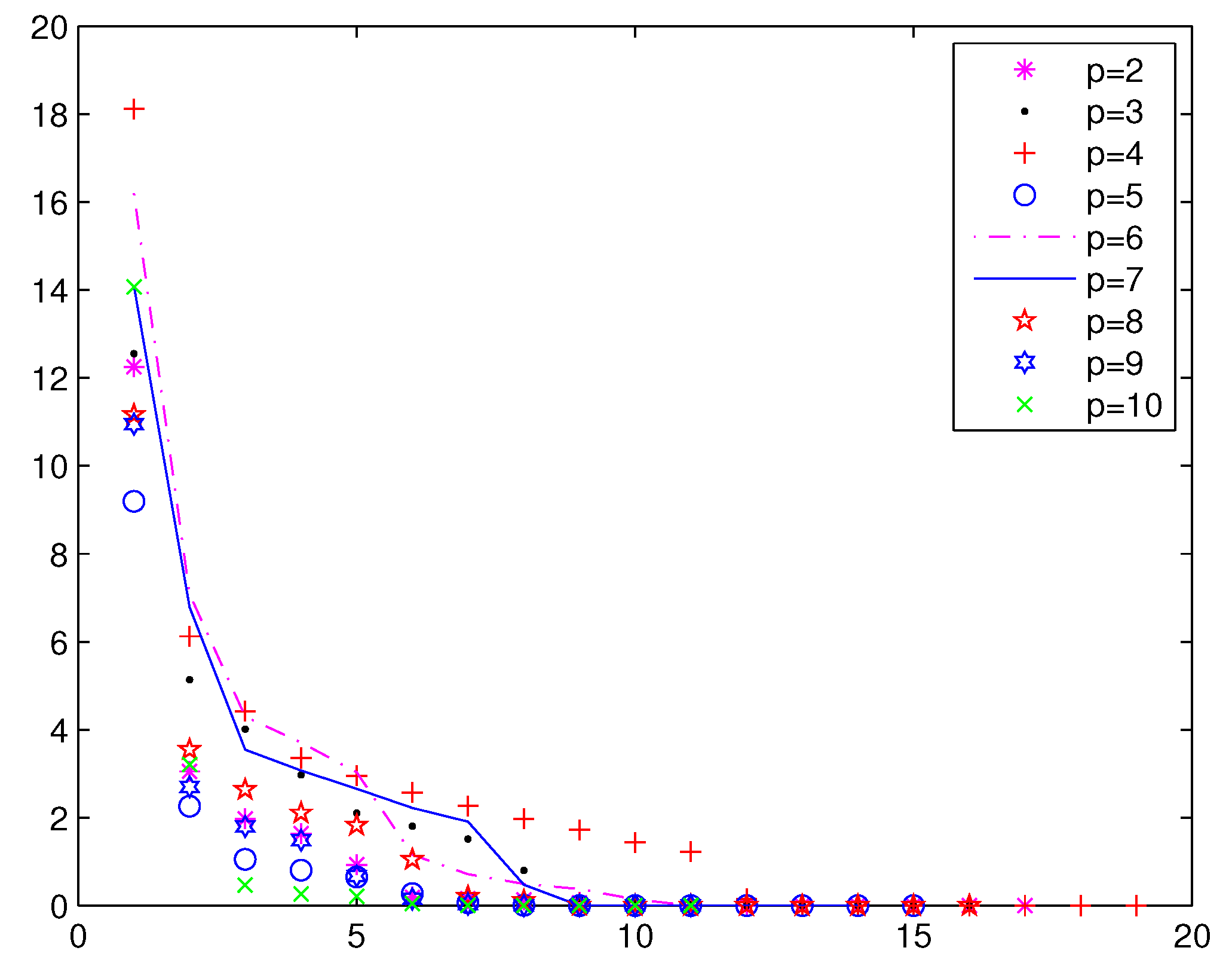
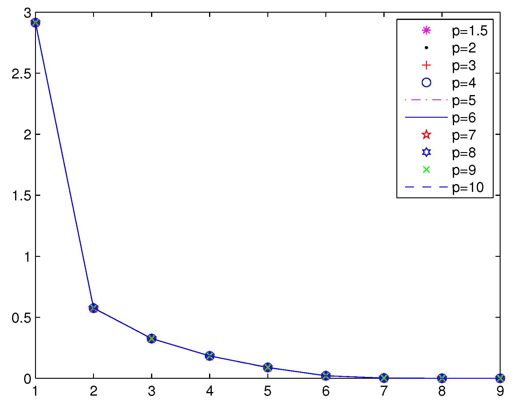
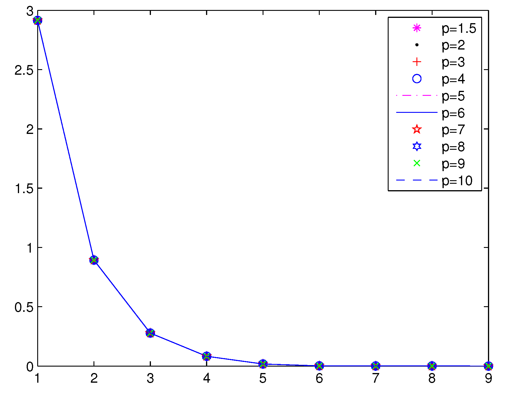
Example 2.

Consider $SLCP\left(M\right(\omega ),q(\omega \left)\right)$ with:

$$M\left(\omega \right)=\left(\begin{array}{ccc}1& -\omega & 0\\ -\omega & 2& \omega \\ 0& \omega & 3\end{array}\right),q\left(\omega \right)=\left(\begin{array}{c}3-2\omega \\ -2-\omega \\ -3-\omega \end{array}\right),$$

where $\Omega =\{{\omega }_1,{\omega }_2\}=\{0,1\},$ and $p_i=P({\omega }_i\in \Omega )=0.5,i=1,2$.

Numerical results are given in Table 3, Figure 2 and Figure 3; $x_0$ are chosen randomly in ${\Re }^3$; $y_0$ are chosen randomly in ${\Re }^6$; and $\lambda =0.00000001$.

Table 3. Numerical results for Example 2.

		Method 1		STRM
p	x*	Final Value	Iteration	Final Value	Iteration
2.0	(0, 1, 1)	5.6439 × 10−17	17	5.000 × 10−17	80
3.0	(0, 1, 1)	5.0000 × 10−17	16	5.000 × 10−17	80
4.0	(0, 1, 1)	5.0002 × 10−17	19	5.000 × 10−17	72
5.0	(0, 1, 1)	5.0000 × 10−17	15	5.000 × 10−17	234
6.0	(0, 1, 1)	5.0000 × 10−17	13	5.000 × 10−17	234
7.0	(0, 1, 1)	5.0000 × 10−17	14	5.000 × 10−17	234
8.0	(0, 1, 1)	5.0000 × 10−17	16	5.000 × 10−17	234
9.0	(0, 1, 1)	5.0000 × 10−17	11	5.000 × 10−17	234
10	(0, 1, 1)	5.0000 × 10−17	11	5.000 × 10−17	234

Figure 3. Numerical results for Example 2 by Method 1. The x-axis represents the iteration step; the y-axis represents $\theta (x,y)=\frac{1}{2}{\parallel F(x,y)\parallel }^2$.

From Table 3, Figure 3 and Figure 4, we can see that the iterations of Method 1 are less than the STRM method. In Method 1, when $p=5$, the function value falls faster. When p is larger, a greater number of iterations is needed in the STRM method.

Figure 4. Numerical results for Example 2 by the STRM method. The x-axis represents the iteration step; the y-axis represents $\theta (x,y)=\frac{1}{2}{\parallel F(x,y)\parallel }^2$.

In Table 4, we also give the comparison of Method 1 with fmincon. For the propose of comparison, we fixed $p=10$ and the same initial points.

Table 4. Numerical results for Example 2 by Method 1 and fmincon.

	x*	Final Value
Method 1	(0, 1, 1)	5.0000 × 10−17
fmincon	(0, 1, 1)	4.9780 × 10−14

From Table 4, we can see that Method 1 is also more effective than fmincon.

Example 3.

This example is a refinery production problem, which is also considered in [2,13].

The problem is defined as:

$$M\left(\omega \right)=\left(\begin{array}{ccccc}0& 0& 1& -2-{\omega }_1& -3\\ 0& 0& 1& -6& {\omega }_2-3.4\\ -1& -1& 0& 0& 0\\ 2+{\omega }_1& 6& 0& -{\omega }_3& -{\omega }_3\\ 3& 3.4-{\omega }_2& 0& -{\omega }_4& {\omega }_4\end{array}\right),$$

$$q\left(\omega \right)=\left(\begin{array}{c}c\\ -b\\ -180-{\omega }_3\\ -162-{\omega }_4\end{array}\right),$$

where ${\omega }_1$, ${\omega }_2$, ${\omega }_3$ and ${\omega }_4$ satisfy the following distribution:

$$distr{\omega }_1\approx u[-0.8,0.8],$$

$$distr{\omega }_2\approx exp(\lambda =2.5),$$

$$distr{\omega }_3\approx N(0,12),$$

$$distr{\omega }_4\approx N(0,9).$$

• Generate samples ${\omega }_j^k,j=1,2,3,4,k=1,2,\dots ,K,$ respectively, from their 99% confidence intervals (except uniform distributions):

  $${\omega }_1\in I_1=[-0.8,0.8],$$

  $${\omega }_2\in I_2=[0.0,1.84],$$

  $${\omega }_3\in I_3=[-30.91,30.91],$$

  $${\omega }_4\in I_4=[-23.18,23.18],$$
• For each $j,$ divide the $I_j$ into $m_j$ cells $I_{j,i}$, $i=1,2,\dots ,m_j$.
• For each $(j,i),$ calculate the average ${\upsilon }_{j,i}$ of ${\omega }_j^k$; it belongs to $I_{j,i}$.
• For each $(j,i),$ the estimated probability of ${\upsilon }_{j,i}$ is $p_{j,i}=k_{j,i}/K,$ where $k_{j,i}$ is the number of ${\omega }_j^k\in I_{j,i}$.
• Let $N=m_1\times m_2\times m_3\times m_4$, and set the joint distribution of $\{({\omega }^{\ell },p^{\ell }),\ell =1,2,\dots ,N\}$,

  $${\omega }^{\ell }=\left(\begin{array}{c}{\upsilon }_{1,i_1}\\ {\upsilon }_{2,i_2}\\ {\upsilon }_{3,i_3}\\ {\upsilon }_{4,i_4}\end{array}\right),p^{\ell }=p_{1,i_1}{p}_{2,i_2}{p}_{3,i_3}{p}_{4,i_4}$$

  for $i_1=1,\dots ,m_1$, $i_2=1,\dots ,m_2$, $i_3=1,\dots ,m_3$, $i_4=1,\dots ,m_4$.

In the following part of this section, we use Method 1 to solve the constrained optimization problem:

$$\underset{z\ge 0}{min}\theta \left(z\right)=\frac{1}{2}{\parallel F\left(z\right)\parallel }^2,$$

where $z=(x,y),$

$$F(x,y)=\left(\begin{array}{c}{\varphi }_n\left(x\right)\\ M\left({\omega }^{\ell }\right)x+q\left({\omega }^{\ell }\right)-y_{\ell },\ell =1\cdots N\end{array}\right).$$

and:

$${\varphi }_n\left(x\right)=\left(\begin{array}{c}\lambda {\varphi }_p(x_i,{\overline{M}}_{i}x+{\overline{q}}_i),i=1\cdots 5\\ ⋮\\ (1-\lambda ){\varphi }_{+}(x_i,{\overline{M}}_{i}x+{\overline{q}}_i),i=1\cdots 5\end{array}\right).$$

Now, we examine the following two conditions:

$$Condition1:{\omega }_1\equiv 0,{\omega }_2\equiv 0,m_3=15,m_4=15.$$

$$Condition2:m_1=5,m_2=9,m_3=7,m_4=11.$$

The numerical results of Example 3 are given in Table 5 and Table 6, where $\Psi \left(x\right)=\frac{1}{2}{\parallel {\varphi }_n\left(x\right)\parallel }^2$ is the merit function; $\theta (x,y)=\frac{1}{2}{\parallel F(x,y)\parallel }^2$; $k={10}^i,i=3,4,5$. $2x_1+3x_2$ is the initial production cost; and $\lambda =0.5$.

Table 5. Numerical results for Example 3 based on Condition 1.

p	k	xk	θ(zk)	Ψ(xk)	$2{\mathit{x}}_1^{\mathit{k}}+3{\mathit{x}}_2^{\mathit{k}}$
2	103	(42.6730, 15.8000, 0, 0.2848, 0.4688)	18.1932	5.1078	132.7462
2	104	(42.6057, 15.8216, 0, 0.2844, 0.4694)	5.2138	5.0089	132.6760
2	105	(42.0369, 16.0037, 0, 0.2791, 0.4740)	4.3894	4.2424	132.0850
4	103	(42.7120, 15.7720, 0, 0.2872, 0.4829)	1999.1	5.3083	132.7399
4	104	(42.6301, 15.7986, 0, 0.2844, 0.4694)	5.2164	5.0103	132.6559
4	105	(42.0487, 15.9888, 0, 0.2791, 0.4740)	4.3826	4.2359	132.0628
6	103	(42.7277, 15.7628, 0, 0.2853, 0.4687)	5.3534	5.1372	132.7438
6	104	(42.6539, 15.7870, 0, 0.2846, 0.4692)	5.2433	5.0360	132.6688
6	105	(42.0594, 15.9826, 0, 0.2791, 0.4740)	4.3925	4.2458	132.0667

Table 6. Numerical results for Example 3 based on Condition 2.

p	k	xk	θ(zk)	Ψ(xk)	$2{\mathit{x}}_1^{\mathit{k}}+3{\mathit{x}}_2^{\mathit{k}}$
2	103	(42.6799, 15.7988, 0, 0.2833, 0.4704)	5.3426	5.1369	132.7562
2	104	(42.5951, 15.8259, 0, 0.2826, 0.4706)	5.2120	5.0197	132.6679
2	105	(41.9961, 16.0177, 0, 0.2773, 0.4752)	4.3428	4.2083	132.0453
4	103	(42.7005, 15.7755, 0, 0.2846, 0.4717)	23.7543	5.1012	132.7276
4	104	(42.6135, 15.8036, 0, 0.2826, 0.4707)	5.2027	5.0096	132.6377
4	105	(41.9980, 16.0049, 0, 0.2772, 0.4753)	4.3207	4.1872	132.0108
6	103	(42.7599, 15.7531, 0, 0.2838, 0.4686)	55.2438	5.2217	132.7789
6	104	(42.6568, 15.7867, 0, 0.2829, 0.4703)	5.2612	5.0652	132.6738
6	105	(42.0153, 15.9977, 0, 0.2773, 0.4753)	4.3411	4.2060	132.0235

In [13], in the case of ${\omega }_1\equiv 0,{\omega }_2\equiv 0.4,m_3=15,m_4=15$. Kall and Wallace get the optimal solution $(x_1,x_2)=(38.539,20.539)$; initial production cost $2x_1+3x_2=138.695$. Here, by Method 1, we get the optimal solution $(x_1,x_2)=(41.6939,16.1036),$ and the production cost is $2x_1+3x_2=131.6985$.

Remark 1.

In this paper, we use:

$${\omega }_i=\left\{\begin{array}{c}{\omega }_j,i=j,\\ E\left({\omega }_j\right),i\ne j.\end{array}\right.$$

(14)

The computation cost of our method is greatly reduced. In fact, when we think about the general case of ${\omega }_1,{\omega }_2,{\omega }_3$ and ${\omega }_4$ varying the random distribution of discrete approximation by a 5-, 9-, 7- and 11-point distribution, respectively. This yields a joint discrete distribution of $5\times 9\times 7\times 11=3465$ realizations. Then, $F\left(z\right)$ is a function of 17,335 $(3465\times 5+10=$ 17,335) dimensions. This is a more complex optimization problem.

In the following part of this subsection, we give a large-scale stochastic linear complementarity problem named the stochastic Murty problem. When $\Omega =\left\{\omega \right|\omega =\frac{1}{2}\},$ the large-scale stochastic linear complementarity problem reduces to the Murty problem, which is intensively studied in [25,26,27,28,29].

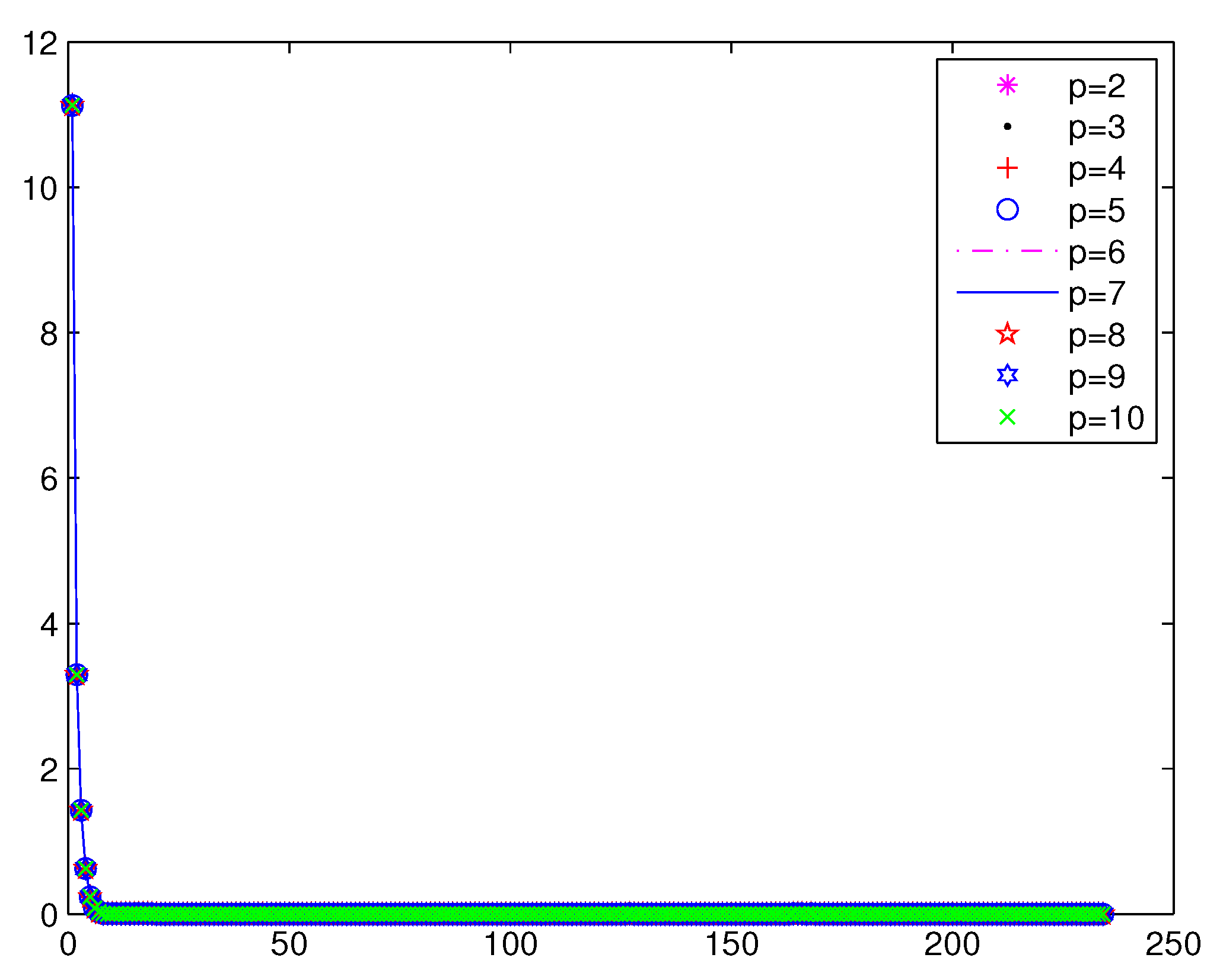
Example 4.

(Stochastic Murty problem) Consider $SLCP\left(M\right(\omega ),q(\omega \left)\right)$ with:

$$M\left(\omega \right)=\left(\begin{array}{cccc}\frac{1}{2}+\omega & 2& \cdots & 2\\ 0& \frac{1}{2}+\omega & \cdots & 2\\ ⋮& ⋮& \ddots & \\ 0& \cdots & & \frac{1}{2}+\omega \end{array}\right),q\left(\omega \right)=\left(\begin{array}{c}-\frac{3}{2}+\omega \\ -\frac{3}{2}+\omega \\ ⋮\\ -\frac{3}{2}+\omega \end{array}\right),$$

where $M\left(\omega \right)\in {\Re }^{n\times n}$, $q\left(\omega \right)\in {\Re }^n$. $\Omega =\{{\omega }_1,{\omega }_2\}=\{0,1\},$ and $p_i=P({\omega }_i\in \Omega )=0.5,i=1,2$.

In Table 7, we give the comparison of Method 1 with the SQP method in the fmincon tool box, when the dimensions of Example 4 are 10, 100, 200, 300 and 400; where $\theta (x,y)=\frac{1}{2}{\parallel F(x,y)\parallel }^2$. $x_0$ are chosen randomly in ${\Re }^n$. $y_0$ are chosen randomly in ${\Re }^{2n}$, $\lambda =0.0001$.

Table 7. Numerical results for Example 4.

DIM	p	Final Value of Method 1	Final Value of Fmincon
10	2	1.6000 × 10−3	0.4315
10	4	1.6000 × 10−3	0.4315
10	6	1.6000 × 10−3	0.4315
100	2	3.8000 × 10−3	0.4426
100	4	4.5000 × 10−3	0.4461
100	6	4.0000 × 10−3	0.4502
200	2	4.6000 × 10−3	0.5101
200	4	4.8000 × 10−3	0.4123
200	6	4.6000 × 10−3	0.5108
300	2	1.3263 × 10−4	0.5394
300	4	0.4373 × 10−3	0.5665
300	6	6.3331 × 10−4	0.5395
400	2	4.6550 × 10−4	0.4575
400	4	8.0495 × 10−4	0.5365
400	6	3.2255 × 10−4	0.5514

Remark 2.

By the numerical results of Example 4, we can see that Method 1 is very suitable to solve large-scale SLCP. Moreover, Method 1 can be used flexible by adjusting the value of p.

5. Conclusions

In this paper, we introduced a feasible nonsmooth Levenberg–Marquardt-type method to solve the stochastic linear complementarity problems with finitely many elements. This method used a linear least squares reformulation of the stochastic linear complementarity problem and applied a feasible nonsmooth Levenberg–Marquardt-type method to solve the reformulated problem. The finally given numerical results showed that the given method is efficient to solve the large-scale stochastic linear complementarity problem and related refinery production problem. Additionally, the method can choose the initial points in a large scope with less computations and high precision.