Comment on: On the Kung-Traub Conjecture for Iterative Methods for Solving Quadratic Equations. Algorithms 2016, 9, 1

Abstract

Kung-Traub conjecture states that an iterative method without memory for finding the simple zero of a scalar equation could achieve convergence order $2^{d-1}$, and d is the total number of function evaluations. In an article “Babajee, D.K.R. On the Kung-Traub Conjecture for Iterative Methods for Solving Quadratic Equations, Algorithms 2016, 9, 1, doi:10.3390/a9010001”, the author has shown that Kung-Traub conjecture is not valid for the quadratic equation and proposed an iterative method for the scalar and vector quadratic equations. In this comment, we have shown that we first reported the aforementioned iterative method.

1. Iterative Methods for Solving Quadratic Equations Presented in [1]

According to Kung-Traub conjecture (KTC) [2], an iterative method without memory for solving nonlinear equations in the case of simple zeros, could achieve a maximum convergence order of $2^{d-1}$, where d is the number of function evaluations. Recently, an article was published for solving quadratic equations [1] with arbitrary order of convergence by using one function and two derivatives evaluations. The details of the proposed formulation in [1] is given as follows. Let $f\left(x\right)={\kappa }_2{x}^2+{\kappa }_{1}x+{\kappa }_0$ be a quadratic function where ${\kappa }_2\ne 0$ and ${\kappa }_1$, ${\kappa }_0$ are constants. The proposed iteration function ${\psi }_{{(r+2)}^{\text{th}}\text{BQIM}}\left(x\right)$ in [1] is

$$\begin{array}{c}\hfill \left\{\begin{array}{cc}& u\left(x\right)=\frac{f\left(x\right)}{f^{\prime }\left(x\right)}\hfill \\ & \tau =\frac{f^{\prime }\left(x-2/3u\left(x\right)\right)}{f^{\prime }\left(x\right)}\hfill \\ & H(\tau ,r)=1+{\displaystyle \sum _{i=1}^r}{a}_i{(\tau -1)}^i\hfill \\ & {\psi }_{{(r+2)}^{\text{th}}\text{BQIM}}\left(x\right)=x-u\left(x\right)H(\tau ,r)\hfill \end{array}\right.\end{array}$$

(1)

The error equation of Equation (1) is given as ${\psi }_{{(r+2)}^{\text{th}}\text{BQIM}}\left(x\right)-x^{*}=C_r\left(c_2^{r+1}\right){\left(e^{\left(k\right)}\right)}^{r+2}+O\left({\left(e^{\left(k\right)}\right)}^{r+3}\right)$ where $C_r$ is asymptotic error constant, $x^{*}$ is the simple root of quadratic equation and $c_2=1/2f^{\prime }{\left(x^{*}\right)}^{-1}{f}^{″}\left(x^{*}\right)$. The error equation clearly shows that KTC is not valid in the case of quadratic equations. By using binomial expansion, the weight function $H(\tau ,r)$ can be written as

$$\begin{array}{c}\hfill \begin{array}{cc}& H(\tau ,r)=1+{\displaystyle \sum _{i=1}^r}{\displaystyle \sum _{j=0}^i}{a}_i\left(\begin{array}{c}i\\ i-j\end{array}\right){(-1)}^{(i-j)}{\tau }^j\hfill \\ & H(\tau ,r)=1+{\displaystyle \sum _{i=0}^r}{b}_i{\tau }^i\hfill \end{array}\end{array}$$

(2)

where $b_i$ is constant and can be computed by comparing two expressions of $H(\tau ,r)$ in Equation (2). The powers of τ can be computed recursively and hence the iteration function Equation (1) is written as

$$\begin{array}{c}\hfill \left\{\begin{array}{cc}& u\left(x\right)=\frac{f\left(x\right)}{f^{\prime }\left(x\right)}\hfill \\ & y=x-2/3u\left(x\right)\hfill \\ & \tau =\frac{f^{\prime }\left(y\right)}{f^{\prime }\left(x\right)}\hfill \\ & {\varphi }_0=u\left(x\right)\hfill \\ & \text{for}i=1,r\hfill \\ & {\varphi }_i=\tau {\varphi }_{i-1}\hfill \\ & \text{end}\hfill \\ & {\psi }_{{(r+2)}^{\text{th}}\text{BQIM}}\left(x\right)=x-{\varphi }_0-{\displaystyle \sum _{i=0}^r}{b}_i{\varphi }_i.\hfill \end{array}\right.\end{array}$$

(3)

The computationally efficient vector version of iteration function Equation (3) is

$$\begin{array}{c}\hfill \left\{\begin{array}{cc}& {\mathbf{F}}^{\prime }\left(\mathbf{x}\right){\mathbf{\varphi }}_0=\mathbf{F}\left(\mathbf{x}\right)\hfill \\ & \mathbf{y}=\mathbf{x}-2/3{\mathbf{\varphi }}_0\hfill \\ & \text{for}i=1,r\hfill \\ & {\mathbf{F}}^{\prime }\left(\mathbf{x}\right){\mathbf{\varphi }}_i={\mathbf{F}}^{\prime }\left(\mathbf{y}\right){\mathbf{\varphi }}_{i-1}\hfill \\ & \text{end}\hfill \\ & {\mathbf{\psi }}_{{(r+2)}^{\text{th}}\text{BQIM}}\left(\mathbf{x}\right)=\mathbf{x}-{\mathbf{\varphi }}_0-{\displaystyle \sum _{i=0}^r}{b}_i{\mathbf{\varphi }}_i.\hfill \end{array}\right.\end{array}$$

(4)

2. Iterative Methods for Solving Matrix-Vector Quadratic Equations Presented in [3]

In this direction, a manuscript [3] was posted on 4 May 2015 on Researchgate in which the author provided models of three iterative methods, with their respective convergence orders, for computing the solution of matrix-vector quadratic equations. As the proposed iterative methods are valid for solving systems of nonlinear equations with quadratic nonlinearity, they are also valid for scalar quadratic equations. In the article [3] the model of iterative Method II can be written as:

$$\begin{array}{c}\hfill \left\{\begin{array}{c}{\mathbf{x}}_0=\text{initial}\text{guess}\hfill \\ {\mathbf{F}}^{\prime }\left({\mathbf{x}}_0\right){\mathbf{\varphi }}_1=\mathbf{F}\left({\mathbf{x}}_0\right)\hfill \\ {\mathbf{x}}_1={\mathbf{x}}_0+{\alpha }_{1,1}{\mathbf{\varphi }}_1\hfill \\ \text{for}i=1,m\hfill \\ {\mathbf{F}}^{\prime }\left({\mathbf{x}}_0\right){\mathbf{\varphi }}_{i+1}={\mathbf{F}}^{\prime }\left({\mathbf{x}}_1\right){\mathbf{\varphi }}_i\hfill \\ \text{end}\hfill \\ {\mathbf{x}}_2={\mathbf{x}}_0+{\displaystyle \sum _{j=1}^m}{\alpha }_{2,j}{\mathbf{\varphi }}_j\hfill \\ {\mathbf{x}}_2={\mathbf{x}}_0\hfill \end{array}\right.\end{array}$$

(5)

where $\mathbf{F}\left(\mathbf{x}\right)=\mathbf{0}$ is a quadratic equation i.e., ${\mathbf{F}}^{″}\left(\mathbf{x}\right)=\mathbf{B}$ is a bilinear form and ${\mathbf{F}}^{\left(s\right)}\left(\mathbf{x}\right)=\mathbf{O}$ (zero tensor) for $s\ge 3$ and the convergence order is $m+2$. The scalar version of iterative method Equation (5) can be written as

$$\begin{array}{c}\hfill \left\{\begin{array}{c}{x}_0=\text{initial}\text{guess}\hfill \\ f^{\prime }\left(x_0\right){\varphi }_1=f\left(x_0\right)\hfill \\ x_1=x_0+{\alpha }_{1,1}{\varphi }_1\hfill \\ \text{for}i=1,m\hfill \\ f^{\prime }\left(x_0\right){\varphi }_{i+1}=f^{\prime }\left(x_1\right){\varphi }_i\hfill \\ \text{end}\hfill \\ x_2=x_0+{\displaystyle \sum _{j=1}^m}{\alpha }_{2,j}{\varphi }_j\hfill \\ x_0=x_2\hfill \end{array}\right.\end{array}$$

(6)

where $f\left(x\right)=a{x}^2+bx+c$ with $a\ne 0$ and convergence order is $m+2$. The convergence proofs of different iterative methods are established in Figure 1, Figure 2, Figure 3 and Figure 4. We can see that the error equations in all cases are the same. The Figure 4 shows that the iterative method (1) is a particular case of iterative method Equation (6) for ${\alpha }_{1,1}=-2/3$. Finally we provide the convergence proof of the iterative method Equation (5).

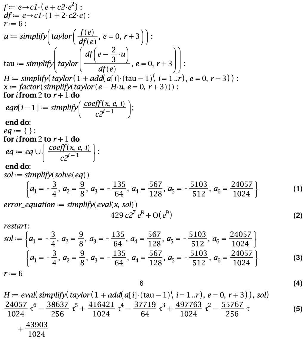
Figure 1. Iterative method Equation (1).

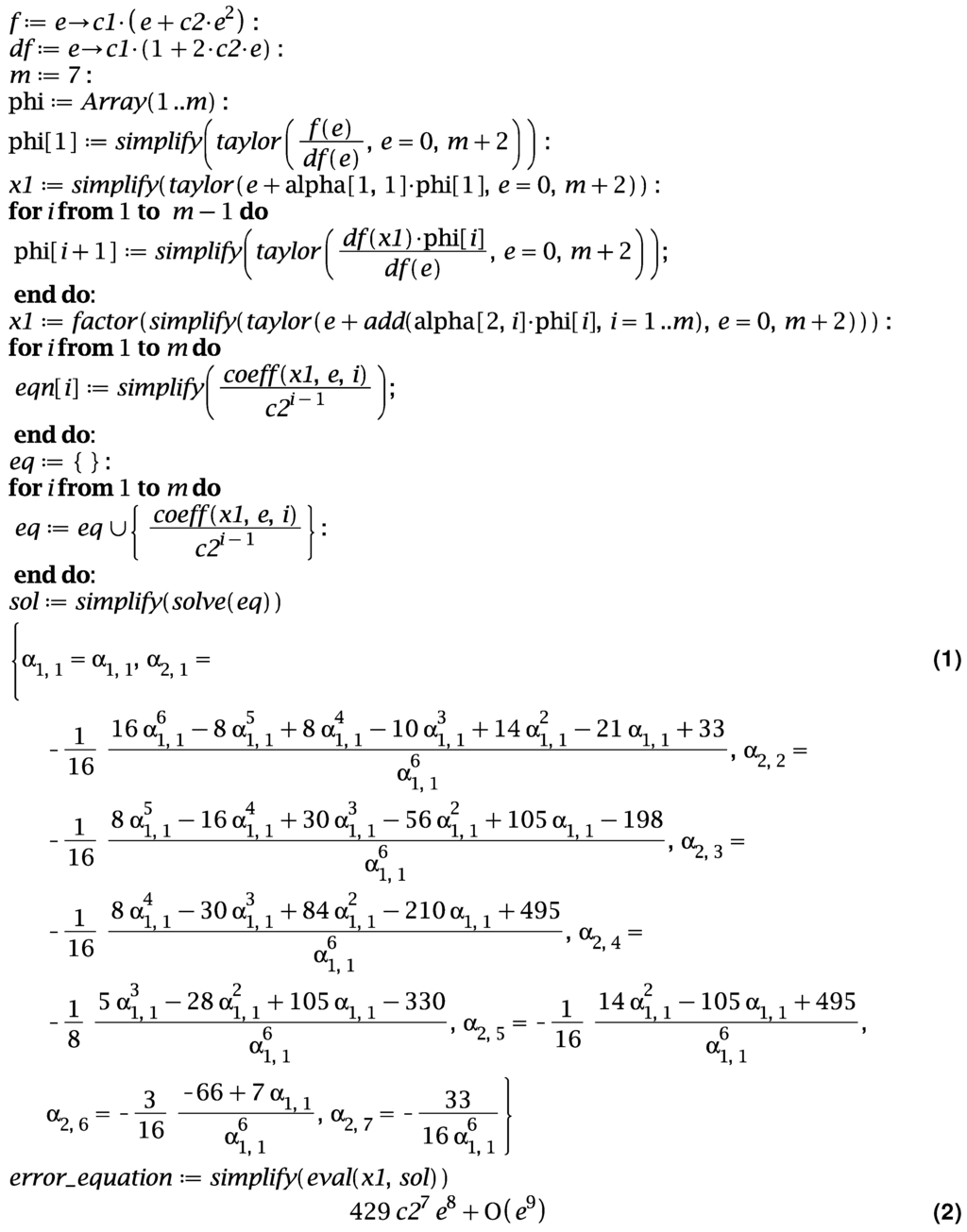
Figure 2. Iterative method Equation (6) for arbitrary finite ${\alpha }_{1,1}$.

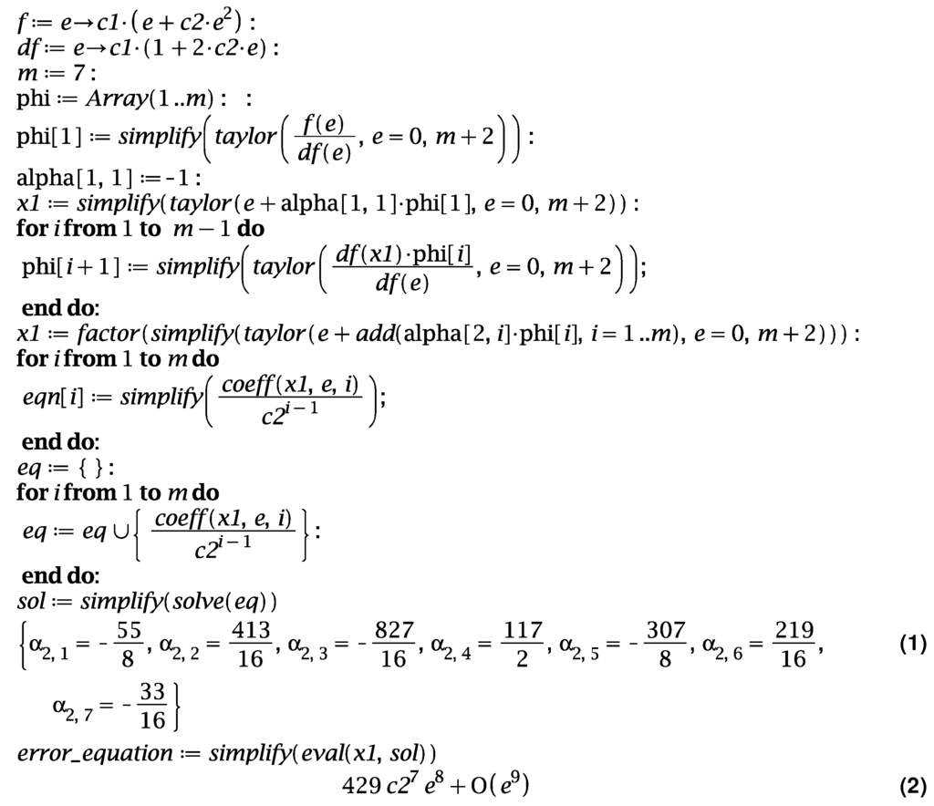
Figure 3. Iterative method (6) for ${\alpha }_{1,1}=-1$.

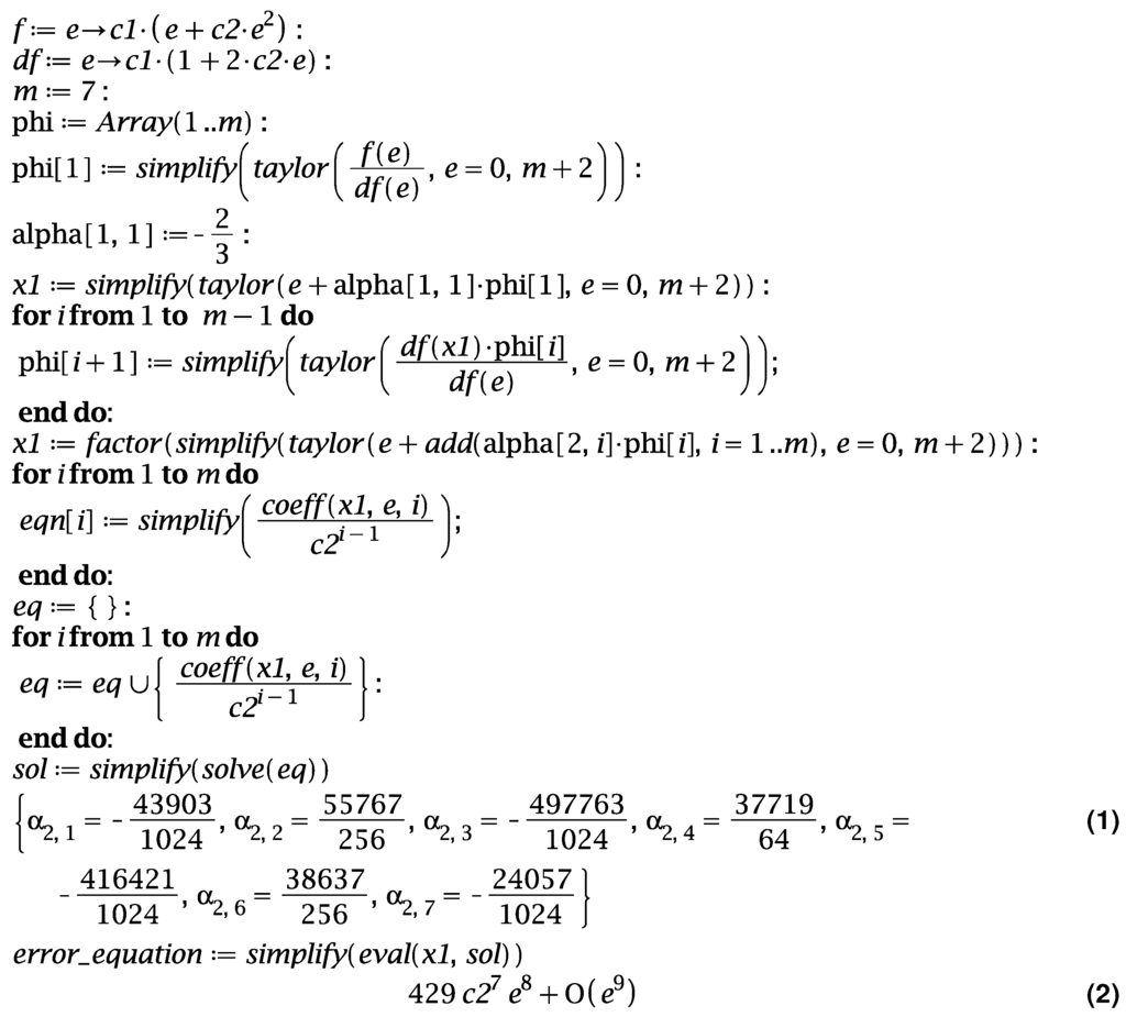
Figure 4. Iterative method (6) for ${\alpha }_{1,1}=-2/3$.

Theorem 2.1. 

Let $\mathbf{F}:\mathbf{D}\subseteq {\mathbb{R}}^n⟶{\mathbb{R}}^n$ be a function with all continuous Fréchet derivatives, ${\mathbf{F}}^{″}\left(\mathbf{x}\right)=\mathbf{B}$ and ${\mathbf{F}}^{\left(j\right)}\left(\mathbf{x}\right)=\mathbf{O}$ for $j\ge 3$, where $\mathbf{B}$ is a bilinear form and $\mathbf{D}$ is convex open subset of ${\mathbb{R}}^n$. If we take ${\mathbf{x}}_0$ in the vicinity of a simple root ${\mathbf{x}}^{*}$ of $\mathbf{F}\left(\mathbf{x}\right)=\mathbf{0}$ then the sequence of successive approximation generated by iterative method Equation (5) for $m=6$ and ${\alpha }_{1,1}=-2/3$ converges to ${\mathbf{x}}^{*}$ with convergence order eight.

Proof. 

We denote ${\mathbf{e}}_k={\mathbf{x}}_k-{\mathbf{x}}^{*}$, ${\mathbf{C}}_1={\mathbf{F}}^{\prime }\left({\mathbf{x}}^{*}\right)$ and ${\mathbf{C}}_2={\mathbf{F}}^{\prime }{\left({\mathbf{x}}^{*}\right)}^{-1}{\mathbf{F}}^{″}\left({\mathbf{x}}^{*}\right)/2$. By expanding ${\mathbf{F}}^{\prime }\left({\mathbf{x}}_0\right)$ around ${\mathbf{x}}^{*}$ we get

$$\begin{array}{c}\hfill \mathbf{F}\left({\mathbf{x}}_0\right)={\mathbf{C}}_1\left({\mathbf{e}}_0+{\mathbf{C}}_2{\mathbf{e}}_0^2\right)\end{array}$$

(7)

The Fréchet derivative of Equation (7) with respective to ${\mathbf{e}}_0$ is

$$\begin{array}{c}\hfill {\mathbf{F}}^{\prime }\left({\mathbf{x}}_0\right)={\mathbf{C}}_1\left(\mathbf{I}+2{\mathbf{C}}_2{\mathbf{e}}_0\right)\end{array}$$

(8)

The inverse of Equation (8) is

$$\begin{array}{c}\hfill \begin{array}{cc}\hfill {\mathbf{F}}^{\prime }{\left({\mathbf{x}}_0\right)}^{-1}=& (I-2{\mathbf{C}}_2{\mathbf{e}}_0+4{\mathbf{C}}_2^2{\mathbf{e}}_0^2-8{\mathbf{C}}_2^3{\mathbf{e}}_0^3+16{\mathbf{C}}_2^4{\mathbf{e}}_0^4-32{\mathbf{C}}_2^5{\mathbf{e}}_0^5+64{\mathbf{C}}_2^6{\mathbf{e}}_0^6-128{\mathbf{C}}_2^7{\mathbf{e}}_0^7\hfill \\ & +256{\mathbf{C}}_2^8{\mathbf{e}}_0^8){\mathbf{C}}_1^{-1}+O\left({\mathbf{e}}_0^9\right)\hfill \end{array}\end{array}$$

(9)

We compute ${\mathbf{\varphi }}_1$ using Equations (9) and (7)

$$\begin{array}{c}\hfill {\mathbf{\varphi }}_1={\mathbf{e}}_0-{\mathbf{C}}_2{\mathbf{e}}_0^2+2{\mathbf{C}}_2^2{\mathbf{e}}_0^3-4{\mathbf{C}}_2^3{\mathbf{e}}_0^4+8{\mathbf{C}}_2^4{\mathbf{e}}_0^5-16{\mathbf{C}}_2^5{\mathbf{e}}_0^6+32{\mathbf{C}}_2^6{\mathbf{e}}_0^7-64{\mathbf{C}}_2^7{\mathbf{e}}_0^8+O\left({\mathbf{e}}_0^9\right).\end{array}$$

(10)

The expression for ${\mathbf{e}}_1$ is

$$\begin{array}{c}\hfill \begin{array}{cc}\hfill {\mathbf{e}}_1=& 1/3\left({\mathbf{e}}_0+2{\mathbf{C}}_2{\mathbf{e}}_0^2-4{\mathbf{C}}_2^2{\mathbf{e}}_0^3+8{\mathbf{C}}_2^3{\mathbf{e}}_0^4-16{\mathbf{C}}_2^4{\mathbf{e}}_0^5+32{\mathbf{C}}_2^5{\mathbf{e}}_0^6+64{\mathbf{C}}_2^6{\mathbf{e}}_0^7+128{\mathbf{C}}_2^7{\mathbf{e}}_0^8\right)\hfill \\ & +O\left({\mathbf{e}}_0^9\right)\hfill \end{array}\end{array}$$

(11)

First order Fréchet derivative of $\mathbf{F}\left(\mathbf{x}\right)$ at ${\mathbf{x}}_1$ is

$$\begin{array}{c}\hfill \begin{array}{cc}\hfill {\mathbf{F}}^{\prime }\left({\mathbf{x}}_1\right)=& {\mathbf{C}}_1(\mathbf{I}+1/3(2{\mathbf{C}}_2{\mathbf{e}}_0+4{\mathbf{C}}_2^2{\mathbf{e}}_0^2-8{\mathbf{C}}_2^3{\mathbf{e}}_0^3+16{\mathbf{C}}_2^4{\mathbf{e}}_0^4-32{\mathbf{C}}_2^5{\mathbf{e}}_0^5+64{\mathbf{C}}_2^6{\mathbf{e}}_0^6\hfill \\ & -128{\mathbf{C}}_2^7{\mathbf{e}}_0^7+256{\mathbf{C}}_2^8{\mathbf{e}}_0^8\left)\right)+O\left({\mathbf{e}}_0^9\right)\hfill \end{array}\end{array}$$

(12)

Next we compute $\mathbf{M}={\mathbf{F}}^{\prime }{\left({\mathbf{x}}_0\right)}^{-1}{\mathbf{F}}^{\prime }\left({\mathbf{x}}_1\right)$

$$\begin{array}{c}\hfill \begin{array}{cc}\hfill \mathbf{M}=& \mathbf{I}-4/3{\mathbf{C}}_2{\mathbf{e}}_0+4{\mathbf{C}}_2^2{\mathbf{e}}_0^2-32/3{\mathbf{C}}_2^3{\mathbf{e}}_0^3+80/3{\mathbf{C}}_2^4{\mathbf{e}}_0^4-64{\mathbf{C}}_2^5{\mathbf{e}}_0^5+448/3{\mathbf{C}}_2^6{\mathbf{e}}_0^6\hfill \\ & -1024/3{\mathbf{C}}_2^7{\mathbf{e}}_0^7+768{\mathbf{C}}_2^8{\mathbf{e}}_0^8+O\left({\mathbf{e}}_0^9\right)\hfill \end{array}\end{array}$$

(13)

with help of Equation (13), we obtain the expressions for ${\mathbf{\varphi }}_i$ for $i\in \{2,3,4,5,6,7\}$

$$\begin{array}{c}\hfill \begin{array}{cc}\hfill {\mathbf{\varphi }}_2=& {\mathbf{e}}_0-7/3{\mathbf{C}}_2{\mathbf{e}}_0^2+22/3{\mathbf{C}}_2^2{\mathbf{e}}_0^3-64/3{\mathbf{C}}_2^3{\mathbf{e}}_0^4+176/3{\mathbf{C}}_2^4{\mathbf{e}}_0^5-464/3{\mathbf{C}}_2^5{\mathbf{e}}_0^6+1184/3{\mathbf{C}}_2^6{\mathbf{e}}_0^7\hfill \\ & -2944/3{\mathbf{C}}_2^7{\mathbf{e}}_0^8+O\left({\mathbf{e}}_0^9\right)\hfill \\ \hfill {\mathbf{\varphi }}_3=& {\mathbf{e}}_0-11/3{\mathbf{C}}_2{\mathbf{e}}_0^2+130/9{\mathbf{C}}_2^2{\mathbf{e}}_0^3-460/9{\mathbf{C}}_2^3{\mathbf{e}}_0^4+168{\mathbf{C}}_2^4{\mathbf{e}}_0^5-1568/3{\mathbf{C}}_2^5{\mathbf{e}}_0^6\hfill \\ & +4672/3{\mathbf{C}}_2^6{\mathbf{e}}_0^7-4480{\mathbf{C}}_2^7{\mathbf{e}}_0^8+O\left({\mathbf{e}}_0^9\right)\hfill \\ \hfill {\mathbf{\varphi }}_4=& {\mathbf{e}}_0-5{\mathbf{C}}_2{\mathbf{e}}_0^2+70/3{\mathbf{C}}_2^2{\mathbf{e}}_0^3-2584/27{\mathbf{C}}_2^3{\mathbf{e}}_0^4+9712/27{\mathbf{C}}_2^4{\mathbf{e}}_0^5-34208/27{\mathbf{C}}_2^5{\mathbf{e}}_0^6\hfill \\ & +114496/27{\mathbf{C}}_2^6{\mathbf{e}}_0^7-367616/27{\mathbf{C}}_2^7{\mathbf{e}}_0^8+O\left({\mathbf{e}}_0^9\right)\hfill \\ \hfill {\mathbf{\varphi }}_5=& {\mathbf{e}}_0-19/3{\mathbf{C}}_2{\mathbf{e}}_0^2+34{\mathbf{C}}_2^2{\mathbf{e}}_0^3-4252/27{\mathbf{C}}_2^3{\mathbf{e}}_0^4+53512/81{\mathbf{C}}_2^4{\mathbf{e}}_0^5-208624/81{\mathbf{C}}_2^5{\mathbf{e}}_0^6\hfill \\ & +767968/81{\mathbf{C}}_2^6{\mathbf{e}}_0^7-2697920/81{\mathbf{C}}_2^7{\mathbf{e}}_0^8+O\left({\mathbf{e}}_0^9\right)\hfill \\ \hfill {\mathbf{\varphi }}_6=& {\mathbf{e}}_0-23/3{\mathbf{C}}_2{\mathbf{e}}_0^2+418/9{\mathbf{C}}_2^2{\mathbf{e}}_0^3-6448/27{\mathbf{C}}_2^3{\mathbf{e}}_0^4+89168/81{\mathbf{C}}_2^4{\mathbf{e}}_0^5\hfill \\ & -1137712/243{\mathbf{C}}_2^5{\mathbf{e}}_0^6+4543840/243{\mathbf{C}}_2^6{\mathbf{e}}_0^7-5747840/81{\mathbf{C}}_2^7{\mathbf{e}}_0^8+O\left({\mathbf{e}}_0^9\right)\hfill \\ \hfill {\mathbf{\varphi }}_7=& {\mathbf{e}}_0-9{\mathbf{C}}_2{\mathbf{e}}_0^2+182/3{\mathbf{C}}_2^2{\mathbf{e}}_0^3-9236/27{\mathbf{C}}_2^3{\mathbf{e}}_0^4+46264/27{\mathbf{C}}_2^4{\mathbf{e}}_0^5-637376/81{\mathbf{C}}_2^5{\mathbf{e}}_0^6\hfill \\ & +24618880/729{\mathbf{C}}_2^6{\mathbf{e}}_0^7-100011520/729{\mathbf{C}}_2^7{\mathbf{e}}_0^8+O\left({\mathbf{e}}_0^9\right).\hfill \end{array}\end{array}$$

(14)

We obtain expression for ${\mathbf{e}}_2$ by using Equation (14)

$$\begin{array}{cc}\hfill {\mathbf{e}}_2=& \left(1+{\alpha }_{2,1}+{\alpha }_{2,2}+{\alpha }_{2,3}+{\alpha }_{2,4}+{\alpha }_{2,5}+{\alpha }_{2,6}+{\alpha }_{2,7}\right){\mathbf{e}}_0\hfill \\ & +\left(-{\alpha }_{2,1}-7/3{\alpha }_{2,2}-11/3{\alpha }_{2,3}-5{\alpha }_{2,4}-19/3{\alpha }_{2,5}-23/3{\alpha }_{2,6}-9{\alpha }_{2,7}\right){\mathbf{C}}_2{\mathbf{e}}_0^2\hfill \\ & +(2{\alpha }_{2,1}+22/3{\alpha }_{2,2}+130/9{\alpha }_{2,3}+70/3{\alpha }_{2,4}+34{\alpha }_{2,5}{\mathbf{C}}_2^2+418/9{\alpha }_{2,6}\hfill \\ & +182/3{\alpha }_{2,7}){\mathbf{C}}_2^2{\mathbf{e}}_0^3+(-4{\alpha }_{2,1}-64/3{\alpha }_{2,2}-460/9{\alpha }_{2,3}-2584/27{\alpha }_{2,4}-4252/27{\alpha }_{2,5}\hfill \\ & -6448/27{\alpha }_{2,6}-9236/27{\alpha }_{2,7}){\mathbf{C}}_2^3{\mathbf{e}}_0^4+(8{\alpha }_{2,1}+176/3{\alpha }_{2,2}+168{\alpha }_{2,3}+9712/27{\alpha }_{2,4}\hfill \\ & +53512/81{\alpha }_{2,5}+89168/81{\alpha }_{2,6}+46264/27{\alpha }_{2,7}){\mathbf{C}}_2^4{\mathbf{e}}_0^5+(-16{\alpha }_{2,1}-464/3{\alpha }_{2,2}\hfill \\ & -1568/3{\alpha }_{2,3}-34208/27{\alpha }_{2,4}-208624/81{\alpha }_{2,5}-1137712/243{\alpha }_{2,6}\hfill \\ & -637376/81{\alpha }_{2,7}){\mathbf{C}}_2^5{\mathbf{e}}_0^6+(32{\alpha }_{2,1}+1184/3{\alpha }_{2,2}+4672/3{\alpha }_{2,3}+114496/27{\alpha }_{2,4}\hfill \\ & +767968/81{\alpha }_{2,5}+4543840/243{\alpha }_{2,6}+24618880/729{\alpha }_{2,7}){\mathbf{C}}_2^6{\mathbf{e}}_0^7+(-64{\alpha }_{2,1}\hfill \\ & -2944/3{\alpha }_{2,2}-4480{\alpha }_{2,3}-367616/27{\alpha }_{2,4}-2697920/81{\alpha }_{2,5}-5747840/81{\alpha }_{2,6}\hfill \\ & -100011520/729{\alpha }_{2,7}){\mathbf{C}}_2^7{\mathbf{e}}_0^8+O\left({\mathbf{e}}_0^9\right).\hfill \end{array}$$

(15)

By equating the coefficients of powers of ${\mathbf{e}}_0$ in Equation (15), we get system of seven equations

$$\begin{array}{c}\hfill \begin{array}{cc}\hfill e{q}_1:=& 1+{\alpha }_{2,1}+{\alpha }_{2,2}+{\alpha }_{2,3}+{\alpha }_{2,4}+{\alpha }_{2,5}+{\alpha }_{2,6}+{\alpha }_{2,7}=0\hfill \\ \hfill e{q}_2:=& -{\alpha }_{2,1}-7/3{\alpha }_{2,2}-11/3{\alpha }_{2,3}-5{\alpha }_{2,4}-19/3{\alpha }_{2,5}-23/3{\alpha }_{2,6}-9{\alpha }_{2,7}=0\hfill \\ \hfill e{q}_3:=& 2{\alpha }_{2,1}+22/3{\alpha }_{2,2}+130/9{\alpha }_{2,3}+70/3{\alpha }_{2,4}+34{\alpha }_{2,5}+418/9{\alpha }_{2,6}+182/3{\alpha }_{2,7}=0\hfill \\ \hfill e{q}_4:=& -4{\alpha }_{2,1}-64/3{\alpha }_{2,2}-460/9{\alpha }_{2,3}-2584/27{\alpha }_{2,4}-4252/27{\alpha }_{2,5}-6448/27{\alpha }_{2,6}\hfill \\ & -9236/27{\alpha }_{2,7}=0\hfill \\ \hfill e{q}_5:=& 8{\alpha }_{2,1}+176/3{\alpha }_{2,2}+168{\alpha }_{2,3}+9712/27{\alpha }_{2,4}+53512/81{\alpha }_{2,5}+89168/81{\alpha }_{2,6}\hfill \\ & +46264/27{\alpha }_{2,7}=0\hfill \\ \hfill e{q}_6:=& -16{\alpha }_{2,1}-464/3{\alpha }_{2,2}-1568/3{\alpha }_{2,3}-34208/27{\alpha }_{2,4}-208624/81{\alpha }_{2,5}\hfill \\ & -1137712/243{\alpha }_{2,6}-637376/81{\alpha }_{2,7}=0\hfill \\ \hfill e{q}_7:=& 32{\alpha }_{2,1}+1184/3{\alpha }_{2,2}+4672/3{\alpha }_{2,3}+114496/27{\alpha }_{2,4}+767968/81{\alpha }_{2,5}\hfill \\ & +4543840/243{\alpha }_{2,6}+24618880/729{\alpha }_{2,7}=0.\hfill \end{array}\end{array}$$

(16)

The solution set of seven equations is

$$\begin{array}{c}\hfill \begin{array}{cc}\hfill sol=& \{{\alpha }_{2,1}=-\frac{43903}{1024},{\alpha }_{2,2}=\frac{55767}{256},{\alpha }_{2,3}=-\frac{497763}{1024},{\alpha }_{2,4}=\frac{37719}{64},{\alpha }_{2,5}=-\frac{416421}{1024},\hfill \\ & {\alpha }_{2,6}=\frac{38637}{256},{\alpha }_{2,7}=-\frac{24057}{1024}\}.\hfill \end{array}\end{array}$$

(17)

After simplification the error equation we get

$$\begin{array}{c}\hfill {\mathbf{e}}_2=429{\mathbf{C}}_2^7{\mathbf{e}}_0^8+O\left({\mathbf{e}}_0^9\right).\end{array}$$

(18)

☐

As we have seen, the convergence order of the iterative method Equation (5) is eight for $m=6$ and this confirms our claimed order of convergence which is $s+2$ for $m=s$. Now we provide the proof of convergence order via mathematical induction.

Theorem 2.2. 

Let $\mathbf{F}:\mathbf{D}\subseteq {\mathbb{R}}^n⟶{\mathbb{R}}^n$ be a function with all continuous Fréchet derivatives, ${\mathbf{F}}^{″}\left(\mathbf{x}\right)=\mathbf{B}$ and ${\mathbf{F}}^{\left(j\right)}\left(\mathbf{x}\right)=\mathbf{O}$ for $j\ge 3$, where $\mathbf{B}$ is a bilinear form and $\mathbf{D}$ is a convex open subset of ${\mathbb{R}}^n$. If we take ${\mathbf{x}}_0$ in the vicinity of a simple root ${\mathbf{x}}^{*}$ of $\mathbf{F}\left(\mathbf{x}\right)=\mathbf{0}$ then the sequence of successive approximation generated by the iterative method Equation (5) for $m=s$ and ${\alpha }_{1,1}=-2/3$ converges to ${\mathbf{x}}^{*}$ with convergence order $s+2$.

Proof. 

We suppose that our claim about the convergence order of the iterative method Equation (5) is true for $m=s$, which means we have

$$\begin{array}{c}\hfill {\mathbf{e}}_2^{\left(s\right)}=H_s{\mathbf{C}}_2^{s-1}{\mathbf{e}}_0^{s+2}+O\left({\mathbf{e}}_0^{s+3}\right)\end{array}$$

(19)

where $H_s$ is asymptotic error constant and superscript “$\left(s\right)$” means the value of ${\mathbf{e}}_2$ when $m=s$. We can write ${\mathbf{e}}_2^{\left(s\right)}$

$$\begin{array}{c}\hfill {\mathbf{e}}_2^{\left(s\right)}={\mathbf{e}}_0-2/3{\mathbf{\varphi }}_1+\left({\alpha }_{2,1}+{\alpha }_{2,2}\mathbf{M}+\cdots +{\alpha }_{2,s-1}{\mathbf{M}}^s\right){\mathbf{\varphi }}_1+H_s{\mathbf{C}}_2^{s-1}{\mathbf{e}}_0^{s+2}+O\left({\mathbf{e}}_0^{s+3}\right)\end{array}$$

(20)

It is convenient to express the combination

$${\alpha }_{2,1}+{\alpha }_{2,2}\mathbf{M}+{\alpha }_{2,3}{\mathbf{M}}^2+\cdots +{\alpha }_{2,s+1}{\mathbf{M}}^s$$

in the powers of $\mathbf{I}-\mathbf{M}$ [1], we establish the following identity

$$\begin{array}{c}\hfill {\alpha }_{2,1}+{\alpha }_{2,2}\mathbf{M}+\cdots +{\alpha }_{2,s-1}{\mathbf{M}}^s\equiv {\beta }_{2,1}+{\beta }_{2,2}\left(\mathbf{I}-\mathbf{M}\right)+\cdots +{\beta }_{2,s-1}{\left(\mathbf{I}-\mathbf{M}\right)}^s\end{array}$$

(21)

By comparing the same powers of $\mathbf{M}$ on both sides we can easily compute the value of ${\beta }_i$’s. By using Equation (21), error Equation (20) can be written as

$$\begin{array}{c}\hfill \begin{array}{cc}\hfill {\mathbf{e}}_2^{\left(s\right)}=& {\mathbf{e}}_0-2/3{\mathbf{\varphi }}_1+\left({\beta }_{2,1}+{\beta }_{2,2}\left(\mathbf{I}-\mathbf{M}\right)+\cdots +{\beta }_{2,s-1}{\left(\mathbf{I}-\mathbf{M}\right)}^s\right){\mathbf{\varphi }}_1+H_s{\mathbf{C}}_2^{(s+1)}{\mathbf{e}}_0^{(s+2)}\hfill \\ & +O\left({\mathbf{e}}_0^{(s+3)}\right)\hfill \end{array}\end{array}$$

(22)

However, according to our assumption we can find the value of unknowns to make the following expression equal to zero

$$\begin{array}{c}\hfill {\mathbf{e}}_0-2/3{\mathbf{\varphi }}_1+\left({\beta }_{2,1}+{\beta }_{2,2}\left(\mathbf{I}-\mathbf{M}\right)+\cdots +{\beta }_{2,s-1}{\left(\mathbf{I}-\mathbf{M}\right)}^s\right){\mathbf{\varphi }}_1=0\end{array}$$

(23)

We can notice from Equation (13) that ${\left(\mathbf{I}-\mathbf{M}\right)}^s={\left(\frac{3}{4}\right)}^s{\mathbf{C}}_2^s{\mathbf{e}}_0^s+O\left({\mathbf{e}}_0^{(s+1)}\right)$ and ${\mathbf{\varphi }}_1=O\left({\mathbf{e}}_0\right)$.

Now we consider

$$\begin{array}{c}\hfill \begin{array}{cc}\hfill {\mathbf{e}}_2^{(s+1)}=& {\mathbf{e}}_2^{\left(s\right)}+{\beta }_{2,s}{\left(\mathbf{I}-\mathbf{M}\right)}^{s+1}{\mathbf{\varphi }}_1\hfill \\ \hfill =& H_s{\mathbf{C}}_2^{s+1}{\mathbf{e}}_0^{s+2}+{\beta }_{2,s}{\left(\frac{3}{4}\right)}^{s+1}{\mathbf{C}}_2^{s+1}{\mathbf{e}}_0^{(s+2)}+O\left({\mathbf{e}}_0^{(s+3)}\right)\hfill \\ \hfill =& \left(H_s+{\left(\frac{3}{4}\right)}^{s+1}{\beta }_{2,s}\right){\mathbf{C}}_2^{s+1}{\mathbf{e}}_0^{(s+2)}+O\left({\mathbf{e}}_0^{(s+3)}\right)\hfill \end{array}\end{array}$$

(24)

As we know the value of $H_s$ we can find ${\beta }_{2,s}$ to make the coefficient of ${\mathbf{e}}_0^{(s+2)}$ equals to zero. Hence we get

$${\mathbf{e}}_2^{(s+1)}=O\left({\mathbf{e}}_0^{(s+3)}\right)$$

which completes the proof. ☐

3. Numerical Testing

We adopt the following definition of computational convergence order (COC)

$$\begin{array}{c}\hfill \text{COC}=\frac{log\left(\left|\right|\mathbf{F}\left({\mathbf{x}}_{k+1}\right){\left|\right|}_{\mathbf{\infty }}/\left|\right|\mathbf{F}\left({\mathbf{x}}_k\right){\left|\right|}_{\mathbf{\infty }}\right)}{log\left(\left|\right|\mathbf{F}\left({\mathbf{x}}_k\right){\left|\right|}_{\mathbf{\infty }}/\left|\right|\mathbf{F}\left({\mathbf{x}}_{k-1}\right){\left|\right|}_{\mathbf{\infty }}\right)}\end{array}$$

(25)

To verify the claimed convergence order of our proposed iterative method Equation (5), we study the following system of quadratic equations

$$\begin{array}{c}\hfill \mathbf{F}\left(\mathbf{x}\right)=\left\{\begin{array}{cc}& x_2{x}_3+x_4(x_2+x_3)=0\hfill \\ & x_1{x}_3+x_4(x_4+x_3)=0\hfill \\ & x_1{x}_2+x_4(x_1+x_4)=0\hfill \\ & x_1{x}_2+x_3(x_1+x_2)=1\hfill \end{array}\right.\end{array}$$

(26)

In Table 1, we listed the norm of the residue of $\mathbf{F}\left(\mathbf{x}\right)$ and COC against the sequence of iterations for different values of parameters ${\alpha }_{11}$. The Table 1 confirms the claimed convergence order. For two different values of the parameter ${\alpha }_{11}$, we obtained the record of the norm of the residue of $\mathbf{F}\left(\mathbf{x}\right)$ equal to the system of quadratic Equations (26). The possible reason for his could be the same error equation of iterative method for different values of parameter ${\alpha }_{11}$ in the iterative method Equation (5).

Table 1. Computational convergence order of iterative method Equation (5), initial guess = $[0.5,0.5,0.5,-0.25]$.

iter	${\mathbf{\left|}\mathbf{\right|}\mathbf{F}\mathbf{\left(}\mathbf{x}\mathbf{\right)}\mathbf{\left|}\mathbf{\right|}}_{\mathbf{\infty }}$	COC	${\mathbf{\left|}\mathbf{\right|}\mathbf{F}\mathbf{\left(}\mathbf{x}\mathbf{\right)}\mathbf{\left|}\mathbf{\right|}}_{\mathbf{\infty }}$	COC
	${\alpha }_{11}=-1$		${\alpha }_{11}=-2/3$
0	2.50e1		2.50e1
1	2.71e–6		2.71e–6
2	7.56e–47	8.17	7.56e–47	8.17
3	2.80e–371	8.00	2.80e–371	8.00
4	9.79e–2967	8.00	9.79e–2967	8.00

4. Conclusions

We conclude that the iterative structure of iterative method Equation (1) was first reported in article [3] as a particular case and our proposed iterative method [3] is general because ${\alpha }_{1,1}$ is a free parameter.

References

- Babajee, D.K.R. On the Kung-Traub Conjecture for Iterative Methods for Solving Quadratic Equations. Algorithms 2016, 9, 1. [Google Scholar] [CrossRef]
- Traub, J.F. Iterative Methods for the Solution of Equations; Prentice-Hall: Englewood Cliffs, NJ, USA, 1964. [Google Scholar]
- Ahmad, F. Higher Order Iterative Methods for Solving Matrix Vector Equations. Researchgate 2015. [Google Scholar] [CrossRef]
© 2016 by the author; licensee MDPI, Basel, Switzerland. This article is an open access article distributed under the terms and conditions of the Creative Commons Attribution (CC-BY) license (http://creativecommons.org/licenses/by/4.0/).