Abstract
We build an abstract model, closely related to the stable marriage problem and motivated by Hungarian college admissions. We study different stability notions and show that an extension of the lattice property of stable marriages holds in these more general settings, even if the choice function on one side is not path independent. We lean on Tarski’s fixed point theorem and the substitutability property of choice functions. The main virtue of the work is that it exhibits practical, interesting examples, where non-path independent choice functions play a role, and proves various stability-related results.
1. Introduction
In this paper, we study different generalizations of Gale and Shapley’s marriage and college admissions model. In the original model, there are n men and n women, and each of them has a preference order on the members of the other gender. Gale and Shapley proved [1] that there always exists a stable solution, and it can be found with the so-called deferred acceptance algorithm. The output of this algorithm is a man-optimal solution (or, if we change the role of the genders, a woman-optimal one). In these stable marriage schemes, one side of the marriage market receives the best and the other side the worst possible partners. An observation attributed to Conway generalizes man and woman optimality. It states that stable marriages form a complete lattice for the partial order defined by the men. That is, if and are two stable marriage schemes and each man chooses the better out of his partners, then these choices determine another stable marriage scheme, denoted by . If men choose their less preferred partners, we get the stable scheme .
This similarly applies to colleges and students. It is important for both the marriage and the college models that each agent on the market has strict preference orders. If we allow ties in the preference orders, then there are three well-known extensions of stability: we can talk about weakly stable, strongly stable and superstable solutions.
The motivation of this work is a fourth notion that we call “score-stability”. This is the objective of the centralized mechanism that constructs the college admissions scheme in Hungary. We use the following rough model for the Hungarian college admissions problem. Each student submits a set of applications to different colleges and declares a linear preference order over these applications. Each college has a strict quota on the number of admissible students. There is a score assigned to each application based on the entrance exams. After all this information is known, each college declares a score limit, and each student is accepted at the first college on her preference list, where her score is not below the appropriate limit. These score limits have to be stable; that is, no college receives more students than its quota. Moreover, each college would receive more students than its quota if it lowers its score limit, while the other ones keep theirs.
Our models can also be described with substitutable choice functions, as in the paper of Kelso-Crawford [2], but our choice functions are not necessarily path independent. A well-known result of Blair in [3] generalizes the case of strict preferences, by proving that if both sides of the matching market has path-independent substitutable choice functions, then stable solutions form a lattice under a natural partial order. It seems that in the literature, most of the practical, interesting stability notions involve a path independent choice function (because, if authors define a choice function with subset-ordering, that implies path independence). A counterexample to this is the Hungarian college entrance mechanism, which outputs a stable solution, even though the choice functions are certainly not path independent. We shall generalize Blair’s theorem for models involving non-path-independent choice functions. It turns out that if we drop the path-independent property, then it is not at all clear what exactly a stable solution is. For this reason, we study four kinds of stabilities: dominating stability, three-stability (which is defined by a three-partition of the contract set), four-stability (which comes from a four-partition of the contract set) and score-stability. This last notion is also generalized to so-called “loser-free” choice functions, allowing us to work with more flexible models describing diverse market situations, like company-worker admissions, with no strict preference ordering on the company’s side.
We compare the above four different stability notions. We shall examine the connections between the definitions in regard to the path-independent property. Aygün and Sönmez [4] showed that if F, G are substitutable and path-independent choice functions, then three-stable and dominating stable sets are equivalent, but if F and G are not path independent, then none of the directions is true. We extend this by considering the other two stabilities (four-stability and score-stability), as well.
Our model has features similar to that of Azevedo and Leshno [5] about stable cutoffs, but when they considered a continuum number of students, the probability of ties between students was zero. In their discrete model, colleges had a strict preference order over students (so the choice function is path independent); hence, a college refuses someone only if its quota is full. However, in our model, a college may refuse someone while it still has free seats.
In Section 2, we define some basic notations about stable matchings. Section 3 describes four different stability concepts, including the Hungarian college admissions model. In Section 4, we utilize Tarski’s fixed point theorem to give algorithms for finding the two extreme solutions, while we study the lattice property in Section 5, where it turns out that domination stability is not so useful; however, using four-stability, it is relatively easy to extend Blair’s theorem. We conclude in Section 6, and the Appendix contains the proofs of the theorems, statements and lemmas missing from the previous sections.
2. Preliminaries
In the stable marriage model, there are n men: ; and women: ; each of them having a strict preference order on the members of the other gender. Let be a bipartite graph with color classes M and W, and let E—the set of edges in —denote the possible marriages.
In this work, contract and edge are synonyms of one another. They both describe a possible marriage or admission. The notion of a contract was introduced in [6]. Our model originally does not include money transfer or wages; the set of contracts is the set of edges of some underlying bipartite graph, . However, we may allow multiple edges between two vertices of , and by this, we can model discrete prices on the contracts, since discrete monetary transfers are equivalent to the possibility of multiple contracts.
The notation means that man m prefers woman to w. A subset, S, of contracts is a matching or marriage scheme in if no vertex of is adjacent to more than one edge in S. A matching can also be described as an involution , such that if m and w are married (that is, ), then and , and for an unmatched agent, a, we define . A marriage scheme S is called stable if, for any pair, , or holds. Men’s preferences define a partial order on stable marriage schemes: , if , for all and , if and there exists a man such that . Similarly, there is another partial ordering, , defined by the women. It is well known that a marriage scheme is unanimously better for men, if and only if it is unanimously worse for women.
Definition 1. We call a stable matching S male-optimal (female-optimal) if it is better for the men (women) than any other stable matching: () for every stable matching, .
A stable matching, S, is male-pessimal (female-pessimal) if () for every stable matching, .
The Gale–Shapley (or deferred acceptance) algorithm consists of rounds. In each round, every unengaged man proposes to the most-preferred woman to whom he has not yet proposed. Each woman then considers all her suitors and keeps her most preferred one and refuses the others. In the next round, all rejected men continue proposing to their next choice. The algorithm terminates if no new proposal occurs. This happens after at most steps, since every man proposes to every women at most once. The outcome of the algorithm is always a stable marriage scheme.
Theorem 1. [1] The stable marriage scheme given by the deferred acceptance algorithm is male-optimal and female-pessimal.
Knuth in [7] attributes the observation to John Conway that stable marriages form a distributive lattice.
Theorem 2 (Conway) Assume that and are two stable marriage schemes. Let every men choose the better of his partners in and . This way, we get a stable matching that we denote by .
If the women choose their better partner, we get stable matching . It follows that stable marriages form a lattice. Our models are based on the choice functions that we describe next. We shall see that “traditional” models nicely fit this non-traditional framework.
Definition 2. Set function is called a choice function if holds for any subset, A, of ground set E.
For convenience, for a choice function, F, let denote the set of unselected elements. We list some important properties of set functions.
Definition 3. A set function, , is monotone if whenever holds.
A set function, , is antitone if whenever holds.
A choice function, , is substitutable (sometimes called comonotone) if for any (that is, if is a monotone function).
The substitutable property was originally defined by [2] with prices, differently from our definition. It was showed in, e.g., [6], that substitutability is equivalent with the property that if an agent chooses from an extended set of contracts, the set of rejected contracts expands.
Definition 4. A choice function, , is path independent, if implies for any subsets, A and B, of E.
Path independence is called “irrelevance of rejected contracts (IRC)” in the paper of Aygün and Sönmez [4]:
Definition 5. [4] Contracts satisfy the irrelevance of rejected contracts (IRC) for choice function F if
Clearly, if the set of contracts is finite, this is equivalent to our path independence definition.
There is an alternative way to define path independence (see e.g., [8]):
Theorem 3. For a substitutable choice function, F, the path independence of F is equivalent, so that hold for any sets, A and B, of choices.
Sometimes, the choice function is defined by a strict preference order over all subsets of E, such that is that subset of A that is the first in the order. In that case, the choice function will be automatically path independent, since if the best set in A is S and , then the best set in B is S, as well. We will see, however, that typical scoring choice functions are not path independent. Therefore, we shall study path functions that are not necessarily independent more generally.
We can define the direct sum of two choice functions: if and , , ; then, means that for every , . For example, on the graph of possible marriages, chooses from the contracts, , and chooses from the contracts, (so these two sets are disjoint). The sum of all women’s choice function will choose from all of the contracts.
2.1. Examples for Choice Functions
Here, we list some typical choice functions. Some of them are coming from practical applications, while some others are mostly theoretical, illustrating the flexibility of substitutable choice functions. Let v be an agent ( i.e., a vertex of ), and let be the set of possible contracts involving v ( i.e., the edges from v).
- Agent v’s preferences are strict and always choose the best one: the best member of X.
- Preferences are strict, and we allow polygamy ( i.e., a college can have more than one student). The choice function picks the best k contracts for some fixed k: the best k members of X. If , then .
- We allow ties in the preference list. Here, v chooses the best partner if it is unique and chooses the empty set if there is more than one best partner.
- We allow ties in the preference list. Agent v chooses the best partner if it is unique, and it chooses the set of best partners if there are two or more.
- Let be the following choice function on : for , if , then , and if , then .
- Hungarian (H-scoring) choice function: Every contract has a certain integral score: in the college admissions model, this is the number of points that the corresponding student reached at the particular college’s entrance exam. There is also a quota, q. If X is a given set of contracts, then v picks score t, such that there are k contracts in X having a score of at least t and , and there are more than q contracts receiving a score of at least . If no such t exists, then v picks . The choice function selects the contracts from X having a score of at least t. For example, if v is offered four contracts with scores of three, two, two and one and the quota is , then v chooses only the best contract with a score of three ( i.e., ).
- Permissive (L-scoring) choice function: Agent v has a quota, q, but it might choose more than q contracts. Namely, v chooses the best contracts in a way that it chooses the best using the previous H-scoring method (with score limit t), and if , then v adds the next group of applicants with score . If the H-scoring function chooses exactly applicants, then v keeps them and does not add new students. Score-stability defined with this choice function was called L-stable in [9]. In the previous example, v would set the score limit at two and pick three applicants with scores of three, two and two.
- The weighted scoring choice function is similar to the H-scoring choice function, except every contract also has a cost. Agent v has a budget, k, instead of a quota, q. For a given X set of contracts, v determines t in such a way that the total cost of contracts having a score of at least t is not more than k, but the total cost of contracts having a score of at least is more than k. If no such t exists, then . Now, v chooses those contracts from X that have a score of at least t. For example, if v has four applicants according to the table below:
and the budget is 10, then v chooses only . (Agent v cannot skip some applicants and choose a cost of .)scores 4 3 2 1 cost 9 5 5 1 - Strict hierarchical choice function: Agent v has a linear preference list over contracts, and there is a downward closed set system, , of subsets of (that is, if , then ). Let k be the greatest number, such that the set of k best contracts of set X belongs to . Now, is the set of these k best applicants.
- Weak hierarchical choice function: Agent v has a weak preference order (ties are allowed) over the contracts, and there is a downward closed set system, , of subsets of . Let k be the greatest number, such that the set of k best contracts of set A is in , and among equally good contracts, we choose all or none. Now, is the set of these k best applicants.
Statement 1. If the costs are increasing (a contract with a lower score is more expensive), then the weighted scoring choice function is path independent.
Proof. From set A, the college’s preference order is (contract has the best score; has the worst). If and , then by definition, the college cannot add the next best applicant, , to . Other contracts in are more expensive than , so the college cannot choose any of them. Therefore, . ☐
Definition 6. Assume that each contract, c, has some score, . A choice function, F, is loser-free if any rejected contract has a lower score than any accepted contract. That is, holds whenever and .
Note that the above Examples 1, 2, 4 and 7 are path independent. All of the above examples are substitutable and loser-free.
Remark 1. Any weighted scoring choice function is weak hierarchical, and any weak hierarchical is loser-free. However, not every loser-free choice function is weak hierarchical:
Example 1. If and if and , then F is loser-free and substitutable. However: , so is supposed to be a set in ; however, , so this function is not hierarchical.
Not every weak hierarchical function is a weighted scoring choice function:
Example 2. The set of contracts is ; the preference order is , and . Therefore, for example, . However, if we want to describe it with weights: the weight limit is Q. Sets and are under Q, but and are “heavier” than Q. Therefore, are under and above at the same time. This is a contradiction.
3. Stability Concepts
In this section, we formulate different stability concepts, which we shall study later.
3.1. Dominating Stability
In the original stable marriage model, a matching is stable, if it dominates every other contract; so, for every , either or . A natural generalization of the notion is dominating stability. In the article of Hatfield and Milgrom [6], they defined stable allocations similar to our dominating stability definition. They said that a doctor-hospital allocation is stable if there is no blocking contract set.
Unfortunately, it turns out that for non-path-independent choice functions, a dominating stable solution might not exist. Although this is the direct generalization of the original stability notion of Gale and Shapley, it seems that in practical applications, this notion does not help too much.
Definition 7. We say that a contract set, X, is F-dominated by S if .
This means if the agent can choose from the union of sets S and X, he will choose S or a subset of S. Based on this, we introduce the dominating function:
Definition 8. For choice function , let dominating function:
denote the set of contracts F-dominated by A.
Note that .
Statement 2. If F is a substitutable choice function, then is monotone.
Proof. Let . If then . Since F is substitutable, so . ☐
Examples for choice functions and corresponding dominating functions:
Example 3. : There are two students interested in the same college, with equal scores, but the quota is one. If someone applies alone, he is accepted, but if both of them apply, the college rejects both.
: There are two students applying for the same college, with equal scores. The quota is two, so everybody is accepted.
: There are two students applying for the same college. a is better then b, and the quota is one. Therefore, the college chooses a.
| ∅ | ||||
| ∅ | ∅ | |||
| ∅ | ||||
| ∅ | ||||
| ∅ | ∅ | ∅ | ∅ | |
| ∅ | ||||
| ∅ | ∅ |
The dominating function has some properties that will be useful later.
Lemma 1. If F is substitutable and path independent, then . This means the set, , is dominated by S if and only if each contract, , is dominated by S.
Lemma 2. If F is substitutable, path independent and , then .
Definition 9. Subset S of E is dominating stable, if .
Therefore, every is either F-dominated or G-dominated by S.
Remark 2. If S is dominating stable, then , so the set, S, is acceptable for both sides.
Proof. Suppose that . Then, by definition, , but ; a contradiction. For G, a similar proof applies. ☐
Example 4. Men and women have strict preferences. F is the common choice function of men, and G is the common choice function of women, which choose the single best option for every player. If S is dominating stable, then from , set S is a matching, and for every , contract or , so that one of m or w does not want to choose instead of his/her current marriage. Therefore, in this case dominating stability is equivalent to the original stable marriage definition of Gale and Shapley.
Note that even for substitutable F and G, a dominating stable solution does not always exists.
Example 5. Let F and G be the following functions, defined on a set of three contracts: . F chooses everything, and G prefers a to b, b to c and c to a.
Now, F is substitutable and path independent, and G is substitutable, but not path independent.
| ∅ | ||||||||
| F | ∅ | |||||||
| G | ∅ | ∅ | ||||||
| ∅ | ∅ | ∅ | ∅ | ∅ | ∅ | ∅ | ∅ | |
| ∅ |
Suppose that S is dominating stable. Since , the cardinality of S is at most one. However, then, , because every contract dominates only one other contract.
A similar example appeared in [4].
3.2. Three-Stability
Fleiner defined the following stability concept, for a two-sided market, where the choice functions of each side over the contracts are F and G:
Definition 10. [8] Subset S of E is three-stable, if there exists subsets A and B of E, such that and , . Pair with this property is called a three-stable pair, and S is a three-stable set.
The explanation of the name, three-stable, is that we partition the set E of contracts into three parts, as showed in the Figure 1, S, and , where S is stable, is F-dominated by S and is G-dominated by S.
In the original marriage model, F and G select the one best partner for the men and women. It is easy to see that every three-stable set, S, is a matching, and it is stable, since men prefer contracts in S to and women prefer S to .
On the other hand, if S is a stable matching, then it is also a three-stable set with the pair , where we define as the set of contracts that the men prefer less than the contracts of S and .
Example 6. Figure 2 illustrates a small example for a possible market. There are two possible contracts, a and b, and , ; then, only is three-stable, and it can be achieved with two three-stable pairs, where , or ,

Figure 1.
Three-partition of the edge-set.
Figure 1.
Three-partition of the edge-set.
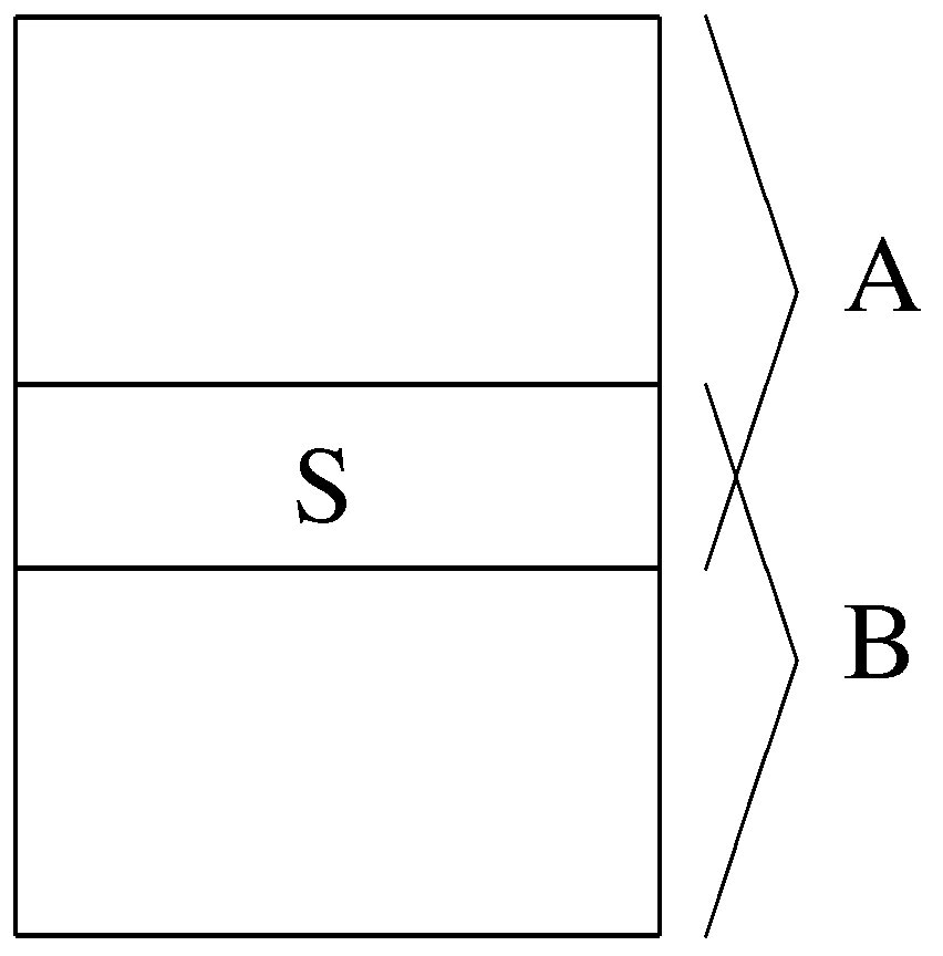
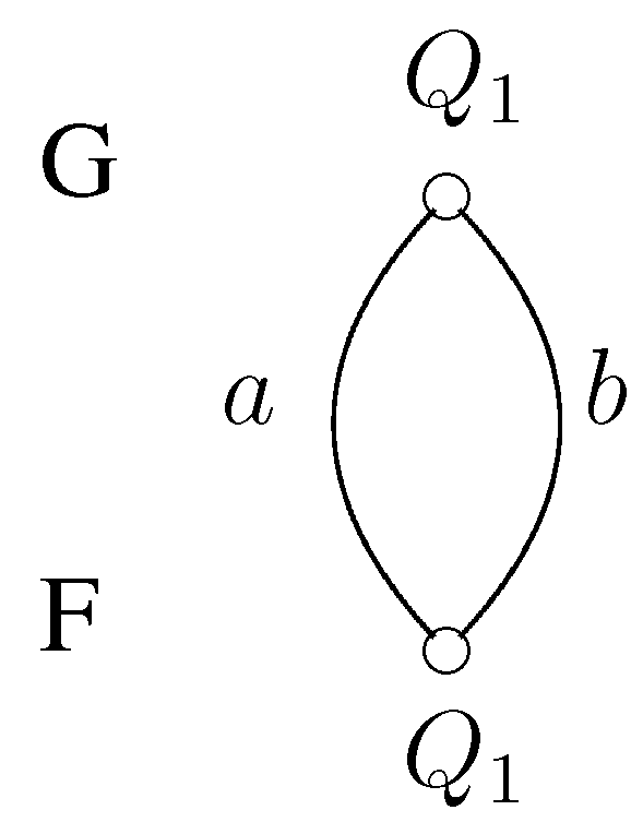
Figure 2.
Example for three-stability.
Figure 2.
Example for three-stability.

3.3. Four-Stability
We introduce the notion of four-stability: it is kind of similar to three-stability, but while a double dominated contract, e, can belong to both A and B in the three-stable sometimes, now, we put e in a fourth contract-set. Therefore, while three-stability is a more natural definition, four-stability has nicer properties and is more useful, because it is closely related to score-stability. Moreover, for path-independent choice functions, for any four-stable set, the corresponding pair is unique.
Definition 11. The choice functions of the two sides of the market are F and G. Subset S of E is four-stable, if there exists subsets A and B of E, such that and and .
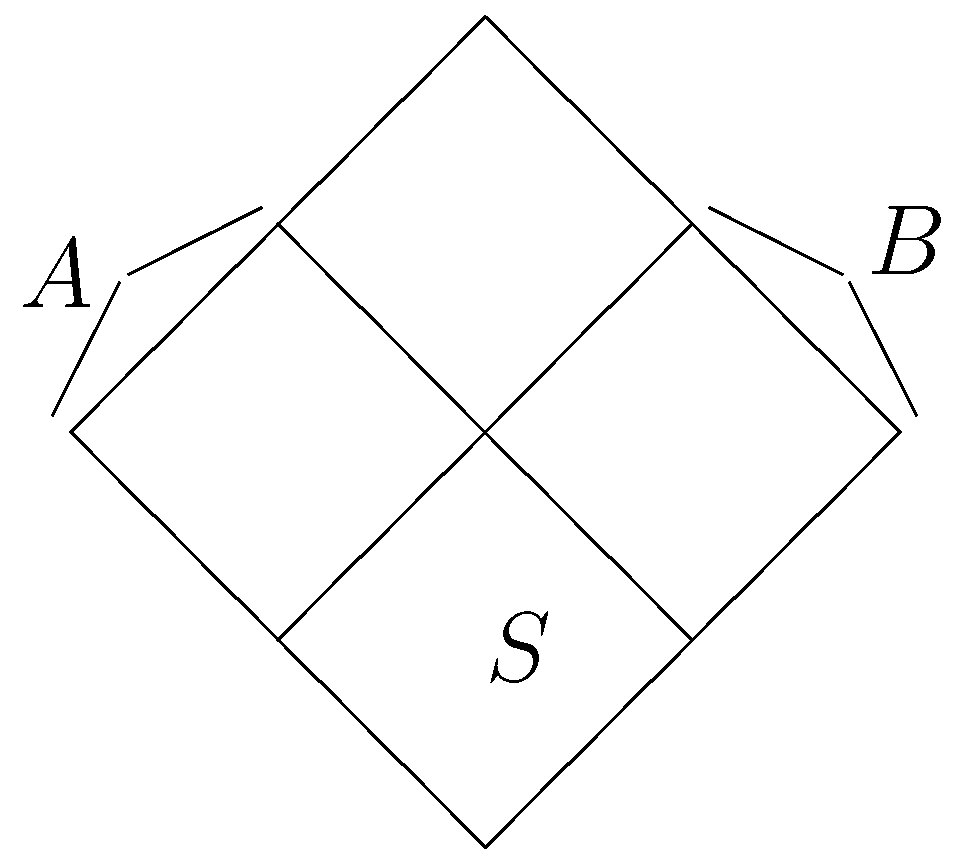
Figure 3.
Four-partition of the edge-set.
Figure 3.
Four-partition of the edge-set.

This concept is called four-stable because we partition the set E of contracts into four parts, as seen in Figure 3: S is stable; is F-dominated by S; is G-dominated by S; and the contracts in are both F- and G-dominated.
Example 7. We consider the same example as for three-stability: There are two possible contracts, a and b, and , . Now, there are three four-stable solutions:
, where , or ,
,
Remark 3. If F and G are substitutable choice functions and S is three-stable or four-stable, then .
Proof. Since and , . Similarly, implies . ☐
Statement 3. If F and G are substitutable and F is path independent, then for a four-stable set, S, there exists a unique pair.
3.4. Score-Stability
In this part, we describe the stability notion used in the Hungarian college admission scheme. For this reason, we shall call the agents colleges and applicants, and application is a synonym for contract. The mathematical model of the Hungarian college admissions system is close to stable matchings. Our model is a simplified version of the one that is used in practice. Biró, Kiselgof [9], Azevedo and Leshno [5] also examined the math behind stable score limits.
We shall generalize the model for loser-free choice functions, in particular for weighed scoring choice functions that have possible practical applications.
Assume that we have n applicants and m colleges . Let E be the set of all contracts. It is convenient to think that E is the set of edges of the bipartite graph with color classes and , where each edge, , of the graph corresponds to a contract between applicant and college . There, every applicant has a strict preference order over the colleges she applies to, and each college assigns some score (an integer between one and M) to each of its applicants. Moreover, each college, C, has a quota, , on admissible applicants. According to the law, no college can accept more applicants than its quota; moreover if an applicant, , with a certain score, , is not acceptable to some college, , then any applicant with the same or lower score has to be unacceptable for .
To determine the admissions after all information is known, each college has to declare a score limit. Let the score limits for colleges be , respectively. Each applicant will become a student at her most preferred college where she has a high enough score. More precisely, applicant is assigned to college if ( i.e., score of at is not less than threshold for ) and for ( i.e., score of at is less than the score limit, , if likes more than ). The vector of declared score limits is called a score vector. The stability notion below is defined according to the requirements of Hungarian law.
Definition 12. Score vector is valid if no college exceeds its quota with these score limits.
Score vector is critical if for every college, , either or score vector would assign more than students to (that is, no single college can decrease its score limit without exceeding its quota).
A score vector, , is score-stable if is valid and critical.
The above college admissions model determines a natural choice function for applicants and another one for the colleges. Therefore, for subset of contracts, denotes the most preferred contract from X of applicant , and is the common choice function of all applicants. Therefore, . Similarly, denotes the set of contracts that college would choose if it can select freely. More precisely, let denote the set of contracts with in X, and let declare a score limit, , such that no more than contracts from has score of at least , but either or more than contracts has a score of at least . Let be the set of all contracts in above the score limit, . Define choice function as the common choice function of all colleges, .
It is easy to see that choice function F of the applicants is path independent, but G for the colleges is not.
For example, is a typical scoring choice function; there are two equally good contracts, , and the quota is one. However, and , so it is not path independent.
3.5. Generalized Score-Stability
We can generalize the above framework, keeping the main property needed to ensure the existence of a stable solution, namely the loser-free property that allows us to extend the model in a way that is fairly generalized and has economically interesting choice functions.
Let F be direct sum of substitutable choice functions of the applicants, and G is a direct sum of loser-free, substitutable choice functions of the colleges. Every college, , has a choice function, , over the contracts involving it, and .
We say a set of applicants is feasible for college if for the contract set ; otherwise, it is infeasible. Each contract, c, has a score, .
Lemma 3. A choice function is loser-free if and only if there exists a function , such that for every set of contracts, gives the score-limit, for which the accepted contracts above the score limit are exactly the set accepted by .
Proof. If G is loser-free, the set of accepted contracts from A are all above a score limit; let the maximal score limit they reach be . On the other hand, if we have a given score limit by , no one can be missed out, while others with the same score get in; so, G must be loser-free. ☐
Let be a function, that codes the scores of the applicants: is the set of contracts above the score limit given by score vector . . Therefore, and P is antitone on the scores: if , then .
Note that for every .
There exists a score vector (a highest possible score of +1 for every college), where . From contracts above the score limit, the students choose , and contract set is acceptable for the colleges. Therefore, score vector is valid if and only if .
The score vector, , is critical if for any , the new score vector is not valid for college , or . We call stable if it is both valid and critical.
Lemma 4. If is valid, but is not, then the only college that can get an infeasible set of students at score vector is college .
Proof. The set of offered places increases at college and stays unchanged at other colleges. For applicant , if she rejected a college, , earlier (where ), she will also reject when she has more choices, so colleges other than cannot have too many students.
With score limit , the set of students going to college is ; denote it by Z. Additionally, with score limit , it is . As we have seen, , and from the substitutability, implies . ☐
Definition 13. We call a score vector -valid, if it is acceptable for college , i.e., .
The following two lemmas help to understand how the set of the valid score vectors look:
Lemma 5. Let and be two score vectors, and is -valid. For college , score limit , but for every college . Then, is also -valid.
Lemma 6. Let and be two valid score vectors, and is their pointwise minimum ( for every ). Then, is also valid.
4. Algorithms
In this section, we show algorithms to find three-stable, four-stable and score-stable allocations. As we will see, these stable solutions always exist, if F and G are substitutable (and G is also loser-free in the case of score-stability). Moreover, these algorithms give us the men-optimal/women-optimal solutions. We show a close connection between Tarski’s fixed theorem and the Gale–Shapley algorithm.
4.1. Tarski’s Fixed Point Theorem
Recall that a lattice is a partially ordered set, L, with the property that any two elements, , of L have a greatest lower bound and a least upper bound . A lattice, L, is complete if any subset, X, of L has a greatest lower bound and a least upper bound . Function from lattice L to lattice is monotone if implies for any elements, , of L.
Theorem 4 (Tarski’s fixed point theorem [10]). Let L be a complete lattice and be a monotone function on L. Then, set of fixed points of f is a nonempty, complete lattice on the restricted partial order.
If lattice L is finite in Theorem 4, there is a straightforward algorithm to find the least and greatest fixed points. Let zero be the smallest element in lattice L. Therefore, and from monotonity . Since the lattice is finite, there exists an i, where . Therefore, is a fixed point.
Statement 4. The above fixed point is the least of all fixed points of f.
Proof. Let x be an arbitrary fixed point of f. Since f is monotone, ⇒ and for every . We get that . ☐
Similarly, we can start with the greatest element one. From , we see that there is a j, such that .
This is the greatest of all fixed points of f.
4.2. Generalized Gale–Shapley Algorithm for Three-Stable and Four-Stable Sets
For three-stable sets, we can generalize the Gale–Shapley algorithm to the case where both choice functions are substitutable, but they do not have to be path independent. It is a special case of the monotone function iteration that finds a fixed point of a monotone function. The following algorithm is the same as in [6]:
Let F be the choice function of men/students, and G is the choice function of women/colleges. In the male-proposing version, let ; men choose from all contracts and propose to . Women choose and reject . In the second step, men choose from all contracts, except for the rejected ones: . They choose . The women take these contracts and the previously rejected contracts and choose from . Since G is substitutable, if a contract was rejected earlier, it will be rejected in this step, as well.
Here, this algorithm differs from the original Gale–Shapley, since there, women choose only from their current proposals. However, if G is path independent, then implies ; so, putting back already refused proposals to the choice set does not change the outcome.
A general step of the algorithm: for a given , let , and let . Define the following function, f:
We can define a partial order on pairs , if and .
Observe that f is monotone for this ordering. The iteration of this monotone function gives us a fixed pair , which corresponds to a three-stable pair . If we start our iteration from pair , we get the male-optimal matching; if we start from , we get the female-optimal one.
There is an alternative algorithm similar to the previous one:
Define function by:
If F and G are substitutable, then is monotone for order ≤, since, if B decreases, then decreases; so increases. Similarly, if A increases, then decreases.
As before, three-stable pairs are exactly the fixed points of . We start the iteration from for the men-optimal or with for the women-optimal solution.
For four-stability, we define monotone function as follows:
If are substitutable, then are monotone; therefore, is monotone for order ≤. Fixed points of are four-stable pairs , since , .
If we start the iteration of from , we get a four-stable pair with the largest possible A and smallest possible B; so, it is men-optimal. Starting pair leads to the women-optimal solution.
4.3. Algorithms for Score-Stability
In this section, we describe algorithms for the generalized score-stability, hence also for score-stability.
1. The score-decreasing algorithm: colleges start from a valid score vector (e.g., ). First, if there is a college, , that can lower its score limit without getting too many students, then will decrease its score limit to the lowest score, such that still gets a feasible set of students. Here, chooses from free students and students who prefer to their college; so, it chooses score limit . Then, we find another college, and iterate this score-decreasing step. (It is convenient to check first, then , then all colleges one-by-one. After , we return to again.) The algorithm terminates if no college wants to lower its score limit any more. As soon as no college can decrease its score limit, the score vector is stable. Let denote the stable score vector that we get by running the score-decreasing algorithm on .
Theorem 5. If stable score vector is the output of the score-decreasing algorithm with input , where is valid, then is stable and is , the maximum of all the stable score vectors that are not greater than . Consequently, is the maximum of all stable score vectors. Furthermore, is applicant-pessimal.
2. The score-increasing algorithm: colleges start with some critical score vector, (e.g., ), and keep on raising their score limits. If there is a college, , that has an infeasible set of students, then it raises the score limit to the lowest score where it becomes feasible. Therefore, it chooses . Then, another college, , increases the score limit and all colleges one-by-one. The algorithm stops if no college wants to raise its score limit. Let be the stable score vector the score-increasing algorithm outputs from input .
Theorem 6. If score vector is the output of the score-increasing algorithm with input , where is critical, then is stable, and it is the minimum of all the stable score vectors that are not less than . Consequently, is the minimum of all stable score vectors. Moreover, is applicant-optimal.
Theorem 7. The score-decreasing and score-increasing algorithms run in polynomial time; the decreasing terminates in steps, and the increasing stops in steps.
5. The Lattice Property
Tarski’s Theorem implies the following corollary for three-stability.
Theorem 8. [8] If are substitutable choice functions, then three-stable pairs form a nonempty complete lattice for partial order ≤.
Define function by:
It is straightforward to see that three-stable pairs are exactly the fixed points of f. Therefore, since f is monotone, three-stable pairs form a lattice.
A similar theorem can be proven for the four-stable pairs:
Theorem 9. If are substitutable choice functions, then the four-stable pairs form a nonempty complete lattice for partial order ≤.
Function
is monotone, and its fixed points are exactly the four-stable pairs; so, we can use Tarski’s theorem again.
5.1. Generalization of Blair’s Theorem
In this subsection, we show a lattice property of stable sets (rather than stable pairs).
Definition 14. Define a new partial order: for choice function F, let if .
Observation 1. [3] If F is substitutable and path independent, then is indeed a partial order; in particular, implies .
Blair proved the lattice property of dominating stable sets assuming the path-independent property of the choice functions [3]. As we will see in Theorem 15, if F and G are both path independent, the dominating stability, three-stability and four-stability are equivalent, so Blair’s theorem holds for each of these notions.
Theorem 10 (Blair). [3] If are substitutable, path-independent choice functions, then the dominating stable sets form a lattice for partial order .
We generalize the above lattice property for four-stability, and there is a close connection between score-stability and four-stability. Now, we require path independency on only one side.
Theorem 11 (Generalization of Blair’s theorem). If F and G are substitutable choice functions and F is path independent, then: The four-stable sets form a lattice for partial order ; If S is a four-stable set, then, there is a unique four-stable pair that corresponds to S; furthermore, if and only if .
If only one of F and G is path independent, dominating stable sets do not form a lattice. Moreover, dominating stable sets do not necessarily exist, as we have seen is SubSection 3.1.
Example 8. Given one college, , and two applicants, , and two contracts, and . The college has a quota of one, and both applicants want to go to ; so, . The dominating stable solutions are and ; however, a and b are uncomparable, since . Therefore, the dominating stable sets do not form a lattice.
Remark 4. If F and G are substitutable choice functions, but none of them is path independent, then the lattice property does not always hold for four-stability. It is also false that for stable set S there is only one corresponding pair.
Example 9. We have two contracts, a and b. The choice function is for both sides. In this situation, we have four four-stable pairs:
Now, and , but and are uncomparable. Therefore, these two sets do not have a supremum.
5.2. The Lattice of Stable Score Vectors
A graph, G, is simple if G has neither parallel edges nor loops. Therefore, between a given student and college, only one contract is permitted. In some applications, for example in the college enrollment system, the underlying graph is simple: one cannot apply to the same department, in the same year, twice. For the sake of generalizations that involve for example loser-free choice functions, the underlying graph in our model may not be simple.
Assume that F and G are substitutable choice functions and G is also loser-free. Define the following function :
Therefore, we take all contracts above score limit (this is ) and add those contracts that are not dominated by . Then, is the score limit that the colleges choose for this set.
If , then . Since is monotone, . For a greater set, gives a higher score limit; so, . Therefore, f is a monotone function, indeed.
Statement 5. If the underlying graph, , is simple, and choice functions F and G are substitutable, G is loser-free; then, score vector is stable if and only if
Tarski’s fixed point theorem implies the following corollary:
Theorem 12. If graph is simple, choice functions F and G are substitutable and G is loser-free, then the score-stable sets form a non-empty lattice.
Moreover, we can achieve a connection with four-stability for every bipartite graph.
Statement 6. If choice functions F and G are substitutable, G is loser-free and F is path independent, then the following two statements are equivalent: (i) for some score vector , such that . (ii) The contract set S is four-stable.
As a corollary of Statements 5 and 6, we get the following theorem:
Theorem 13. If choice functions F and G are substitutable, G is loser-free and the applicants’ choice function F is path independent, then every score-stable set is also four-stable. Furthermore, if we require that graph is simple, then score-stability is equivalent with four-stability.
Example 10. Figure 4 illustrates a counterexample for Theorem 13 if the underlying graph is not simple.
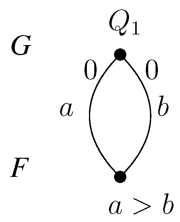
Figure 4.
A counterexample.
Figure 4.
A counterexample.

There is one college and one student, and the student applies both for math and physics, but prefers math. She achieved a zero score on both. The college has a common quota of one for these two faculties. If the score limit is one, the college accepts nobody.
If the score limit is zero, the college accepts both contracts a and b, and the applicant prefers a, so only a realizes. This is valid and stable. Therefore, the only score-stable solution is , . There are two four-stable sets: with
Stable score vectors form a lattice, even if the graph is not simple; so, a stronger version of Theorem 12 is also true:
Theorem 14. If choice functions F and G are substitutable and G is loser-free, then the score-stable sets form a non-empty lattice.
In the Appendix, we prove Theorem 14 by taking a pointwise minimum of and and starting from there. The score-decreasing algorithm terminates at stable score vector .
Remark 5. If we consider L-stable score vectors, they also form a lattice, since the permissive scoring choice function used in L-stability is also loser-free.
6. Connection between Different Stability Notions
For a given two-sided model with choice functions F and G for each side, we have defined four kinds of stability:
- Subset S of E is three-stable, if there exists subsets A and B of E, such that and , .
- Subset S of E is four-stable, if there exists subsets A and B of E, such that and and and .
- Subset S of E is dominating stable, if .
- If F is substitutable, G is substitutable and loser-free; we defined generalized score-stability in SubSection 3.5
Theorem 15. If F and G are substitutable and path independent, then S is three-stable ⇔S is four-stable ⇔S is dominating stable.
Theorem 16. If F and G are substitutable choice functions, F is path independent, (but G may not be); then, every four-stable set is three-stable.
Compared to other stability concepts, three-stability, four-stability and dominating stability are defined on every substitutable choice functions, F and G, but for score stability, we need substitutability on one side and a substitutable, loser-free function on the other side.
As we showed in Theorem 13, if choice function F is substitutable and path independent and G is substitutable loser-free, then every score-stable set is also four-stable.
Theorem 17. If F is substitutable and path independent and G is substitutable and loser-free, then every score-stable solution is three-stable.
Theorems 13, 15, 16 and 17 are summarized in Figure 5 below. In the notations, 3 stands for three-stable, 4 for four-stable, d for dominating stable and s for score-stable sets.

Figure 5.
Graphs of the connections.
Figure 5.
Graphs of the connections.
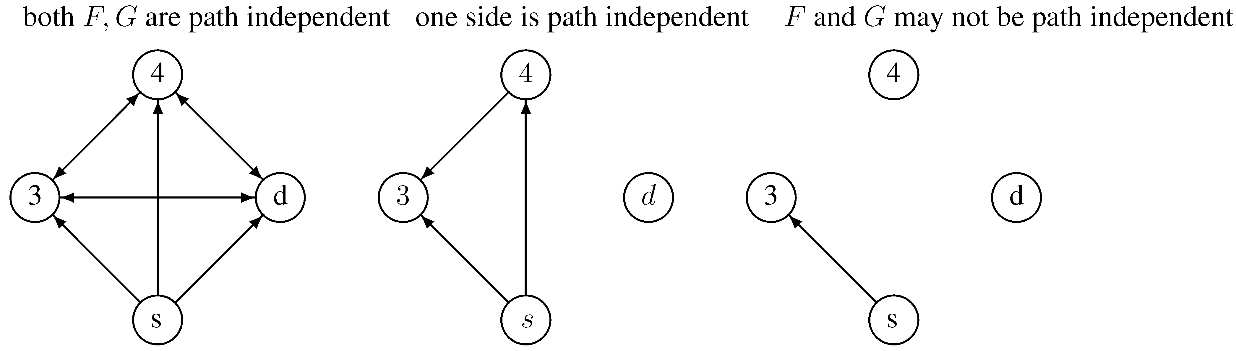
If the graph is simple: If F and G are path independent, all four properties are equivalent; If F is path independent, four-stablility is equivalent to score-stability; If F and G are not path independent, similarly to the upper picture, only score-stable ⇒ three-stable is true.
Statement 7. For all the other directions in Theorems 13, 15, 16 and 17, if one implication “if S is x-stable, then it is y-stable” does not appear in the upper diagram, then there exists a counterexample for it.
7. Conclusions
We worked with four different stability definitions: dominating stable, three-stable, four-stable and score-stable, from which the first three are rather theoretic, and score-stability can be applied to the Hungarian college admission system. All of them, except for dominating stability, can be found with simple algorithms and have some kind of lattice property, for the characteristic pairs or for the stable contract sets themselves. Moreover, under given conditions, the lattice of the four-stable and score-stable sets are the same. We used Tarski’s theorem to prove the lattice property, except for the last case: score-stability with non-simple graphs.
Acknowledgments
We thank the two anonymous referees for their remarks that helped to improve the presentation of the work. Both authors are members of the Hungarian Academy of Sciences-Eötvös Loránd University Egerváry Research Group. Research was supported by Hungarian Scientific Research Fund OTKA grant K 108383.
Conflicts of Interest
The authors declare no conflict of interest.
References
- Gale, D.; Shapley, L.S. College admissions and the stability of marriage. Am. Math. Mon. 1962, 69, 9–15. [Google Scholar] [CrossRef]
- Kelso, A.S., Jr.; Crawford, V.P. Job matching, coalition formation, and gross substitutes. Econometrica 1982, 50, 1483–1504. [Google Scholar] [CrossRef]
- Blair, C. The lattice structure of the set of stable marriages with multiple partners. Math. Oper. Res. 1988, 13, 619–628. [Google Scholar] [CrossRef]
- Aygün, O.; Sönmez, T. Matching with Contracts: The Critical Role of Irrelevance of Rejected Contracts; Mimeo, Boston College: Chestnut Hill, MA, USA, 2012. [Google Scholar]
- Azevedo, E.M.; Leshno, J.D. A Supply and Demand Framework for Two-Sided Matching Markets; Working Paper; MATCH-UP 2012; The Second International Workshop on Matching Under Preferences: Budapest, Hungary, 2012. [Google Scholar]
- Hatfield, J.W.; Milgrom, P.R. Matching with contracts. Am. Econ. Rev. 2005, 95, 913–935. [Google Scholar] [CrossRef]
- Knuth, D. Marriages Stables; Les Presses de l’Universite de Montreal: Montreal, QC, Canada, 1976. [Google Scholar]
- Fleiner, T. A fixed-point approach to stable matchings and some applications. Math. Oper. Res. 2003, 28, 103–126. [Google Scholar] [CrossRef]
- Biró, P.; Kiselgof, S. College Admissions with Stable Score-Limits. Cent. Eur. J. Oper. Res. 2013, 1–15. [Google Scholar]
- Tarski, A. A lattice-theoretical fixpoint theorem and its applications. Pac. J. Math. 1955, 5, 285–310. [Google Scholar] [CrossRef]
Appendix
Proof of Lemma 1. If , then for every , we have . Therefore, by F path independence, ; so . Consequently, .
If , then , for every ; so, from substitutability, . Thus, , which means .
By the path independence of F, we have ⇒ ☐
Proof of Lemma 2. We have seen that is monotone; hence .
If , then ; so by the path independency.
Therefore, ; hence . This means S dominates any , i.e., . ☐
The proof of statement 3 is included in the proof of Theorem 11.
Proof of Lemma 5. If is a student of when the score vector is ( i.e., ), then can leave at if she does not reach or got a better opportunity at another college.
If student does not go to college at the score vector, , (), then she will not go to under score vector , because if does not reach , then she does not reach the higher limit, . If reaches , but chooses better college instead, since , she will stay in college . Therefore, the set of students assigned to with is the subset of the set of students going to under . The choice function, , of college is substitutable. Therefore, is valid; then, a subset of it is also valid. Therefore, is -valid. ☐
Proof of Lemma 6. Let the set of contracts above score vectors and be and . Then, . Suppose that for college . Since , from substitutability . Considering the set of contracts of college , , i.e., accepts the same set of contracts with score vector as with . Therefore, . Since G is substitutable, if a set is valid, then its subset is also valid. so . For a smaller set, ; so, is also valid for college .
In other words, if we change the score limit from to , college keeps its score limit, while other colleges may decrease it. Applicants may leave , but no new students will arrive to ; so, score limit is -valid. We can use the same argument for every college; therefore is valid. ☐
In the proofs of Theorems 5 and 6, we use the alternative versions of the score-decreasing/increasing algorithms, where in every step, a college decreases/increases its score limit only by one. These modified algorithms also find stable solutions, as one step of the score decreasing or score increasing can be regarded as several steps of this modified algorithm. From Lemma 5, if score vector is valid and is also valid, then for every , is valid (it is -valid, because is valid, and valid for other colleges, because t is valid). ☐
From the maximal/minimal property of the output solution, we see that the output of the algorithm does not depend on what order by which the colleges modify their score limits. Note that these algorithms may use steps, for example, if we start decreasing from ), but only is a stable score vector.
Proof of Theorem 5. From the algorithm, the fact that no college can decrease its score limit implies that is a stable vector.
Suppose that there exist a stable score vector , where . Therefore, and , and for some i. Define the set:
The algorithm starts from and ends in ; so, there is a step, when the score vector leaves T: from score vector , we move to . Since this step is possible, both and are valid score vectors. We know that . Using Lemma 6, both and are valid; so, their minimum is also valid. Therefore, is stable, and it can be reached from by lowering the score limit of . Therefore, is not critical, hence it cannot be stable; a contradiction.
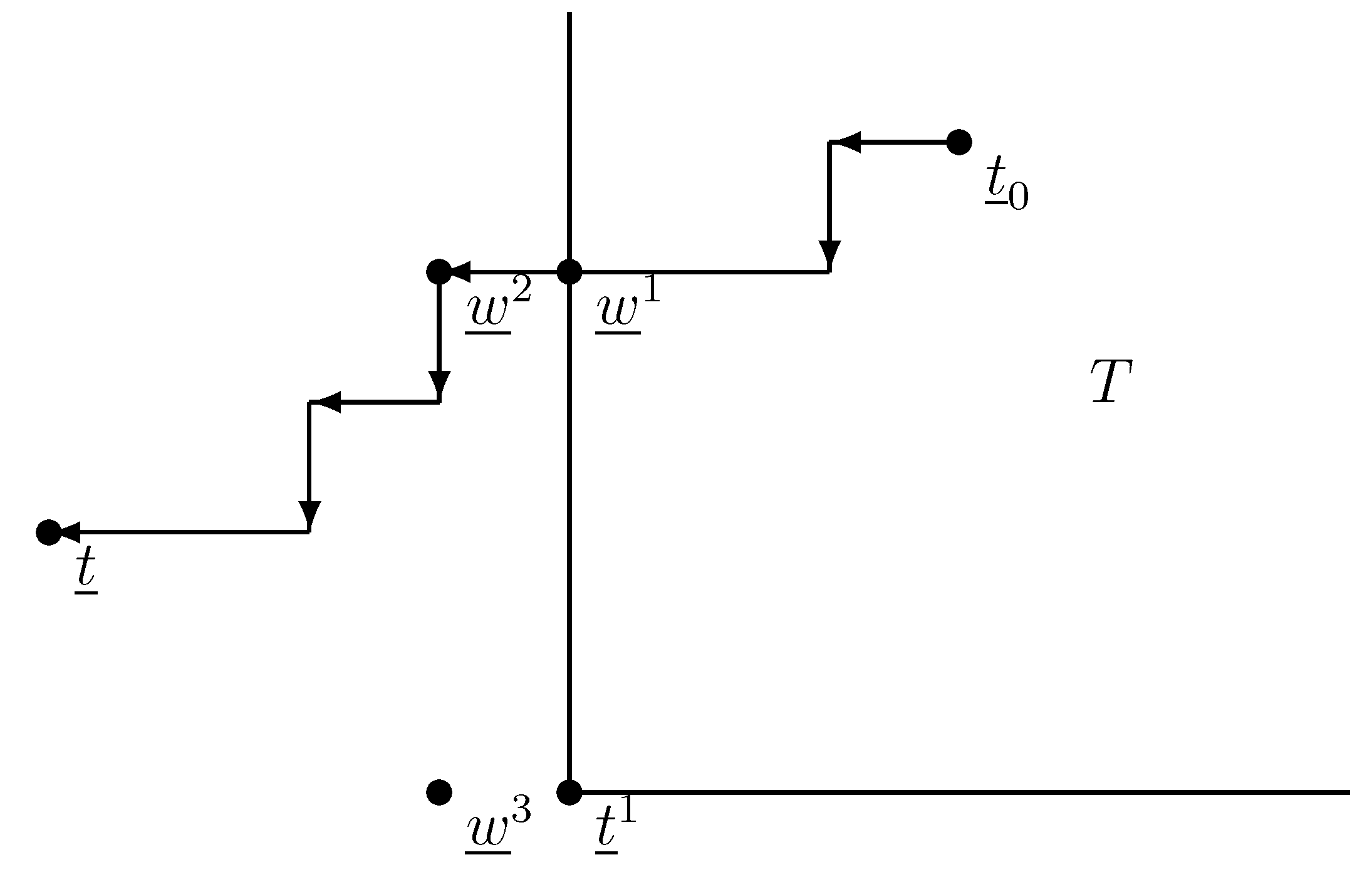
Since every stable score vector are less than or equal to , the biggest of all stable score vectors is . Every student is accepted by fewer colleges than in any other stable admissions; so, is applicant-pessimal. Figure 6 is showing a possible layout. ☐
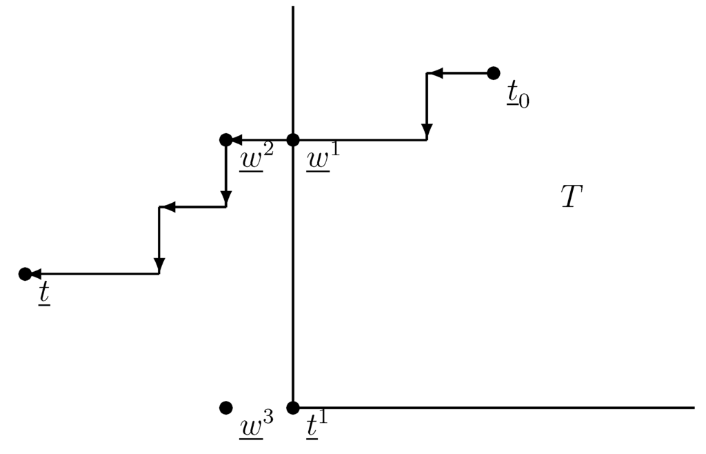
Figure 6.
Score-decreasing algorithm.
Figure 6.
Score-decreasing algorithm.
Proof of Theorem 6. It follows from the algorithm that is valid. Suppose that it is not stable, i.e., there is a college, , such that is still valid.
If , look at the step where college raises its score from to , moving from score vector to .
Since the score limits in the algorithm always increase, and ; therefore, . We can use Lemma 5: score limit is valid, so is also -valid. However, then, the algorithm would not have increased to ; a contradiction; Therefore, is stable.
If , since is critical, the score vector is not valid for . From , we get that . Using Lemma 5 again, if was valid, then would be -valid. Therefore, is not valid; therefore, is indeed stable.
To show that is minimal, suppose that there is a stable score limit, , such that , but , i.e., for some j. Let:
Since , but , there is a step such that when we leave , we move from to . There is a college, , where . For other colleges, ; so, by Lemma 5, was -stable. Therefore, does not want to increase its score limit.
Therefore, is the smallest of all stable score vectors; so, every student gets accepted at as many colleges as possible, and they choose what is best for them. Therefore, is applicant-optimal. Figure 7 is showing a possible layout. ☐
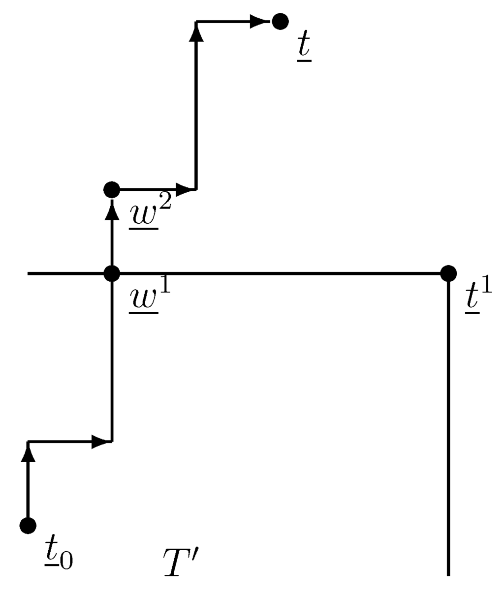
Figure 7.
Score-increasing algorithm.
Figure 7.
Score-increasing algorithm.

Proof of Theorem 7. In this proof, we return to the algorithm versions where colleges increase/lower their score limits as much as they can. We call the set of realized contracts at some score vector enrollment.
Each of the n students can go to one of the m colleges or remain unmatched. Therefore, there are at most possible enrollments. In the score-decreasing algorithm, the applicants always change to better. In the score-increasing algorithm, the students’ positions get worse. Therefore, we cannot return to an earlier enrollment in these algorithms.
If we order all enrollments according to the applicants’ preference order, the longest chain contains enrollments. It goes from “everyone gets the best college” to “everyone gets the worst college”. In the score-decreasing algorithm, college may lower its score limit without changing the enrollment, taking the same students as before. If all m colleges do the same, we get the minimal score vector for that given enrollment; next time it came to college , it has to change to a different enrollment or stop. Therefore, in the algorithm, there can be at most m consecutive steps without changing the enrollment. Therefore, the number of steps is .
In the score-increasing algorithm, every step will change the enrollment; hence, if increase its score limit, the set of students going to was infeasible before this step and feasible after the step. Thus, the number of steps is .
☐
Proof of Theorem 11. (i) First, we show that for any given stable set S there is a unique four-stable pair .
Suppose that there are two different stable pairs for S: and .
We can assume that there exists a b for which , but . Since , it follows that . Moreover , but , because .
By , we get ; hence .
We know that and .
Since F is substitutable, contains both sets, ; so, .
From , we get ; so, .
Using that F is path independent, from Theorem 3, . Therefore, ; a contradiction.
Let S and be two different stable sets. Let four-stable pairs and correspond to stable sets S and , respectively.
(ii) ⇒.
From the ordering of the four-stable pairs, and ; so, .
Since F is path independent, from , we get that .
(iii) , ⇒ .
Suppose that . Consequently, , such that , but . From Lemma 2, ; so:
⇒⇒
⇒⇒
We know that ; therefore, . Since F is path independent, ; hence ; a contradiction.
Similarly, from , we get by the monotonicity of and ; hence .
(iv) The stable sets form a lattice.
We have seen that there is an order preserving bijection between the stable sets and stable pairs. As stable pairs form a lattice, stable sets do, as well. ☐
Proof of Statement 5. Let be the set of contracts that F prefers to . In other words, ; therefore, . (See Figure 8.)
Suppose is a fixed point. Let , and we use that: . From this,
Since , we get that , and since G is substitutable, . Therefore, ; so, is valid.
To prove that is critical, assume that college lowers its score limit by one. Let
. Then, at college , the accepted increases with some contracts.
Now, we use that the graph is simple. If , then applicant will also be accepted under . If is not accepted at college with score vector , but she has a score of at least , then she will go to if and only if , because she got only one new chance. Therefore, .
Other colleges cannot have new students; so, they stay valid.
From , the scoring function, , for college chooses score limit ; therefore, it also chooses from . Therefore, is not valid.
Now, assume that is valid and critical. Therefore, ; so, accepts contracts in (because contracts in J do not reach score limit ). Therefore, .
As before, . Function P is antitone; so
. Since is monotone, ; so, . As is critical, is infeasible for college ; so, , too, and we get . This is valid for every college; therefore, .
We did not use that is simple in the second direction and in the “valid” part of the first direction; so, these parts remain true for general bipartite graphs. ☐
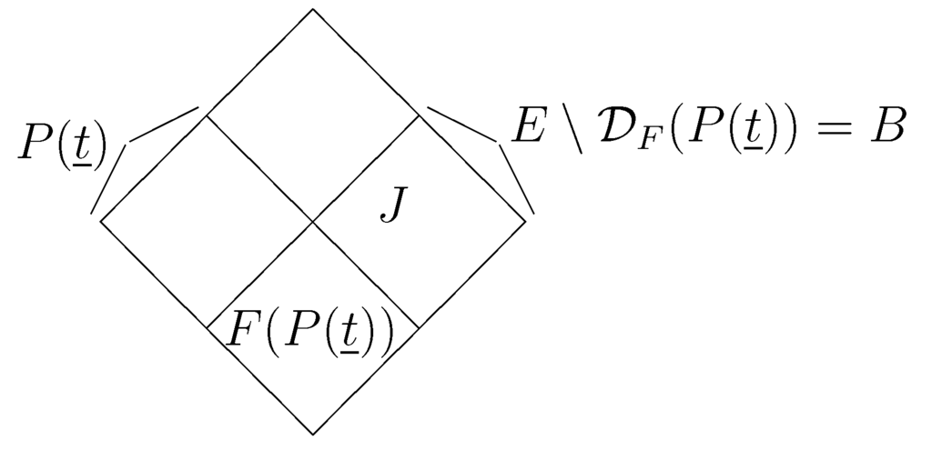
Figure 8.
Four-partition.
Figure 8.
Four-partition.

Proof of Statement 6. (i)⇒ (ii) If is a fixed point, , then let
As we have seen in the proof of Statement 5, ; so, .
This gives . From the contracts outside B, the set, B, must dominate contracts under score limit , since if colleges do not accept contracts from J, then they will not accept other contracts with the same or lower scores. (It cannot happen that for some college, , all contracts in J have a score of or less and some has a score of , because in that case, would have chosen and would not be stable.) Therefore, . Therefore, .
Since F is path independent and , we get that .
From Lemma 2, ; so, S is indeed four-stable.
(i)⇐ (ii)
If S is four-stable, then there exists , such that . Let the score limit be . We want to know what is. It is sure that , because , and since and , so .
Since , substitutability implies that dominated contracts will not be chosen from , since . Therefore, . Then, . From the path-independent property, .
Using Lemma 2 again, , and ; therefore, is a fixed point. ☐
Proof of Theorem 14. We know from Theorems 5 and 6 that there exist a greatest and a least stable score vector. Let and be two arbitrary stable score vectors. We want to show that they have a join and a meet. Using Lemma 6, is valid. Let us start the score-decreasing algorithm from ; from the algorithm, we get a stable score vector, . From Theorem 5, is the biggest among all the stable score vectors smaller than or equal to . Therefore, , because for every stable vector, such that , ; therefore, .
We finish by showing the existence of . There exists a common upper bound of and , for example . Since the lattice is finite, there has to be at least one least common upper bound. Suppose there exist two least common upper bounds: and . Since is a lower bound of and , ; similarly, . Therefore, we found a common upper bound of and smaller than a; a contradiction. ☐
Proof of Theorem 15. Three-stable ⇒ dominating
There are A and B, such that . From Lemma 1, . The same goes for ; so, . Their union is
.
Additionally, S does not dominate itself; so, .
Dominating ⇒ four-stable
We know that . Let and .
, so . From Lemma 2, . Similarly, . With this pair, S is four-stable.
Four-stable ⇒ three-stable
There exists subsets A and B of E, such that and , and .
Let and .
Now, , , and from Lemma 2, . From Lemma 1, , ; so, with the pair, S is three-stable. ☐
Proof of Theorem 16. In the third part of the proof of Theorem 15, we did not use that G was path independent. ☐
Proof of Theorem 17. Let be the enrollment realized from stable score vector . Define A as the set of contracts above score vector . Let B be the union of S and the set of contracts under score limit .
From all the accepted contracts above score vector , the applicants choose contract set S; so, . If colleges choose from contract set B, just like from all contracts, they would set score limit to ; so, . It is easy to see that ; therefore, S is three-stable. ☐
Proof of Statement 7. In Figure 2 and Figure 4 and in the following Figure 9 to Figure 13, the upper nodes symbolize the colleges, the lower nodes the applicants and the edges between them are the possible contracts. If we write to a node, that means the given applicant prefers contract a to b. In all examples, every student gets a score of zero everywhere, except in Figure 13, where contract b has a score of one; so, b is better for the college.
If a node has only one incident edge, it always chooses that, if it is available.

Figure 9.
Example graph 3.
Figure 9.
Example graph 3.
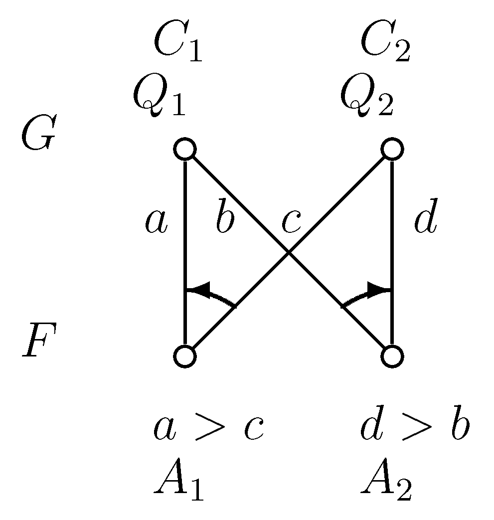

Figure 10.
Example graph 4.
Figure 10.
Example graph 4.
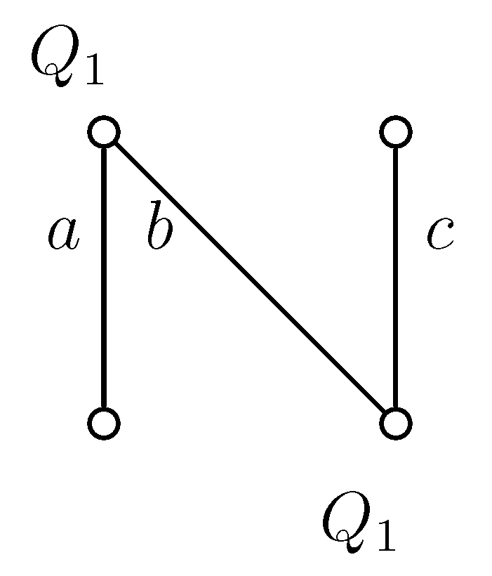

Figure 11.
Example graph 5.
Figure 11.
Example graph 5.
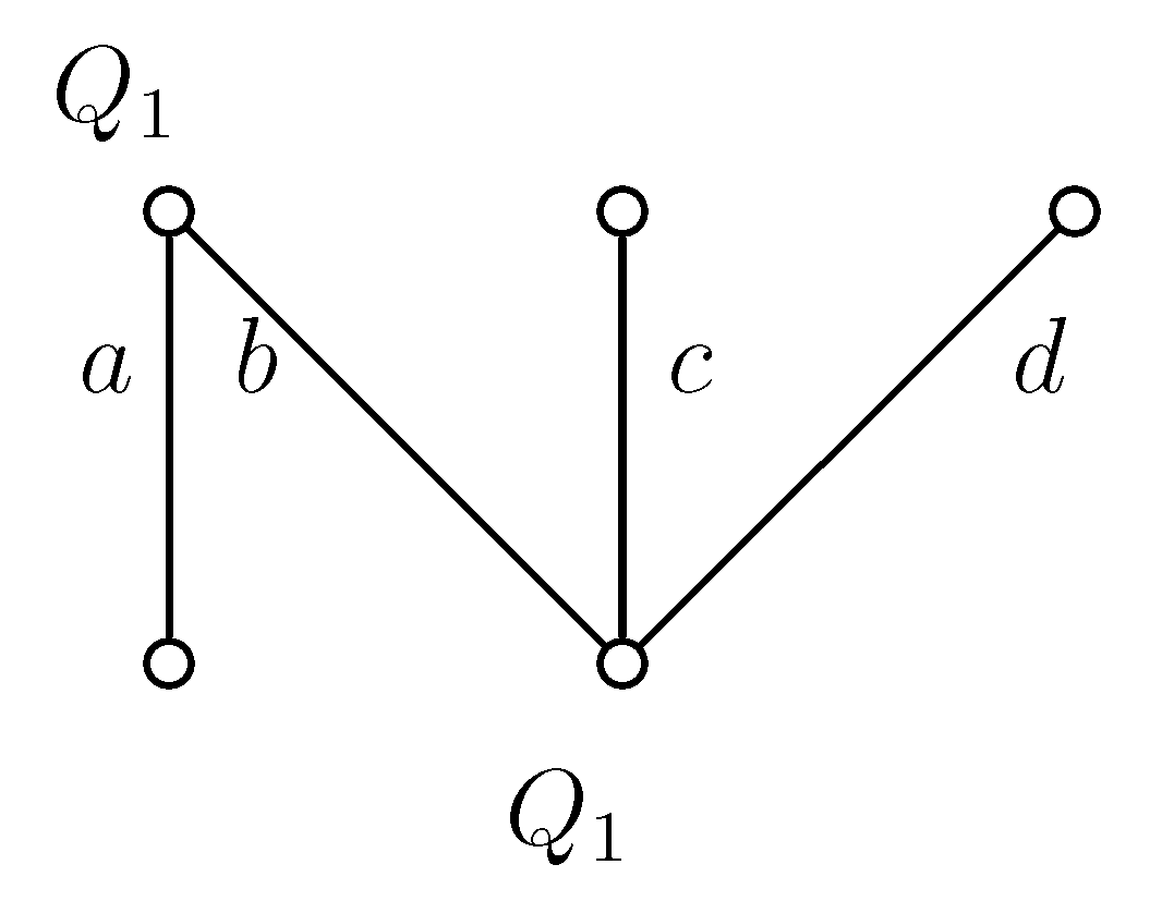
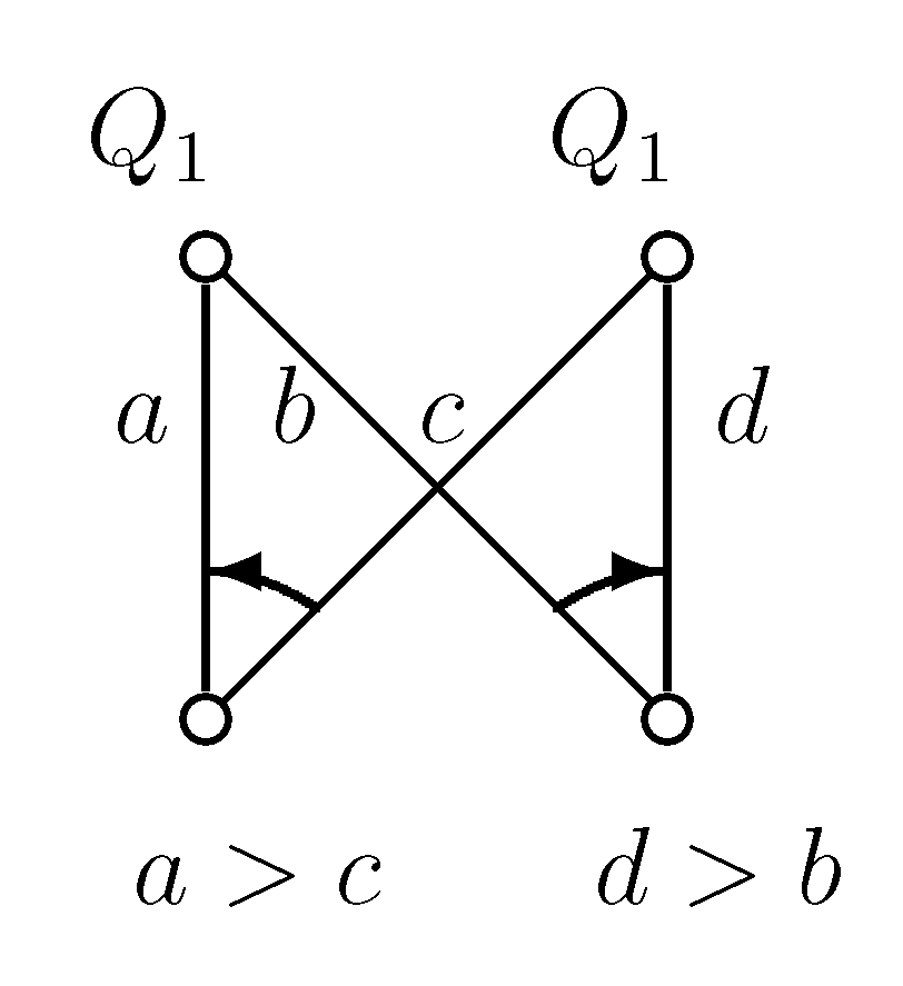
Figure 12.
Example graph 6.
Figure 12.
Example graph 6.


Figure 13.
Example graph 7.
Figure 13.
Example graph 7.
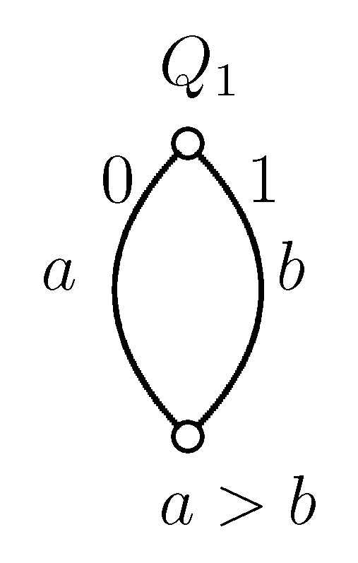
Table 1 describes the choice functions, usually as a direct sum of the choice functions of individual colleges/applicants. Notation means a college chooses from equally good contracts a and b and its quota is one. We use the abbreviation “path ind." for path independence. Table 2 shows the stable sets for each notion for the seven examples.

Table 1.
The choice functions for the seven examples.
| Figure | Simple | Path ind. | Path ind. | ||
|---|---|---|---|---|---|
| 2 | no | no | no | ||
| 4 | no | yes | no | ||
| 9 | yes | yes | no | ||
| 10 | yes | no | no | ||
| 11 | yes | no | no | ||
| 12 | yes | yes | no | ||
| 13 | no | yes | yes |
Table 2.
Stable sets in case of different stability notions.
| Figure | Three-Stable | Four-Stable | Dominating Stable | Score-Stable | Fixed |
|---|---|---|---|---|---|
| 2 | ∅ | ∅ | ∅ | ||
| 4 | |||||
| 9 | |||||
| 10 | |||||
| 11 | |||||
| 12 | |||||
| 13 |
© 2014 by the authors; licensee MDPI, Basel, Switzerland. This article is an open access article distributed under the terms and conditions of the Creative Commons Attribution license (http://creativecommons.org/licenses/by/3.0/).