Graph Extremities Defined by Search Algorithms

Abstract

Graph search algorithms have exploited graph extremities, such as the leaves of a tree and the simplicial vertices of a chordal graph. Recently, several well-known graph search algorithms have been collectively expressed as two generic algorithms called MLS and MLSM. In this paper, we investigate the properties of the vertex that is numbered 1 by MLS on a chordal graph and by MLSM on an arbitrary graph. We explain how this vertex is an extremity of the graph. Moreover, we show the remarkable property that the minimal separators included in the neighborhood of this vertex are totally ordered by inclusion.

1. Introduction

Various properties that identify a vertex as an extremity of a graph have long been exploited in both graph theory and the design of efficient graph algorithms. The endpoints of a path, for example, are its two extremities; leaves are the extremities of a tree. Because this simple notion has proved very useful in dealing with trees, graph theorists have endeavored to extend it to broader graph classes.

For chordal graphs (graphs with no chordless cycle of length greater than 3), extremities were defined as the simplicial vertices (a vertex is simplicial if its neighborhood is a clique), concurrently by Dirac [1] and by Lekkerkerker and Boland [2]. This concept led to efficient recognition algorithms for chordal graphs, based on the characterization of Fulkerson and Gross [3], who showed that a graph is chordal if and only if it has a simplicial elimination scheme, which repeatedly finds a simplicial vertex and removes it from the graph. This process defines an ordering α on the vertices, called a perfect elimination ordering (peo for short).

To compute a peo efficiently, Rose, Tarjan and Lueker [4] introduced Algorithm LexBFS (Lexicographic Breadth-First Search). LexBFS finds a peo in a single linear-time pass if the input graph is chordal, numbering the vertices from n to 1. Thus the vertex numbered 1 by LexBFS is a simplicial vertex (we will say that LexBFS ends on a simplicial vertex).

Tarjan and Yannakakis [5] later simplified LexBFS into MCS (Maximum Cardinality Search), which likewise finds a peo in a chordal graph and thus ends on a simplicial vertex. Both algorithms work by numbering the vertices from n to 1. They maintain, for each unnumbered vertex, a label which corresponds to the set of already numbered neighbors. At each step, a vertex of maximum label is chosen to be numbered next. (LexBFS and MCS are given in Section 3.) These algorithms, which are graph search algorithms, have thus been specifically designed to find an extremity in a chordal graph. As we will explain in Section 2, both LexBFS and MCS actually find a special kind of simplicial vertex.

For special classes of non-chordal graphs, search algorithms have been proved to define other forms of extremities: Dahlhaus, Hammer, Maffray and Olariu [6] used MCS to find a domination elimination ordering on HHD-free graphs; on AT-free graphs, Corneil, Olariu and Stewart [7] defined dominating pairs of vertices, and used LexBFS to find such a pair efficiently [8], as the vertex numbered 1 by LexBFS belongs to a dominating pair, and a second pass of LexBFS will find a second such vertex.

Results have also been proved on LexBFS for powers of graphs: Brandstädt, Dragan and Nicolai [9] show that any LexBFS-ordering of a chordal graph is a common perfect elimination ordering of all odd powers of this graph. (see also e.g. [10] on distance-hereditary graphs).

In view of these results, we will now focus our attention on a broader spectrum of search algorithms.

Corneil and Krueger [11] introduced MNS (Maximal Neighborhood Search), as an algorithm which encompasses both LexBFS and MCS, and also computes a peo if the graph is chordal. Berry, Krueger and Simonet [12] extended the family of search algorithms by defining a generic algorithm MLS (Maximal Label Search). Algorithm MLS has two input variables: a graph and a labeling structure describing a set of labels and a partial order on this set. Thus MLS defines a family of search algorithms, each different labeling structure defining a search algorithm. LexBFS and MCS for example are obtained as instances of MLS by choosing specific labeling structures, which are given in Section 3. [12] further showed that the set of orderings of the vertices of a given graph computable by MLS (with all possible labeling structures) is equal to the set of orderings computable by MNS, which ensures that MLS always finds a peo if the graph is chordal.

In this paper, we investigate the extremities which the MLS family of algorithms define as vertex number 1. Our aim is to contribute elements which can help in the design of graph algorithms, in particular for exploiting structural properties of the input graph.

The paper is organized as follows:

• In Section 2, we give some basic graph notations which we use throughout, and then discuss chordal graphs and their extremities in further detail, explaining how minimal separators can help refine the notion of simplicial vertex.
• We then go on to present minimal triangulations and their relationship with search algorithms. Section 3 gives the general MLS search algorithm, as well as specific instances of MLS such as LexBFS and MCS.
• After these sections which summarize and explain previous results, we examine in Section 4 the specific structure of the minimal separators included in the neighborhood of the vertex labeled 1 by search algorithms, and also discuss the fashion in which these algorithms number the connected components defined by these separators.
• In Section 5, we specify what kind of extremity this vertex numbered 1 is, depending on what kind of labeling structure is used.
• Section 6 examines the special properties exhibited by LexBFS.
• In Section 7, we discuss the specific orderings defined by MLS and MLSM.
• In Section 8, we examine the problem of deciding whether a given vertex is the number 1 vertex of an MLS execution.
• We conclude in Section 9.

2. Notations and Previous Results

We will begin this section with a few notations, then go on to discuss minimal separation, chordal graphs and minimal triangulation.

2.1. Basic definitions and notations

All graphs in this work are undirected and finite. A graph is denoted $G=(V,E)$, with $n=\left|V\right|$, and $m=\left|E\right|$. The subgraph of G induced by the subset A of vertices is denoted $G\left(A\right)$. The neighborhood of a vertex x in G is denoted $N_G\left(x\right)$. The closed neighborhood is $N_G\left[x\right]=\left\{x\right\}\cup N_G\left(x\right)$. The neighborhood of a set of vertices A is $N_G\left(A\right)={\cup }_{x\in A}{N}_G\left(x\right)-A$, and $N_G\left[A\right]=A\cup N_G\left(A\right)$ (we will omit subscript G when the graph we work on is clear from the context.)

A clique is a set of pairwise adjacent vertices. A module is a subset X of vertices which share the same external neighborhood: $\forall x,y\in X,N\left(x\right)-X=N\left(y\right)-X$.

A graph is connected if for any pair $\{x,y\}$ of vertices, there is a path from x to y. When a graph is not connected, the maximal connected subgraphs are called the connected components of the graph.

An ordering α on the set V of vertices is a one-to-one mapping from $\{1,2,...,n\}$ to V. In every figure of this paper showing an ordering α on V, a vertex x will be named by its number ${\alpha }^{-1}\left(x\right)$. To simplify notations, we will sometimes refer to vertex $\alpha \left(1\right)$ as simply 1.

Throughout, for any integers $i<j$, $[i,j]$ will denote the set of integers $\{i,i+1,..,j\}$.

2.2. Minimal separators and chordal graphs

A notion which is central to chordal graphs and their extremities is that of minimal separation:

Definition 2.1 A subset S of vertices of a connected graph G is called a separator (or sometimes a cutset ) if $G(V-S)$ is not connected. A separator S is called an $ab$-separator if a and b lie in different connected components of $G(V-S)$, a minimal $ab$-separator if S is an $ab$-separator and no proper subset of S is an $ab$-separator. A separator S is a minimal separator , if there is some pair $\{a,b\}$ such that S is a minimal $ab$-separator.

Alternately, S is a minimal separator if and only if $G(V-S)$ has at least 2 connected components $C_1$ and $C_2$ such that $N\left(C_1\right)=N\left(C_2\right)=S$, and S is a minimal separator for any $\{x,y\}$ with $x\in C_1$ and $y\in C_2$.

Example 2.2 In Figure 1, the minimal separators of the graph are: $\{b,c\},\{c,d\},\{b,f\}$. Minimal separator $\{b,c\}$ defines connected components $\{e,f\}$ and $\{a,d,g,h\}$. In Figure 2, the minimal separators are: $\left\{b\right\},\{b,d\},\left\{e\right\}$. Note how minimal separator $\left\{b\right\}$ is included in minimal separator $\left\{b\right\}$, which minimally separates vertices $\{e,f,g\}$ from vertices $\{a,c,d,h\}$, while minimal separator $\{b,d\}$ minimally separates vertices $\{a,c\}$ from vertex h.

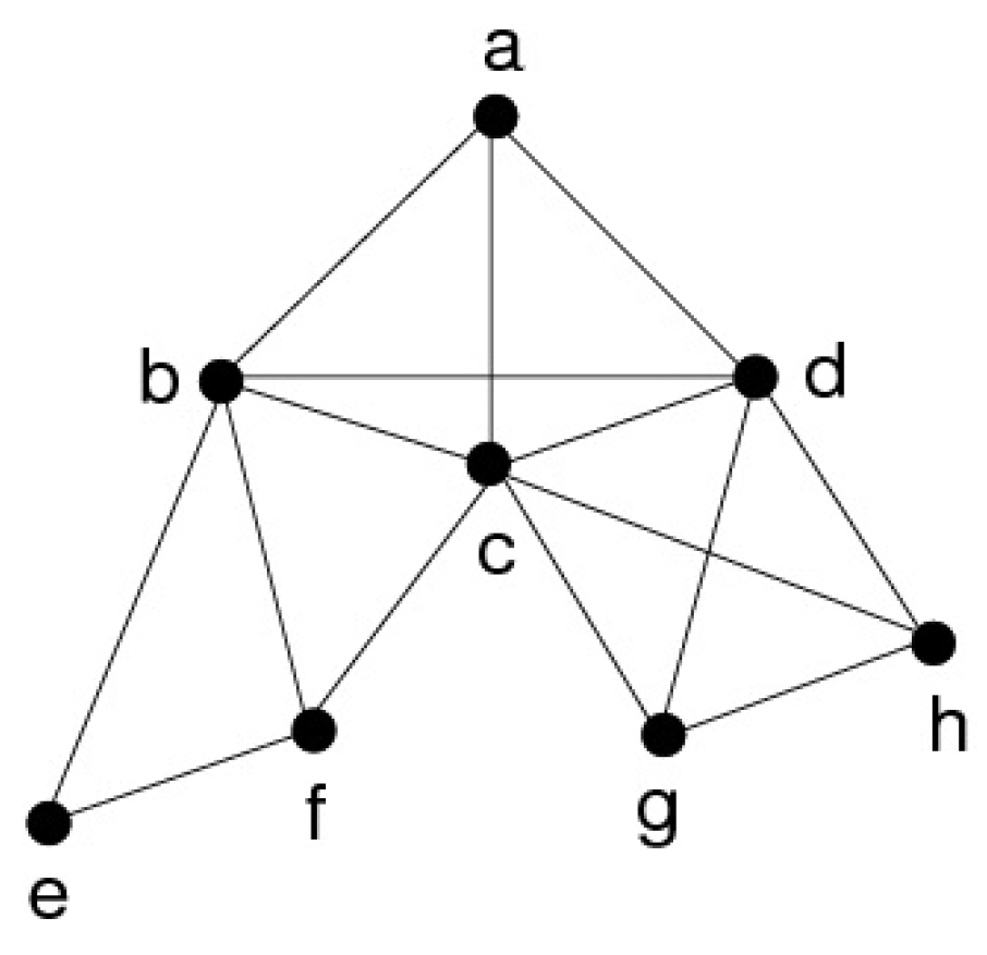
Figure 1. Chordal graph $H_1$ with set of minimal separators $\left\{\right\{b,c\},\{c,d\},\{b,f\left\}\right\}$. The substars of a are $\{b,c\}$. The moplexes are $\{g,h\}$ and $\left\{e\right\}$. Vertex a is simplicial but does not belong to a moplex. and $\{c,d\}$.

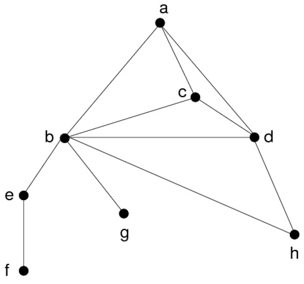
Figure 2. Chordal graph $H_2$ with set of minimal separators $\left\{\right\{b\},\{b,d\},\{e\left\}\right\}$. $\{a,c\}$ is a moplex.

Dirac [1] introduced the concept of minimal separator in order to characterize chordal graphs as the class for which every minimal separator is a clique. This notion was concurrently (though implicitly) used by Lekkerkerker and Boland [2], as they defined the notion of substar: the substars of a vertex x are the minimal separators included in the neighborhood of x. [2] characterized chordal graphs as the graphs for which every substar of every vertex is a clique. We will see later on in this paper that the notion of substar will help us refine some notions of extremities.

Definition 2.3 Let $G=(V,E)$ be a graph, let x be a vertex of V, let $\left(C_i\right)$ be the connected components of $G(V-N[x\left]\right)$. The substars of x are the elements of $\left(N_G\left(C_i\right)\right)$.

Property 2.4 The substars of x are the minimal separators included in $N_G\left(x\right)$.

Example 2.5 In Figure 1, the connected components of $G(V-N[a\left]\right)$ are: $C_1=\{e,f\}$ and $C_2=\{g,h\}$. $N\left(C_1\right)=\{b,c\}$, $N(C_2=\{c,d\}$, thus the substars of vertex a are $\{b,c\}$ and $\{c,d\}$.

Berry and Bordat [13] refined the notion of simplicial vertex with new kind of extremity. This is a group of pairwise adjacent vertices, which they call a moplex:

Definition 2.6 [13] Let X be a set of vertices of a graph G. X is a moplex of G if X is a clique and a module of G whose neighborhood is a minimal separator.

The vertices of a moplex are in some sense equivalent, because they share the same external neighborhood (i.e., they form a module); thus they also share the same substars. Moreover, this common neighborhood is a minimal separator, which means that there is one largest substar (which includes all the other substars). Note that a moplex X may contain a single vertex x; in this case we will call X a trivial moplex.

In Figure 1, $\{g,h\}$ is a moplex, e is a (trivial) moplex. In Figure 2, $\{a,c\}$ forms a moplex, with substars $\left\{b\right\}$ and $\{b,d\}$.

The notion of moplex strengthens the notion of simplicial vertex, as in a chordal graph any vertex of a moplex is simplicial, whereas in some chordal graphs, there may be simplicial vertices which do not belong to any simplicial moplex. In Figure 1, for example, a is simplicial but does not belong to a moplex.

[13] showed that LexBFS always ends by numbering consecutively all the vertices of a moplex, even on a non-chordal graph. It follows from [14] that MCS run on a chordal graph has the same property.

This notion of moplex is important in the context of this paper, as our aim is to investigate exactly which kinds of extremities the MLS algorithms define.

2.3. Extremities defined by minimal triangulations

For arbitrary graphs, extremities have been yielded by algorithms which compute a minimal triangulation of a graph (a chordal graph obtained from this graph by adding an inclusion-minimal set of edges).

Obviously, one can use the characterization of Fulkerson and Gross to embed a graph into a chordal graph by repeatedly choosing a vertex, adding to its neighborhood every edge whose absence violates the simpliciality condition, and then removing the vertex from the current graph, thus simulating a simplicial elimination scheme and a perfect elimination ordering α on the vertices. This process (called the elimination game) defines a triangulation of G denoted $G_{\alpha }^{+}$. Ohtsuki, Cheung and Fujisawa [15] proved that to compute such a triangulation which is minimal, one has to use a special ordering on the vertices, called a minimal elimination ordering (meo for short). [15] showed that an ordering is a meo if and only if at each step of the simplicial elimination game, a special vertex is chosen. Since they did not give these vertices a name, and since the notion is of importance to our work, we call these vertices OCF-vertices. Let us restate their characterization using the notations previously defined in this paper:

Definition 2.7 [15] A vertex x in $G=(V,E)$ is an OCF-vertex of G if for every pair $\{y,z\}$ of distinct non-adjacent neighbors of x in G, y and z belong to some common substar of x.

[15] showed that in any non-clique graph, there is an OCF-vertex.

Example 2.8 In Figure 3, a is an OCF-vertex: its substars are $\{b,c\}$ and $\{c,d\}$, and only edges $bc$ and $cd$ are missing in the neighborhood of a.

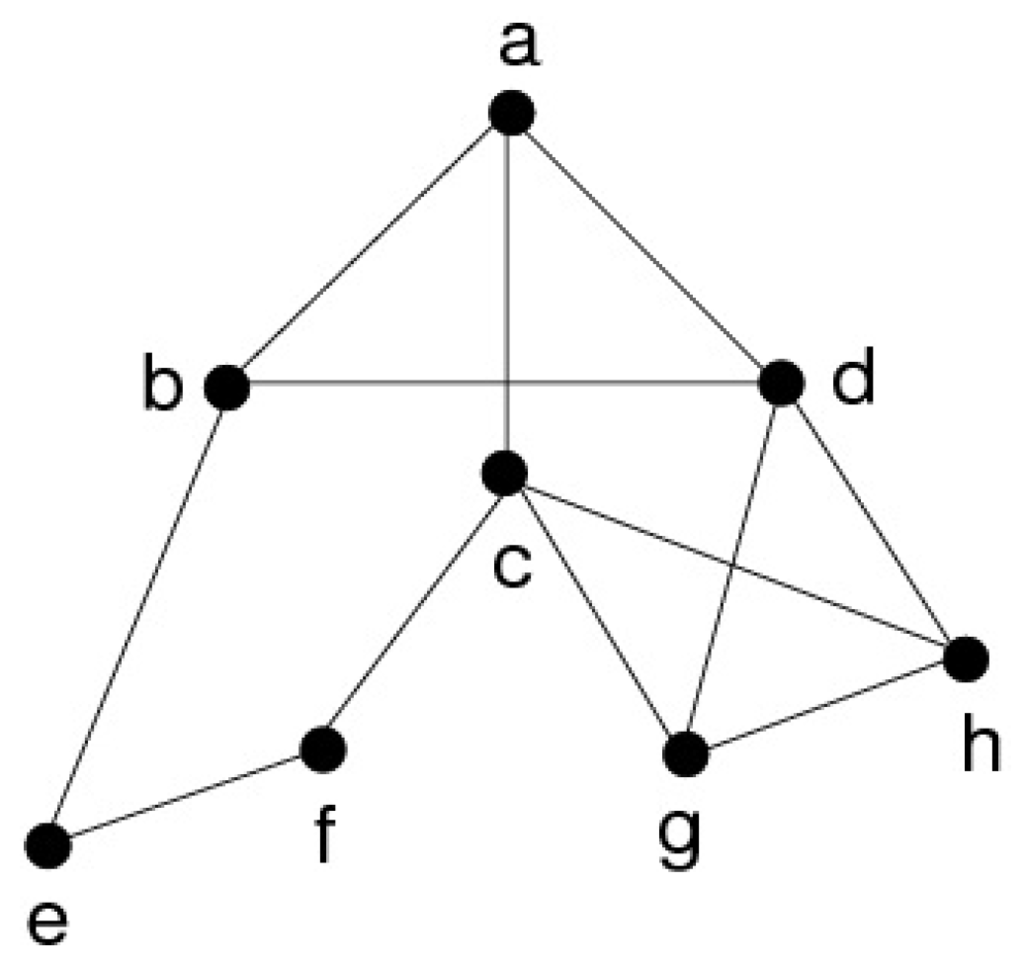
Figure 3. A non-chordal graph G. The set of minimal separators of G is: $\left\{\right\{b,f\},\{c,d\},$ $\{c,e\},\{a,d,e\},\{a,d,f\},\{a,b,g,h\},\{a,e,g,h\},\{a,f,g,h\}\}$.

An OCF-vertex x can be viewed as an extremity of an arbitrary graph: if x is chosen first in an instance of the elimination game, x will be a simplicial vertex of the corresponding minimal triangulation. The notion of moplex, (the definition of which is not restricted to chordal graphs), also strengthens the notion of OCF-vertex, since all the vertices of a moplex are OCF-vertices, but some OCF-vertices may not belong to a moplex.

In Figure 3, a is an OCF-vertex but does not belong to a moplex. $\{g,h\}$ is a moplex, and both g and h are OCF-vertices.

Algorithm LEX M, introduced in the same seminal paper as LexBFS [4], finds a meo efficiently, so vertex number 1 of LEX M is always an OCF-vertex. LEX M was extended to Algorithm MCS-M by Berry, Blair, Heggernes and Peyton [16]. MCS-M computes a meo efficiently using the same label simplification that MCS used to improve LexBFS. In an arbitrary graph, LEX M was shown by [17] to end on a vertex of a moplex.

3. Search Algorithms

To make the paper self-contained, we will now give algorithms MLS and MLSM, as well as its instances LexBFS, MCS and MNS, which are used for examples and counter-examples in this paper.

3.1. Algorithms MLS and MLSM

The definitions of Algorithms MLS and MLSM are based on the notion of labeling structure.

Definition 3.1 [12] A labeling structure is a four-tuple $(L,⪯,l_0,Inc)$, where:

• L is a finite set of labels,
• ⪯ is a partial order on L, with ≺ denoting the corresponding strict order,
• $l_0$ is an element of L,
• $Inc$ is a mapping from $L\times \{2,3,...\}$ to L such that: 
  for any integer $i>1$ and for any labels l and $l^{\prime }$,
  the following properties hold:

  (p1) 

  $l\prec Inc(l,i)$

  (p2) 

  if $l\prec l^{\prime }$ then $Inc(l,i)\prec Inc(l^{\prime },i)$ 

The order ⪯ is used to choose a vertex of maximal label, $l_0$ to initialize the labels, and $Inc$ to increment labels.

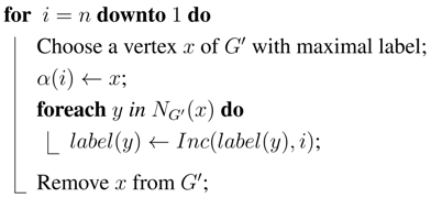
Algorithms MLS and MLSM are given below.

Algorithm MLS (Maximal Label Search)[12]

input   : A graph $G=(V,E)$ and a labeling structure $\mathcal{L}=(L,⪯,l_0,Inc)$.

output   : An ordering α on V, which is a peo of G if G is chordal.

Initialize all labels as l0; $G\prime \leftarrow G$;

Algorithm MLSM (Maximal Label Search for Meo)[12]

input   : A graph $G=(V,E)$ and a labeling structure $\mathcal{L}=(L,⪯,l_0,Inc)$.

output  : An meo α on V and a minimal triangulation $H=G_{\alpha }^{+}$ of G.

Initialize all labels as l0; $E\prime \leftarrow E$; $G\prime \leftarrow G$;

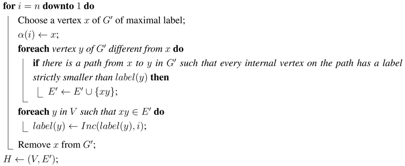When using labeling structure $\mathcal{L}$ with MLS (respectively MLSM), we will refer to the algorithm as $\mathcal{L}$-MLS (respectively $\mathcal{L}$-MLSM). We call any ordering on V that can be produced by MLS (respectively MLSM, $\mathcal{L}$-MLS, $\mathcal{L}$-MLSM) an MLS (respectively MLSM, $\mathcal{L}$-MLS, $\mathcal{L}$-MLSM) ordering.

The following Property was proved in [12]:

Property 3.2 ([12] ) For any graph G and any labeling structure $\mathcal{L}$, Algorithm $\mathcal{L}$-MLSM computing ordering α on G has the same behavior as $\mathcal{L}$-MLS on $G_{\alpha }^{+}$. That is, they give the same labels and numbers to vertices, provided that they break ties in the same way.

Property 3.2 has two important consequences that are used in this paper:

Consequence 1: Any $\mathcal{L}$-MLSM ordering α of G is a $\mathcal{L}$-MLS ordering of $G_{\alpha }^{+}$. Thus a property of MLS on chordal graphs can in some cases be extended to a property of MLSM on arbitrary graphs since $G_{\alpha }^{+}$ is chordal (This is used in Theorem 4.1 and in Property 4.5).

Consequence 2: MLS and MLSM have the same behavior on a chordal graph, since in that case, $G_{\alpha }^{+}=G$. Any execution of MLS on a chordal graph can be seen as an execution of MLSM, and conversely. Thus any property of MLSM on arbitrary graphs also holds for MLS on chordal graphs.

3.2. Specific search algorithms

LexBFS, MCS and MNS are instances of MLS and LEX M, MCS-M and MNSM (defined in [12] from MNS) are instances of MLSM, with the following respective labeling structures:

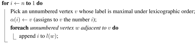
• LexBFS and LEX M: $\mathcal{L}$ is the set of lists of elements of $\{2,3,...,\}$, ⪯ is lexicographical order(a total order), $l_0$ is the empty list, $Inc(l,i)$ is obtained from l by adding i to the end of the list.
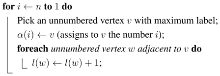
• MCS and MCS-M: $\mathcal{L}=\{0,1,2,...\}$, ⪯ is ≤ (a total order), $l_0=0$, $Inc(l,i)=l+1$.
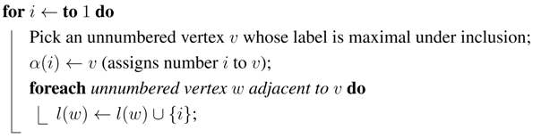
• MNS and MNSM: $\mathcal{L}$ is the power set of $\{2,3,...\}$, ⪯ is ⊆ (not a total order), $l_0=\varnothing$, $Inc(l,i)=l\cup \left\{i\right\}$.

Algorithm LexBFS (Lexicographic Breadth-First Search)[4]

input   : A graph $G=(V,E)$.

output  : An ordering α of V.

Initialize all labels as the empty string;

Algorithm MCS (Maximal Cardinality Search)[5]

input   : A graph $G=(V,E)$.

output  : An ordering α of V.

Initialize all labels as 0;

Algorithm MNS (Maximal Neighborhood Search)[11]

input   : A graph $G=(V,E)$.

output  : An ordering α of V.

Initialize all labels as the empty set;

LEX M and MCS-M can be directly extended from LexBFS and MCS using MLSM.

4. The Separator Structure in the Neighborhood of Vertex 1

In this section, we will study the substars of the vertex numbered 1 by MLS (on a chordal graph) or MLSM (on an arbitrary graph) (i.e., the minimal separators included in the neighborhood of 1).

4.1. Results on the separator structure

Our main result is that if there are several minimal separators $S_1,...S_k$ in this neighborhood, then there is an inclusion order $S_1\subseteq ....\subseteq S_k$ on these separators:

Theorem 4.1

a) 

For any chordal graph H and any MLS ordering α of H, the minimal separators of H included in $N\left(\alpha \right(1\left)\right)$ are totally ordered by inclusion. 

b) 

For any graph G and any MLSM ordering α of G, the minimal separators of G included in $N\left(\alpha \right(1\left)\right)$ are totally ordered by inclusion. 

Example 4.2 In Figure 4, describing an execution of MCS on a chordal graph, the substars of 1 are $\left\{8\right\}$ and $\{3,8\}$; $\left\{8\right\}\subseteq \{3,8\}$.

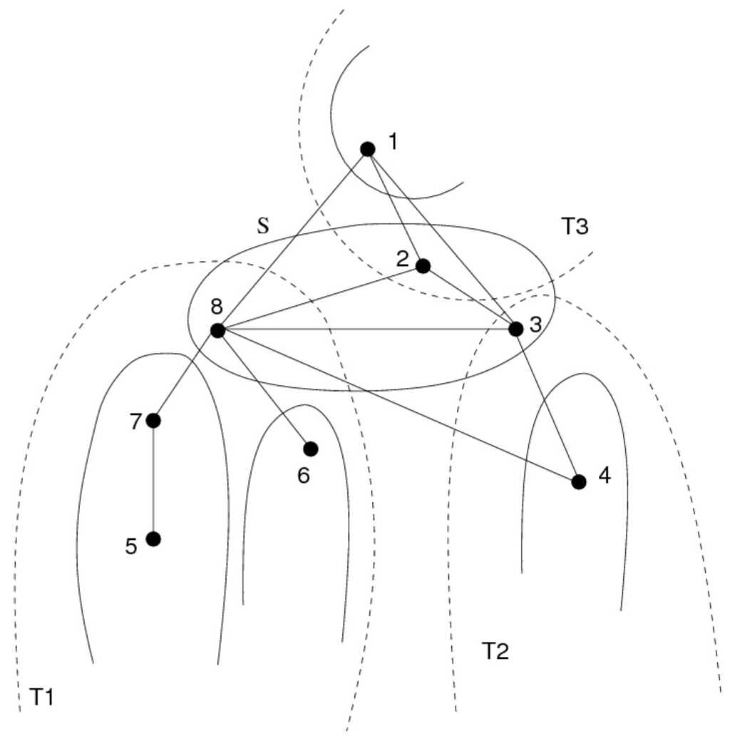
Figure 4. The slices defined by an execution of MCS on a chordal graph. The substars of 1 are $\left\{8\right\}$ and $\{3,8\}$.

In order to prove Theorem 4.1, we need to examine how the search algorithms scan the various connected components defined by these separators. We will need to introduce some notations and definitions in order to describe this.

Let us first explain the structure of the neighborhood of vertex 1, as illustrated by Figure 4.

• The neighborhood of 1 contains minimal separators $A_1,...,A_k$, which are the substars of 1. In our example from Figure 4, $A_1=\left\{8\right\}$ and $A_2=\{3,8\}$.
• The removal of $N\left[1\right]$ defines connected components. In our example, $C_1=\{5,7\}$, $C_1^{\prime }\left\{6\right\}$, $C_2=\left\{4\right\}$.
• The neighborhoods of these components are the substars of 1: $N\left(C_1\right)=N\left(C_1^{\prime }\right)=A_1=\left\{8\right\}$; $N\left(C_2\right)=A_2=\{3,8\}$. Thus with each substar is associated at least one of these components; when there are several components for the same substar, we will need to group them into what we call super-components: $T_1=C_1\cup C_1^{\prime }=\{5,6,7\}$ is a super-component.
• We will see that in some cases, the MLS algorithms will first number all the vertices of the super-component $T_1$ which corresponds to the smallest substar $A_1$ as well as this substar. It will then go on to number the super-component $T_2$ which corresponds to the second smallest substar $A_2$ as well as what is left of this substar, and so forth. This is the case in our example: substar $\left\{8\right\}$ along with super-component $T_1=\{5,6,7\}$ will be numbered first (from 8 to 5), then super-component $T_2=\left\{4\right\}$ will be numbered along with what is left of substar $\{3,8\}$, which is $\left\{3\right\}$, thus numbering from 4 to 3.
  We will call these numbering classes slices.
• The largest substar, $A_k$, defines a connected component which contain vertex 1, as well as the neighbors of 1 which do not belong to any substar (2 in our example). This component ($\{1,2\}$ in our example) defines our slice of largest number, and we will see that it defines a moplex.

We will now give precise notations for these notions:

Notations 4.3 For any graph $G=(V,E)$ and any ordering α on V,

• a component $C_i$ is a connected component of $G(V-N(\alpha \left(1\right)\left)\right)$.
• a super-component $D_i$ is the union of all components with a common neighborhood.
• p denotes the number of super-components 
• $(D_1,D_2,...,D_p)$ denotes the sequence of the super-components ordered as follows: $\forall i\in [1,p-1]$, ${\alpha }^{-1}\left(d_i\right)>{\alpha }^{-1}\left(d_{i+1}\right)$, where $d_i$ denotes the vertex of $D_i$ with maximum number (${\alpha }^{-1}\left(d_i\right)=max\{{\alpha }^{-1}\left(d\right),d\in D_i\}$). 
• the slices are the subsets $T_1$, $T_2$, ..., $T_p$ of V partitioning V as follows: $\forall i\in [1,p]$, $T_i=D_i\cup S_i$, where $S_i=N\left(D_i\right)-\left({\cup }_{1\le j<i}N\left(D_j\right)\right)=N\left(D_i\right)-\left({\cup }_{1\le j<i}{S}_j\right)$, and $t_i$ denotes the vertex of $T_i$ with maximum number. 
  We say that α numbers the slices in increasing order if it numbers the vertices of $T_1$ first (with the largest numbers), then the vertices of $T_2$ etc., i.e., if $\forall i\in [1,p-1]$, $\forall t\in T_i$, ${\alpha }^{-1}\left(t\right)>{\alpha }^{-1}\left(t_{i+1}\right)$. 

Example 4.4 Let us summarize what we can see in Figure 4, which shows the slices defined by an execution of MCS on a chordal graph.

• $N\left(1\right)=\{8,3,2\}$
• Substars: $A_1=\left\{8\right\}$ and $A_2=\{3,8\}$. 
• Components: $C_1=\{5,7\}$, $C_1^{\prime }\left\{6\right\}$, $C_2=\left\{4\right\}$, with $N\left(\right\{7,5\left\}\right)=N\left(\right\{6\left\}\right)=\left\{8\right\}$, $N\left(\right\{4\left\}\right)=\{8,3\}$. 
• Super-components: 
  - $D_1=\{7,5\}\cup \left\{6\right\}=\{7,6,5\}$, $d_1=7$, $S_1=\left\{8\right\}$, $T_1=\{8,7,6,5\}$ and $t_1=8$,
  - $D_2=\left\{4\right\}$, $d_2=4$, $S_2=\left\{3\right\}$, $T_2=\{4,3\}$ and $t_2=4$,
  - $D_3=\left\{1\right\}$, $d_3=1$, $S_3=\left\{2\right\}$, $T_3=\{2,1\}$ and $t_3=2$,
  so $p=3$.
• We observe that: 
  - $N\left(D_1\right)\subset N\left(D_2\right)\subset N\left(D_3\right)$,
  - α numbers the slices in increasing order.

The properties described above can be generalized to the MLS and MLSM orderings, provided that the order on the labels is a total order (such as the one used for LexBFS and MCS):

Property 4.5

(a) 

For any chordal graph H and any labeling structure $\mathcal{L}$, if the order on labels is total then any $\mathcal{L}$-MLS ordering of H numbers the slices in increasing order. 

(b) 

For any graph G and any labeling structure $\mathcal{L}$, if the order on labels is total then any $\mathcal{L}$-MLSM ordering of G numbers the slices in increasing order. 

The following (technical) lemma is the basis for our proofs in this section:

Lemma 4.6 For any MLS ordering α of a chordal graph,

• (a) for any i from 1 to p, $\forall s\in N\left(\alpha \right(1\left)\right)$, if ${\alpha }^{-1}\left(s\right)>{\alpha }^{-1}\left(d_i\right)$ then $s\in N\left(d_i\right)$, 
• (b) for any i from 1 to $p-1$, ${\alpha }^{-1}\left(t_i\right)\ge {\alpha }^{-1}\left(d_i\right)>{\alpha }^{-1}\left(t_{i+1}\right)$, 
• (c) for any i from 1 to $p-1$, $\forall s\in S_i$, ${\alpha }^{-1}\left(s\right)>{\alpha }^{-1}\left(t_{i+1}\right)$, 
• (d) for any i from 1 to $p-1$, if the order on labels is total then $\forall d\in D_i$, ${\alpha }^{-1}\left(d\right)>{\alpha }^{-1}\left(t_{i+1}\right)$. 

We will devote Subsection 4.2. to the proof of this lemma (this subsection can be skipped by the reader not interested in the details of our proofs), then go on to use this lemma to finish our proofs.

4.2. A technical lemma

To prove Lemma 4.6, we will use the following notations and preliminary Lemmas.

Notations 4.7 For any execution of MLS on any graph G computing ordering α and any vertices x and y of G such that ${\alpha }^{-1}\left(x\right)\ge {\alpha }^{-1}\left(y\right)$, 

(i) $l_x\left(y\right)$ denotes the label of y just before numbering x, 

(ii) $N{N}_x\left(y\right)$ denotes the set of Numbered Neighbors of y just before numbering x, i.e., $N{N}_x\left(y\right)=\{z\in N\left(y\right)|{\alpha }^{-1}\left(z\right)>{\alpha }^{-1}\left(x\right)\}$. 

The subscript will be omitted when the considered step is clear from the context. 

The following Lemma is given in [12].

Lemma 4.8 ([12]) At any step of an execution of MLS on a graph G, for any unnumbered vertices $u,v$ of G,

(i) if $NN\left(u\right)=NN\left(v\right)$ then $l\left(u\right)=l\left(v\right)$, 

(ii) if $NN\left(u\right)\subset NN\left(v\right)$ then $l\left(u\right)\prec l\left(v\right)$. 

Lemma 4.9 For any MLS ordering α of a chordal graph, $\forall i\in [1,p]$,

(1) $N{N}_{d_i}\left(d_i\right)=N{N}_{d_i}\left(\alpha \left(1\right)\right)\subseteq N\left(D_i\right)$, 

(2) if $i<p$ then ${\alpha }^{-1}\left(t_i\right)\ge {\alpha }^{-1}\left(d_i\right)>{\alpha }^{-1}\left(t_{i+1}\right)$, 

(3) $N{N}_{t_i}\left(t_i\right)=N{N}_{t_i}\left(\alpha \left(1\right)\right)$. 

Proof: (1) $N{N}_{d_i}\left(d_i\right)\subseteq N{N}_{d_i}\left(\alpha \left(1\right)\right)$ by definition of $d_i$ and $N{N}_{d_i}\left(d_i\right)\not\subset N{N}_{d_i}\left(\alpha \left(1\right)\right)$ (otherwise by Lemma 4.8 $l_{d_i}\left(d_i\right)\prec l_{d_i}\left(\alpha \left(1\right)\right)$, which contradicts the choice of $d_i$ at that step). Hence $N{N}_{d_i}\left(d_i\right)=N{N}_{d_i}\left(\alpha \left(1\right)\right)\subseteq N\left[D_i\right]\cap N\left(\alpha \left(1\right)\right)=N\left(D_i\right)$.

(2) We suppose that $i<p$. By definition of $d_i$ and $t_i$, ${\alpha }^{-1}\left(t_i\right)\ge {\alpha }^{-1}\left(d_i\right)$. Let us show that ${\alpha }^{-1}\left(d_i\right)>{\alpha }^{-1}\left(t_{i+1}\right)$. If $t_{i+1}\notin N\left(\alpha \left(1\right)\right)$ then $t_{i+1}=d_{i+1}$ and we are done since by definition of $d_i$, ${\alpha }^{-1}\left(d_i\right)>{\alpha }^{-1}\left(d_{i+1}\right)$. Otherwise, assume for contradiction that ${\alpha }^{-1}\left(t_{i+1}\right)>{\alpha }^{-1}\left(d_i\right)$. Then $t_{i+1}\in N{N}_{d_i}\left(\alpha \left(1\right)\right)$, and by statement 1 we have: $N{N}_{d_i}\left(\alpha \left(1\right)\right)\subseteq N\left(D_i\right)\subseteq V-T_{i+1}$, so $t_{i+1}\notin T_{i+1}$, a contradiction.

(3) For any $j<i$, $N{N}_{t_i}\left(t_i\right)\cap D_j=\varnothing$ because $N\left(t_i\right)\cap D_j=\varnothing$ (since $T_i\cap N\left(D_j\right)=\varnothing$), and for any $j\ge i$, $N{N}_{t_i}\left(t_i\right)\cap D_j=\varnothing$ because by 2), $\forall t\in T_j$ ${\alpha }^{-1}\left(t_i\right)\ge {\alpha }^{-1}\left(t_j\right)\ge {\alpha }^{-1}\left(t\right)$. It follows that $N{N}_{t_i}\left(t_i\right)\subseteq N{N}_{t_i}\left(\alpha \left(1\right)\right)$, and we show the equality as above for $d_i$.     □

It is easy to show the following lemma:

Lemma 4.10 If G is a chordal graph, μ a chordless path in G and z a vertex of G not belonging to μ and seeing both extremities of μ, then z sees every vertex of μ.

Lemma 4.11 Let G be a chordal graph, let α be an MLS ordering of G, and for $i=1,2,...,p$, let $s\in S_i$ such that ${\alpha }^{-1}\left(d_i\right)>{\alpha }^{-1}\left(s\right)$. Since $s\in S_i$, there exists a chordless path μ from $d_i$ to s such that every internal vertex of μ belongs to $D_i$. Then the following property P holds just after processing $d_i$ and remains true until numbering s.

P : there is a vertex v of μ such that every vertex of $\mu [v,s]$ is unnumbered, $NN\left(\alpha \right(1\left)\right)\subset NN\left(v\right)$ and $\forall t\in \mu [v,s]-\left\{v\right\}$, $NN\left(t\right)=NN\left(\alpha \right(1\left)\right)$. 

Proof: Let us show that P holds just after processing $d_i$. $N{N}_{d_i}\left(d_i\right)=N{N}_{d_i}\left(\alpha \left(1\right)\right)$ by Lemma 4.9, so $N{N}_{d_i}\left(\alpha \left(1\right)\right)\subseteq N\left(d_i\right)$. Also $N{N}_{d_i}\left(\alpha \left(1\right)\right)\subseteq N\left(s\right)$ since, as α is a peo of G, $N\left(\alpha \right(1\left)\right)$ is a clique of G. It follows by Lemma 4.10 that for any vertex t of μ, $N{N}_{d_i}\left(\alpha \left(1\right)\right)\subseteq N\left(t\right)$, so $N{N}_{d_i}\left(\alpha \left(1\right)\right)\subseteq N{N}_{d_i}\left(t\right)$, and as the reverse inclusion holds by definition of $d_i$ and $S_i$, $N{N}_{d_i}\left(t\right)=N{N}_{d_i}\left(\alpha \left(1\right)\right)$. After processing $d_i$, $NN\left(\alpha \right(1\left)\right)$ is unchanged and P is true, taking as vertex v the vertex of μ next to $d_i$ (which is the only vertex of μ seeing $d_i$ since μ is chordless).

Let us show that P is true after processing some vertex w, ${\alpha }^{-1}\left(d_i\right)>{\alpha }^{-1}\left(w\right)>{\alpha }^{-1}\left(s\right)$.

First case: $w\notin N\left(\alpha \right(1\left)\right)$.

If no vertex of $\mu [v,s]$ sees w then $w\notin \mu [v,s]$ and P remains true with the same vertex v, otherwise P remains true, taking as new vertex v the last vertex of $\mu [v,s]$ seeing w.

Second case: $w\in N\left(\alpha \right(1\left)\right)$.

$ws$ is an edge of G, as $N\left(\alpha \right(1\left)\right)$ is a clique. We get from edge $ws$ and path $\mu [v,s]$ a $wv$-path such that every internal vertex t is unnumbered and satisfies $NN\left(t\right)=NN\left(\alpha \right(1\left)\right)\subset NN\left(v\right)$, so by Lemma 4.8 $l\left(t\right)\prec l\left(v\right)$. By Property 3.2, this execution of MLS on chordal graph G can be seen as an execution of MLSM, according to which $wv$ will be an edge of H with $H=G_{\alpha }^{+}=G$. It follows that w sees v in G. By Lemma 4.10 w sees every vertex of $\mu [v,s]$. It follows that when processing w, w is added to $NN\left(\alpha \right(1\left)\right)$ as well as to $NN\left(t\right)$ for every vertex t of $\mu [v,s]$, and P remains true with the same vertex v.     □

Lemma 4.12 For any MLS ordering α of a chordal graph, $\forall i\in [1,p-1],\forall s\in S_i$, ${\alpha }^{-1}\left(s\right)>{\alpha }^{-1}\left(t_{i+1}\right)$.

Proof: Suppose there is some $s\in S_i$ such that ${\alpha }^{-1}\left(t_{i+1}\right)>{\alpha }^{-1}\left(s\right)$. Then by Lemma 4.9 ${\alpha }^{-1}\left(d_i\right)>{\alpha }^{-1}\left(t_{i+1}\right)>{\alpha }^{-1}\left(s\right)$. Lemma 4.11 ensures the existence of some vertex v such that $N{N}_{t_{i+1}}\left(\alpha \left(1\right)\right)\subset N{N}_{t_{i+1}}\left(v\right)$, so by Lemma 4.9 $N{N}_{t_{i+1}}\left(t_{i+1}\right)\subset N{N}_{t_{i+1}}\left(v\right)$ and by Lemma 4.8 $l_{t_{i+1}}\left(t_{i+1}\right)\prec l_{t_{i+1}}\left(v\right)$, which contradicts the choice of $t_{i+1}$ at that step.     □

Lemma 4.13 For any MLS ordering α of a chordal graph, if the order on labels is total then $\forall i\in [1,p-1]$, $\forall d\in D_i$, ${\alpha }^{-1}\left(d\right)>{\alpha }^{-1}\left(t_{i+1}\right)$.

Proof: Suppose there is some $d\in D_i$ such that ${\alpha }^{-1}\left(t_{i+1}\right)>{\alpha }^{-1}\left(d\right)$. We can choose d as the first vertex of $D_i$ numbered after $t_{i+1}$. Just before numbering $t_{i+1}$, $l\left(t_{i+1}\right)$ is maximum (since the order ⪯ is total) with $l_{t_{i+1}}\left(t_{i+1}\right)=l_{t_{i+1}}\left(\alpha \left(1\right)\right)$ by Lemmas 4.9 and 4.8, so $l_{t_{i+1}}\left(d\right)⪯l_{t_{i+1}}\left(\alpha \left(1\right)\right)$. As by Lemma 4.12, every vertex of $N\left(D_i\right)$ is numbered before $t_{i+1}$, $l\left(d\right)$ remains equal to $l_{t_{i+1}}\left(d\right)$ until d is numbered. We thus only have to prove that $l\left(\alpha \right(1\left)\right)$ is incremented before numbering d. This will lead to a contradiction, since $\alpha \left(1\right)$ is numbered last.

If $t_{i+1}\in N\left(\alpha \left(1\right)\right)$, $l\left(\alpha \right(1\left)\right)$ is incremented when numbering $t_{i+1}$ and we are done.

If $t_{i+1}\notin N\left(\alpha \left(1\right)\right)$, $t_{i+1}=d_{i+1}$. By Property 4.14, $S_{i+1}$ is not empty, so let $s\in S_{i+1}$. ${\alpha }^{-1}\left(d_{i+1}\right)>{\alpha }^{-1}\left(s\right)$, and by Lemma 4.11, until numbering s, there is some unnumbered vertex v such that $NN\left(\alpha \right(1\left)\right)\subset NN\left(v\right)$, so by Lemma 4.8 $l\left(\alpha \right(1\left)\right)\prec l\left(v\right)$, hence $l\left(d\right)\prec l\left(v\right)$. This implies that ${\alpha }^{-1}\left(s\right)>{\alpha }^{-1}\left(d\right)$ and as $l\left(\alpha \right(1\left)\right)$ is incremented when processing s, it is incremented before numbering d.     □

As Lemma 4.6 a) can be rewritten as $N{N}_{d_i}\left(\alpha \left(1\right)\right)\subseteq N{N}_{d_i}\left(d_i\right)$, Lemma 4.6 directly follows from Lemmas 4.9, 4.12 and 4.13.

4.3. Proofs of Theorem 4.1 and Property 4.5

Property 4.14 For any chordal graph G and any MLS ordering α of G, for any super-component $D_i$, $i\in \{1,2...p\}$, $N\left(D_i\right)\subset N\left(D_{i+1}\right)$.

Proof: Let $s\in N\left(D_i\right)$, and let $j\le i$ such that $s\in S_j$. By Lemma 4.6 (b) and (c), ${\alpha }^{-1}\left(s\right)>{\alpha }^{-1}\left(t_{j+1}\right)\ge {\alpha }^{-1}\left(t_{i+1}\right)\ge {\alpha }^{-1}\left(d_{i+1}\right)$, so by Lemma 4.6 a) $s\in N\left(D_{i+1}\right)$. Thus $N\left(D_i\right)\subseteq N\left(D_{i+1}\right)$ and, as $N\left(D_i\right)\ne N\left(D_{i+1}\right)$ by definition of the sequence $\left(D_i\right)$, $N\left(D_i\right)\subset N\left(D_{i+1}\right)$. □□□□

For any graph G and any ordering α on V, the minimal separators of G included in $N\left(\alpha \right(1\left)\right)$ are exactly the neighborhoods of the components different from $\left\{\alpha \right(1\left)\right\}$ [18], which are also the neighborhoods of the super-components of $(G,\alpha )$ different from $\left\{\alpha \right(1\left)\right\}$. Therefore, Theorem 4.1(a) follows from Property 4.14. Property 4.5(a) follows immediately from Lemma 4.6 (c) and (d).

By Property 3.2 any $\mathcal{L}$-MLSM ordering α of any graph G is a $\mathcal{L}$-MLS ordering of $G_{\alpha }^{+}$, which verifies the above neighborhood properties since $G_{\alpha }^{+}$ is chordal. Moreover, the neighborhood of $\alpha \left(1\right)$ is the same in G as in $G_{\alpha }^{+}$ (by definition of $G_{\alpha }^{+}$) and since α is a meo of G, the components of $(G,\alpha )$ and of $(G_{\alpha }^{+},\alpha )$ are the same with the same neighborhoods. (This follows from Theorem 5.12, Invariant 4.9 and Lemma 6.2 in [19]). Thus the super-components, their neighborhoods and the slices of $(G,\alpha )$ and of $(G_{\alpha }^{+},\alpha )$ are the same, and Theorem 4.1(a) and Property 4.5(a) extend to MLSM on an arbitrary graph, yielding Theorem 4.1(b) and Property 4.5(b).

If the order on the labels is not total, an $\mathcal{L}$-MLSM ordering (or an $\mathcal{L}$-MLS ordering on a chordal graph) does not necessarily number the slices in increasing order. Figure 5 gives a counterexample demonstrating this.

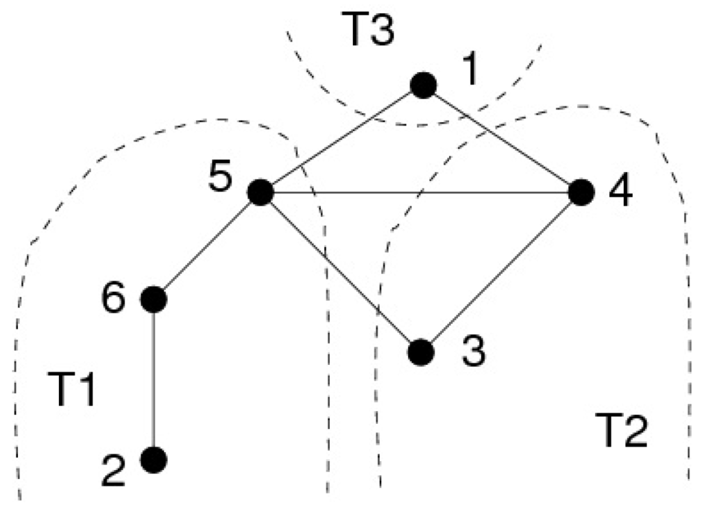
Figure 5. This MNS ordering does not number slices in increasing order on this chordal graph. (The MNS labels are sets of numbers of neighbors, and set comparison by ⊆ is not a total order.)

4.4. The separator structure of MLS on a non-chordal graph

Though the algorithms of the MLS family were meant to be run on a chordal graph (in order to compute a peo), we investigated MLS run on a non-chordal graph. The results are negative: on a non-chordal graph MLS does not, in general, exhibit properties such as those described above, even when the order ⪯ is total. Figure 6 gives a counter-example of this, using MCS as an instantiation of MLS. The substars of 1 are $\{2,6\}$ and $\{3,6\}$, which are not inclusive. The components of $G(V-N[1\left]\right)$ are not numbered following any particular order.

However, we will see in Section 5 that MLS run on a non-chordal graph with a total order on the labels always ends on an OCF-vertex of the graph.

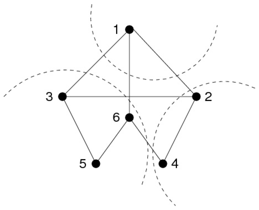
Figure 6. MCS on a non-chordal graph. Substars of 1: $\{2,6\}$ and $\{3,6\}$. These substars are not pairwise inclusive.

5. The Extremities Defined by MLS and MLSM

5.1. The extremal moplexes defined by MLS and MLSM

For any MLSM ordering α of a graph G, since α is a meo of G, by [15]$\alpha \left(1\right)$ is an OCF-vertex of G. We will show a stronger property: $\alpha \left(1\right)$ is a vertex of a moplex.

Theorem 5.1

• For any chordal graph H and any labeling structure $\mathcal{L}$, $\mathcal{L}$-MLS ends on a vertex belonging to a moplex. If moreover the order on the labels is total, then the vertices of this moplex are numbered consecutively. 
• For any graph G and any labeling structure $\mathcal{L}$, $\mathcal{L}$-MLSM ends on a vertex belonging to a moplex. If moreover the order on labels is total, then the vertices of this moplex are numbered consecutively. 

To prove this, we need only use the properties of the neighborhood of $\alpha \left(1\right)$ described in Section 4 and the following Lemma.

Lemma 5.2 For any graph G and any vertex x of G, x is a vertex of a moplex if and only if x is an OCF-vertex and the set of minimal separators of G included in $N\left(x\right)$ has a greatest element $S_{max}$ with respect to inclusion. In that case, the moplex containing x is $N\left[x\right]-S_{max}$.

Proof: We suppose that x is a vertex of a moplex X of G. Then $N\left[x\right]=N\left[X\right]$ and there is a connected component C of $G(V-N[x\left]\right)$ such that $N\left(C\right)=N\left(X\right)$. Since X is a clique module of G, any non-adjacent neighbors of x must belong to $N\left(X\right)$; i.e. to $N\left(C\right)$, so x is an OCF-vertex of G, and the neighborhood of any connected component of $G(V-N[x\left]\right)$ is a subset of $N\left(X\right)$ i.e. of $N\left(C\right)$, so $N\left(C\right)$ is the greatest minimal separator of G included in $N\left(x\right)$ with respect to inclusion.

Conversely, we suppose that x is an OCF-vertex of G and the set of minimal separators of G included in $N\left(x\right)$ has a greatest element $S_{max}$ with respect to inclusion. Let $X=N\left[x\right]-S_{max}$. We immediately verify that X is a clique module of G, with $N\left(X\right)=S_{max}$. Let C be the connected component of $G(V-N[x\left]\right)$ such that $S_{max}=N\left(C\right)$. X and C are distinct connected components of $G(V-N(X\left)\right)$ such that $N\left(X\right)=N\left(C\right)$, so $N\left(X\right)$ is a minimal separator of G and therefore X is a moplex of G.     □

Proof: (of Theorem 5.1) Since α is a meo of G, $\alpha \left(1\right)$ is an OCF-vertex of G [15]. Moreover, by Theorem 4.1, the set of minimal separators of G included in $N\left(\alpha \right(1\left)\right)$ has a greatest element $S_{max}$ with respect to inclusion. If $D_p=\left\{\alpha \left(1\right)\right\}$ then $S_{max}=N\left(\alpha \left(1\right)\right)$, else $S_{max}=N\left(D_{p-1}\right)$. (Note that $p>1$ because otherwise G would be reduced to the closed neighborhood of OCF-vertex $\alpha \left(1\right)$ and would be a clique). It follows by Lemma 5.2 that $\alpha \left(1\right)$ is a vertex of a moplex X of G, with $X=N\left[\alpha \left(1\right)\right]-S_{max}$. So X is equal to either $\left\{\alpha \right(1\left)\right\}$ or to $D_p$. Thus if the order on labels is total then by Property 4.5 $\mathcal{L}$-MLSM ends on X.

Since by Property 3.2, any chordal graph has the same $\mathcal{L}$-MLS and $\mathcal{L}$-MLSM orderings, we complete our proof for chordal graphs.     □

5.2. MLS on a non-chordal graph

On a non-chordal graph, in general, an MLS execution does not end on a moplex and does not even end on a vertex of a moplex, even if the order on labels is total, as shown by Figure 6 for MCS. However, we show that if the order on labels is total then MLS does ends on an OCF-vertex.

Theorem 5.3 For any graph G, any labeling structure $\mathcal{L}$ and any $\mathcal{L}$-MLS ordering α of G, if the order on labels is total then $\alpha \left(1\right)$ is an OCF-vertex of G.

The proof of Theorem 5.3 uses the following Lemma, where for any vertices x and y of G such that ${\alpha }^{-1}\left(x\right)\ge {\alpha }^{-1}\left(y\right)$, $l_x\left(y\right)$ denotes the label of y just before numbering x.

Lemma 5.4 We consider an MLS execution on a graph G computing α and vertices $u,v$ of G such that ${\alpha }^{-1}\left(u\right)>{\alpha }^{-1}\left(v\right)$. If $l_u\left(v\right)⪯l_u\left(\alpha \left(1\right)\right)$ and every neighbor t of v such that ${\alpha }^{-1}\left(u\right)\ge {\alpha }^{-1}\left(t\right)>{\alpha }^{-1}\left(v\right)$ is a neighbor of $\alpha \left(1\right)$ then $l_v\left(v\right)=l_v\left(\alpha \left(1\right)\right)$ and every neighbor t of $\alpha \left(1\right)$ such that ${\alpha }^{-1}\left(u\right)\ge {\alpha }^{-1}\left(t\right)>{\alpha }^{-1}\left(v\right)$ is a neighbor of v.

Proof: At every step between numbering u and numbering v, if the label of v is incremented then the label of $\alpha \left(1\right)$ is incremented too, so by Properties (p1) and (p2) of Definition 3.1 the inequality $l\left(v\right)⪯l\left(\alpha \right(1\left)\right)$ is preserved, and since $l\left(v\right)$ is maximal just before numbering v, $l_v\left(v\right)=l_v\left(\alpha \left(1\right)\right)$. Now if some vertex t numbered between u and v was a neighbor of $\alpha \left(1\right)$ but not of v then the inequality would become $l\left(v\right)\prec l\left(\alpha \right(1\left)\right)$, which would be preserved until numbering v, a contradiction.     □

Proof: (of Theorem 5.3) We define the partition of V into subsets $T_i^{\prime }$, $1\le i\le p^{\prime }$, which is a variant of the partition of V into thin slices. For any i in $[1,p^{\prime }]$,

- $t_i^{\prime }=\alpha \left(n\right)$ if $i=1$, otherwise $t_i^{\prime }$ is the first vertex numbered after $c_{i-1}^{\prime }$ not belonging to $N\left[C_{i-1}^{\prime }\right]$,

- $c_i^{\prime }=t_i^{\prime }$ if $t_i^{\prime }\notin N\left(\alpha \left(1\right)\right)$, otherwise $c_i^{\prime }$ is the first vertex numbered after $t_i^{\prime }$ which does not belong to $N\left(\alpha \right(1\left)\right)$ ($c_{p^{\prime }}^{\prime }=\alpha \left(1\right)$),

- $C_i^{\prime }$ is the component of $(G,\alpha )$ containing $c_i^{\prime }$ ($C_{p^{\prime }}^{\prime }=\left\{\alpha \left(1\right)\right\}$),

- $T_i^{\prime }$ is the set of vertices t such that ${\alpha }^{-1}\left(t_i^{\prime }\right)\ge {\alpha }^{-1}\left(t\right)$ and (if $i<p^{\prime }$) ${\alpha }^{-1}\left(t\right)>{\alpha }^{-1}\left(t_{i+1}^{\prime }\right)$, so by definition, the subsets $T_i^{\prime }$ are numbered in increasing order.

Note that for any i in $[1,p^{\prime }]$$T_i^{\prime }\subseteq N\left(\alpha \left(1\right)\right)\cup C_i^{\prime }$ and that there may be distinct i, j such that $C_i^{\prime }=C_j^{\prime }$, so $p^{\prime }$ can be greater than the number of components of $(G,\alpha )$.

We first show that for any i in $[1,p^{\prime }]$, $l\left(\alpha \right(1\left)\right)$ is maximum among labels of unnumbered vertices just before numbering $t_i^{\prime }$. The proof goes by induction on i. It obviously holds for $i=1$. We suppose that it holds for some $i<p^{\prime }$. $l_{t_i^{\prime }}\left(t_{i+1}^{\prime }\right)⪯l_{t_i^{\prime }}\left(\alpha \left(1\right)\right)$, and every neighbor t of $t_{i+1}^{\prime }$ in $T_i^{\prime }$ is a neighbor of $\alpha \left(1\right)$ since by definition of $t_{i+1}^{\prime }$, t cannot be in $C_i^{\prime }$. By Lemma 5.4 with $u=t_i^{\prime }$ and $v=t_{i+1}^{\prime }$$l_{t_{i+1}^{\prime }}\left(t_{i+1}^{\prime }\right)=l_{t_{i+1}^{\prime }}\left(\alpha \left(1\right)\right)$, and since $l\left(t_{i+1}^{\prime }\right)$ is maximum at that step (because the order ⪯ is total) $l\left(\alpha \right(1\left)\right)$ is maximum too.

Now let $y,z\in N\left(\alpha \right(1\left)\right)$ such that ${\alpha }^{-1}\left(y\right)>{\alpha }^{-1}\left(z\right)$. Let us show that either $y\in N\left(z\right)$ or there is some $j<p^{\prime }$ such that $y,z\in N\left(C_j^{\prime }\right)$. Let $i\in [1,p^{\prime }]$ such that $y\in T_i^{\prime }$.

First case: $\exists j\in [i,p^{\prime }-1]|z\in N\left(C_j^{\prime }\right)$

Let j be the smallest integer $j^{\prime }$ such that $j^{\prime }\in [i,p^{\prime }-1]$ and $z\in N\left(C_{j^{\prime }}^{\prime }\right)$. If ${\alpha }^{-1}\left(c_j^{\prime }\right)\ge {\alpha }^{-1}\left(y\right)$ then ${\alpha }^{-1}\left(c_j^{\prime }\right)\ge {\alpha }^{-1}\left(y\right)>{\alpha }^{-1}\left(t_{i+1}^{\prime }\right)\ge {\alpha }^{-1}\left(t_{j+1}^{\prime }\right)$, so by definition of $t_{j+1}^{\prime }$ as the first vertex numbered after $c_j^{\prime }$ not belonging to $N\left[C_j^{\prime }\right]$, $y\in N\left(C_j^{\prime }\right)$. Otherwise ${\alpha }^{-1}\left(t_i^{\prime }\right)\ge {\alpha }^{-1}\left(y\right)>{\alpha }^{-1}\left(c_j^{\prime }\right)$ and by Lemma 5.4 with $u=t_i^{\prime }$ and $v=c_j^{\prime }$, $y\in N\left(c_j^{\prime }\right)$, so $y\in N\left(C_j^{\prime }\right)$. Thus in both cases $y,z\in N\left(C_j^{\prime }\right)$.

Second case: $\forall j\in [i,p^{\prime }-1]$, $z\notin N\left(C_j^{\prime }\right)$

${\alpha }^{-1}\left(t_i^{\prime }\right)\ge {\alpha }^{-1}\left(y\right)>{\alpha }^{-1}\left(z\right)$ so by Lemma 5.4 with $u=t_i^{\prime }$ and $v=z$, $y\in N\left(z\right)$.

Hence $\alpha \left(1\right)$ is an OCF-vertex of the input graph.     □

This is the case in particular for MCS (as shown in [16]).

If the order on labels is not total then MLS does not necessarily end on an OCF-vertex. For instance, let G and α be the graph and the ordering shown in Figure 7. Note that α is an MNS ordering of G and $\alpha \left(1\right)$ is not an OCF-vertex of G.

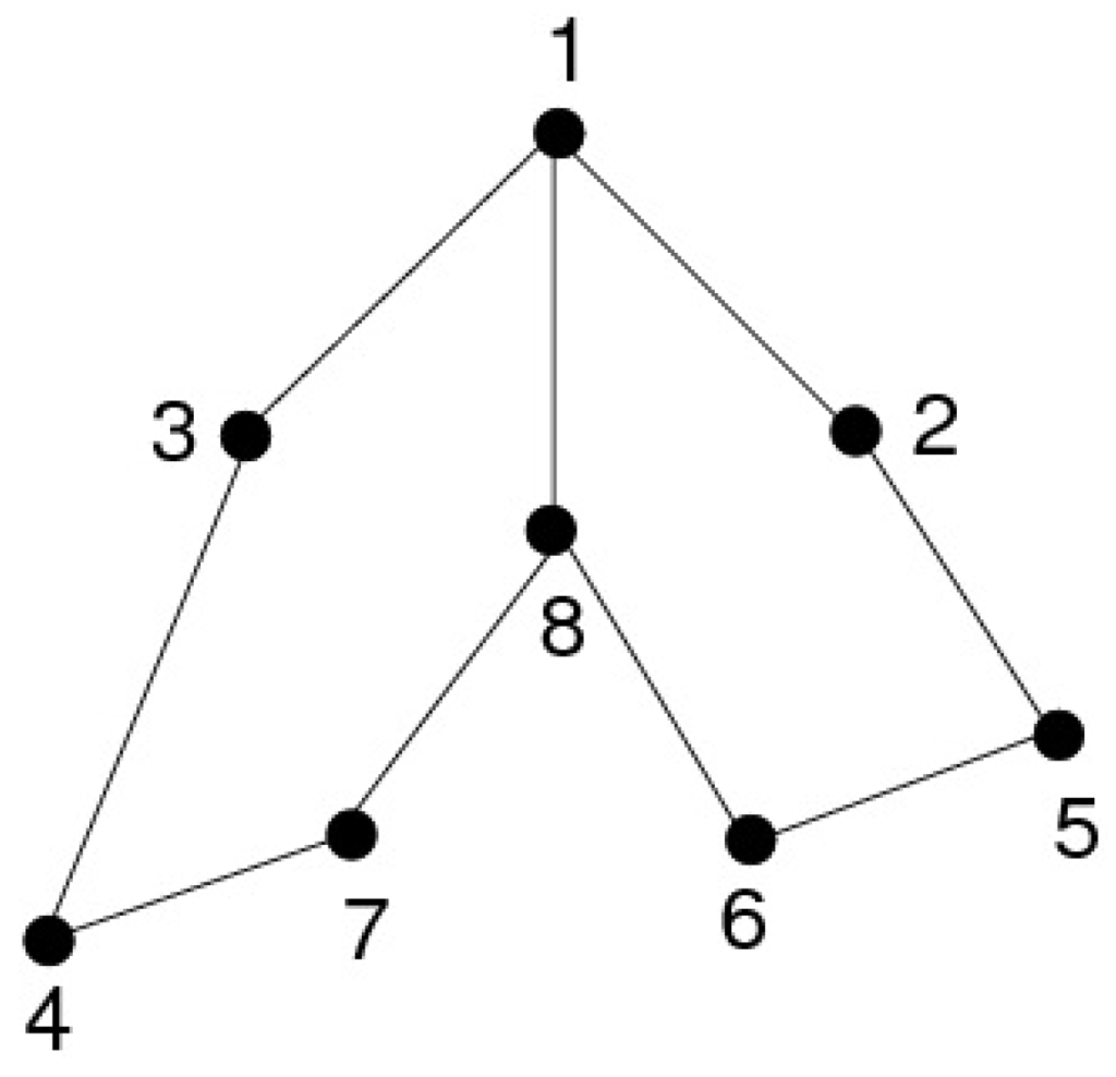
Figure 7. MNS on a non-chordal graph does not end on an OCF-vertex: the substars of 1 are $\{3,8\}$ and $\{2,8\}$, but there is no edge 23.

6. LexBFS, a Special Case

Algorithm LexBFS, with respect to the properties discussed so far, exhibits stronger properties than any other algorithm of the MLS family (as far as we know). In fact, LexBFS, run on a non-chordal graph, has the properties which are those of MLS (with a total order) run on a chordal graph:

• Vertex $\alpha \left(1\right)$ belongs to a moplex, and the vertices of this moplex have consecutive numbers.
• The minimal separators included in the neighborhood of vertex 1 are totally ordered by inclusion.

Moreover, LexBFS refines the numbering of the slices: LexBFS numbers the components of $G(V-N(\alpha \left(1\right))$ one by one, instead of numbering the slices (which are groups of components) one by one. As we will see, we will thus partition the slices into thin slices.

The following result is shown in [13] see their Theorem 5.1 and their Property 5.5):

Theorem 6.1 [13] In an arbitrary graph, the vertex numbered 1 by LexBFS belongs to a moplex whose vertices are numbered consecutively.

Example 6.2 Figure 8 shows an execution of LexBFS on a non-chordal graph G. The moplex containing $\alpha \left(1\right)$ is $X_1=\{1,2\}$.

Let us now consider an execution of LexBFS on an arbitrary graph G, let $X_1$ be the moplex containing vertex $\alpha \left(1\right)$. We will define the thin slices of the execution in a similar fashion to the slices (see Notations 4.3):

Notations 6.3 For any graph $G=(V,E)$ and any LexBFS ordering α on V, with $X_1$ the moplex containing vertex $\alpha \left(1\right)$,

• a component $C_i$ is a connected component of $G(V-N\left(X_1\right))$, with k the number of such components.
• $(C_1,C_2,...,C_k)$ denotes the sequence of the components ordered as follows: $\forall i\in [1,k-1]$, ${\alpha }^{-1}\left(y_i\right)>{\alpha }^{-1}\left(y_{i+1}\right)$, where $y_i$ denotes the vertex of $C_i$ with maximum number (${\alpha }^{-1}\left(y_i\right)=max\{{\alpha }^{-1}\left(y\right),y\in C_i\}$). 
• the thin slices are the subsets $F_1$, $F_2$, ..., $F_k$ of V partitioning V as follows: $\forall i\in [1,k]$, $F_i=C_i\cup S_i$, where $S_i=N\left(C_i\right)-\left({\cup }_{1\le j<i}N\left(C_j\right)\right)=N\left(C_i\right)-\left({\cup }_{1\le j<i}{S}_j\right)$, and $t_i$ denotes the vertex of $F_i$ with maximum number. 
  We say that α numbers the thin slices in increasing order if it numbers the vertices of $F_1$ first (with the largest numbers), then the vertices of $F_2$ etc., i.e. if $\forall i\in [1,k-1]$, $\forall t\in F_i$, ${\alpha }^{-1}\left(t\right)>{\alpha }^{-1}\left(t_{i+1}\right)$. 

Example 6.4 Figure 9 shows the thin slices defined by the LexBFS execution on a non-chordal graph from Figure 8. The thin slices are: $\{10,9,8,7\},\left\{6\right\},\{5,4,3\}$ and $\{2,1\}=X_1$.

We will use the following two lemmas from [13]:

Lemma 6.5 No vertex of $V-C_1\cup N\left(C_1\right)$ can be numbered before all the vertices of $C_1\cup N\left(C_1\right)$ are numbered.

Lemma 6.6 When LexBFS starts numbering $V-(C_1\cup N\left(C_1\right))$, every unnumbered vertex has exactly the same label.

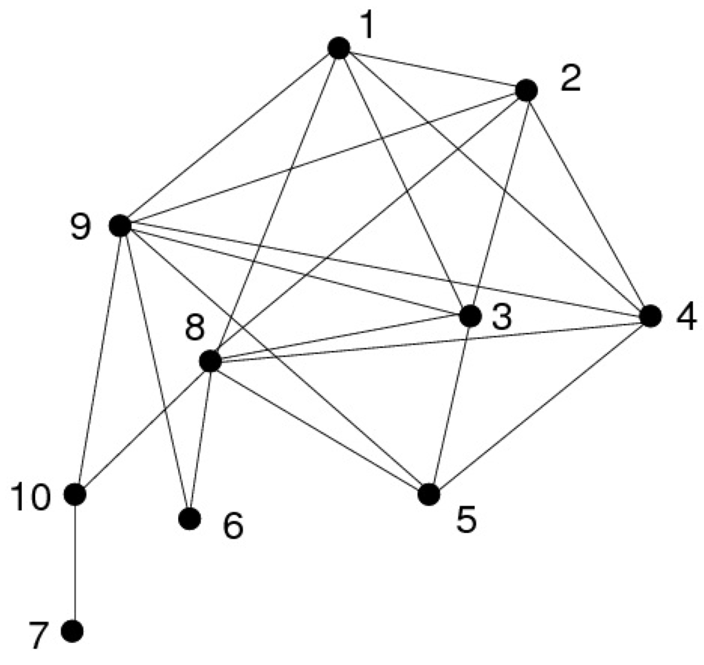
Figure 8. A LexBFS execution on a non-chordal graph. Moplex containing $\alpha \left(1\right)$: $X_1=\{1,2\}$. Components of $G(V-X_1\cup N\left(X_1\right))$: $C_1=\{10,7\}$, $C_2=\left\{6\right\}$, $C_3=\left\{5\right\}$. $N\left(C_1\right)=N\left(C_2\right)=\{9,8\}$, $N\left(C_3\right)=\{9,8,4,3\}$.

From Lemma 6.6, we deduce that the restriction of the LexBFS numbering to $V-C_1\cup N\left(C_1\right)$ will also be a LexBFS numbering of the corresponding subgraph. LexBFS will thus number recursively first $V-C_1\cup N\left(C_1\right)$, then $(C_2\cup N\left(C_2\right))-(C_1\cup N\left(C_1\right))$, and so forth. Thus lemmas 6.5 and 6.6 can easily be extended to the following, where $i>1$:

Lemma 6.7 No vertex of thin slice $F_i$ can be numbered before all the vertices of thin slice $F_{i-1}$ are numbered.

Lemma 6.8 When LexBFS starts numbering thin slice $F_i$, every unnumbered vertex has exactly the same label.

The following property can then be deduced from Lemma 6.7:

Property 6.9 ([13]) For any graph G (chordal or not), any LexBFS ordering α of G numbers the thin slices in increasing order.

We will now prove the separator inclusion:

Theorem 6.10 For any graph G (chordal or not) and any LexBFS ordering α of G, the minimal separators of G included in $N\left(\alpha \right(1\left)\right)$ are totally ordered by inclusion.

Proof: Let $C_1,C_2,...,C_k$ be as above the connected components of $G(V-X_1\cup N\left(X_1\right)$ (where $X_1$ is the moplex containing vertex $\alpha \left(1\right)$). We claim that $N\left(C_1\right)\subseteq N\left(C_2\right)\subseteq ...\subseteq N\left(C_k\right)$. Suppose by contradiction that there are two components $C_i$ and $C_j$, $i<j$, such that $N\left(C_i\right)⊈N\left(C_j\right)$, and let y be in $N\left(C_i\right)-N\left(C_j\right)$. By Lemma 6.8, when LexBFS finishes numbering $C_i\cup N\left(C_i\right))$, all the unnumbered vertices have the same label; since y sees all the vertices of $X_1$, y must also see all the unnumbered vertices of $C_j$, else the labels of $\alpha \left(1\right)$ and of some vertex of $C_j$ would be different. Thus $y\in N\left(C_j\right)$, a contradiction.     □

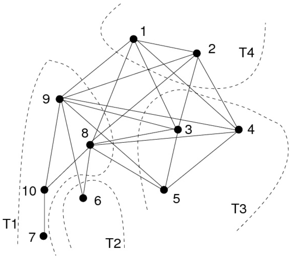
Figure 9. The thin slices defined by the LexBFS execution on a non-chordal graph from Figure 8.

Example 6.11 In Figure 8, the minimal separators included in $N\left(X_1\right)$ are $\{9,8\}$ and $\{9,8,4,3\}$, with $\{9,8\}\subset \{9,8,4,3\}$.

The properties discussed in this section show that LexBFS, when run on a non-chordal graph, exhibits properties which other known algorithms of the MLS family exhibit only on chordal graphs. This may make LexBFS very interesting for specific applications.

7. The Orderings Defined by MLS and MLSM

As explained above, MLS computes a peo of any chordal graph, and MLSM computes a meo of any graph.

We can strengthen these properties to moplex orderings, introduced by [17].

We define a moplex to be simplicial if all its vertices are simplicial. We define a simplicial moplex elimination scheme in a chordal graph by repeatedly choosing a moplex of the current graph, which is simplicial since the graph is chordal, and removing it, until the graph is a clique.

If the graph is not chordal, we define the moplex elimination game in the same way as the simplicial elimination game: we simulate a moplex elimination scheme by repeatedly choosing a moplex of the current graph, adding every edge whose absence violates the simpliciality of this moplex, and removing it, until the graph is a clique.

Thus we obtain an ordered partition $(X_1,X_2,...,X_k)$ where $X_i$ is a moplex of the current graph at step i if $i<k$ and $X_k$ is the final clique. A moplex ordering is an ordering α on V that numbers (from 1 to n) the sets $X_i$ of such an ordered partition in increasing order, i.e. such that $\forall i\in [1,k-1]$, $\forall x\in X_i$, $\forall x^{\prime }\in X_{i+1}$, ${\alpha }^{-1}\left(x\right)<{\alpha }^{-1}\left(x^{\prime }\right)$. Then $G_{\alpha }^{+}$ is exactly the graph obtained from G by adding all edges added in the moplex elimination game.

Any LexBFS ordering of a chordal graph, and any LEX M ordering of any graph, defines a moplex ordering [17]. We extend these results to MLS and MLSM:

Theorem 7.1

(a) 

For any chordal graph H and any labeling structure $\mathcal{L}$, if the order on labels is total, then any $\mathcal{L}$-MLS ordering of H defines a moplex ordering. 

(b) 

For any graph G and any labeling structure $\mathcal{L}$, if the order on labels is total, then any $\mathcal{L}$-MLSM ordering of G defines a moplex ordering. 

Proof: For any chordal graph G and any labeling structure $\mathcal{L}$, if the order on labels is total then any $\mathcal{L}$-MLS ordering of G is a moplex ordering of G: we have only to point out that by Theorem 5.1, any $\mathcal{L}$-MLS ordering α of a non-clique chordal graph G ends on a moplex X of G and that the restriction of α to the chordal subgraph $G(V-X)$ is itself a $\mathcal{L}$-MLS ordering of this subgraph, and the proof follows by induction on $\left|V\right|$.

For any graph G and any labeling structure $\mathcal{L}$, if the order on labels is total then any $\mathcal{L}$-MLSM ordering of G is a moplex ordering of G: let α be a $\mathcal{L}$-MLSM ordering of G. For any k from 1 to n, let $G_{\alpha }^k$ denote the current graph of the simplicial elimination game just before processing $\alpha \left(k\right)$, let $V_{\alpha }^k$ be its set of vertices, i.e. $V_{\alpha }^k=\{\alpha \left(k\right),...,\alpha \left(n\right)\}$, and ${\alpha }_k$ be the restriction of α to $V_{\alpha }^k$. To prove that α is a moplex ordering of G, it is sufficient to prove that for any k from 1 to n such that $G_{\alpha }^k$ is not a clique, ${\alpha }_k$ ends on a moplex of $G_{\alpha }^k$. Consider any k, $1\le k\le n$, such that $G_{\alpha }^k$ is not a clique and let us show that ${\alpha }_k$ ends on a moplex of $G_{\alpha }^k$.

By Property 3.2 α is a $\mathcal{L}$-MLS ordering of $G_{\alpha }^{+}$, so ${\alpha }_k$ is a $\mathcal{L}$-MLS ordering of $G_{\alpha }^{+}\left(V_{\alpha }^k\right)$, which is equal to ${\left(G_{\alpha }^k\right)}_{{\alpha }_k}^{+}$. As α is a meo of G, its restriction ${\alpha }_k$ is a meo of $G_{\alpha }^k$, for otherwise there would exist another ordering ${\beta }_k$ on $V_{\alpha }^k$ that produces some better fill-in than ${\alpha }_k$, and therefore an ordering β on V that produces some better fill-in than α, a contradiction. So, ${\left(G_{\alpha }^k\right)}_{{\alpha }_k}^{+}$ is a minimal triangulation of $G_{\alpha }^k$ and therefore, as $G_{\alpha }^k$ is not a clique, ${\left(G_{\alpha }^k\right)}_{{\alpha }_k}^{+}$ is not a clique either. It follows from Theorem 5.1 that ${\alpha }_k$ ends on a moplex of ${\left(G_{\alpha }^k\right)}_{{\alpha }_k}^{+}$, which is also a moplex of $G_{\alpha }^k$ since any moplex of a minimal triangulation of a graph is a moplex of this graph [13].     □

8. The MLS-Terminal Vertex Problem on Chordal Graphs

To conclude our investigation of the extremities defined by the MLS family of algorithms, we will ask the following question:

“Given a graph G and a vertex x of G, is there an MLS execution which gives number 1 to vertex x ?”

We call this the MLS-Terminal Vertex Problem.

Lanlignel [20] showed that LexBFS-Terminal Vertex Problem is NP-complete even for weakly chordal graphs and Hereditary Dominating Path graphs, and left open its complexity on chordal graphs.

We give a simple characterization of MNS-terminal vertices in a chordal graph:

Characterization 8.1 For any chordal graph G and any vertex x of G, x is MNS-terminal if and only if x is simplicial and the substars of x are totally ordered by inclusion.

As a consequence, the MLS-Terminal Vertex Problem is polynomial for the class of chordal graphs.

The proof of Characterization 8.1 uses the following well-known property of chordal graphs:

Property 8.2 [21] (confluence vertex property) Let $G=(V,E)$ be a chordal graph, let C be a non-empty connected subset such that $N\left(C\right)$ is a clique. Then $\exists z\in C$ such that $N\left(C\right)\subseteq N\left(z\right)$.

Proof: (of Characterization 8.1) We will use Algorithm MNS for our proof. If x is MNS-terminal then x is simplicial since MNS computes a peo of G and by Theorem 4.1, the neighborhoods are totally ordered by inclusion.

Conversely, we suppose that x is simplicial and neighborhoods of connected components of $G(V-N[x\left]\right)$ are totally ordered by inclusion. Let $(C_1,C_2,...,C_q)$ be an ordering on the components of $G(V-N(x\left)\right)$ such that $\forall j\in [1,q-1]$, $N\left(C_j\right)\subseteq N\left(C_{j+1}\right)$, with $C_q=\left\{x\right\}$. For any $j\in [1,q]$, let $S_j^{\prime }=N\left(C_j\right)-N\left(C_{j-1}\right)$, let $T_j^{\prime }=S_j^{\prime }\cup C_j$ and let $c_j\in C_j$ such that $N\left(C_j\right)\subseteq N\left(c_j\right)$ ($c_j$ exists by Property 8.2 because as x is simplicial, $C_j$ is simplicial too). Let us show that there is a MNS execution on G numbering the sets $T_j^{\prime }$ in increasing order. We prove by induction on j that there is a MNS execution on G numbering successively $T_1^{\prime }$, $T_2^{\prime }$, ..., $T_j^{\prime }$ first. It obviously holds for $j=0$. Now suppose that it holds for $j-1$ for some $j\le q$. After numbering $T_1^{\prime }$, $T_2^{\prime }$, ..., $T_{j-1}^{\prime }$, for every unnumbered vertex t, $l\left(t\right)$ is the set of numbered neighbors of t, so $l\left(t\right)\subseteq N\left(C_{j-1}\right)\subseteq N\left(C_j\right)\subseteq N\left(c_j\right)$. So $c_j$ can be chosen at that step. It remains to show that at any step after numbering $c_j$ and some, but not all, vertices of $T_j^{\prime }$, it is possible to choose the next vertex in $T_j^{\prime }$. Let y be an unnumbered vertex in $T_j^{\prime }$, μ be a $c_{j}y$-path whose internal vertices are in $C_j$, let $y^{\prime }$ be the first unnumbered vertex of μ from $c_j$ and $z^{\prime }$ be the numbered vertex preceding $y^{\prime }$ on μ. Then $z^{\prime }\in l\left(y^{\prime }\right)$. Let $y^{″}$ be an unnumbered vertex whose label is maximal among those of unnumbered vertices t such that $z^{\prime }\in l\left(t\right)$. So the label of $y^{″}$ is maximal among those of all unnumbered vertices and $y^{\prime \prime }\in T_j^{\prime }$ (since $z^{\prime }\in C_j\cap N\left(y^{\prime \prime }\right)$). Thus $y^{″}$ can be chosen at that step. Hence $T_1^{\prime }$, $T_2^{\prime }$, ..., $T_q^{\prime }$ can be numbered in increasing order. As the vertices of $T_q^{\prime }$ form a clique module (since x is simplicial) they can be numbered in an arbitrary order and x can be numbered last.

The MLS orderings of a graph are exactly its MNS orderings [12], so its MLS-terminal vertices are exactly its MNS-terminal vertices.     □

9. Conclusions

We have shown that the MLS family of algorithms exhibits interesting extremal properties for MLS on a chordal graph, or, equivalently, for MLSM on an arbitrary graph: the substars of vertex 1 are totally ordered with respect to inclusion, an this vertex belongs to a moplex. These properties may prove useful for the design of new specific search algorithms.

When run on a non-chordal graph, the properties of MLS are weaker, except for Algorithm LexBFS, which stands out as having properties in many ways similar to the meo-computing algorithms such as LEX M, MCS-M, and more generally MLSM. In view of this, it might be interesting to investigate other search algorithms, such as LexDFS [11]. Another approach would be to experimentally determine whether the ordering α produced by an execution of LexBFS on a non-chordal graph defines a triangulation $G_{\alpha }^{+}$ which is close to minimal.

MLS run on a non-chordal graph with a non-total order on labels does not always end on an OCF-vertex of the graph. It is an open question as to whether in that case a still weaker kind of extremity could be defined.

We also leave open the complexity of LexBFS-Terminal Vertex Problem on chordal graphs, as well as the complexity of MLS-Terminal Vertex Problem on arbitrary graphs.

References

- Dirac, G.A. On rigid circuit graphs. PAbh. Math. Sem. Univ. Hamburg 1961, 25, 71–76. [Google Scholar] [CrossRef]
- Lekkerkerker, C.; Boland, J. Representation of a finite graph by a set of intervals on real line. Fund. Math. 1962, 51, 45–64. [Google Scholar]
- Fulkerson, D.R.; Gross, O.A. Incidence matrixes and interval graphs. Pac. J. Math. 1965, 15, 835–855. [Google Scholar] [CrossRef]
- Rose, D.; Tarjan, R.E.; Lueker, G. Algorithmic aspects of vertex elimination on graphs. SIAM J. Comput. 1976, 5, 146–160. [Google Scholar] [CrossRef]
- Tarjan, R.E.; Yannakakis, M. Simple linear-time algorithms to test chordality of graphs, test acyclicity of hypergraphs, and selectively reduce acyclic hypergraphs. SIAM J. Comput. 1984, 13, 566–579. [Google Scholar] [CrossRef]
- Dahlhaus, E.; Hammer, P.L.; Maffray, F.; Olariu, S. On domination elimination orderings and domination graphs. In Proceedings of WG’94, Herrsching, Germany, June 1994; pp. 81–92.
- Corneil, D.G.; Olariu, S.; Stewart, L. Asteroidal triple free graphs. SIAM J. Discrete Math. 1997, 10, 399–430. [Google Scholar] [CrossRef]
- Corneil, D.G.; Olariu, S.; Stewart, L. Linear time algorithms for dominating pairs in asteroidal triple–free graphs. SIAM J. Comput. 1999, 28, 1284–1297. [Google Scholar] [CrossRef]
- Brandstdt, A.; Dragan, F.F.; Nicolai, F. LexBFS-orderings and powers of chordal graphs. Discrete Math. 1997, 171, 27–42. [Google Scholar] [CrossRef]
- Dragan, F.F.; Nicolai, F. LexBFS-orderings of distance-hereditary graphs with application to the diametral pair problem. Discrete Appl. Math. 2000, 98, 191–207. [Google Scholar] [CrossRef]
- Corneil, D.; Krueger, R. A unified view of graph searching. SIAM J. Disc. Math. 2008, 22, 1259–1276. [Google Scholar] [CrossRef]
- Berry, A.; Krueger, R.; Simonet, G. Maximal label search algorithms to compute perfect and minimal elimination orderings. SIAM J. Discrete Math. 2009, 23, 428–446. [Google Scholar] [CrossRef]
- Berry, A.; Bordat, J.P. Separability generalizes Dirac’s theorem. Discrete Appl. Math. 1998, 84, 43–53. [Google Scholar] [CrossRef]
- Blair, J.R.S.; Peyton, B.W. An introduction to chordal graphs and clique trees. In Graph Theory and Sparse Matrix Computations; George, J.A., Gilbert, J.R., Liu, W.H., Eds.; Springer Verlag: Berlin, Germany, 1993; Volume 56, pp. 1–30. [Google Scholar]
- Ohtsuki, T.; Cheung, L.K.; Fujisawa, T. Minimal triangulation of a graph and optimal pivoting ordering in a sparse matrix. J. Math. Anal. Appl. 1976, 54, 622–633. [Google Scholar] [CrossRef]
- Berry, A.; Blair, J.R.S.; Heggernes, P.; Peyton, B. Maximum Cardinality Search for computing minimal triangulations of graphs. Algorithmica 2004, 39, 287–298. [Google Scholar] [CrossRef]
- Berry, A.; Bordat, J.P. Moplex elimination orderings. In Proceedings of First Cologne-Twente Workshop on Graphs and Combinatorial Optimization, Cologne, Germany, June 2001; Volume 8.
- Berry, A.; Bordat, J.P.; Heggernes, P. Recognizing weakly chordal graphs by edge separability. Nordic J. Comput. 2000, 7, 164–177. [Google Scholar]
- Berry, A.; Bordat, J.P.; Heggernes, P.; Simonet, G.; Villanger, Y. A wide-range algorithm for minimal triangulation from an arbitrary ordering. J. Algorithm 2006, 58, 33–66. [Google Scholar] [CrossRef]
- Lanlignel, J.M. Autour de la décomposition en coupes. PhD Thesis, LIRMM, Montpellier, France, 2001. [Google Scholar]
- Rose, D. Triangulated graphs and the elimination process. J. Math. Anal. Appl. 1970, 32, 597–609. [Google Scholar] [CrossRef]
- Berry, A.; Blair, J.R.S.; Bordat, J.P.; Krueger, R.; Simonet, G. Extremities and orderings defined by generalized graph search algorithms. In Proceedings of 7th International Colloquium on Graph Theory: ICGT’05, Hyeres, France, September 2005; pp. 413–420.
© 2010 by the authors; licensee Molecular Diversity Preservation International, Basel, Switzerland. This article is an open-access article distributed under the terms and conditions of the Creative Commons Attribution license http://creativecommons.org/licenses/by/3.0/.