Abstract
Simulated data created in silico using a previously reported method were sampled by bootstrapping to generate data sets for training multiple copies of an ensemble learner (i.e., a machine learning (ML) method). The posterior probabilities of class membership obtained by applying the ensemble of ML models to previously unseen validation data were fitted to a beta distribution. The shape parameters for the fitted distribution were used to calculate the subjective opinion of sample membership into one of two mutually exclusive classes. The subjective opinion consists of belief, disbelief and uncertainty masses. A subjective opinion for each validation sample allows identification of high-uncertainty predictions. The projected probabilities of the validation opinions were used to calculate log-likelihood ratio scores and generate receiver operating characteristic (ROC) curves from which an opinion-supported decision can be made. Three very different ML models, linear discriminant analysis (LDA), random forest (RF), and support vector machines (SVM) were applied to the two-state classification problem in the analysis of forensic fire debris samples. For each ML method, a set of 100 ML models was trained on data sets bootstrapped from 60,000 in silico samples. The impact of training data set size on opinion uncertainty and ROC area under the curve (AUC) were studied. The median uncertainty for the validation data was smallest for LDA ML and largest for the SVM ML. The median uncertainty continually decreased as the size of the training data set increased for all ML.The AUC for ROC curves based on projected probabilities was largest for the RF model and smallest for the LDA method. The ROC AUC was statistically unchanged for LDA at training data sets exceeding 200 samples; however, the AUC increased with increasing sample size for the RF and SVM methods. The SVM method, the slowest to train, was limited to a maximum of 20,000 training samples. All three ML methods showed increasing performance when the validation data was limited to higher ignitable liquid contributions. An ensemble of 100 RF ML models, each trained on 60,000 in silico samples, performed the best with a median uncertainty of 1.39x and ROC AUC of 0.849 for all validation samples.
1. Introduction
In some applications (e.g., forensic science [1], medical image analysis [2], molecular design [3]) the user of ML technology may be well-served by a method that provides an opinion, rather than a single numerical answer. In some cases, the ML user is required to formulate an opinion, and in other cases, the overall outcome benefits from knowledge of a predicted sample’s uncertainty, rather than assuming that the previously unseen sample is representative of the training data. A comprehensive survey of applications of evidential deep learning (EDL), a related methodology, is available [4]. The work presented here focuses on a forensic chemistry binary classification problem in the analysis of evidence of potential arson crimes and builds on previous work [1]. In this example, the forensic science expert is allowed to provide the court with an opinion regarding the outcome of the evidence analysis, as discussed in Section 2.2. The ML opinion can facilitate the formulation of an expert opinion, but should not replace the expert’s role.
This work builds on Whitehead’s prior publication [1], while differing in several respects. The previous work relied on the use of laboratory-generated ground truth fire debris data for training on bootstrapped and class-balanced data (1000 samples per training data set) and a subset of the data (200 samples) were used for validation. Whitehead et al. pretreated a set 129 features by principal components analysis following centering and variance scaling. The work presented here bootstraps training data from a reservoir of ground truth data computationally generated in silico. A set of 33 features with chemical significance to the problem was pretreated by scaling and removing the low variance and highly correlated features, leaving a set of 26 training features. The influence of training data size on the distribution of predicted class probabilities is tested in this work, but was not addressed by Whitehead. The entire set of 1117 laboratory-generated data is used for validation in this report. Testing on casework or “real” fire debris is not included in this work or Whitehead’s work, since it is not possible to know the ground truth of these samples. While the previous work only examined the use of support vector machine (SVM) learning, in this work, SVM results are compared with linear discriminant analysis (LDA) and random forest (RF).
The term “opinion”, in this text, will refer specifically to a “subjective opinion”, which is composed of belief, disbelief and uncertainty masses, as well as a specified base rate [5]. The uncertainty mass can be interpreted as a degree of “I don’t know”. The belief, disbelief and uncertainty are required to sum to one, see Equation (2) below, which allows subjective opinions to be visualized on a ternary plot, as shown in Figure 1. Subjective opinions reflecting no uncertainty are “dogmatic” opinions, while dogmatic opinions expressing total belief or disbelief are “absolute” opinions.
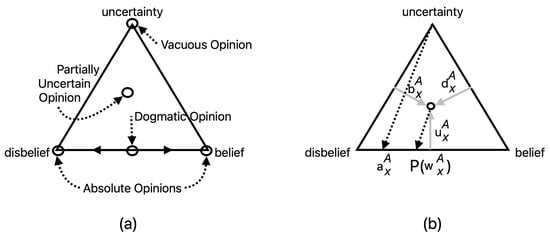
Figure 1.
(a) Subjective opinion triangle with the three vertices labeled corresponding to the belief, disbelief and uncertainty components of an opinion. The types of opinions are shown as open symbols with an associated name and connecting line. (b) The subjective triangle showing a single, partially uncertain opinion of source A regarding the classification of a sample as belonging to state x. The belief, disbelief and uncertainty values of source A regarding membership in class x (, , ) are shown in gray arrows. The dashed arrow going from the u-vertex to the value of the base rate () is the director line. The partially uncertain opinion is projected along a projector line parallel to the director line to a point on the base of the triangle corresponding to the expectation value of the opinion ), see text.
Formulating an ML subjective opinion can be accomplished by fitting predicted posterior probabilities from an ensemble of ML models to an appropriate probability distribution function. In the case of a binary opinion between two mutually exclusive states, the appropriate probability distribution is a beta distribution [5]. If the distribution of posterior probabilities for a sample is narrow the uncertainty is low, and as the width of the distribution increases, so does the uncertainty. This basic construct extends Dempster–Shaffer Evidence Theory [6]. The basis for the ensemble approach used here is briefly discussed in Section 2.5.
There is an important distinction between an “opinion” and a “decision” in classification problems, as discussed in Section 2.5. When the uncertainty mass goes to zero in a subjective opinion, the opinion becomes either an “absolute opinion” or a “dogmatic opinion”, see Figure 1. Nonetheless, the absolute or dogmatic opinion remains designated as a “subjective opinion”. Metrics such as true positive and false positive rates, accuracy, etc., are not defined for opinions. Determining the performance metrics for a classification method, ML or otherwise, requires a ground truth validation data set and a process of making a “decision” regarding the assignment of each validation sample to a class. Decisions are based on opinions. The process utilized in this work proceeds from an opinion to a decision is discussed in Section 2.6.
Access to large ground truth training data remains a challenge in some forensic science disciplines, as well as in some other areas where ML may be helpful. Training ML methods on in silico fire debris data with subsequent prediction of experimental validation data has previously been published [7,8]. As described in previous work, each single fire debris data record is generated from a linear combination of gas chromatography–mass spectrometry (GC-MS) data from a single ignitable liquid (IL) with the pyrolysis GC-MS data from one or more common building materials and/or household furnishings. Results from co-pyrolysis of polymers, biomaterials and mixtures provide fundamental data that reinforces the choice of a linear combination model, as does recent success using these in silico data for training multiple ML methods [8,9,10,11]. The in silico data from the previous work are freely available online, accessed 1 April 2025 (https://ilrc.ucf.edu) and will be utilized here in the context of this publication.
2. Background
2.1. Fire Debris Analysis
Fire debris analysis is an important and challenging area in forensic science. The main goal of fire debris analysis is to identify the presence or absence of an ignitable liquid residue (ILR) in samples collected from a fire scene. The analysis is typically carried out following the current ASTM E1618-19 protocol [12]. The analyst uses target compounds identified by GC-MS, extracted ion profiles (EIP), and chromatographic patterns to identify the presence of ILR in a sample. Some classes of ignitable liquid, as defined in the ASTM E1618-19 standard, have a characteristic chromatographic pattern, which can move throughout the chromatogram depending on the range of molecular weights (i.e., heavy, medium or light). Some classes are defined by components (i.e., those containing a significant oxygenated component, normal alkanes, aromatics, naphthenic-paraffinic and isoparaffinics), some are product specific (i.e., gasoline), while processing defines the petroleum distillate class, and the miscellaneous class corresponds to mixtures of liquids from several classes, single components, and any ignitable liquid (IL) not belonging to another defined class.
The ASTM E1618-19 reporting protocol requires an opinion expressed as a categorical statement regarding whether the sample contains ILR or not. Reporting in categorical statements corresponds to the analyst either reporting a “decision” or expressing an “absolute opinion”, see Figure 1 and Section 2.5. In the terminology of subjective opinions, an “absolute opinion” implies total belief or disbelief and no accompanying uncertainty. The absence of uncertainty does not reflect the reality of the analysis of complex fire debris samples. A positive determination is based on the identification of ILR belonging to a defined class [12]. Partial evaporation (i.e., weathering) of the IL during the fire and possible biological degradation after the fire can complicate the identification of ILR patterns. In addition, pyrolysis of building materials and furnishings under the high temperatures of the fire produces interfering background chemical components that can mask the presence of ILR. In summary, fire debris analysis is a complicated pattern recognition process that under current practice is entirely based on the interpretation of the analyst, is subjective, and prone to bias. Fire debris analysis is a task that could potentially benefit from ML classification. The reporting protocol given in the ASTM E1618-19 standard does not use a statistical metric to describe the strength of the evidence and does not promote the use of ML methods to assist the analyst [12]. In a 2009 report, the National Academy of Sciences (NAS) recommended using language in reports and testimony that conveys proper confidence or significance [13]. The European Network of Forensic Science Institutes (ENFSI) embraces evaluative reporting, which emphasizes the likelihood ratio as a measure of the strength of evidence [14,15]. The application of likelihood ratios in glass evidence [16] and fire debris analysis [7,8] is increasingly used in academic research.
2.2. Expert Opinions
In the United States, the Federal Rules of Evidence allow individuals qualified by specialized skill or knowledge to assist the courts as expert witnesses [17,18]. Fire debris analysts meet the requirements of expert witnesses. The expert witness is allowed to testify in the form of an opinion, as long as the testimony is helpful to the court and meets other requirements outlined primarily in Article VII of the Federal Rules of Evidence [18]. The focus of the work reported here, as it relates to forensic science, is on the analyst’s formulation of an opinion with the assistance of ML methods also designed to provide an opinion. Machine learning is presented with the intent of assisting the forensic scientist, not replacing them. Research on applications of ML in forensic science are finding their way into peer-reviewed publications [19,20,21].
Classification based on pattern data, including those created in silico by data imputation methods [7], can facilitate the use of ML in the forensic analysis of fire debris data [8]. Binary classification of fire debris samples as containing or not containing ILR has been demonstrated using decision theory and receiver operating characteristic (ROC) analysis to determine the evidential strength of a fire debris sample as a likelihood ratio and establish a classification/decision threshold for determining that a sample is positive for ILR. Machine learning methods have been used to calculate the posterior probability of ILR in a sample, from which the likelihood ratio can be obtained using the odds-form of Bayes’ equation and the prior odds of the two classes reflected in the training data. The ML methods that have been applied to this problem include support vector machines, partial least squares discriminant analysis, convolutional neural networks, k-nearest neighbors, logistic regression, XGBoost, and backpropagation neural networks [7,8,22].
2.3. Limitations to Machine Learning Predictions
The ML methods referred to in Section 2.2 can assist the analyst in assigning evidential strength in the form of a likelihood ratio. Decision theory, ROC analysis and ML can assist the analyst in making a decision; however, as discussed above, the analyst should be reporting an opinion [23], not a “forensic decision”. Complex ML methods, when presented with previously unseen data for the purpose of prediction, typically give a single answer (e.g., the posterior probability that a sample contains ILR). If the new data lies outside the distribution of the training data, or if the training set was too small to accurately represent the state space, the predicted probability may lead to an erroneous categorical classification due to uncertainty in the prediction. Uncertainty falls into three categories, aleatoric, epistemic and distributional [2]. Aleatoric uncertainty is comprised of data uncertainty, such as label noise and class overlap. Epistemic uncertainty arises from model complexity, and distributional uncertainty is due to training-testing set distribution mismatch. The epistemic uncertainty can be reduced by increasing the size of the training data set; however, the aleatoric uncertainty is not reduced by increasing the size of the training data set. If the model’s probabilistic output is converted to a categorical value for forensic reporting (e.g., reporting an absolute opinion as ILR present or not), the effects of uncertainty are more significant. Opinions reflecting unacceptable levels of uncertainty should not be used for making decisions, and therefore a knowledge of the uncertainty associated with each opinion is required.
The use of databases containing records of IL and substrate pyrolysis data is supported under the current ASTM standard [12]. Databases are retained by most fire debris analysis laboratories. A set of data is also freely available online from the National Center for Forensic Science (NCFS) at the University of Central Florida (UCF) [24]. The NCFS site also contains fire debris data sets generated in-silico, 240,000 samples in total, for use in ML applications. Experimental ground truth fire debris data set for ML validation is also available on the NCFS site. The work reported here uses 60,000 in-silico training samples and 1117 ground-truth validation samples from the NCFS site. The ML method predictions from an ensemble of models are fused using the principles of subjective logic to provide the analyst with an “opinion”, not a single answer [1,5,25,26,27]. In this approach, the formalism of subjective binary opinions is used as a fusion method for the ML outputs in a way that is similar to the fusion step in ensemble methods.
2.4. Ensemble Methods
While single ML models give a single output, multiple models may be combined into an ensemble learner [28,29].
“The main premise of ensemble learning is that by combining multiple models, the errors of a single inducer will likely be compensated by other inducers, and as a result, the overall prediction performance of the ensemble would be better than that of a single inducer.” [28]
Ensemble learning models fuse the output from a series of base models (i.e., ML models, also called “inducers”) to produce a single output. Weighting methods, such as majority voting, are commonly applied in classification problems by assigning the final classification to the class receiving the most votes from the evenly weighted ensemble base models [28]. Another weighting approach is to assign weights to the base models in proportion to their performance on a validation data set. Other weighting methods have been reviewed by Sagi et al. [28]. Construction of the ensemble can be done in such a way as to make each successive base model dependent on the previously created base models (i.e., the dependent framework) or by creating each base model so that it is independent of the other base models (i.e., the independent framework) [28]. Common dependent frameworks include AdaBoost and gradient boosting, while popular independent frameworks include bagging and random forest methods. In the work reported here, ensembles of three ML base models are examined: (1) linear discriminant analysis (LDA), (2) random forest (RF) and (3) support vector machines (SVM). In each case, the base model output is fused to provide a distribution of class membership probabilities. The probabilities from each approach are fitted to a beta distribution. From the beta distribution fitting parameters ( and ), a subjective opinion is created. The motivation for this approach is the need for the ML method to provide an opinion with the associated belief, disbelief and uncertainty masses for each sample. The ML opinion is consistent with the need of the analyst and courts, and therefore is more useful to the analyst than a single answer and a confidence interval.
2.5. Subjective Opinions from Machine Learning
The research presented here is based on previous work by Sensoy [30], Ghesu [2], Tong [31], Jøsang [5] and Whitehead [1]. It is useful in forensic science and legal questions to consider two mutually exclusive competing propositions. This approach facilitates taking a probabilistic likelihood ratio approach which is popular in evaluative reporting [15]. The likelihood ratio is equivalent to the slope of the tangent to an ROC curve at any point on the curve. Setting a threshold on the ROC curve is required for making decisions, but not for formulating a subjective opinion or approximating a likelihood ratio. In this work, fire debris samples are classified into two mutually exclusive competing states of containing ILR, denoted state x, or not containing ILR, denoted state , which allows the fusion of the output from multiple ML methods to form a frame of discernment. The binomial subjective opinion that a sample belongs to state x based on the ML results is denoted as, . The opinion is written as an ordered tuple
In Equation (1), expresses to the belief that a sample belongs to state x, expresses the disbelief in the proposition, expresses the uncertainty, and represents the base rate for x in the population. For a binary frame of discernment, is typically assumed to have a value of 0.5 (i.e., the uninformative prior) in the absence of other specific information. The belief, disbelief and uncertainty must sum to one, as shown in Equation (2).
The values of the belief and disbelief are calculated from the shape parameters derived from fitting the set of ML posterior probabilities that a sample belongs to class x to a beta distribution. The fitting parameters are and , and the equations for calculating the belief and disbelief are given in Equations (3) and (4). (NOTE: Ghesu states and > 1. This is not a requirement for a beta distribution, only that the values are positive real numbers.)
The uncertainty can be calculated from Equation (2), after calculating the belief and disbelief from Equations (3) and (4). The projected probability function for the opinion is given in Equation (5).
The projected probability corresponds to adjusted by a portion of the base rate, as determined by [5]. The value provides an estimate of how the probability of x varies from the base rate. The projected probability “unifies all of the opinion parameters in a single probability distribution and thus enables reasoning about subjective opinions in the classical probability theory” [5]. It is possible to recover the fitted beta distribution from using Equation (6). See [1] for examples of how probability distributions correspond to subjective opinions.
2.6. Decisions and Strength of Evidence from Opinions
The ML opinion ensemble method outlined in Section 2.5 can be extended if the application requires a decision, or if the analyst would like to express the strength of the evidence as a likelihood ratio. The process of proceeding from a set of ML subjective opinions to an ROC curve is described in this section. The basic approach is to obtain the values from a set of validation data with known ground truth. The uncertainty lies in the opinion, whereas the values are probabilities and follow the rules of probability calculus. The values can be used to calculate likelihood ratios which serve as scores for generating an ROC curve. Uncertainty in the opinion does not imply uncertainty in the likelihood ratio which is consistent with Taroni et al. [32].
A first step, though not required, is to decide on a maximum allowed opinion uncertainty for samples that require a decision. All samples having greater than the cutoff would be considered too uncertain based on the ML to proceed with a decision, where to set the limit would depend on the application and organizational standards and protocols.
Decisions in binary cases can be made based on a decision threshold which can be plotted on the ROC curve. An optimal decision threshold score allows control over the false positive rate while simultaneously setting a true positive rate [31]. Creating an ROC curve requires the analysis of known ground truth validation samples and the creation of a “score” which is proportional to the probability that the sample belongs to the positive class [33,34]. In this work, the log-likelihood ratio (LLR), Equation (9), based on the projected opinion has been used as a score for creating an ROC curve. The higher the score, the more likely it is that the sample belongs to class x.
The likelihood ratio can also be determined from the slope of a tangent to the ROC curve [35] at any point on the curve, irrespective of the score definition. However, it is important that classifications and the probabilities they are based on are calibrated. One popular method of calibrating probabilities, based on isotonic regression, is the pooled adjacent violator (PAV) algorithm. The PAV-calibrated probabilities can be obtained directly from the slopes of covering segments of the ROC convex hull (CH) [36]. Once the ROC curve is created and the convex hull is calculated, the for any previously unseen sample (e.g., a casework sample) can be used to calculate the likelihood ratio and the slope of the covering segment of the ROC CH gives the calibrated strength of the evidence.
The equation for the likelihood ratio is obtained by rearranging the odds form of the Bayes equation, Equation (7), and making the appropriate substitutions. In Equation (7), is the proposition that ILR is present, is the proposition that ILR is not present and E is the evidence, which in the current context is the set of normalized relative intensities of the ions from feature selection, see Table 1. The term is the posterior odds, is the likelihood ratio and is the prior odds.

Table 1.
Relevant mass-to-charge (m/z) ratios retained and removed during feature selection.
The projected probability of the opinion, , is calculated by Equation (5), see Section 2.5. Rearranging Equation (7) to isolate the likelihood ratio and substituting for , for , for and for , the expression for the likelihood ratio, Equation (8), is obtained. Taking the base-10 logarithm of Equation (8) gives the log-likelihood ratio (LLR), Equation (9). The calculated LLR values, combined with the known ground-truth class membership of the validation samples, were used to generate ROC curves.
3. Materials and Methods
3.1. Data Pre-Treatment
A data set of 60,000 in silico total ion spectra (TIS) [37] of fire debris samples was used to train each ensemble of LDA, random forest (RF) and support vector machine (SVM) models [7]. The total ion spectrum is analogous to the total ion chromatogram; however, the mass spectral data is averaged across the entire chromatographic profile and normalized to the most intense peak. The TIS allows comparison of 70 eV electron ionization mass spectral data collected on a low-resolution instrument with linear quadrupole mass analyzers across different laboratories without accounting for chromatographic peak shifts. The in silico data set contains 30,000 samples with ILR (class x) and 30,000 without ILR (class ). The LDA, RF, and SVM methodologies are supervised ML techniques that can be used for classification [8]. The validation/test data set contains 1117 laboratory-generated known ground truth fire debris samples. Testing on casework or “real” fire debris is not included because the ground truth for these samples is not known. The TIS contain the mass to charge ratios (m/z) from 30 to 160. The baseline m/z 32 and 76 ions were removed from the training and test data before initiating the calculations. The m/z ratios provided in Table 2 in ASTM E1618-19 [12] were selected as initial features based on their chemical importance to ILR identification in fire debris [12]. Further feature selection was conducted by removing ions with zero variance and those with correlations greater than 0.9 from the in silico data set. The data sets were normalized to the most abundant (i.e., most intense) m/z value remaining after feature selection. Pretreatment and feature selection left 26 ions, see Table 1 for training and validation of each ML method. An ensemble of models () for each machine learning technique (LDA, RF and SVM) was trained independently using randomly selected samples of sizes (n = 100, 200, 1000, 2000, 20,000, and 60,000) of in silico data. The n samples for each of the m ensembles were selected randomly with replacement (i.e., bootstrapped) from the data set of 60,000 in silico samples. The n samples for each training set were selected to retain a class balance, and . All calculations were performed using R, version 4.5.0 [38].
3.2. LDA, RF and SVM Models
The random forest training was performed using the package “randomForest” in R [39]. The number of random regression trees selected for this calculation was set to 500. The number of regression trees was based on the best performance of random forest models containing 500, 1000, 1500 and 2000 regression trees trained on the 60,000 in silico data set and tested on the 1117 validation samples. Subsequent training of each of the 100 models comprising the ensemble was done holding the number of regression trees at 500 and optimizing the “mtry” parameter (i.e., the number of features randomly sampled as candidates at each split in a tree), using the “tuneRF” function [39]. The initial mtry value was set at 5 with increments of 2 for mtry. For each ensemble, 100 random forest models were trained on in silico training sets that were constructed by bootstrapping 100 training data sets. The number of in silico samples in the ensembles was varied to 100, 1000, 2000, 20,000 and 60,000. The size of the training data sets was changed to test for the effects of training sample size on model uncertainty. The posterior probability of the presence of IL in each fire debris sample was calculated using each of the ensemble members. The calculated probabilities were fitted to a beta distribution. The fitting was performed using the “fitdistrplus” package in R [40]. The fitting parameters ( and ) from the beta distribution were then used to calculate , , and for each fire debris validation sample using Equations (2)–(4), and was calculated by Equation (5) with ; see Section 2.5.
LDA was executed using the “MASS” package in R using the “lda” function [41], and the priors were set to 0.5 for each class x and . The LDA method does not have adjustable parameters for optimization. The probability of the presence of IL in each fire debris sample of the validation data set was predicted by applying the LDA ensemble models. These probabilities were then used to fit the beta distribution ( probabilities for each fire debris validation sample). The beta distribution fitting was implemented using the “fitdistrplus” package in R [40]. The fitting parameters ( and ) from the beta distribution were then used to calculate , , and for each fire debris validation sample using Equations (2)–(4), and was calculated by Equation (5) with ; see Section 2.5.
The SVM calculations were executed using the “caret” package in R [42]. The values of the fitting parameters C and were optimized by a grid search varying C from 0.1 to 2 in 5 steps and varying from 0.01 to 0.5 in 5 steps. Parameter optimization was performed on a randomly selected subset of 3000 class x and 3000 class samples. The fitting parameters and were held constant for subsequent training of each of the 100 SVM base models on in silico training sets of 100, 1000, 2000 and 20,000 samples. The probability of the presence of IL in each fire debris sample of the validation data set was predicted by applying the SVM ensemble models and fitting the set of posterior probabilities to a beta distribution as described for the RF and LDA methods.
4. Results
4.1. Beta Distribution Assumptions
The theory of binary subjective logic is well established [5]. The two mutually exclusive and comprehensive states represent a Bernoulli distribution and the conjugate prior is a beta distribution. However, the ML methods applied as ensembles are not guaranteed to produce a set of predicted probabilities of class membership that fit a beta distribution. Tests of the beta distribution were made by the Kolmogorov–Smirnov distance (D) statistical test (i.e., the K-S test) [43]. The test statistic compares the empirical cumulative probability distribution to the cumulative probabilities for the reference beta distribution. The reference beta distribution is based on the fitted and shape parameters for each validation sample. The Null hypothesis is that the empirical distribution was drawn from the reference distribution. If the measured statistic is greater than the critical value, , the Null hypothesis is rejected. The critical value is [43].
Table 2 gives the results for the K-S test on the beta distribution fitting data for LDA, RF and SVM base models. The “Samples” column gives the number of in silico samples used to train each of the 100 ensembles. The “Mean D” column gives the average value of D calculated for the 1117 validation samples. The “Non-Beta Fits” and “% Non-Beta Fits” columns give the number and percentage, respectively, of the 1117 samples where the predicted probabilities of class x membership were statistically different from a beta distribution at the significance level. Increasing the training set size for the LDA models improved the fraction of validation samples that fit a beta distribution. The RF ML models showed the opposite trend, with an increasing number of validation samples’ predicted class membership probabilities not conforming to a beta distribution. This trend is not understood, nonetheless, the percentage of non-beta distributions remained below up to a training set size of 2000. However, as the size of the RF training set increased, the median uncertainty showed statistically significant improvement and the ROC AUC also exhibited statistically significant improvement up to a training set size of 60,000. These trends are discussed further in Section 4.2, Table 3 and Table 4. The decreasing median uncertainty for indicates a narrowing of the fitted beta distribution which results from increased similarity among the predicted probabilities from all members of the ensemble. The SVM ML models gave the poorest performance regarding the beta distribution fit. The further analysis of the observed trend for the RF base models will be studied in the future as it is beyond the scope of this work.
Table 2.
Beta distribution fitting data for LDA, RF and SVM base models. The “Samples” column contains the number of in silico samples in a training data set. The “Mean D” column contains the mean Kolmogorov–Smirnov distance statistic for the beta distribution fit of probabilities of class x membership for each of the 1117 validation samples fitted. The “Non-Beta” and “% Non-Beta” columns contain the number of validation samples and the percent of validation samples respectively that failed the two-sided hypothesis test (, ). The Null hypothesis for the test was that the experimental data was drawn from a beta distribution defined by the best fitted and shape parameters.
Table 3.
Uncertainty results for validation of LDA, RF and SVM base models, The “Samples” column contains the number of in silico samples in a training data set. The “Bimodal” column contains the number of bimodal beta distributions that resulted from fitting the ML-predicted probabililty of membership in class x. The “Median ” and “Max. ” columns contain the median and maximum uncertainty, respectively, for the validation opinions. The “Wilcoxon p” column contains the p-values for Wilcoxon rank sum test comparison of the median uncertainty for a ML method and training sample size with the median uncertainty from the sample-size row above.
Table 4.
The ROC AUC results for LDA, RF and SVM base models. The “Samples” column contains the number of in-silico samples in a training data set. The “AUCs,m,w” contains the ROC AUC for all of the validation samples (i.e., those with strong, moderate and weak IL/SUB ratios). The “95% CI” column contains the confidence interval for the ROC AUCs,m,w of validation samples. The “p-Value” column contains the p-values for Delong test comparing the ROC curves for a ML method and training sample size with the ROC curve from the sample-size row above.
4.2. Training Data Set Size Effects
The results from varying the total number of samples in the training data set are shown in Table 3 and Table 4. The total number of samples (first column) in each case consists of an equal number of samples containing ILR (class x), and samples containing no ILR (class ). Data sets with equal representation from classes x and are balanced. The number of base models in each ensemble was 100. The results shown in the “Bimodal” column in Table 3 reflect the number of the 1117 validation samples that produced a set of posterior probabilities that were best fitted by a beta distribution with both and less than 1, which corresponds to a bimodal distribution. In the LDA model, training data sets composed of 2000 randomly chosen samples were required to eliminate the bimodal fits. When the beta distribution fit parameters for a single validation sample both fell below a value of 1, the model was considered as showing significant uncertainty. In those cases, the values each fitting parameter were assigned a value of 1, which results in of 1 and each of and equal to 0. In contrast, even the minimum training data set sample size (50 x and 50 ) did not produce bimodal posterior probability distributions from the ensemble of RF and SVM models. This is attributed to the greater complexity of these models. The RF models each contained 500 trees and optimized the mtry parameter. The SVM models produce a complex support vector with tuning parameter `sigma’ held constant at a value of 0.1325 and tuning parameter `C’ was held constant at a value of 2.
The “Median ” column in Table 3 provides the median value obtained for the 1117 validation samples. The “Max. ” column gives the maximum uncertainty from the validation opinions. The Wilcoxon rank sum test was applied to each successive sample size to determine if the median was statistically decreasing as the number of training samples increased. The Wilcoxon p-value is given in the last column of Table 3. The p-values were very small and indicate that the decreases in median were statistically significant. Shapiro–Wilk normality tests showed the values were not normally distributed in each case. The Wilcoxon rank sum test is non-parametric and does not rely on an assumption of normality.
The LDA results show a maximum of total uncertainty, , for some validation samples predicted with models developed with training data sets of 1000 or less samples. The maximum uncertainty of the LDA model ensemble falls to a very low value of 5.60 at a training data set size of 60,000 samples. The training samples were bootstrapped to ensure that all 100 training sets were not equivalent. The very low uncertainty for the LDA base model is attributed to the in silico data creation method [7] which mixes IL into SUB at varying contributions. The covariances for x and are nearly identical, which is a requirement for the LDA model; however, the training data set size must be large enough to sufficiently represent the validation data. The low uncertainty of the LDA base model does not necessarily mean that the model discriminates well between x and classes.
By comparison, maximum uncertainty for the RF model, , starts at 3.52 for the smallest training data sets and decreases to 1.20 for the largest training size. The RF is a much more sophisticated ML model than LDA; however, the slightly larger value, in comparison to , indicates that the RF ML models are giving slightly broader distribution of the posterior probabilities of class x membership. The same trend can be seen in the median values for and .
The SVM models gave larger median and maximum values than either the LDA or RF methods. This is attributed to the complexity of the support vectors for each ensemble member, which results in a larger range of posterior probabilities of class x membership for each validation sample predicted by each of the 100 ensemble members.
The last three columns of Table 4 directly address the class separation performance on the fire debris validation data by the three ML models as a function of training data set size. The is the area under the ROC curve generated from all validation samples. The subscripts on indicate the relative contribution (strong, moderate and weak) of the ILR in the fire debris validation samples. The ratio was calculated from the most intense chromatographic peaks corresponding to IL and SUB contributions. Ratios of IL/SUB correspond to , and . The AUC is equivalent to the probability that a randomly selected x sample will have a greater score than a randomly selected sample. A higher AUC corresponds to better class separation.
In Table 4, the “95% CI” column gives the confidence interval for the AUC and the “p-value” column gives the statistic for the two-sided Delong test. The LDA ROC curves are not statistically improving for models exceeding 200 training samples. The RF ROC curves did not statistically improve for models exceeding 20,000 training samples. The SVM ROC curves continued to get statistically better for models up to 20,000 training samples. The SVM ML was not applied to models exceeding 20,000 training samples due to limited computational facilities.
Table 5 shows the change in ROC AUC as the size of the training set increased and the ratio of IL/SUB was changed. For all three ML models, at all training data set sizes, the AUC is seen to increase as the IL/SUB ratio incorporated into the model goes from all samples in the second column from the left (i.e., ) to only the high IL/SUB ratio (i.e., ) in the rightmost column. The standard error for each AUC is given in parentheses. The increase in AUC at each training sample size, proceeding from to , and from to is statistically significant based on a Delong test, with each p < 2.2 . This result demonstrates that both ML methods are producing better class separation at strong ILR contribution. Notably, at even the smallest training size, the RF model produces better class separation than the LDA model at the largest training size. At the largest training size, the RF model produces an AUCs,m,w of 0.849, and the AUCs of 0.962 indicates very good class separation. The SVM ML model is producing a similar AUC to the RF ML model at a training size of 20,000.
Table 5.
Comparison of the ROC curves as the IL relative contribution is increased. The “Samples” column contains the number of in-silico samples in a training data set. The “AUCs,m,w” column contains the ROC AUC for all validation samples. The “AUCs,m” column contains the ROC AUC for validation samples having strong and moderate IL contributions. The “AUCs” column contains the ROC AUC for validation samples having strong IL contributions. The standard error for each AUC is given in parentheses. Strong, moderate and weak IL contributions are defined in the text.
All models are performing similarly to what would be expected from a human analyst (i.e., better ILR detection as the ILR relative contribution increases). The most significant differences in the models are the excessive uncertainty produced by LDA at very small training sizes, the higher overall uncertainty by SVM, and the long training times required by SVM. The optimal model studied in this research is the RF ensemble trained on 60,000 training samples.
4.3. Visualizing Opinions and Performance
As shown in Figure 1, the visualization of binary subjective opinions is possible in a ternary plot. The calculated values for the validation samples trained on 1000 x and 1000 samples are shown in Figure 2. Figure 2a shows the values for validation samples belonging to class , and the plot Figure 2b shows the values for validation samples belonging to class x. The plots allow an immediate visual assessment of for any sample. Other general trends are observed from the ternary plots in Figure 2. The value for some of the validation samples belonging to class x are larger than some of the class . The three class x samples with the highest values all contained moderate or strong levels of the same aromatic solvent that had been weathered to 75% loss of volume, and they all contained “glue stick” as one of the substrate components. The samples correspond to reference numbers 694, 695 and 696 in the Fire Debris Database [24]. In this case, the identity and composition of the samples with the highest predicted uncertainty do not assist in understanding shortcomings in the LDA ML model, but the information could be helpful to the forensic science interpretation of model performance.
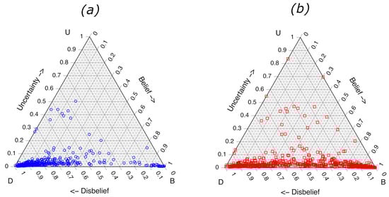
Figure 2.
Ternary diagrams showing LDA subjective opinions for 1117 experimental validation fire debris samples. (a) Samples containing no ILR and (b) samples containing ILR. Opinions based on 100 LDA models, each comprised of 2000 training samples (1000 containing ILR and 1000 containing only substrate pyrolysis components).
It is also evident from the plots that the , generated from the projection of each point straight down onto the bottom axis (due to ) results in substantial overlap of the two classes. A quantitative analysis of the extent of class separation requires visualizing the values on an ROC graph.
The values for the binary opinions were used to calculate scores to generate an ROC curve. The ROC curve resulting from the LDA ensemble trained on 2000 samples, including strong, moderate and weak IL contributions, is shown in Figure 3. The corresponding is 0.789, see Table 4.
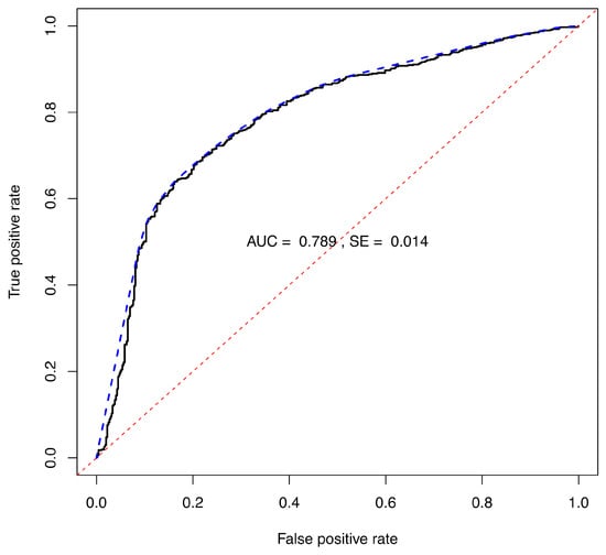
Figure 3.
ROC diagram based on the LLR for the projected opinions for each of the 1117 experimental validation fire debris samples from Figure 2. The ROC curve is shown as a solid line. The ROC CH is shown as a blue dashed line, and the random guess curve is shown as the red dashed line. The ROC is 0.789.
The ternary plots and ROC curve for the RF model trained with 2000 samples in each of the 100 base-models of the ensemble are shown in Figure 4 and Figure 5, respectively. The ternary plots demonstrate the lower uncertainties arising from the RF model, with the highest value of approximately 0.20–0.30 calculated for several of the class samples. The largest uncertainties for the x samples were approximately 0.20. Again, the values are obtained by projecting each point straight down to the base of the ternary plot (). The class separation of the LLR scores calculated from the values, Equation (9) produces an ROC plot, as shown in Figure 5, with an of 0.837, as well as Table 4.
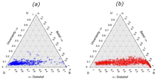
Figure 4.
Ternary diagrams showing RF subjective opinions for 1117 experimental validation fire debris samples. (a) Samples containing no ILR and (b) samples containing ILR. Opinions based on 100 RF models, each comprised of 2000 training samples (1000 containing ILR and 1000 containing only substrate pyrolysis components).
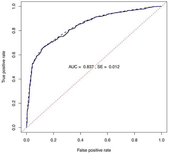
Figure 5.
ROC diagram based on the LLR for the projected opinions for each of the 1117 experimental validation fire debris samples from Figure 4. The ROC curve is shown as a solid line. The ROC CH is shown as a blue dashed line, and the random guess curve is shown as the red dashed line. The ROC of 0.837.
Increasing the number of samples in each training set leads to a further decrease in the median and maximum observed , as shown in Table 3. The maximum observed plateaus around a value of 0.1, as shown in Table 3. The ternary plots for the models trained on 20,000 in silico samples for each member of the ensemble are shown in Figure 6. Although increasing the training sample size decreases the maximum observed , the ROC only increases to 0.846, as shown in Table 3. Similar results are observed for the LDA method.
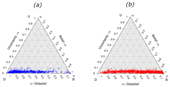
Figure 6.
Ternary diagrams showing RF subjective opinions for 1117 experimental validation fire debris samples. (a) Samples containing no ILR and (b) samples containing ILR. Opinions based on 100 RF models, each comprised of 20,000 training samples (10,000 containing ILR and 10,000 containing only substrate pyrolysis components).
4.4. Extending the Opinions to Classification Decisions and Evidentiary Value
This approach is demonstrated for the RF base-method where each ensemble member is trained on 2000 in silico samples. An uncertainty opinion threshold was set at 0.10 for this example. The threshold is subjective and should be adjusted based on the amount of uncertainty the application can tolerate. By setting a threshold of 0.10, many of the 1117 validation samples are determined to be ineligible for a decision. The opinions of the 795 validation samples that are decision eligible are shown in Figure 7. The ROC curve that was generated from the decision eligible validation samples is shown in Figure 8. The ROC AUC for the curve in Figure 8 has decreased slightly from 0.837, see Table 3, to 0.832. The LLR decision threshold of 0.07 was obtained by setting the maximum false positive rate at 0.05, which corresponds to the Neyman–Pearson value. Projecting vertically from a false positive rate of 0.05, the score at the point of intersection with the ROC curve is the decision threshold LLR of 0.07. The decision LLR corresponds to a of 0.54 in the ternary plots. Projecting from the decision threshold horizontally to the true positive rate axis gives an intersection of 0.55, which is equal to the quantity , where is the Neyman–Pearson value of 0.45.
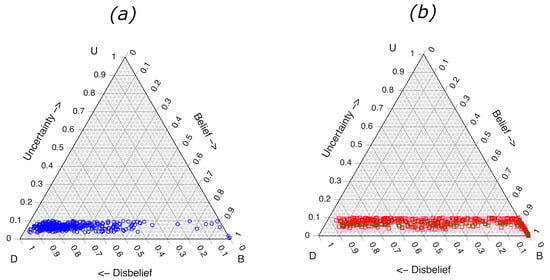
Figure 7.
Ternary diagrams showing RF subjective opinions for 795 validation fire debris samples with calculated . These low uncertainty opinions were selected from RF calculations comprised of 2000 training samples for each of 100 RF base models. (a) Samples containing no ILR and (b) samples containing ILR.
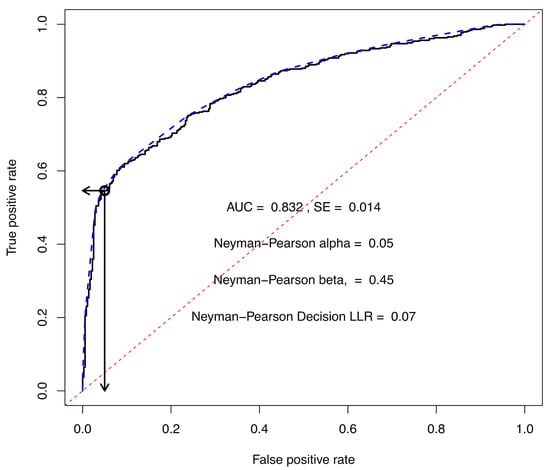
Figure 8.
ROC diagram based on the LLR for the projected opinions for each of the 795 validation fire debris samples having an from Figure 7. The ROC curve is shown as a solid line and the ROC convex hull (CH) is shown as a blue dashed line on the upper and left edge of the ROC curve, and the random guess curve is shown as the red dashed line. The ROC of 0.832, with a standard error of 0.014, is labeled on the graph, along with the decision threshold based on a Neyman–Pearson (solid black arrow pointing down), and corresponding . The left-pointing solid black arrow points to . The decision threshold, shown as an open circle on the ROC curve corresponds to an . The is the corresponding decision threshold on the ternary diagrams, see Equation (9).
The significance of Figure 7 and Figure 8 is that a previously unseen sample with a calculated from the same model may be classified as belonging to class x or class with known true and false positive rates. Samples with should be classified into class x, only if a decision is required. Otherwise the analyst should be reporting an opinion, which may include the strength of the evidence expressed as a likelihood ratio.
Although a 5% false positive rate is often employed in hypothesis testing, it can be argued that a 5% false positive rate in forensic science could call into question the admissibility of the evidence. Obtaining a validated false positive rate in fire debris analysis is difficult due in part to the challenge of obtaining casework-realistic ground truth samples. Sampat at al. reported an 89% true positive rate for IL detection and a 7% false positive rate for tests limited to three classes of IL while using two-dimensional gas chromatography with time-of-flight mass spectrometry [44]. When setting a decision threshold on an ROC curve, a lower false positive rate will correspond to a lower true positive rate. This trade-off becomes less problematic as the ROC AUC increases.
The calibrated likelihood ratio for any point can be determined from the slopes of the covering segment of the ROC CH. The ROC CH in Figure 8 comprises 20 segments, as shown in Table 6. For example, if a sample is calculated to have a , it would meet the eligibility requirement for proceeding to a decision if a decision were required. Further, if the sample had a , the score calculated from Equation (9) would be 0.421. The calculated score is greater than the Neyman–Pearson decision score of 0.07, as shown in Figure 8, and would be classified as belonging to class x. The calculated score would fall between points 3 and 4 in Table 6 and would be covered by segment 3. The calibrated LR for the sample would be 12.715 (). This procedure can be followed for any sample in this work that was calculated by the RF model trained on 2000 balanced in silico samples for each of the 100 ensemble RF base-functions.
Table 6.
Convex hull segments corresponding to the ROC curve CH shown in Figure 8. The left-most column assigns a number to the points on the CH, starting at the bottom of the plot, coordinate (0,0) and moving up. The second column from the left assigns a number to each covering segment of the CH, i.e., the segment between points 1 and 2 is labeled as segment 1. All scores greater than or equal to a value of 2.489 (see column 5) are “covered by” covering segment 1. The next two columns give the false positive rate (FPR) and true positive rate (TPR) coordinates for each point on the ROC CH. The third column gives the score corresponding to each ROC CH point. The rightmost column corresponds to the LR (i.e., the slope) of the associated covering segment. The slope of each segment corresponds to the PAV calibrated likelihood ratio of all points on the ROC curve which are covered by the CH segment.
5. Discussion
5.1. Advantages of the ML Opinion Method
The method of interpreting an ensemble of ML methods discussed in this paper provides an opinion, as opposed to a single numerical value. The method provides important insight into the level of opinion uncertainty for individual samples as determined from the ensemble of base-models. Uncertainty is associated with each sample’s opinion, which stands in contrast to a confidence based on the average cumulative errors of all validation samples. The method is demonstrated here for a binary classification process; however, the subjective logic approach can be extended to a higher dimension through the use of the appropriate Dirichlet probability distribution function in place of the beta distribution. The reader is referred to [4,5].
The ML opinion can be taken into consideration by the expert when formulating their opinion. A knowledge of the uncertainty associated with ML opinions for each casework sample can allow the expert to give proper weight to ML calculations, thus limiting bias for or against the calculated result. Though not discussed here, it is possible to combine subjective opinions to obtain a consensus opinion, see [1]. These positive attributes apply to other applications areas where the results of a calculation could facilitate the formulation of an opinion. Areas such as self-driving vehicle control, medical image interpretation, military action/reaction considerations, etc., can benefit from additional advisement and opinion input into a decision process.
The methodology presented here focuses on binomial opinions regarding two comprehensive and mutually exclusive classes, which is frequently encountered in legal propositions, where an opinion is required. Even if a decision is required it should be based on an opinion. In binary cases, a decision can be generated from an ML opinion or a consensus opinion, based on an ROC curve and the associated CH as shown here. Similarly, the strength of evidence can be obtained from the ROC CH segments.
Visualization of a binary opinion in a ternary plot provides additional insight into model performance. Increasing the training sample size leads to some decrease in , as shown in Figure 4 and Figure 6. However, lower does not always correspond to a major increase in class separation (e.g., ROC increasing from 0.798 to 0.847 for the RF base model). Lowering reflects a narrowing distribution of the predicted posterior probabilities of class membership coming from all of the ensemble models (i.e., the opinions are becoming more dogmatic-like, see Figure 1). Limiting the IL contribution to increasingly larger values (i.e., less complicated samples) results in better class separation, as reflected in the increasing ROC AUC across a given training set size (e.g., , and for 20,000 training set size using the RF base model), see Table 3.
Increasing the size of the LDA and RF training sets is producing more dogmatic-like opinions for all samples, but not improving the model’s ability to distinguish between classes. A minimum size of the training data set of 2000 samples was required to avoid a binomial distribution of the ensemble of predicted probabilities that a single validation sample contained ILR. The potential use of in silico data to overcome a lack of experimental ground truth data in ML is demonstrated by this result. Binomial distributions were not observed for the other ML methods studied, even for training sets of 100 samples. Finding an ensemble base ML method that gives better class separation would increase the analyst’s confidence in the ML opinion.
5.2. Limitations of the ML Opinion Method
The computational resources required to implement this approach are not insignificant. The training time required for the ensemble of base models is large. In this work, the LDA and RF methods trained much faster than the SVM ML, as also previously reported [1]. The number of prediction calculations also exceeds the requirement for a single model (e.g., for a single RF model). Reducing the number of required prediction calculations has been addressed in the development of deep neural networks that are trained to output class or probability predictions as well as subjective logic parameters [4]; however, deep neural networks are computationally expensive to optimize and train. If the ensemble method is to be repeatedly applied to new samples over a period of time, the trained parameters of the ensemble base models must be stored, which also imposes a memory cost.
While the theory of subjective opinions for two comprehensive and exclusive classes is well established, the ML predicted probabilities of class membership do not fit a beta distribution for all validation samples. There is a need for understanding why some samples fail to fit a beta distribution for some ML models, yet the majority of samples examined in this work do fit the distribution. This is a topic for future work.
5.3. Future Work
While out-of-distribution detection has been demonstrated for single feature problems [2], the capability remains untested for this application. Research is needed to define and test for out-of-distribution samples (e.g., highly weathered debris, biologically degraded samples, unusual substrates, etc.). A study following the ML opinions for a series of in-silico samples starting with a strong unweathered IL and progressing to higher degrees of weathering and/or biological degradation would be informative. As the samples progress from in-distribution to outside the training distribution, the uncertainty would be expected to increase and the evidentiary value would be expected to decrease.
Additional research is needed to understand the influence of training set size and ML method on departures for some samples from a beta distribution for the predicted probabilities of class membership. Ideally, a sample can be found where the predicted probabilities of class membership fit a beta distribution for one training set size and fail to fit for a different training set size. Results of these tests will provide insight into how this violation of the theoretical basis alters the binomial subjective opinion.
The ternary diagrams of binary opinions are helpful in understanding the base model performance in this complicated fire debris analysis problem; however, more research is needed to determine the optimal interplay between , and to optimize interpretation of the ML opinion. What should the ternary opinion diagram look like for the validation data in a two state classification problem? How does the choice of base model and model overfitting affect the opinion distribution in the ternary diagram? A better understanding of the base model’s performance and influence on the opinion distribution will be more easily developed for the two state problem than the higher dimension problem. Expanding the approach to higher dimension problems will be met with new challenges of opinion visualization and interpretation; however, this is an essential direction of future research to make the approach applicable across a larger domain of problems.
6. Conclusions
A ML subjective opinion method has been demonstrated and applied to the problem of fire debris analysis. The effects of training data set size were shown for LDA, RF and SVM methods. The best ML method was found to be RF with an ensemble of 100 training sets, each composed of 20,000 in silico samples. All three ML methods studied were shown to give larger ROC AUC values as the validation data set was limited to larger IL contributions. In this sense, the method was exhibiting performance patterns that we would expect from a human analyst.
Author Contributions
Conceptualization, A.A. and M.E.S.; methodology, A.A. and M.E.S.; software, A.A. and M.E.S.; validation, A.A. and M.E.S.; formal analysis, A.A. and M.E.S.; investigation, A.A. and M.E.S.; resources, A.A. and M.E.S.; data curation, A.A.; writing—original draft preparation, A.A. and M.E.S.; writing—review and editing, A.A. and M.E.S.; visualization, M.E.S.; project administration, A.A. All authors have read and agreed to the published version of the manuscript.
Funding
This research received no external funding. Author M.E.S. is retired from the University of Central Florida (UCF), and received no compensation from UCF for this work.
Data Availability Statement
The data used in this study are freely available for download from the National Center for Forensic Science at: https://ilrc.ucf.edu/insilico-fire-debris-datasets/, accessed on 1 April 2025. The code is available from https://github.com/Rscriptsfiredebris/Uncertainty-calculations-Application-in-forensic-science.git (accessed on 28 July 2025).
Acknowledgments
During the preparation of this manuscript/study, the author(s) used Overleaf, accessed on 1 May 2025. https://www.overleaf.com for the purposes of collaborative authorship. The authors have reviewed and edited the output and take full responsibility for the content of this publication.
Conflicts of Interest
The authors declare no conflicts of interest.
Abbreviations
The following abbreviations are used in this manuscript:
| a | Base rate (general) |
| Base rate of class x by source A, | |
| ASTM | American Society of Testing Materials |
| AUC | Area Under the Curve |
| b | Belief mass |
| Belief mass for class x by source A, | |
| CH | Convex Hull |
| d | Disbelief mass |
| Disbelief mass for class x by source A, | |
| D | Kolmogorov–Smirnov distance |
| EDL | Evidential Deep Learning |
| EIP | Extracted Ion Profile |
| ENFSI | European Network of Forensic Science Institutes |
| FPR | False Positive Rate |
| GC-MS | Gas Chromatography–Mass Spectrometry |
| IL | Ignitable liquid |
| ILR | Ignitable liquid residue |
| LDA | Linear discriminant analysis |
| LLR | Base-10 Logarithm of the Likelihood Ratio |
| LR | Likelihood Ratio |
| ML | Machine learning |
| NAS | National Academy of Science |
| NCFS | National Center for Forensic Science |
| Probability of the subjective opinion regarding class x by source A, | |
| PAV | Pooled Adjacent Violators |
| RF | Random forest |
| ROC | Receiver Operating Characteristic |
| SUB | Substrate |
| TIS | Total Ion Spectra |
| TPR | True Positive Rate |
| u | Uncertainty mass (general) |
| Uncertainty mass for class x by source A, | |
| UCF | University of Central Florida |
| UND | University of North Dakota |
| Subjective opinion regarding class x by source A, |
References
- Whitehead, F.A.; Williams, M.R.; Sigman, M.E. Analyst and machine learning opinions in fire debris analysis. Forensic Chem. 2023, 35, 100517. [Google Scholar] [CrossRef]
- Ghesu, F.C.; Georgescu, B.; Mansoor, A.; Yoo, Y.; Gibson, E.; Vishwanath, R.S.; Balachandran, A.; Balter, J.M.; Cao, Y.; Singh, R.; et al. Quantifying and leveraging predictive uncertainty for medical image assessment. Med. Image Anal. 2021, 68, 101855. [Google Scholar] [CrossRef] [PubMed]
- Soleimany, A.P.; Amini, A.; Goldman, S.; Rus, D.; Bhatia, S.N.; Coley, C.W. Evidential deep learning for guided molecular property prediction and discovery. Am. Chem. Soc. Cent. Sci. 2021, 7, 1356–1367. [Google Scholar] [CrossRef] [PubMed]
- Gao, J.; Chen, M.; Xiang, L.; Xu, C. A comprehensive survey on evidential deep learning and its applications. arXiv 2024, arXiv:2409.04720. [Google Scholar] [CrossRef]
- Jøsang, A. Subjective logic: A Formalism for Reasoning Under Uncertainty; Springer: Cham, Switzerland, 2016; pp. 19–28. [Google Scholar]
- Shafer, G. Dempster-shafer theory. Encycl. Artif. Intell. 1992, 1, 330–331. [Google Scholar]
- Williams, M.R.; Sigman, M.; Tang, L.; Booppasiri, S.; Prakash, N. In Silico Created Fire Debris Data for Machine Learning. Forensic Chem. 2025, 42, 100633. [Google Scholar]
- Tang, L.; Booppasiri, S.; Sigman, M.E.; Williams, M.R. Evaluating machine learning methods on a large-scale of in silico fire debris data. Forensic Chem. 2025, 44, 100652. [Google Scholar] [CrossRef]
- Moldoveanu, S.C. Analytical Pyrolysis of Synthetic Organic Polymers; Elsevier: Amsterdam, The Netherlands, 2005; Volume 25. [Google Scholar]
- Bhattacharya, P.; Steele, P.H.; El Barbary, M.H.; Mitchell, B.; Ingram, L.; Pittman, C.U., Jr. Wood/plastic copyrolysis in an auger reactor: Chemical and physical analysis of the products. Fuel 2009, 88, 1251–1260. [Google Scholar] [CrossRef]
- Ephraim, A.; Minh, D.P.; Lebonnois, D.; Peregrina, C.; Sharrock, P.; Nzihou, A. Co-pyrolysis of wood and plastics: Influence of plastic type and content on product yield, gas composition and quality. Fuel 2018, 231, 110–117. [Google Scholar] [CrossRef]
- ASTM-E1618-19; Standard Test Method for Ignitable Liquid Residues in Extracts from Fire Debris Samples by Gas Chromatography-Mass Spectrometry. ASTM International: West Conshohocken, PA, USA, 2019.
- National Research Council and Division on Engineering and Physical Sciences and Committee on Applied and Theoretical Statistics and Global Affairs and Committee on Science and Law and Committee on Identifying the Needs of the Forensic Sciences Community. Strengthening Forensic Science in the United States: A Path Forward; National Academies Press: Washington, DC, USA, 2009. [Google Scholar]
- Catoggio, D.; Bunford, J.; Taylor, D.; Wevers, G.; Ballantyne, K.; Morgan, R. An introductory guide to evaluative reporting in forensic science. Aust. J. Forensic Sci. 2019, 151 (Suppl. S1), S247–S251. [Google Scholar] [CrossRef]
- Champod, C.; Biedermann, A.; Vuille, J.; Willis, S.; De Kinder, J. ENFSI guideline for evaluative reporting in forensic science: A primer for legal practitioners. Crim. Law Justice Wkly. 2016, 180, 189–193. [Google Scholar]
- Gupta, A.; Corzo, R.; Akmeemana, A.; Lambert, K.; Jimenez, K.; Curran, J.M.; Almirall, J.R. Dimensionality reduction of multielement glass evidence to calculate likelihood ratios. J. Chemom. 2021, 35, e3298. [Google Scholar] [CrossRef]
- Epps, J.A. Clarifying the Meaning of Federal Rule of Evidence 703. Boston Coll. Law Rev. 1994, 36, 53–84. [Google Scholar]
- Waltz, J.R. The New Federal Rules of Evidence: An Overview. Chic.-Kent Law Rev. 1975, 52, 346–367. [Google Scholar]
- Carriquiry, A.; Hofmann, H.; Tai, X.H.; VanderPlas, S. Machine learning in forensic applications. Significance 2019, 16, 29–35. [Google Scholar] [CrossRef]
- Barash, M.; McNevin, D.; Fedorenko, V.; Giverts, P. Machine learning applications in forensic DNA profiling: A critical review. Forensic Sci. Int. Genet. 2024, 69, 102994. [Google Scholar] [CrossRef]
- Ketsekioulafis, I.; Filandrianos, G.; Katsos, K.; Thomas, K.; Spiliopoulou, C.; Stamou, G.; Sakelliadis, E.I. Artificial Intelligence in Forensic Sciences: A Systematic Review of Past and Current Applications and Future Perspectives. Cureus 2024, 16, e70363. [Google Scholar] [CrossRef]
- Akmeemana, A.; Williams, M.R.; Sigman, M.E. Convolutional Neural Network Applications in Fire Debris Classification. Chemosensors 2022, 10, 377. [Google Scholar] [CrossRef]
- Cole, S.A.; Biedermann, A. How can a forensic result Be a decision: A critical analysis of ongoing reforms of forensic reporting formats for federal examiners. Houst. Law Rev. 2019, 57, 551. [Google Scholar]
- National Center for Forensic Science Databases; ILRC-Substrate-Fire Debris. Available online: https://ilrc.ucf.edu (accessed on 31 January 2025).
- Jøsang, A. Probabilistic logic under uncertainty. Theory Comput. 2007, 65, 101–110. [Google Scholar]
- Jøsang, A. Conditional reasoning with subjective logic. J.-Mult.-Valued Log. Soft Comput. 2008, 15, 5–38. [Google Scholar]
- Jøsang, A. The consensus operator for combining beliefs. Artif. Intell. 2002, 141, 157–170. [Google Scholar] [CrossRef]
- Sagi, O.; Rokach, L. Ensemble learning: A survey. (WIRES: Wiley interdisciplinary reviews: Data mining and knowledge discovery). Forensic Chem. 2018, 8, e1249. [Google Scholar]
- Dietterich, T.G. Ensemble methods in machine learning. In Proceedings of the International Workshop on Multiple Classifier Systems, Cagliari, Italy, 21–23 June 2000; pp. 1–15. [Google Scholar]
- Sensoy, M.; Kaplan, L.; Kandemir, M. Evidential deep learning to quantify classification uncertainty. Adv. Neural Inf. Process. Syst. 2018, 31, 3183–3193. [Google Scholar]
- Tong, X.; Feng, Y.; Li, J.J. Neyman-Pearson classification algorithms and NP receiver operating characteristics. Sci. Adv. 2018, 4, eaao1659. [Google Scholar] [CrossRef]
- Taroni, F.; Bozza, S.; Biedermann, A.; Aitken, C. Dismissal of the illusion of uncertainty in the assessment of a likelihood ratio. Law Probab. Risk 2016, 15, 1–16. [Google Scholar] [CrossRef]
- Fawcett, T. An introduction to ROC analysis. Pattern Recognit. Lett. 2006, 27, 861–874. [Google Scholar] [CrossRef]
- Morrison, G.S. Tutorial on logistic-regression calibration and fusion: Converting a score to a likelihood ratio. Aust. J. Forensic Sci. 2013, 45, 173–197. [Google Scholar] [CrossRef]
- Choi, B.C.K. Slopes of a receiver operating characteristic curve and likelihood ratios for a diagnostic test. Am. J. Epidemiol. 1998, 148, 1127–1132. [Google Scholar] [CrossRef] [PubMed]
- Fawcett, T.; Niculescu-Mizil, A. PAV and the ROC convex hull. Mach. Learn. 2007, 68, 97–106. [Google Scholar] [CrossRef]
- Sigman, M.E.; Williams, M.R.; Castelbuono, J.A.; Colca, J.G.; Clark, C.D. Ignitable liquid classification and identification using the summed-ion mass spectrum. Instrum. Sci. Technol. 2008, 36, 375–393. [Google Scholar] [CrossRef]
- RCoreTeam. R: A Language and Environment for Statistical Computing, version 4.5.0; R Foundation for Statistical Computing: Vienna, Austria, 2025; Available online: https://www.R-project.org/ (accessed on 1 April 2025).
- Liaw, A.; Wiener, M. Classification and Regression by randomForest. R News 2002, 2, 18–22. [Google Scholar]
- Delignette-Muller, M.L.; Dutang, C. Fitdistrplus: An R Package for Fitting Distributions. J. Stat. Softw. 2015, 64, 1–34. [Google Scholar] [CrossRef]
- Venables, W.N.; Ripley, B.D. Modern Applied Statistics with S, 4th ed.; Springer: New York, NY, USA, 2002; ISBN 0-387-95457-0. Available online: https://www.stats.ox.ac.uk/pub/MASS4/ (accessed on 15 June 2025).
- Kuhn, M. Building Predictive Models in R Using the caret Package. J. Stat. Softw. 2008, 28, 1–26. [Google Scholar] [CrossRef]
- Sachs, L. Applied Statistics. A Handbook of Techniques, 2nd ed.; Reynarowych, Z., Translator; Springer: New York, NY, USA, 1982; ISBN 0-387-90976-1. [Google Scholar]
- Sampat, A.A.S.; Van Daelen, B.; Lopatka, M.; Mol, H.; Van der Weg, G.; Vivó-Truyols, G.; Sjerps, M.; Schoenmakers, P.J.; Van Asten, A.C. Detection and characterization of ignitable liquid residues in forensic fire debris samples by comprehensive two-dimensional gas chromatography. Separations 2018, 5, 43. [Google Scholar] [CrossRef]


Disclaimer/Publisher’s Note: The statements, opinions and data contained in all publications are solely those of the individual author(s) and contributor(s) and not of MDPI and/or the editor(s). MDPI and/or the editor(s) disclaim responsibility for any injury to people or property resulting from any ideas, methods, instructions or products referred to in the content. |
© 2025 by the authors. Licensee MDPI, Basel, Switzerland. This article is an open access article distributed under the terms and conditions of the Creative Commons Attribution (CC BY) license (https://creativecommons.org/licenses/by/4.0/).