Implementation of an Intelligent Controller Based on Neural Networks for the Simulation of Pressure Swing Adsorption Systems

Abstract

Biohydrogen has been identified as an attractive renewable energy carrier due to its high energy density and green production from biomass and organic wastes. Efficient biohydrogen production is a challenge that demands precise control of process parameters. Regulation and optimization of biohydrogen production through advanced approaches are therefore necessary to improve its industrial viability. This study introduces an innovative proposal for controlling the Pressure Swing Adsorption (PSA) process by employing a neural network-based controller derived from a PID control framework. The neural network was trained using input–output data, enabling it to maintain biohydrogen production purity at approximately 99%. The proposed neural network effectively simulates the dynamics of the PSA model, which is traditionally controlled using a PID controller. The results demonstrate exceptional performance and strong robustness against disturbances. Specifically, the neural network enables precise tracking of the desired trajectory and effective attenuation of disturbances, achieving a biohydrogen purity level with a molar fraction of 0.99.

1. Introduction

In recent years, the production of biofuels has increased. One of them, biohydrogen, is produced from biomass and organic waste through biological or thermochemical processes. This renewable fuel is an alternative to fossil fuels and reduces greenhouse gases. Biohydrogen is extracted from renewable resources instead of natural gas. These can be waste generated by agriculture or industry [1].

Biohydrogen production faces multiple challenges in its large-scale adoption as a clean energy source. One of them is involved in how biofuel is obtained, one way is electrolysis, which is very expensive [2]. Other ways of production are using industrial water waste from beverage, chemical, distillery, effluent, palm oil, and sugar industries [3,4,5]; employing microorganisms, such as dark fermentative bacteria, photosynthetic bacteria, and algae, to convert organic substrates to hydrogen gas under anaerobic conditions [6,7,8].

Biohydrogen production includes technologies such as dark fermentation, where anaerobic bacteria degrade organic matter to generate hydrogen, albeit with impurities such as CO₂ and CH₄ [8]. Photofermentation uses photosynthetic bacteria and sunlight to convert organic acids to hydrogen, complementing dark fermentation [9]. Microbial electrolysis uses microorganisms in fuel cells to produce hydrogen from organic matter, with greater energy efficiency [10]. Artificial photosynthesis mimics natural processes using catalysts and sunlight to separate water into hydrogen and oxygen [11]. Finally, biomass gasification transforms biomass into syngas, which is then reformed to obtain hydrogen, although it requires purification [12]. One of the problems with these technologies is the purity of the product; for this, the pressure swing adsorption (PSA) plant can help us achieve the purity required for international standards, which is the 99% purity of the biohydrogen [13,14,15].

The PSA plant is a typical cyclic process, which means a complex behavior in which many columns are interconnected and operated at different pressures and temperatures according to a specific sequence, with the objective of separate gases and purification [16]. Widely used in many processes to separate gases or to purify a gas mixture, the PSA plant is a robust, flexible and commercially viable separation technology [17,18,19].

Some of the impurities in hydrogen production are carbon dioxide (CO₂), methane (CH₄) and other contaminants, which require purification before their use in fuel cells or industrial applications [8,11]. Among the various gas separation technologies, PSA has emerged as a highly effective method for purifying hydrogen from gas mixtures. PSA operates on the principle of selective adsorption of impurities under high pressure, followed by desorption at lower pressures, enabling the recovery of high-purity hydrogen [20,21,22,23].

Furthermore, the cost of producing biohydrogen using the PSA plant may be less expensive than that obtained with other methods. All of this depends on the number of columns and the type of absorbent. In the case of using warm gas separation technology with a zinc oxide sorbent, as demonstrated by Rosner et al. [24], the cost of electricity can reach 127.2 USD/MWh. When coupled with a vacuum PSA unit, is approximately 5 EUR/kg of hydrogen [25]. This highlights the importance of selecting the right technology to optimize costs in hydrogen production using the PSA plant or other technologies.

Current research shows the trend of using artificial intelligence methods to optimize and produce biofuels using the PSA process [26,27,28,29]. Deep learning was used to regulate and control the purity of biofuel products [30,31], as well as identify the optimal condition to produce biohydrogen or optimize the process [32,33]. Machine learning can be used to develop new tools to help the production of biofuels. An interesting proposal is that of Sundaram [34], he applied a three-layer neural network to analyze the relationship between the input and output of a PSA plant. In ref. [35], an NN was used to predict and optimize the performance of the PSA system in hydrogen purification. First, a data set was generated to train the NN. Then, the effects of the hidden layers of neurons and training samples were analyzed. Finally, an NN with six neurons in the hidden layer was applied to predict the performance of the PSA system. In Rebello and Nogueira [36], they studied the PSA plant to optimize the capture of CO₂ using a deep neural network to predict the main process indicators.

As mentioned in the examples above, machine learning has been a key tool for many chemical processes. Every day, machine learning changes and modifies; we have neural networks, recurrent networks, and deep neural networks. In this work, a feedforward neural network is utilized to design the controller. This type of network is used to model, control, or optimize processes such as the PSA plant for gas separation [37,38].

Nomenclature	Description	Units
Geometrical and Physical Properties
$a_p$	Specific surface area of particles	m2 m−3
$r_p$	Radius of an adsorbent particle	m
$\Psi$	Shape factor for the adsorbent particles	–
${ϵ}_i$	Interparticle void fraction (porosity)	–
${ϵ}_P$	Intraparticle porosity	–
$\rho$	Molar density of the gas phase	kmol m−3
Transport and Transfer Properties
$D_{mi}$	Molecular diffusion coefficient	m2 s−1
$D_{ei}$	Effective diffusivity within adsorbed phase	m2 s−1
$E_{zi}$	Axial dispersion coefficient	m2 s−1
$J_i$	Mass transfer flux	kmol m−3 s−1
MTCs	Solid-phase mass transfer coefficient	s−1
$H_s$	Heat transfer coefficient	J s−1 m−2 K−1
$k_{sa}$	Axial thermal conductivity	W m−1 K−1
Thermodynamic and Adsorption Parameters
K	Langmuir adsorption equilibrium constant	Pa−1
Q	Isosteric heat of adsorption	J mol−1
$W_i$	Adsorbed amount per unit mass of adsorbent	kmol kg−1
$W_i^{\ast }$	Equilibrium adsorbed amount per unit mass	kmol kg−1
$I{P}_{1i},I{P}_{2i},I{P}_{3i},I{P}_{4i}$	Isothermal adsorption parameters	–
$\Omega$	Glueckauf adsorption parameter	–
Heat and Energy Properties
$C_{ps}$	Heat capacity of adsorbent	MJ kmol−1 K−1
$C_{pai}$	Heat capacity of the gas phase	MJ kg−1 K−1
R	Universal gas constant	J mol−1 K−1
Process and Operating Conditions
F	Flow rate of the gas phase	kmol h−1
P	System pressure	Pa
T	System temperature	K
$T_g$	Gas-phase temperature	K
$T_s$	Solid-phase temperature	K
t	Time variable	s
$v_g$	Superficial gas velocity	m s−1
z	Axial coordinate	m
$y_i$	Molar fraction of component i in the gas phase	–
Additional Parameters
i	Component index (e.g., water or ethanol)	–
M	Molecular weight of a species	kg mol−1

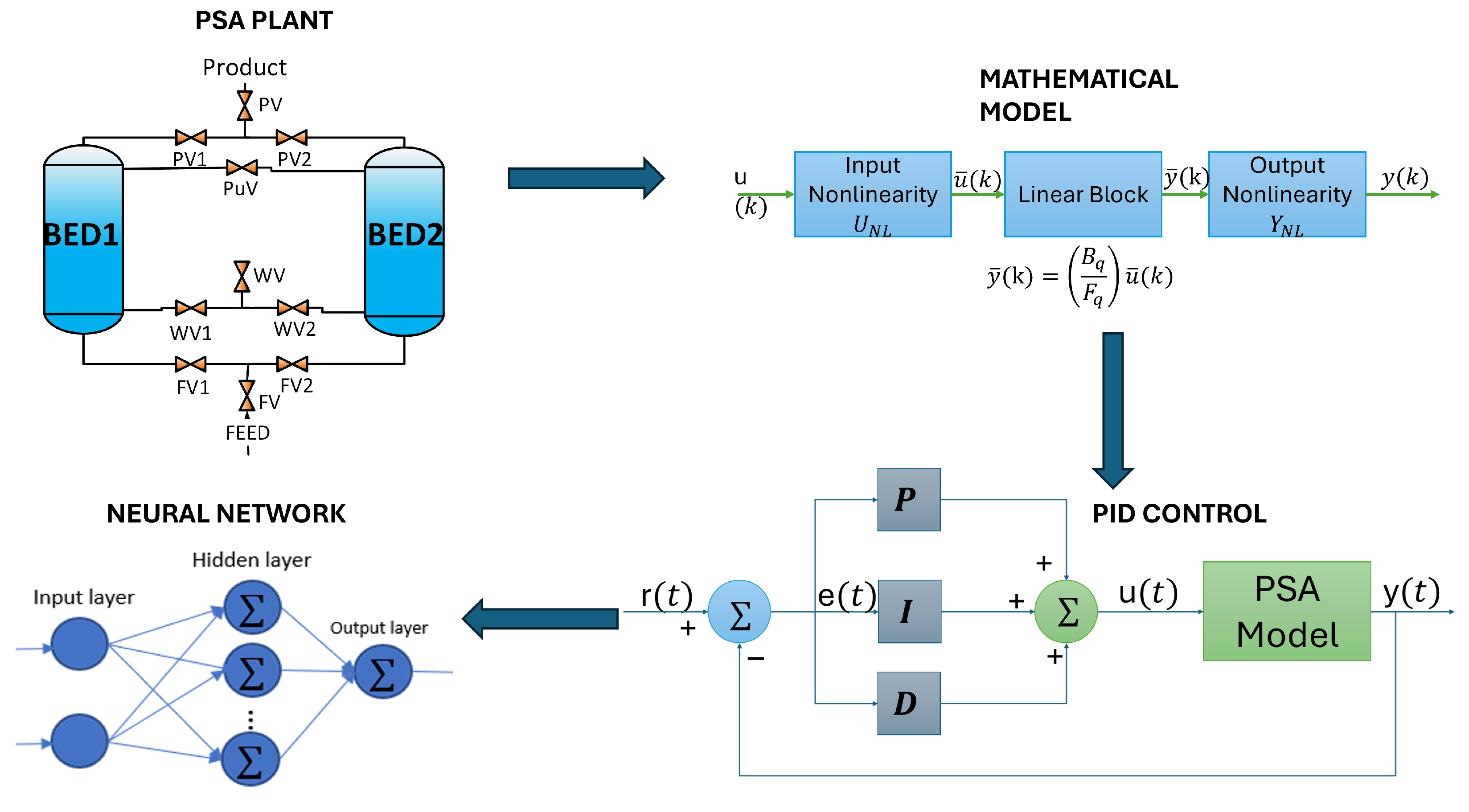
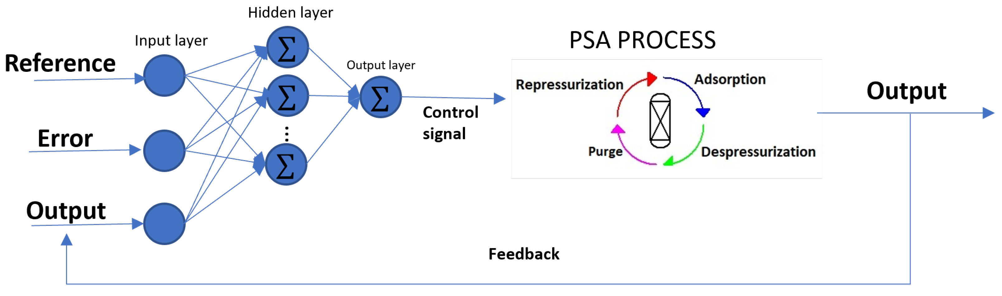
The key contribution of this article is the development of a neural network (NN) capable of effectively controlling a complex system, such as the PSA process, for biohydrogen production. The proposed method involves training and optimizing an NN model to maintain biohydrogen purity, meet international biofuel standards (exceeding 99% purity), and mitigate disturbances in the output of the PSA process. The NN was designed to emulate the behavior of a PID controller, utilizing four input–output predictors linked to the PSA process while ensuring consistent biofuel purity. The NN operates by processing reference, error, and output signals to generate control signals, which are then used to minimize disturbances and stabilize the system.

This article outlines the methodology for developing a NN to control and maintain the purity of biohydrogen. Section 2 details the simulation process used to gather the necessary data. Section 3 outlines the methodology in a step-by-step manner, beginning with the data collection and progressing through signal pre-processing, control design, the neural network (NN) learning phase, and controller analysis, ultimately leading to the control of the PSA process. Section 4 presents the results, demonstrating the ability to maintain biohydrogen purity in the presence of disturbances, and, finally, the conclusions.

2. PSA Plant Model and Simulation

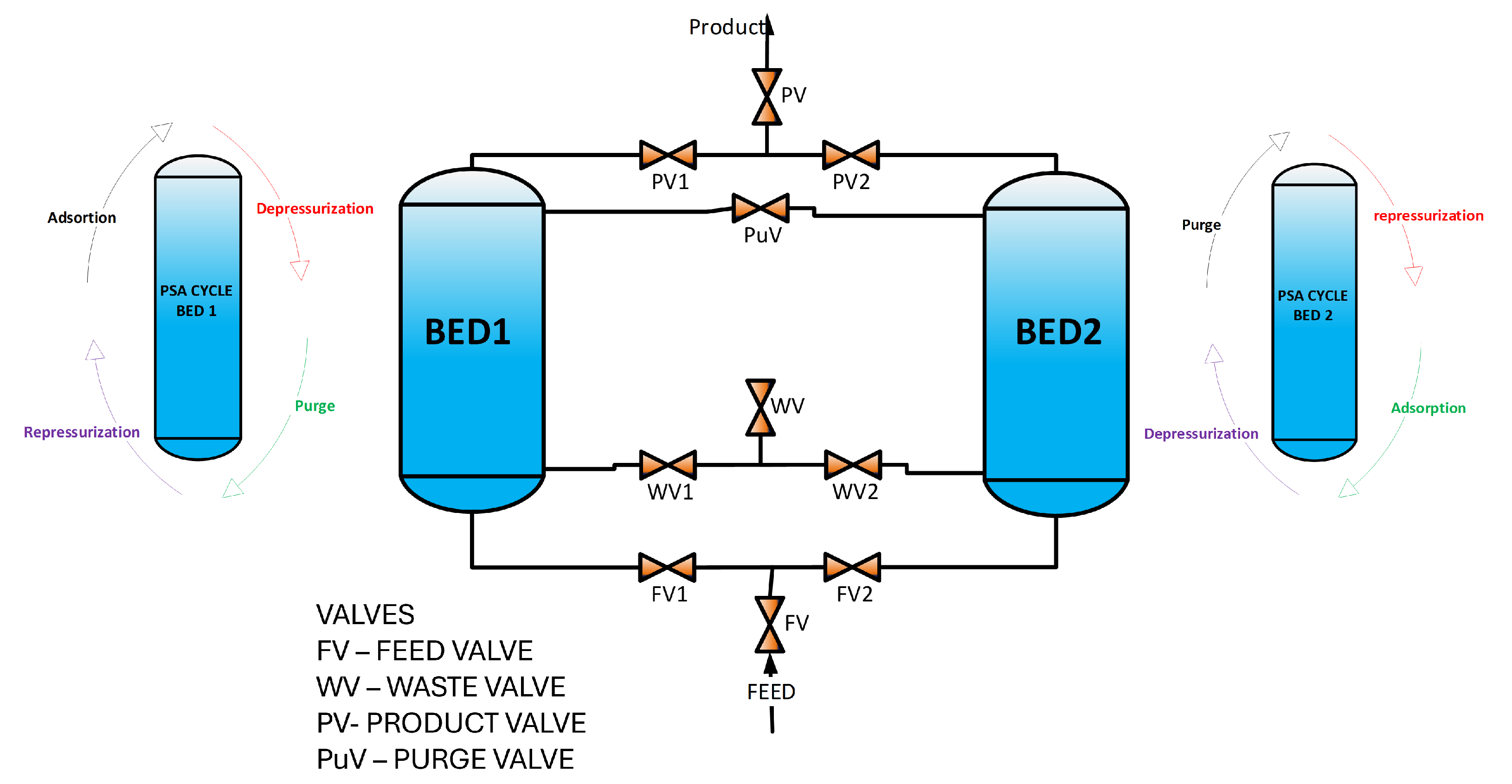
The PSA system comprises two columns interconnected by ten proportional valves (see Figure 1). The size and nominal conditions for running this plant under nominal conditions are described in

Table 1. Data required for the biohydrogen production.

Main Flows
	Feed	Product
Flow (kmol/h)	0.162	0.162
Temperature (°K)	298.15	298.15
Pressure (kPa)	100	980
H2 molar fraction	0.69	0.9485
Sizing
Bed diameter	0.037 m
Bed height	1.000 m
Zeolite type	5 A
Zeolite radius	0.0015 m
Packed density	850 kg/m3

.

The PSA plant consists of two parallel columns packed with 5A zeolite. Ten proportional valves are utilized to facilitate gas transfer between columns. Figure 1 illustrates the nominal initial parameters.

The PSA process involves a feed of the synthesized gas containing the following composition: H₂ (69%), CH₄ (28%) and CO (11%). The process consists of four steps: adsorption, depressurization, repressurization, and purge. Each stage has its own time, which makes this process cyclical until reaching the production objective.

The first step consists of feeding Bed 1 with the mixture of gases, where an adsorption step takes place for 70 s to initiate the hydrogen production. Simultaneously, Bed 2 passes through the purge step to realese the absorbent in the column.

Following that, both beds undergo the depressurization and repressurization steps for 3 s. In this step, the pressure drops or rises as follows; depressurization from 980 kPA to 150 kPa, and repressurization from 150 kPa to 980 kPa.

Then, the purge step occurred in the Bed 1 for 70 s, and the Bed 2 undergoes the adsorption process for 70 s, absorbing and retaining the compounds to purify hydrogen. The purge step carried out during the cycle performs the operation of depressurizing the beds.

Finally, repressurization and depressurization were carried out again in both beds.

In conclusion, the four steps are repeated until the operation cycle is complete. This process achieves a biohydrogen purity of 0.9485 in molar fraction.

Table 2. Process steps and times.

	Step 1		Step 2	Step 3		Step 4
Bed 1	Adsorption (70 s)	980 kPa	Despressurization (3 s)	Purge (70 s)	150 kPa	Repressurization (3 s)
Bed 2	Purge (70 s)	150 kPa	Repressurization (3 s)	Adsorption (70 s)	980 kPa	Despressurization (3 s)

summarizes the times necessary for each step and pressure.

The type 5A zeolite exhibits exceptional resistance to high temperatures and pressure fluctuations, experiencing minimal degradation compared to other adsorbents. Its adsorption capacities per gram of adsorbent are as follows: CH₄: 0.030, CO: 0.049, and N₂: 0.238, allowing the production of high-purity hydrogen. The model process used in this study is based on insights from previous work [39,40,41]. The plant model incorporates partial differential equations (PDEs) governing mass and energy balance in the gas phase, differences in pressure across the system, and kinetic models for the solid adsorbent. These PDEs are coupled with the Langmuir isotherm equations to represent the adsorption dynamics accurately. The following concerns were taken into account:

• The gas within the beds adheres to the ideal gas law.
• Variations in pressure, concentration, and temperature along the radial axis are neglected.
• The pressure drop along the axial direction is considered negligible.
• The mass transfer rate is calculated using the Linear Driving Force (LDF) model.
• The adsorption and desorption behavior of the gas is characterized using the extended Langmuir model.

The adsorbent utilized in this study is type 5A zeolite, and the mathematical model of Langmuir characterizes the adsorption isotherm.

$${\zeta }_i^{*}={\displaystyle \frac{(I{P}_1-I{P}_2{T}_s)I{P}_3{e}^{i{p}_4/T_s}{P}_i}{1+{\sum }_i\left(I{P}_3{e}^{i{p}_4/T_s}{P}_i\right)}}$$

(1)

where ${\zeta }_i^{*}$ denotes the saturation capacity for compound i, T is the temperature during adsorption, $P_i$ is the partial pressure, and $I{P}_n$ with $n=1,\dots ,4$ are the Langmuir parameters.

Material, energy, and momentum balances are fundamental in chemical and process engineering, enabling a comprehensive analysis of system behavior. The material balance represented by Equation (2), based on mass conservation, accounts for inputs, outputs, and consumption of compounds. The energy balance represented by Equation (4), grounded in the first law of thermodynamics, evaluates energy exchanges and accumulation. Additionally, the momentum balance represented by Equation (3), derived from Newton’s laws, describes fluid motion and pressure distribution within a system. Mass transfer principles further quantify the transport of species due to diffusion and convection, playing a critical role in separation processes and reaction engineering, which is represented Equation (5). These balances collectively help quantify flows, identify inefficiencies, optimize equipment performance, and enhance overall process efficiency. The set of equations used to solve the corresponding PDEs are listed below:

• Material balance

  $$-D_L{\displaystyle \frac{{\partial }^2{c}_i}{\partial z^2}}+{\displaystyle \frac{\partial \left(U_z{c}_i\right)}{\partial z}}+{\displaystyle \frac{\partial c_i}{\partial t}}+{\displaystyle \frac{(1-{ϵ}_b)}{{ϵ}_b}}J=0$$

  (2)
• Moment balance

  $$-{\displaystyle \frac{\partial P}{\partial z}}=\left({\displaystyle \frac{150\mu V_z{(1-{ϵ}_b)}^2}{4R_p^2{ϵ}_b^3}}+{\displaystyle \frac{1.75{\rho }_g(1-{ϵ}_b)}{\left(2R_p\right){ϵ}_b^3}}{v}_g^2\right)$$

  (3)
• Energy balance

  $$K_L{\displaystyle \frac{{\partial }^{2}T}{\partial z^2}}+\left[{ϵ}_{b}c{C}_{pg}+(1-{ϵ}_b){\rho }_p{C}_{ps}\right]{\displaystyle \frac{\partial T}{\partial t}}-{ϵ}_{b}c{C}_{pg}{U}_z{\displaystyle \frac{\partial T}{\partial z}}=(1-{ϵ}_b){\rho }_p\sum _{j=1}^N\Delta H_j{\displaystyle \frac{\partial n_j}{\partial t}}+{\displaystyle \frac{2h_{in}}{R_{in}}}(T_w-T)$$

  (4)
• Mass transfer

  $${\displaystyle \frac{\partial W_i}{\partial t}}=MT{C}_{si}(W_i^{*}-W_i),MT{C}_{si}={\displaystyle \frac{\Omega D_{ei}}{r_p^2}}$$

  (5)

Initial and boundary conditions must be taken into account;

Table 3. Initial and boundary conditions used in the process.

Conditions for Initialization and Boundaries:
Step I (Adsorption):
$t=0:c_{H_2}(z,0)=c_0,c_{C{H}_4}(z,0)=0,c_{C{O}_2}(z,0)=0,c_{CO}(z,0)=0$
$T(z,0)=T_0,T_w(z,0)=T_0,p(z,0)=p_0,$
${\eta }_i(z,0)={\eta }_i^{*},U_z=U_{z0}$
$z=0:-D_L{\displaystyle \frac{\partial c_i}{\partial z}}=u[c_i(0,t)-c_i(0^{+},t)],p=p_0,U_z=U_{z0}$
$-K_L{\displaystyle \frac{\partial T}{\partial z}}={ϵ}_b{C}_{p}g{U}_z[T(0^{-},t)-T(0^{+},t)]$
$z=L:-D_L{\displaystyle \frac{\partial c_i}{\partial z}}=0,U_z=0,-K_L{\displaystyle \frac{\partial T}{\partial z}}=0,{\displaystyle \frac{\partial p}{\partial z}}=0$
Step II (Depressurization):
$t=0:c_{H_2}(z,0)=c_0^{\left(I\right)},c_{CO}(z,0)=c_{CO}^{\left(I\right)},c_{C{H}_4}(z,0)=c_{C{H}_4}^{\left(I\right)},c_{C{O}_2}(z,0)=c_{C{O}_2}^{\left(I\right)}$
$T(z,0)=T^{\left(I\right)},p(z,0)=p^{\left(I\right)},{\eta }_i(z,0)={\eta }_i^{\ast \left(I\right)}$
$z=0:{\displaystyle \frac{\partial c_i}{\partial z}}=0,{\displaystyle \frac{\partial p}{\partial z}}=0$
$z=L:{\displaystyle \frac{\partial c_i}{\partial z}}=0,U_z=0,{\displaystyle \frac{\partial T}{\partial z}}=0,F=F_{\mathrm{valve}}$
Step III (Purge):
$t=0:c_{H_2}(z,0)=c_0^{\left(II\right)},c_{CO}(z,0)=c_{CO}^{\left(II\right)},c_{C{H}_4}(z,0)=c_{C{H}_4}^{\left(II\right)},c_{C{O}_2}(z,0)=c_{C{O}_2}^{\left(II\right)}$
$T(z,0)=T^{\left(II\right)},p(z,0)=p^{\left(II\right)},{\eta }_i(z,0)={\eta }_i^{\ast \left(II\right)}$
$z=0:{\displaystyle \frac{\partial c_i}{\partial z}}=0,{\displaystyle \frac{\partial p}{\partial z}}=0$
$z=L:{\displaystyle \frac{\partial c_i}{\partial z}}=0,U_z=0,{\displaystyle \frac{\partial T}{\partial z}}=0,F=F_{\mathrm{valve}}$
Step IV (Represurization):
$t=0:c_{H_2}(z,0)=c_0^{\left(III\right)},c_{CO}(z,0)=c_{CO}^{\left(III\right)},c_{C{H}_4}(z,0)=c_{C{H}_4}^{\left(III\right)},c_{C{O}_2}(z,0)=c_{C{O}_2}^{\left(III\right)}$
$T(z,0)=T^{\left(III\right)},p(z,0)=p^{\left(III\right)},{\eta }_i(z,0)={\eta }_i^{\ast \left(III\right)}$
$z=0:{\displaystyle \frac{\partial c_i}{\partial z}}=0,{\displaystyle \frac{\partial p}{\partial z}}=0$
$z=L:{\displaystyle \frac{\partial c_i}{\partial z}}=0,U_z=0,{\displaystyle \frac{\partial T}{\partial z}}=0,F=F_{\mathrm{valve}}$

summarizes them.

The energy, recovery of H₂, and the productivity of H₂ of the plant were evaluated using the following Equations (6)–(8):

$$productivit{y}_{H_2}(\%)={\displaystyle \frac{{\int }_0^{t_{Ads}}c{H}_{2}P{u}_{s}Pdt}{{\Sigma }_{i=1}^n{\int }_0^{t_{ads}}ciP{u}_{s}dt}}$$

(6)

$$Recover{y}_{H_2}(\%)={\displaystyle \frac{{\int }_0^{tAds}c{H}_{2}P{u}_{s}pdt-{\int }_0^{tPurge}c{H}_{2}P{u}_{s}Purgedt}{{\int }_0^{tAds}c{H}_{2}f{u}_{s}fdt+{\int }_0^{tARp}c{H}_{2}f{u}_{s}fdt}}$$

(7)

$$Energyefficiency(\%)={\displaystyle \frac{n_s}{n_s-1}}R{T}_{gf}\left[{\left({\displaystyle \frac{Patm}{Pva}}\right)}^{{\displaystyle \frac{n_s-1}{n_s}}}-1\right]u_{sf}{c}_{gf}\pi r^{2}bi$$

(8)

The operating conditions for the process were established based on methodologies reported by [39,40], utilizing activated carbon for hydrogen purification and production. The schematic diagram of the PSA process, illustrated in Figure 1, shows the cycles of the PSA process.

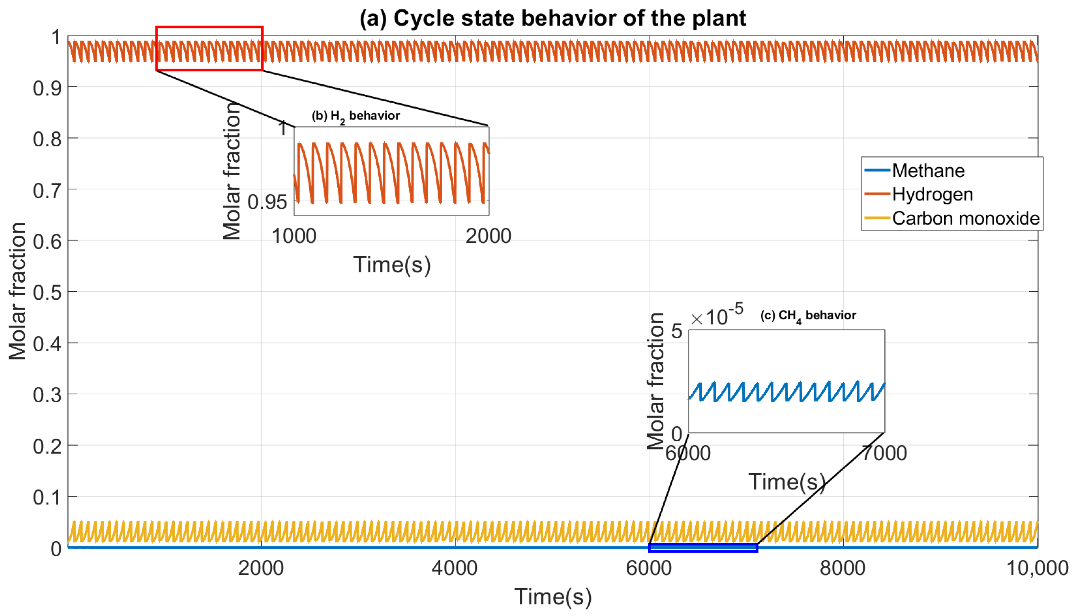
The PSA process incorporates inputs such as pressure, temperature, flow, and composition (see Figure 1). Consequently, each of the formulated equations provides a solution for these variables. Material balance allows for the determination of each component’s purity in terms of concentration or molar fraction. The momentum balance provides insights into pressure profiles within the beds, highlighting potential pressure drops that may occur during transitions between steps. The energy balance provides insight into temperature variations within the bed, which is critical to monitor since stable temperatures are essential to avoid disrupting the adsorption of molecules or atoms. The kinetic and thermodynamic model quantifies the number of adsorbed molecules and the rate at which they reach saturation. The PSA process operates under a Cyclic Steady State (CSS), and the resulting product purities are illustrated in Figure 2.

3. Methodology

We proposed a methodology for building an NN controller using the input–output signals of the PSA process and a PID control. The steps are as follows: construct a dataset from the PSA plant, identify a mathematical model using the identification systems techniques, and then create a PID control for the production of biohydrogen. After that, the signals are obtained by training the neuronal network and control the PSA plant using the NN. Figure 3 shows the method implemented in this research.

3.1. Mathematical Model

The PSA process is complex because it operates cyclically and reaches a cyclic steady state. The rigorous model is difficult to control. Our solution involves using the input and output data from the rigorous model to create a simplified model using system identification techniques [42]. The model used is a nonlinear Hammerstein-Wiener model, which consists of a linear component and two nonlinear components. The data used in this study were sourced from the work referenced in [23,43]. Figure 4a shows the identified model and Figure 4b the inverse functions.

The H-W model combines a linear dynamic model with two static nonlinear blocks at the input and output, designed to capture the rigorous PSA model’s dynamics accurately. Unlike linear models, which fail to reproduce the PSA’s dynamics correctly, the H-W model was chosen due to its capability to overcome this limitation. In the controller design, the linear dynamic model was applied in conjunction with the inverse functions of the Hammerstein and Wiener blocks, ensuring smooth integration with the detailed model (see Figure 4b). The parameters of the static nonlinear functions and their inverses are detailed in

Table 4. Parameters of the nonlinear input function.

Input Nonlinearity Breakpoints
X	49.99	50.84	51.96	53.23	54.53	55.72	56.68
Y	289.03	292.02	295.01	297.99	300.99	303.98	306.97

and

Table 5. Parameters of the nonlinear output function.

Output Nonlinearity Breakpoints
X	0.96	0.99	0.88	0.77	0.71	0.42	0.23
Y	−27.72	−22.93	35.98	70.79	105.59	140.41	175.22

, while the linear dynamic model is described in Equation (9). In Table 4 and Table 5, X and Y represent the breakpoints of the static nonlinear functions in the Hammerstein-Wiener (H-W) model. These nonlinear functions are used to model the system’s nonlinear behavior at the input and output.

$${\displaystyle \frac{\overline{y}\left(k\right)}{\overline{u}\left(k\right)}}={\displaystyle \frac{-0.3410z^{-1}+z^{-2}-0.9803z^{-3}+0.3212z^{-4}}{1-2.9300z^{-1}+2.8920z^{-2}-1.0090z^{-3}-0.1701z^{-4}+0.6690z^{-5}-0.6758z^{-6}+0.2494z^{-7}-0.01424z^{-8}-0.03958z^{-9}+0.02830z^{-10}}}$$

(9)

The inverse functions for the H-W blocks were derived using the parameters provided in Table 4 and Table 5, as shown in Equations (10) and (11). Moreover, Equation (9), which defines the transfer function, was reformulated into a discrete-time state-space representation, as depicted in Equation (12).

$${\overline{u}}_k=\left\{\begin{array}{cc}3.00u\left(k\right)+310.20,& 55.70<u\left(k\right)\le 56.60,\\ 2.30u\left(k\right)+309.10,& 54.50<u\left(k\right)\le 55.70,\\ 2.30u\left(k\right)+308.90,& 53.20<u\left(k\right)\le 54.50,\\ 2.30u\left(k\right)+307.70,& 51.90<u\left(k\right)\le 53.20,\\ 2.60u\left(k\right)+306.60,& 50.80<u\left(k\right)\le 51.90,\\ 3.50u\left(k\right)+305.20,& 49.90<u\left(k\right)\le 50.80.\end{array}\right.$$

(10)

$$y\left(k\right)=\left\{\begin{array}{cc}160.55\overline{y}\left(k\right)-182.0,\hfill & 0.97<\overline{y}\left(k\right)\le 0.99,\hfill \\ 0.01\overline{y}\left(k\right)-11.5,\hfill & 0.96<\overline{y}\left(k\right)\le 0.97,\hfill \\ -539.80\overline{y}\left(k\right)+512.0,\hfill & 0.88<\overline{y}\left(k\right)\le 0.96,\hfill \\ -302.48\overline{y}\left(k\right)+302.7,\hfill & 0.76<\overline{y}\left(k\right)\le 0.88.\hfill \end{array}\right.$$

(11)

The following state-space representation describes the discrete linear system:

$$\begin{array}{c}x(k+1)=Gx\left(k\right)+H\overline{u}\left(k\right)\\ \overline{y}\left(k\right)=Cx\left(k\right)\end{array}$$

(12)

$$G=\left[\begin{array}{cccccccccc}2.930& -1.446& 0.504& 0.085& -0.334& 0.337& -0.124& 0.007& 0.039& -0.113\\ 2& 0& 0& 0& 0& 0& 0& 0& 0& 0\\ 0& 1& 0& 0& 0& 0& 0& 0& 0& 0\\ 0& 0& 1& 0& 0& 0& 0& 0& 0& 0\\ 0& 0& 0& 1& 0& 0& 0& 0& 0& 0\\ 0& 0& 0& 0& 1& 0& 0& 0& 0& 0\\ 0& 0& 0& 0& 0& 1& 0& 0& 0& 0\\ 0& 0& 0& 0& 0& 0& 1& 0& 0& 0\\ 0& 0& 0& 0& 0& 0& 0& 0.500& 0& 0\\ 0& 0& 0& 0& 0& 0& 0& 0& 0.250& 0\end{array}\right],$$

$$H={\left[\begin{array}{cccccccccc}1& 0& 0& 0& 0& 0& 0& 0& 0& 0\end{array}\right]}^T,$$

$$C=\left[\begin{array}{cccccccccc}-0.34& 0.50& -0.49& 0.16& 0& 0& 0& 0& 0& 0\end{array}\right],$$

Let $\mathbf{x}\in {\mathbb{R}}^{n\times 1}$ represent the state vector, $\overline{\mathbf{u}}\in {\mathbb{R}}^{m\times 1}$ represent the input vector, and $\overline{\mathbf{y}}\in {\mathbb{R}}^{r\times 1}$ represent the output vector. Consequently, let $\mathbf{G}\in {\mathbb{R}}^{n\times n}$ denote the state matrix, $\mathbf{H}\in {\mathbb{R}}^{n\times m}$ denote the input matrix, and $\mathbf{C}\in {\mathbb{R}}^{n\times r}$ denote the output matrix. In this representation, the sampling period k is assumed to be 1 s.

3.2. Design of PID Discrete Controller

This section covers the development of a discrete PID controller to control the purity of the biohydrogen and the temperature of the reboiler at the beds.

The control law for the discrete PID is given by:

$$u\left(k\right)=K_pϵ\left(k\right)+K_i\sum _{i=0}^kϵ\left(k\right)\Delta t+K_d{\displaystyle \frac{ϵ\left(k\right)-ϵ(k-1)}{\Delta t}}$$

(13)

where $ϵ\left(k\right)$ is the error at step k, $\Delta t$ is the sampling period, and $K_p,K_i,K_d$ are the proportional, integral, and derivative gains.

The gains are $K_p=-0.00781971054640794$, $K_i=-0.0156394210928159$, and $K_d=0$. In this case, the derivative gain is not used. The Ziegler–Nichols approach was employed to obtain these gains.

Figure 5 shows the behavior of the discrete PID controller using the gains $K_p,K_i,$ and $K_d$ mentioned before.

3.3. Neuronal Network

This section shows the development of the neural network, which was designed to control the biohydrogen purity in the PSA plant. We used the reference, the output, and the error as the NN’s inputs and the signal generated by the PID controller as the output/target. Figure 6 presents a compelling illustration of the operation of the NN-based PID controller within the system.

The NN represented in Figure 6 can be expressed as:

$$z_m=\sum _{k=1}^K{s}_{pk}\phi \left(\sum _{j=1}^J{v}_{kj}\phi \left(\sum _{i=1}^N{w}_{ji}{x}_i+b_j\right)+b_k\right)+b_p$$

(14)

where $z_m$ is the output of the neural network, $s_{pk}$ are the weights of the output layer connecting the k-th hidden neuron to the p-th output neuron, $v_{kj}$ are the weights of the hidden layer connecting the j-th input neuron to the k-th hidden neuron, $w_{ji}$ are the weights of the input layer connecting the i-th input feature to the j-th hidden neuron, $x_i$ are the inputs to the neural network, $b_j$ is the bias for the j-th hidden neuron, $b_k$ is the bias for the k-th hidden neuron, $b_p$ is the bias for the p-th output neuron, and $\phi (.)$ is the activation function. Algorithm 1 describes all the steps needed to get the neural network to work as a controller.

In this neural network (NN), three input signals—reference, error, and output values—are used along with one target signal to approximate the control signal. As presented in Figure 7, the signals employed for training are the reference and output values. Figure 8 demonstrates the trained NN results, achieving a fit of 98.64% and an error of 0.054 using the Root Mean Square Error (RMSE) formula.

Algorithm 1 Algorithm for Building a Neural Network Model for PID Control

Input: Reference signal, error signal $ϵ\left(k\right)$, Output signal $y\left(k\right)$ Output: Action Control signal $u\left(k\right)$        Initialization;   1: Gather data from the plant and the PID.   2: Train the neural network (NN) using the Adam optimization algorithm.   3: while $\mathrm{RMSE}\le 0.99$ do   4:     Identify the optimal number of hidden layers for the neural network.   5:     Select the appropriate number of input and hidden layers neurons.   6:     Specify the activation functions to be used in each layer of the network.   7:     Train the NN using the Adam algorithm.   8:     Evaluate the model’s accuracy using standardized metrics, including MSE, MAE, and NRMSE.   9: end while

The following key factors play a crucial role in supporting the stability of our neural network model:

• The data set obtained from the PSA plant consists of approximately 350,000 data points, divided into 50% for training, 25% for validation, and 25% for testing. The use of a large and diverse dataset contributes significantly to the stability of the model.
• The Adam optimizer algorithm, widely recognized for its efficiency in machine learning, is used to train the neural network. Its primary objective is to iteratively approximate the parameters toward an optimal solution by resolving a quadratic function in small incremental steps. Although convergence may take time, the gradient-based approach ensures stability in the algorithm.
• Due to its ability to reduce the vanishing gradient problem, the Rectified Linear Unit (ReLU) activation function is preferred in deep networks. By maintaining stronger gradients during backpropagation, ReLU enhances the stability and performance of the network.
• The small gain theorem [44] is applied to guarantee uniform stability and ultimate boundedness. Using the weights of the NN, the result is calculated as:

  $${\gamma }_{sg}={\displaystyle \frac{1}{1-∥W∥}},$$

  (15)

  yielding a value of 0.0072.

Additionally, disturbances are introduced to the system’s output to assess its stability. The results of these tests are presented and discussed in detail in the results section.

Table 6. Key parameters of the feedforward multi-layer neural network.

Component	Specification	Assigned Value
Input Layer	Number of input features	8 (4 from feedback signals, 4 as reference inputs)
Hidden Layers	Total hidden layers	1
Neurons per Layer	Distribution across layers	8 (Input), 64 (Hidden), 1 (Output)
Output Layer	Neurons in the output layer	1
Activation Functions	Applied activation per layer	ReLU (Input Layer), ReLU (Hidden Layer), None (Output Layer)
Optimization Method	Algorithm used for optimization	Adam
Training Epochs	Total number of epochs	100
Network Type	Learning approach	Regression Model
Loss Function	Error function used	Mean Squared Error (MSE)
Evaluation Metrics	Performance metrics used	Mean Absolute Error (MAE), Mean Squared Error (MSE)
Validation Split	Data reserved for validation	25%

summarizes the parameters of a feedforward multi-layer neural network designed for regression tasks. It consists of an input layer with eight features (4 from feedback and 4 for reference), one hidden layer with 64 neurons, and a single output neuron. The ReLU activation function is applied in the input and hidden layers, while the output layer has no activation. The Adam optimizer is used for training over 100 epochs. This configuration suggests a simple yet efficient architecture aimed at learning complex relationships in the data while maintaining computational efficiency.

Figure 9 presents the training curves of the neural network (NN) controller. Part (a) shows the behavior of the loss metric for the training and validation data, plotted over 50 training epochs of the model. Part (b) shows the Mean Squared Error (MSE) curve over these 50 epochs. The result is a reliable model that was not overtrained.

4. Results

This study explores the use of neuronal networks to mimic the behavior of a PID controller in regulating biohydrogen purity. In this context, three main signals are involved in the training process:

• The feedback signal represents the purity of the biohydrogen, enabling dynamic adjustments in control actions to maintain the desired performance.
• The error signal is computed as the difference between the reference signal and the feedback signal.
• The reference signal corresponds to the desired purity level of the biohydrogen.

The NN architecture comprises three layers: an input layer with eight neurons using a ReLU activation function, a hidden layer with 64 neurons and ReLU activation, and an output layer without activation function. The NN is trained to map these input signals to the control actions generated by the PID controller.

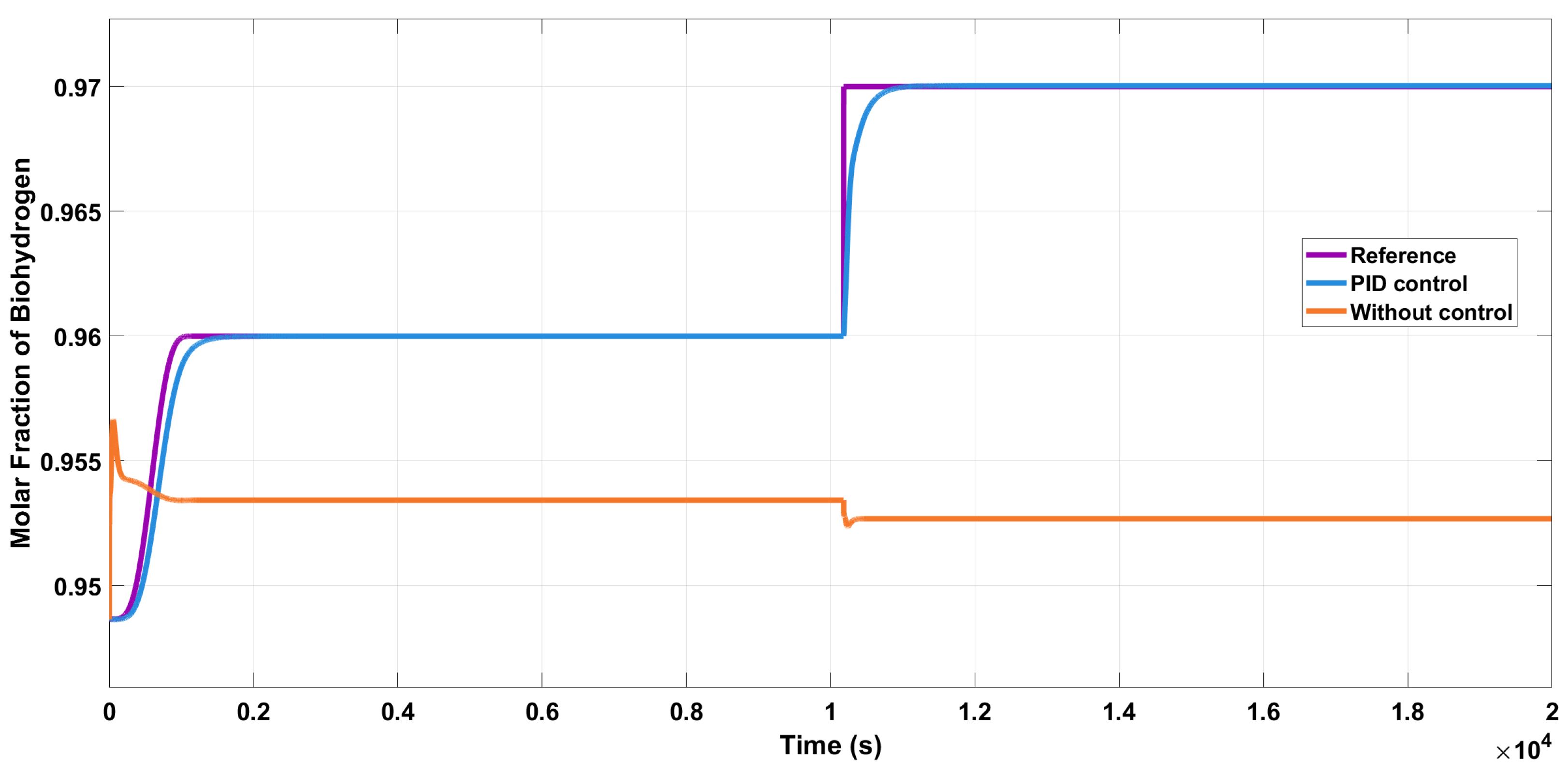
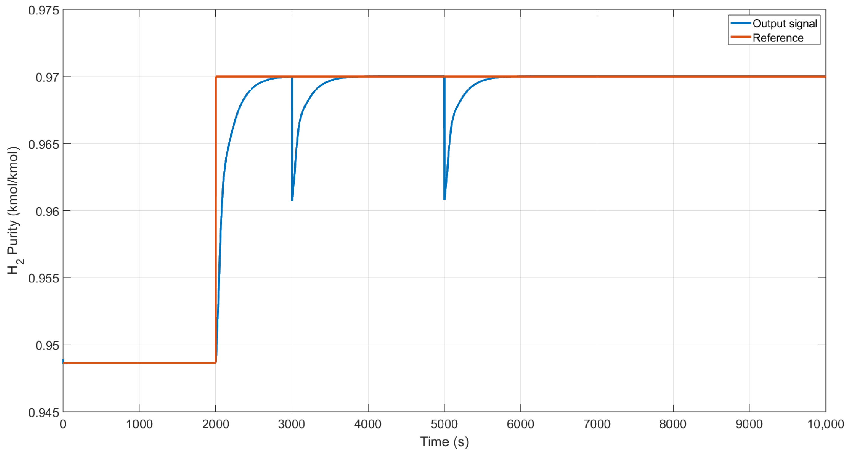
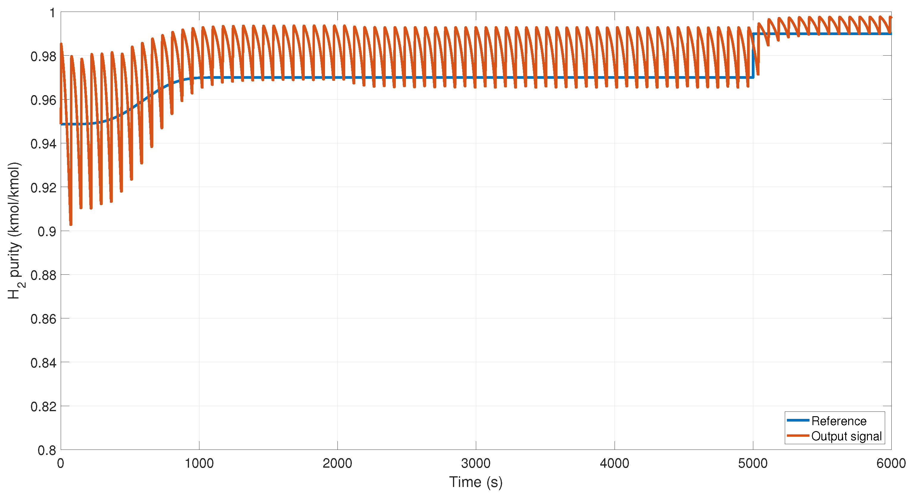
We changed the reference from 0.94 to 0.97 kmol/kmol of H₂ and added additive perturbations at the output of the system, as shown in Figure 10. The controller reacts slowly due to the type of process; however, it reaches the reference despite the perturbations.

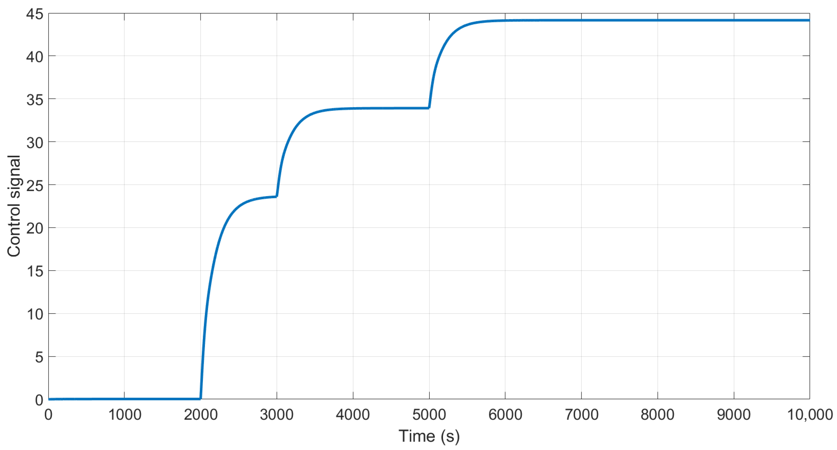
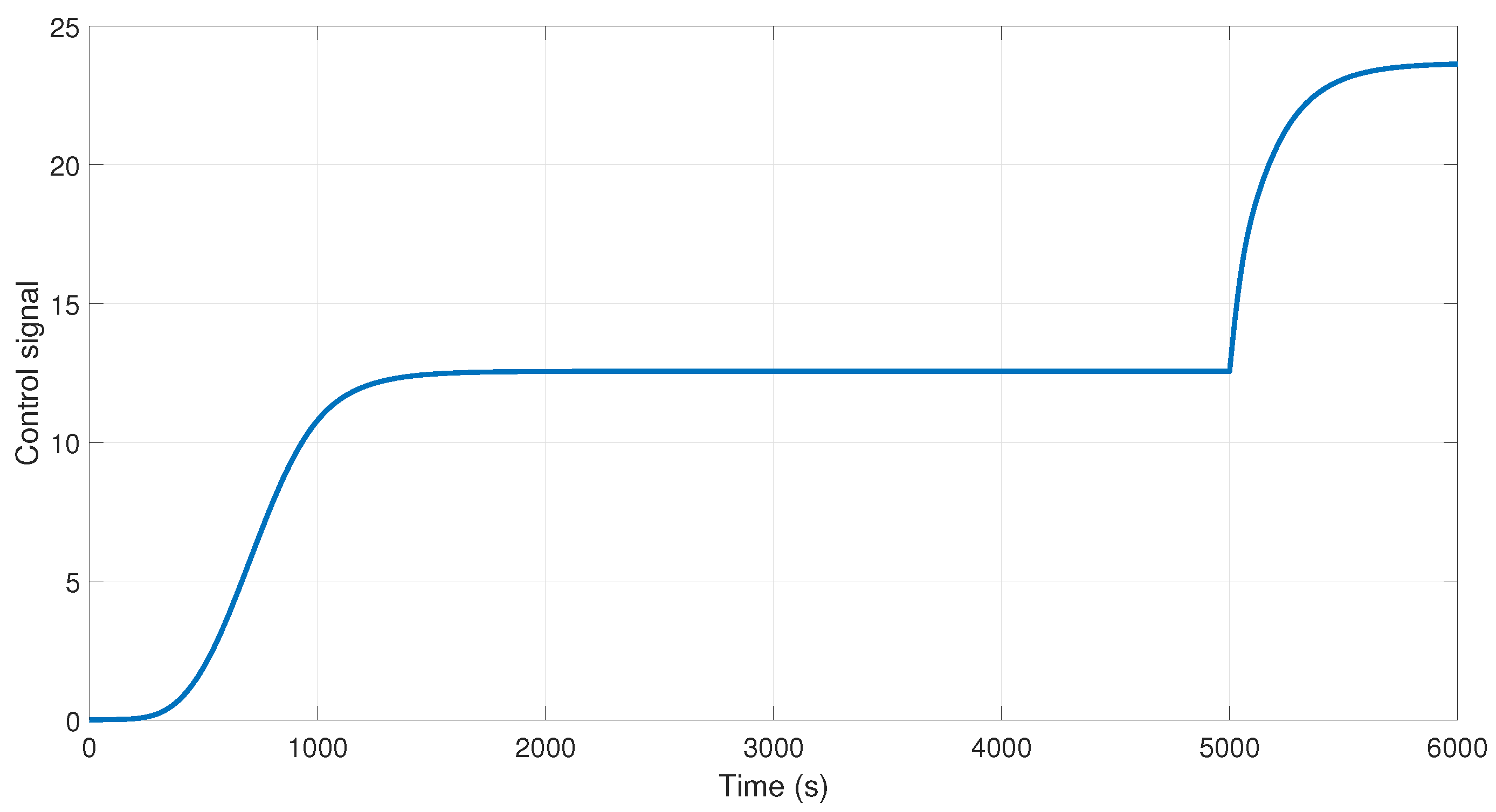
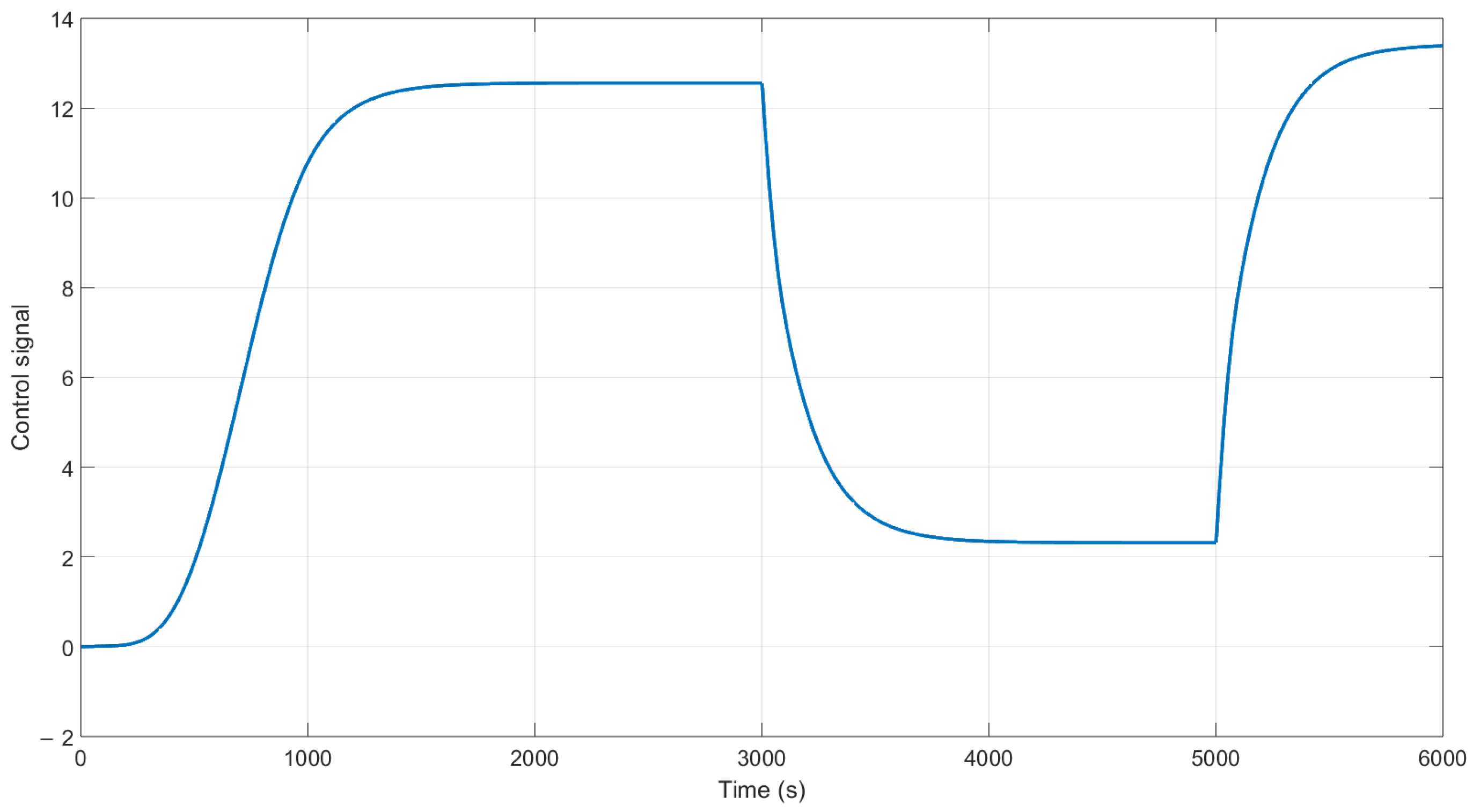
The behavior of the control signal is presented in Figure 11. We can observe that in the time 3000 and 5000 s, the control increases the action of control to maintain the output at the desired purity using the H-W model.

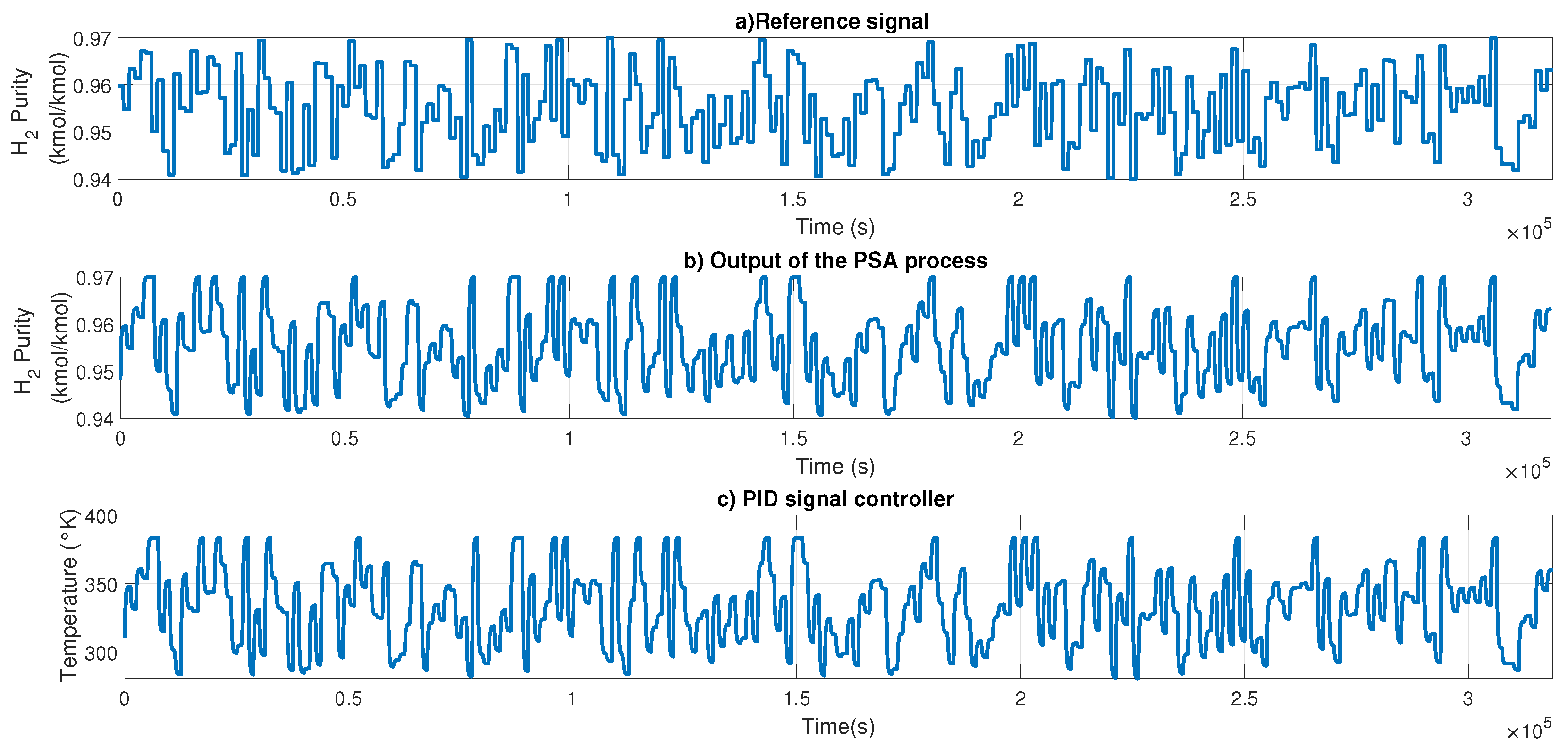
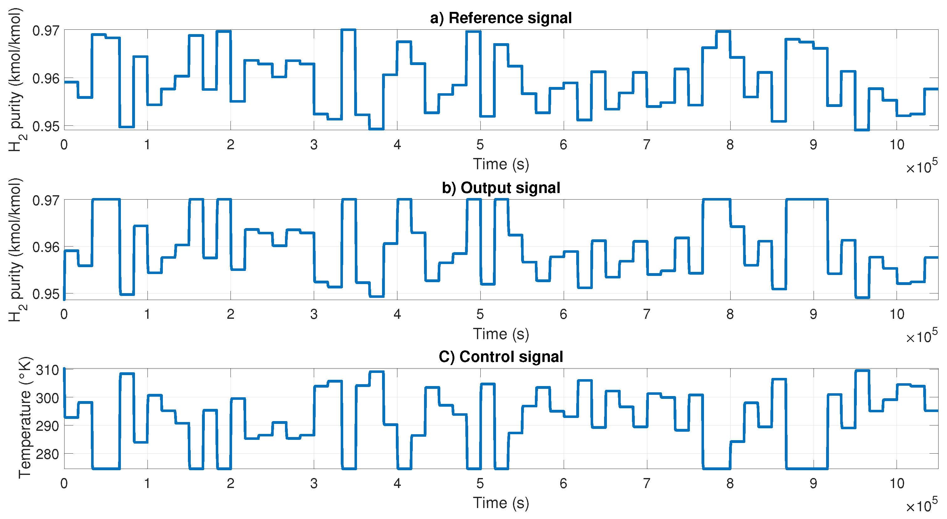
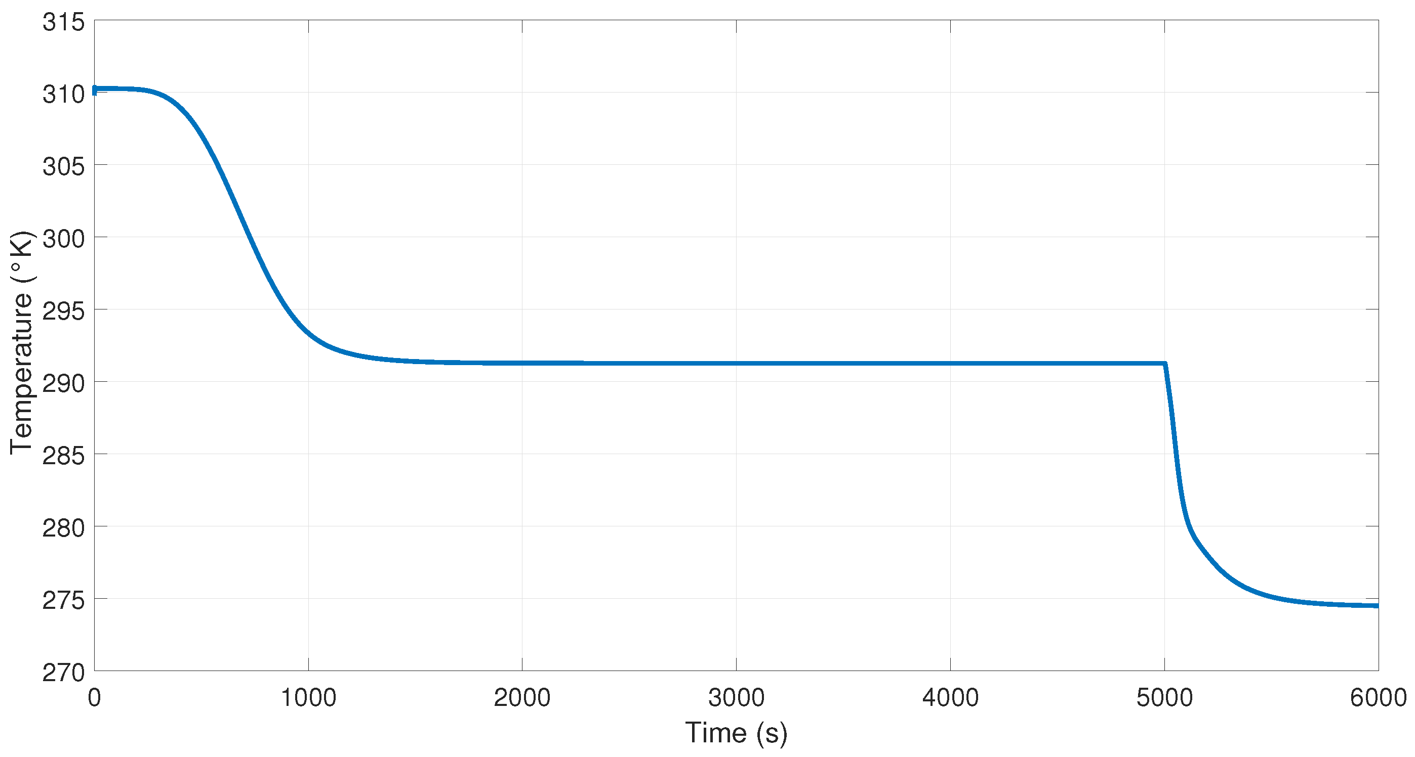
The NN controller was tested using a 6-bit PRBS signal with variable amplitude as input. The results are shown in Figure 11; in Figure 12a, the PRBS signal is presented; Figure 12b shows the output of the H-W model to perform the feedback; Figure 12c shows the controller signal generated by PID to control the purity using the temperature of the reboiler.

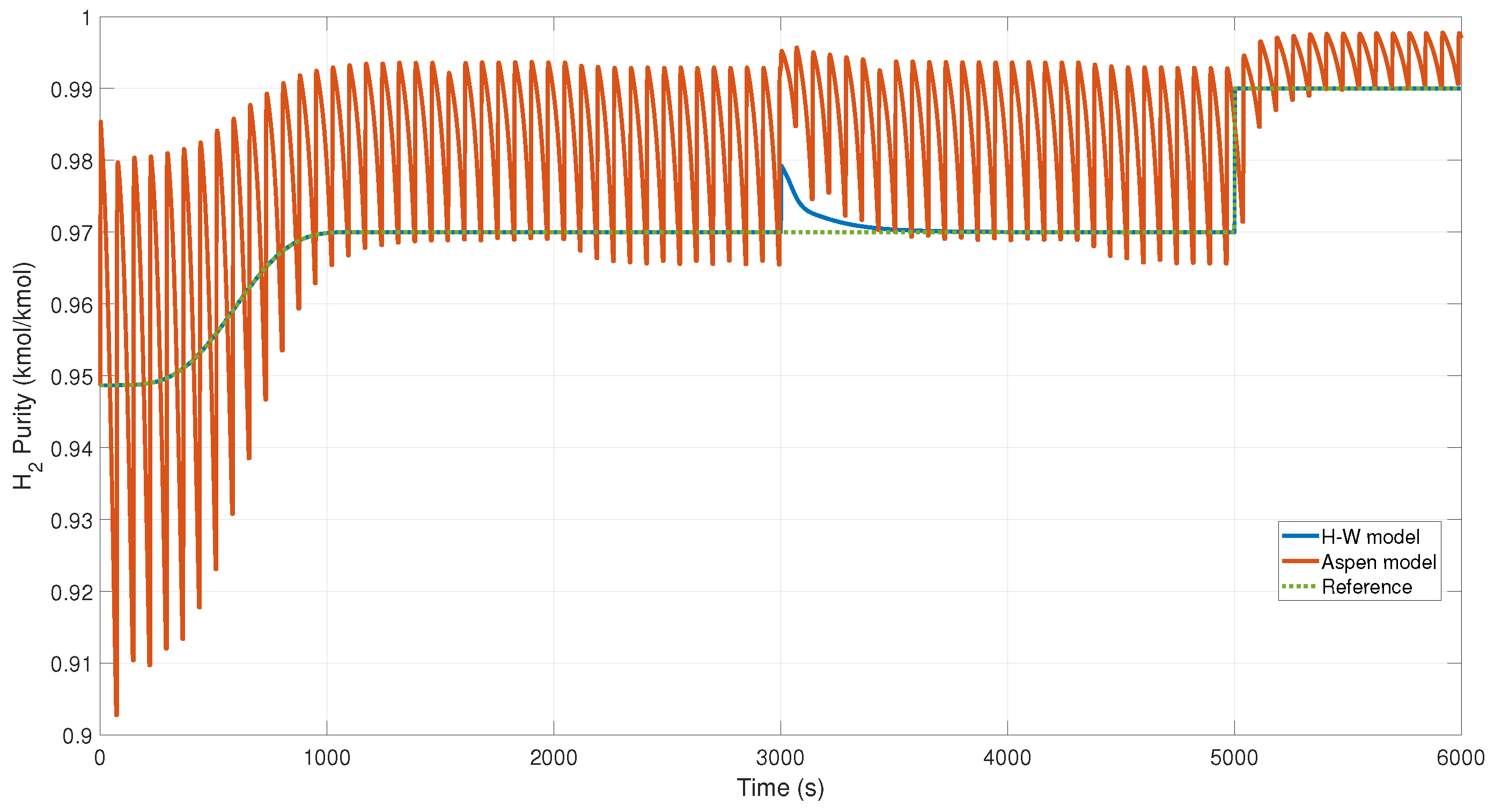
We used the PSA plant simulated in Aspen Adsorption to validate our controller because this tool allows accurate simulations and detailed analysis of adsorption processes. Figure 13 shows the behavior of the purity of the biohydrogen using the NN controller when two reference changes were applied—one at 1000 s from 0.94 to 0.97 and the other from 0.97 to 0.99 at 5000 s.

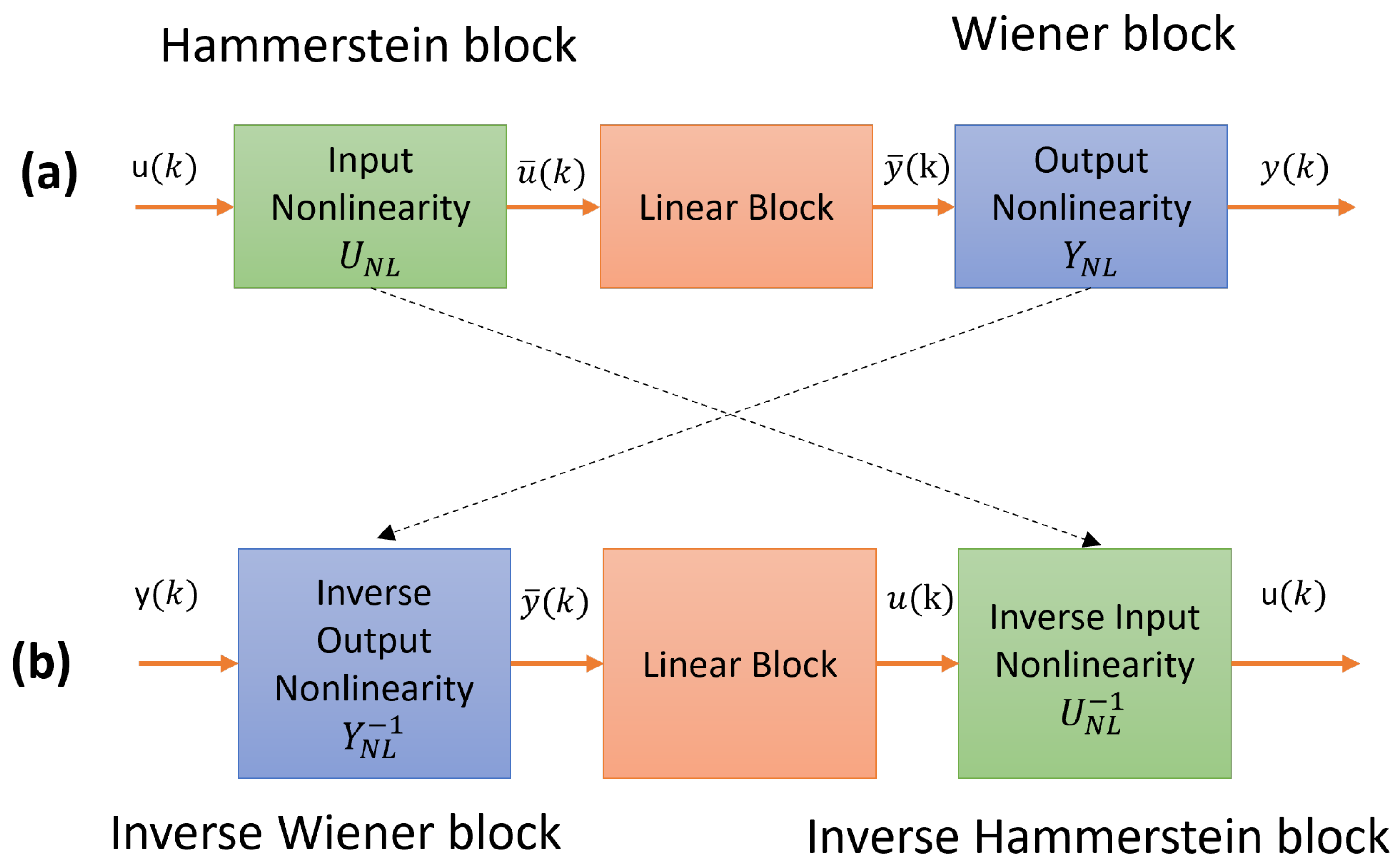
Figure 14 shows the control signal of the NN controller; in this case, it is the output for the linear model. However, by using the inverse equations calculated in the mathematical model section, which are Equations (10) and (11), we obtain the control signal for the production of biohydrogen using the PSA plant simulated in Aspen; this signal is shown in Figure 15.

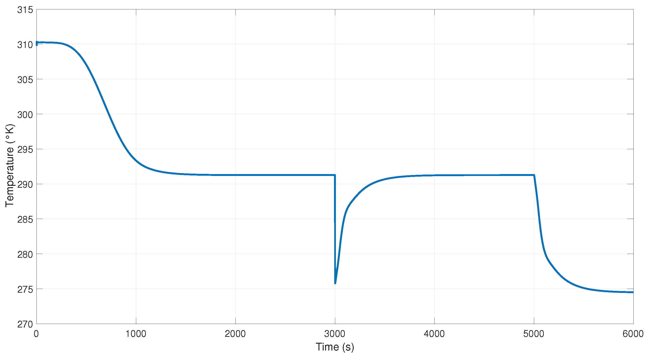
Figure 16 shows the behavior of the NN controller at the Aspen model and the H-W model when a disturbance occurred at time 3000 s in the output of the system. We can observe an overshoot at this time because of the disturbance applied.

Figure 17 presents the NN controller’s performance in response to a disturbance at 3000 s in the output of the system; remember that first the NN controller is applied without the inverse blocks. The temperature to control the heat in the reboiler to maintain purity when using the inverse blocks is presented in Figure 18. In this figure, we can see the disturbance that occurs at 3000 s, but the purity of the product is not affected, maintaining the margin; this is because the controller sends a signal that keeps it cyclically stable in the reference (see Figure 16).

Furthermore,

Table A1. Flow report at the 10th cycle.

	Value	Units	Description
Total_Material_Fwd	0.530924	kmol	Total material received at boundary
Total_Component_Fwd (*)
Total_Component_Fwd (“CO”)	0.0820483	kmol	Total component received at boundary
Total_Component_Fwd (“HYDROGEN”)	0.220483	kmol	Total component received at boundary
Total_Component_Fwd (“METHANE”)	0.228392	kmol	Total component received at boundary
Avg_Composition_Fwd (*)
Avg_Composition_Fwd (“CO”)	0.154539	kmol/kmol	Average composition received at boundary
Avg_Composition_Fwd (“HYDROGEN”)	0.415282	kmol/kmol	Average composition received at boundary
Avg_Composition_Fwd (“METHANE”)	0.430179	kmol/kmol	Average composition received at boundary
Total_Energy_Fwd	−26.2464	MJ	Total energy received at boundary
Total_Material_Rev	0.00647435	kmol	Total material fed at boundary
Total_Component_Rev (*)
Total_Component_Rev (“CO”)	0.00215812	kmol	Total component fed at boundary
Total_Component_Rev (“HYDROGEN”)	0.00215812	kmol	Total component fed at boundary
Total_Component_Rev (“METHANE”)	0.00215812	kmol	Total component fed at boundary
Avg_Composition_Rev (*)
Avg_Composition_Rev (“CO”)	0.333333	kmol/kmol	Average composition fed at boundary
Avg_Composition_Rev (“HYDROGEN”)	0.333333	kmol/kmol	Average composition fed at boundary
Avg_Composition_Rev (“METHANE”)	0.333333	kmol/kmol	Average composition fed at boundary
Total_Energy_Rev	−0.399401	MJ	Total energy fed at boundary
Cycle_Total_Material_Fwd	0.00570575	kmol	Total received at boundary over last cycle
Cycle_Total_Component_Fwd (*)
Cycle_Total_Component_Fwd (“CO”)	9.93 × ${10}^{-4}$	kmol	Total component received at boundary over last cycle
Cycle_Total_Component_Fwd (“HYDROGEN”)	0.00239531	kmol	Total component received at boundary over last cycle
Cycle_Total_Component_Fwd (“METHANE”)	0.00231734	kmol	Total component received at boundary over last cycle
Cycle_Avg_Composition_Fwd (*)
Cycle_Avg_Composition_Fwd (“CO”)	0.174053	kmol/kmol	Average composition received at boundary over last cycle
Cycle_Avg_Composition_Fwd (“HYDROGEN”)	0.419806	kmol/kmol	Average composition received at boundary over last cycle
Cycle_Avg_Composition_Fwd (“METHANE”)	0.406141	kmol/kmol	Average composition received at boundary over last cycle
Cycle_Total_Energy_Fwd	−0.287609	MJ	Total energy received at boundary over last cycle
Cycle_Total_Material_Rev	7.23 × ${10}^{-4}$	kmol	Total fed at boundary over last cycle
Cycle_Total_Component_Rev (*)
Cycle_Total_Component_Rev (“CO”)	2.41 × ${10}^{-4}$	kmol	Total component fed at boundary over last cycle
Cycle_Total_Component_Rev (“HYDROGEN”)	2.41 × ${10}^{-4}$	kmol	Total component fed at boundary over last cycle
Cycle_Total_Component_Rev (“METHANE”)	2.41 × ${10}^{-4}$	kmol	Total component fed at boundary over last cycle
Cycle_Avg_Composition_Rev (*)
Cycle_Avg_Composition_Rev (“CO”)	0.333333	kmol/kmol	Average composition fed at boundary over last cycle
Cycle_Avg_Composition_Rev (“HYDROGEN”)	0.333333	kmol/kmol	Average composition fed at boundary over last cycle
Cycle_Avg_Composition_Rev (“METHANE”)	0.333333	kmol/kmol	Average composition fed at boundary over last cycle
Cycle_Total_Energy_Rev	−0.0445976	MJ	Total energy fed at boundary over last cycle

presents an analysis of the flows and energy consumed in the adsorption process in the 44th cycle. Also,

Table 7. Productivity report at the highest purity (0.99 kmol/kmol) in the 35th cycle.

Stream	Unit	FV	WV	PV	BED1	BED2
Total material forward	kmol	0.00757	0.00481	0.00247	0.00185	6.14 × ${10}^{-4}$
Average flowrate forward	kmol/s	5.19 × ${10}^{-5}$	3.30 × ${10}^{-5}$	1.69 × ${10}^{-5}$	1.27 × ${10}^{-5}$	4.21 × ${10}^{-6}$
Total Component Forward
CO	kmol	8.33 × ${10}^{-4}$	7.61 × ${10}^{-4}$	3.12 × ${10}^{-5}$	2.95 × ${10}^{-5}$	9.78 × ${10}^{-6}$
HYDROGEN	kmol	0.00462	0.00207	0.00244	0.00182	6.05 × ${10}^{-4}$
METHANE	kmol	0.00212	0.00198	3.64 × ${10}^{-8}$	2.93 × ${10}^{-8}$	9.72 × ${10}^{-9}$
Average Composition Forward
CO	kmol/kmol	0.11	0.158	0.013	0.016	0.016
HYDROGEN	kmol/kmol	0.61	0.43	0.987	0.984	0.984
METHANE	kmol/kmol	0.28	0.412	1.48 × ${10}^{-5}$	1.58 × ${10}^{-5}$	1.58 × ${10}^{-5}$
Energy Consumption
Total energy forward	MJ	0.2531	0.2345	0.0042	0.0037	0.0012
Average enthalpy forward	MJ/kmol	33.42	48.72	1.71	1.98	1.97
Total energy reverse	MJ	0.0	0.0058	0.0	9.20 × ${10}^{-4}$	8.98 × ${10}^{-4}$
Average enthalpy reverse	MJ/kmol	0.0	61.69	0.0	1.49	1.46

shows the productivity report for the 35th cycle. Analyzing the table, we concluded that we had an efficient separation process with minimal reverse flow. In addition, we obtained high hydrogen purity, about 0.99 kmol/kmol, in most of the streams. Carbon monoxide maintains a steady presence at around 11%, while methane remains at about 28%, with negligible reverse amounts. The total forward material is consistently distributed across the different streams, ensuring a smooth process operation.

The energy efficiency and recovery of H₂ are reported in

Table 8. Energy efficiency and recovery H₂ report.

Product:	PV (%)	WV (%)
Material:	32.5695	63.5582
Component:
CO	3.73975	91.3675
HYDROGEN	61.7174	44.8093
METHANE	0.0017184	93.4792
Energy	1.67027	92.6473

where we can find that most of the energy is held in the waste stream. The system successfully removes impurities.

Table 7 shows the productivity achieved in each section of the process using NN control. Significant results are observed since the productivity is higher than that obtained in the open loop (without control), generating a productivity of 0.0024 kmol and $6.14333\times {10}^{-4}$ kmol/s.

Table 8 shows the results of energy recovery and efficiency. Biohydrogen recovery is above 50% using NN control, generating an energy efficiency of 1.67%. These results have great scientific contribution since little energy is used to reach a purity of 99% with less energy and greater recovery. In addition, it mitigates the disturbances that exist in this complex technology.

5. Conclusions

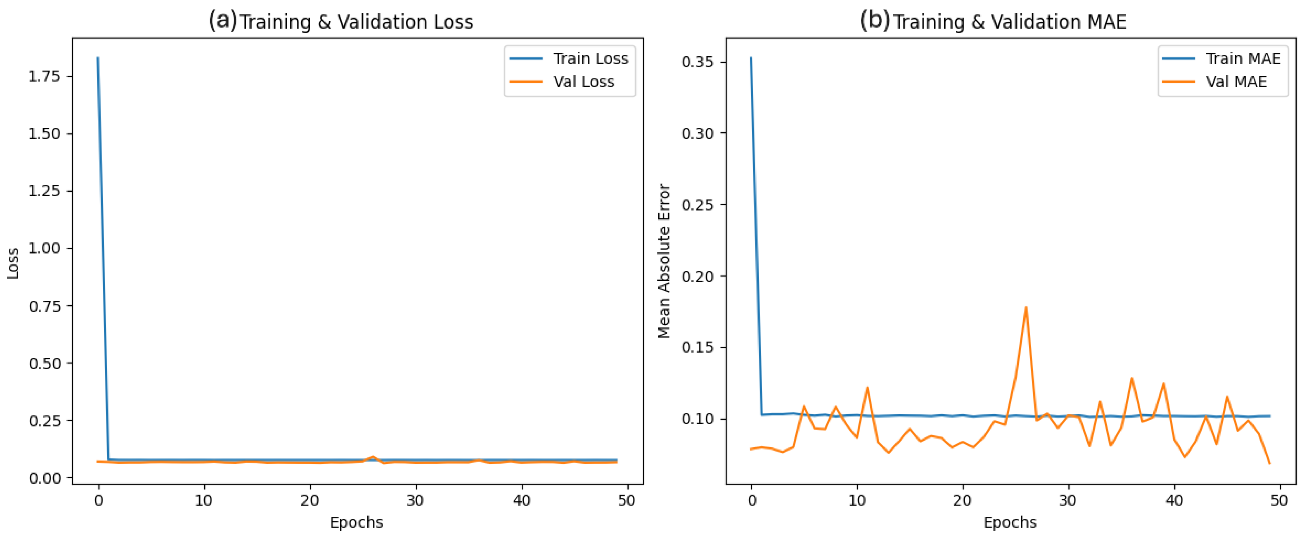
In conclusion, this study demonstrates the effectiveness of a neural PID controller in regulating product purity in the PSA process. We successfully captured the smoothed process dynamics with a 74% fit by first developing a Hammerstein-Wiener model. Using this model, a discrete PID controller was designed, and subsequently, a neural PID controller was trained to emulate its behavior. The neural PID controller was optimized using the Adam algorithm, achieving a fit of 96%.

To validate the approach, we applied system identification techniques to develop an initial model from PSA process data. The results demonstrate that the neural PID controller effectively represents the discrete PID controller, as both maintain a biohydrogen purity of 0.99 molar fraction while attenuating output disturbances.

A key finding is the high hydrogen purity (≈99%) reach in the product; this control also keeps an efficient gas separation. The analysis of the streams indicates that the methane is almost retained in the waste stream (93.48%), ensuring the purity of the H₂ in the final product.

In conclusion, the neural controller based on a discrete PID demonstrates performance and robustness equivalent to that of the discrete PID controller. Both controllers achieve the international standard for biohydrogen purity at 0.99 molar fraction while effectively countering disturbances. The advantages of using a neural network are the feasibility, adaptation to new control points, better disturbance rejection, and multivariate control. This study uses NN as a MISO (Multiple-Inputs, Single-Output) controller. In the case study, the complex behavior of the PSA plant can be challenging to control without the help of modern tools such as NN. Thus, the NN implemented in this process allows us to operate and control the desired purity despite its cyclical behavior.

Future works should focus on improving hydrogen recovery by minimizing losses in the wind-generated current stream while improving energy efficiency. Implementing energy recovery strategies could reduce waste and optimize process sustainability, ensuring better utilization of resources and increased overall system performance.

References

1. Demirbas, A. Biofuels from Agricultural Biomass. Energy Sources Part A Recover. Util. Environ. Eff. 2009, 31, 1573–1582. [Google Scholar] [CrossRef]
2. Bianco, E.; Blanco, H. Green Hydrogen: A Guide to Policy Making; IGEM: Derby, UK, 2020. [Google Scholar]
3. Boodhun, B.S.F.; Mudhoo, A.; Kumar, G.; Kim, S.H.; Lin, C.Y. Research perspectives on constraints, prospects and opportunities in biohydrogen production. Int. J. Hydrogen Energy 2017, 42, 27471–27481. [Google Scholar] [CrossRef]
4. Valdez-Resendiz, J.E.; Rumbo-Morales, J.Y.; Sorcia-Vázquez, F.D.; Ortiz-Torres, G.; Gómez-Aguilar, J.; Cantero, C.A.T.; Ramos-Martinez, M. Optimization and discrete fractional-order PID controller applied to a pressure swing adsorption plant for the production and recovery of bioethanol. J. Clean. Prod. 2024, 476, 143618. [Google Scholar] [CrossRef]
5. Rumbo-Morales, J.Y.; Ortiz-Torres, G.; Sorcia-Vázquez, F.D.; Torres-Cantero, C.A.; Radilla, J.G.; García, M.M.; Rodríguez-Cerda, J.C.; Rosales, A.M.; Ramos-Martinez, M.; Mixteco-Sánchez, J.C.; et al. Energy efficiency and productivity of a Pressure Swing Adsorption plant to purify bioethanol: Disturbance attenuation through geometric control. Digit. Chem. Eng. 2025, 14, 100209. [Google Scholar] [CrossRef]
6. Gupta, S.; Fernandes, A.; Lopes, A.; Grasa, L.; Salafranca, J. Photo-Fermentative Bacteria Used for Hydrogen Production. Appl. Sci. 2024, 14, 1191. [Google Scholar] [CrossRef]
7. Khetkorn, W.; Rastogi, R.P.; Incharoensakdi, A.; Lindblad, P.; Madamwar, D.; Pandey, A.; Larroche, C. Microalgal hydrogen production—A review. Bioresour. Technol. 2017, 243, 1194–1206. [Google Scholar] [CrossRef] [PubMed]
8. Kumar, G.; Sivagurunathan, P.; Pugazhendhi, A.; Thi, N.B.D.; Zhen, G.; Chandrasekhar, K.; Kadier, A. A comprehensive overview on light independent fermentative hydrogen production from wastewater feedstock and possible integrative options. Energy Convers. Manag. 2017, 141, 390–402. [Google Scholar] [CrossRef]
9. Show, K.Y.; Yan, Y.G.; Lee, D.J. Biohydrogen production from algae: Perspectives, challenges, and prospects. In Biofuels from Algae; Elsevier: Amsterdam, The Netherlands, 2019; pp. 325–343. [Google Scholar]
10. Logan, B.E.; Rossi, R.; Ragab, A.; Saikaly, P.E. Electroactive microorganisms in bioelectrochemical systems. Nat. Rev. Microbiol. 2019, 17, 307–319. [Google Scholar] [CrossRef]
11. Baeyens, J.; Zhang, H.; Nie, J.; Appels, L.; Dewil, R.; Ansart, R.; Deng, Y. Reviewing the potential of bio-hydrogen production by fermentation. Renew. Sustain. Energy Rev. 2020, 131, 110023. [Google Scholar] [CrossRef]
12. Han, W.; Yan, Y.; Shi, Y.; Gu, J.; Tang, J.; Zhao, H. Biohydrogen production from enzymatic hydrolysis of food waste in batch and continuous systems. Sci. Rep. 2016, 6, 38395. [Google Scholar] [CrossRef]
13. Shabbani, H.J.K.; Abd, A.A.; Hasan, M.M.; Helwani, Z.; Kim, J.; Othman, M.R. Effect of thermal dynamics and column geometry of pressure swing adsorption on hydrogen production from natural gas reforming. Gas Sci. Eng. 2023, 116, 205047. [Google Scholar] [CrossRef]
14. Xie, X.; Awad, O.I.; Xie, L.; Ge, Z. Purification of hydrogen as green energy with pressure-vacuum swing adsorption (PVSA) with a two-layers adsorption bed using activated carbon and zeolite as adsorbent. Chemosphere 2023, 338, 139347. [Google Scholar] [CrossRef]
15. Yussof, D.S.N.F.P.H.M.; Ibrahim, M.H.A.H.; Ramli, M.Z.; Sahari, M.I.F.H.; Karri, R.R.; Azri, M.H. Design of pressure swing adsorber and absorption column for production of hydrogen by steam methane reforming using biogas. AIP Conf. Proc. 2023, 2643, 060001. [Google Scholar]
16. Mehrotra, A.; Ebner, A.D.; Ritter, J.A. Arithmetic approach for complex PSA cycle scheduling. Adsorption 2010, 16, 113–126. [Google Scholar] [CrossRef]
17. Guan, Z.; Wang, Y.; Yu, X.; Shen, Y.; He, D.; Tang, Z.; Li, W.; Zhang, D. Simulation and analysis of dual-reflux pressure swing adsorption using silica gel for blue coal gas initial separation. Int. J. Hydrogen Energy 2021, 46, 683–696. [Google Scholar] [CrossRef]
18. Sees, M.D.; Kirkes, T.; Chen, C.C. A simple and practical process modeling methodology for pressure swing adsorption. Comput. Chem. Eng. 2021, 147, 107235. [Google Scholar] [CrossRef]
19. Shi, W.; Yang, H.; Shen, Y.; Fu, Q.; Zhang, D.; Fu, B. Two-stage PSA/VSA to produce H2 with CO2 capture via steam methane reforming (SMR). Int. J. Hydrogen Energy 2018, 43, 19057–19074. [Google Scholar] [CrossRef]
20. Zhang, N.; Benard, P.; Chahine, R.; Yang, T.; Xiao, J. Optimization of pressure swing adsorption for hydrogen purification based on Box-Behnken design method. Int. J. Hydrogen Energy 2021, 46, 5403–5417. [Google Scholar] [CrossRef]
21. Vo, N.D.; Oh, D.H.; Kang, J.H.; Oh, M.; Lee, C.H. Dynamic-model-based artificial neural network for H2 recovery and CO2 capture from hydrogen tail gas. Appl. Energy 2020, 273, 115263. [Google Scholar] [CrossRef]
22. López Núñez, A.R.; Rumbo Morales, J.Y.; Salas Villalobos, A.U.; De La Cruz-Soto, J.; Ortiz Torres, G.; Rodríguez Cerda, J.C.; Calixto-Rodriguez, M.; Brizuela Mendoza, J.A.; Aguilar Molina, Y.; Zatarain Durán, O.A.; et al. Optimization and recovery of a pressure swing adsorption process for the purification and production of bioethanol. Fermentation 2022, 8, 293. [Google Scholar] [CrossRef]
23. Ortiz Torres, G.; Rumbo Morales, J.Y.; Ramos Martinez, M.; Valdez-Martínez, J.S.; Calixto-Rodriguez, M.; Sarmiento-Bustos, E.; Torres Cantero, C.A.; Buenabad-Arias, H.M. Active Fault-Tolerant Control Applied to a Pressure Swing Adsorption Process for the Production of Bio-Hydrogen. Mathematics 2023, 11, 1129. [Google Scholar] [CrossRef]
24. Rosner, F.; Chen, Q.; Rao, A.; Samuelsen, S.; Jayaraman, A.; Alptekin, G. Thermo-economic analyses of IGCC power plants employing warm gas CO2 separation technology. Energy 2019, 185, 541–553. [Google Scholar] [CrossRef]
25. Marcoberardino, G.D.; Vitali, D.; Spinelli, F.; Binotti, M.; Manzolini, G. Green hydrogen production from raw biogas: A techno-economic investigation of conventional processes using pressure swing adsorption unit. Processes 2018, 6, 19. [Google Scholar] [CrossRef]
26. Alagumalai, A.; Devarajan, B.; Song, H.; Wongwises, S.; Ledesma-Amaro, R.; Mahian, O.; Sheremet, M.; Lichtfouse, E. Machine learning in biohydrogen production: A review. Biofuel Res. J. 2023, 10, 1844–1858. [Google Scholar] [CrossRef]
27. Nasr, N.; Hafez, H.; El Naggar, M.H.; Nakhla, G. Application of artificial neural networks for modeling of biohydrogen production. Int. J. Hydrogen Energy 2013, 38, 3189–3195. [Google Scholar] [CrossRef]
28. Karthic, P.; Joseph, S.; Arun, N.; Kumaravel, S. Optimization of biohydrogen production by Enterobacter species using artificial neural network and response surface methodology. J. Renew. Sustain. Energy 2013, 5, 033104. [Google Scholar] [CrossRef]
29. Renteria-Vargas, E.M.; Zuniga Aguilar, C.J.; Rumbo Morales, J.Y.; De-La-Torre, M.; Cervantes, J.A.; Lomeli Huerta, J.R.; Torres, G.O.; Vazquez, F.D.J.; Sanchez, R.O. Identification by Recurrent Neural Networks applied to a Pressure Swing Adsorption Process for Ethanol Purification. In Proceedings of the 2022 Signal Processing: Algorithms, Architectures, Arrangements, and Applications (SPA), Poznan, Poland, 21–22 September 2022; pp. 128–134. [Google Scholar] [CrossRef]
30. Renteria-Vargas, E.M.; Zuniga Aguilar, C.J.; Rumbo Morales, J.Y.; Vazquez, F.D.J.S.; De-La-Torre, M.; Cervantes, J.A.; Bustos, E.S.; Calixto Rodriguez, M. Neural Network-Based Identification of a PSA Process for Production and Purification of Bioethanol. IEEE Access 2022, 10, 27771–27782. [Google Scholar] [CrossRef]
31. Ramos-Martinez, M.; Torres-Cantero, C.A.; Ortiz-Torres, G.; Sorcia-Vázquez, F.D.J.; Avila-George, H.; Lozoya-Ponce, R.E.; Vargas-Méndez, R.A.; Renteria-Vargas, E.M.; Rumbo-Morales, J.Y. Control for Bioethanol Production in a Pressure Swing Adsorption Process Using an Artificial Neural Network. Mathematics 2023, 11, 3967. [Google Scholar] [CrossRef]
32. Kumar Sharma, A.; Kumar Ghodke, P.; Goyal, N.; Nethaji, S.; Chen, W.H. Machine learning technology in biohydrogen production from agriculture waste: Recent advances and future perspectives. Bioresour. Technol. 2022, 364, 128076. [Google Scholar] [CrossRef] [PubMed]
33. Pandey, A.K.; Park, J.; Ko, J.; Joo, H.H.; Raj, T.; Singh, L.K.; Singh, N.; Kim, S.H. Machine learning in fermentative biohydrogen production: Advantages, challenges, and applications. Bioresour. Technol. 2023, 370, 128502. [Google Scholar] [CrossRef]
34. Sundaram, N. Training Neural Networks for Pressure Swing Adsorption Processes. Ind. Eng. Chem. Res. 1999, 38, 4449–4457. [Google Scholar] [CrossRef]
35. Tong, L.; Bénard, P.; Zong, Y.; Chahine, R.; Liu, K.; Xiao, J. Artificial neural network based optimization of a six-step two-bed pressure swing adsorption system for hydrogen purification. Energy AI 2021, 5, 100075. [Google Scholar] [CrossRef]
36. Rebello, C.M.; Nogueira, I.B. Optimizing CO2 capture in pressure swing adsorption units: A deep neural network approach with optimality evaluation and operating maps for decision-making. Sep. Purif. Technol. 2024, 340, 126811. [Google Scholar] [CrossRef]
37. Zhang, R.; Shen, Y.; Tang, Z.; Li, W.; Zhang, D. A Review of Numerical Research on the Pressure Swing Adsorption Process. Processes 2022, 10, 812. [Google Scholar] [CrossRef]
38. Oliveira, L.M.C.; Koivisto, H.; Iwakiri, I.G.; Loureiro, J.M.; Ribeiro, A.M.; Nogueira, I.B. Modelling of a pressure swing adsorption unit by deep learning and artificial Intelligence tools. Chem. Eng. Sci. 2020, 224, 115801. [Google Scholar] [CrossRef]
39. Lee, J.J.; Kim, M.K.; Lee, D.G.; Ahn, H.; Kim, M.J.; Lee, C.H. Heat-exchange pressure swing adsorption process for hydrogen separation. AIChE J. 2008, 54, 2054–2064. [Google Scholar] [CrossRef]
40. Xiao, J.; Peng, Y.; Bénard, P.; Chahine, R. Thermal effects on breakthrough curves of pressure swing adsorption for hydrogen purification. Int. J. Hydrogen Energy 2016, 41, 8236–8245. [Google Scholar] [CrossRef]
41. Brizuela-Mendoza, J.A.; Sorcia-Vázquez, F.D.; Rumbo-Morales, J.Y.; Ortiz-Torres, G.; Torres-Cantero, C.A.; Juárez, M.A.; Zatarain, O.; Ramos-Martinez, M.; Sarmiento-Bustos, E.; Rodríguez-Cerda, J.C.; et al. Pressure swing adsorption plant for the recovery and production of biohydrogen: Optimization and control. Processes 2023, 11, 2997. [Google Scholar] [CrossRef]
42. Ljung, L. System Identification: Theory for the User; Prentice Hall Information and System Sciences Series; Prentice Hall PTR: Hoboken, NJ, USA, 1999. [Google Scholar]
43. Martínez García, M.; Rumbo Morales, J.Y.; Torres, G.O.; Rodríguez Paredes, S.A.; Vázquez Reyes, S.; Sorcia Vázquez, F.d.J.; Pérez Vidal, A.F.; Valdez Martínez, J.S.; Pérez Zúñiga, R.; Renteria Vargas, E.M. Simulation and State Feedback Control of a Pressure Swing Adsorption Process to Produce Hydrogen. Mathematics 2022, 10, 1762. [Google Scholar] [CrossRef]
44. Steil, J.J.; Ritter, H.J. Input-Output Stability of Recurrent Neural Networks with Delays Using Circle Criteria. In Proceedings of the International ICSC/IFAC Symposium on Neural Computation, L’Aquila, Italy, 6–9 July 1998; Heiss, M., Ed.; ICSC Academic Press: Zürich, Switzerland, 1998; pp. 519–525. [Google Scholar]
Figure 1. Flow diagram of the PSA plant.
Algorithms 18 00215 g001
Figure 2. (a) Purities of the products obtained in the PSA process. (b) Magnification of the H2 composition. (c) Magnification of the CH4 composition.
Algorithms 18 00215 g002
Figure 3. Implemented methodology.
Algorithms 18 00215 g003
Figure 4. (a) Hammerstein Wiener model; (b) inverse functions of the model.
Algorithms 18 00215 g004
Figure 5. Control signal using discrete PID control (blue line), behavior of the plant without control (orange line), and change reference (purple line).
Algorithms 18 00215 g005
Figure 6. Neuronal network based on PID to control the PSA process.
Algorithms 18 00215 g006
Figure 7. Signals for training the neural network controller: (a) reference signal; (b) output of the PSA process to feedback the controller; and (c) control signal from PID controlling temperature in the reboiler.
Algorithms 18 00215 g007
Figure 8. Results of the training.
Algorithms 18 00215 g008
Figure 9. Training curves of the NN model. (a) The behavior of the loss metric across each epoch, and (b) the behavior of the MAE metric across each epoch.
Algorithms 18 00215 g009
Figure 10. The behavior of the output signal with disturbances at the process output.
Algorithms 18 00215 g010
Figure 11. Control signal with disturbances in the output.
Algorithms 18 00215 g011
Figure 12. (a) Reference signal; (b) output of the PSA process to feedback the controller; and (c) control signal from NN.
Algorithms 18 00215 g012
Figure 13. Behavior of biohydrogen purity in the PSA process controlled by the NN controller.
Algorithms 18 00215 g013
Figure 14. Control signal of the NN controller.
Algorithms 18 00215 g014
Figure 15. Temperature to control the purity of biohydrogen.
Algorithms 18 00215 g015
Figure 16. Behavior of the NN controller when a disturbance in the output occurred at 3000 s.
Algorithms 18 00215 g016
Figure 17. Behavior of the NN controller when a disturbance in the output occurred at time 3000 s.
Algorithms 18 00215 g017
Figure 18. Temperature to control the purity of biohydrogen when a disturbance in the output occurred at time 3000 s.
Algorithms 18 00215 g018