Abstract
This study analyzes cancer trends in Canada using machine learning techniques to extract insights from extensive cancer data sourced from the Canadian Cancer Society and Statistics Canada. It aims to enhance the understanding of cancer epidemiology and inform better prevention, diagnosis, and treatment strategies. Data preprocessing addressed issues like missing values and normalization, ensuring reliability. The findings indicate a steady increase in new cancer cases, with estimates reaching 248,700 in 2026, up from 244,000 in 2022. Male incidence rates are projected to rise slightly to 602.3 per 100,000, while female rates may decline to 530.6. Regions such as Alberta, British Columbia, Ontario, and Quebec show rising incidence rates, contrasted by declines in Newfoundland and Labrador, Nunavut, and Yukon. Notably, this research reveals significant increases in cancer cases among individuals aged 60 and older, particularly those 70+. The hybrid ARIMA-LSTM model demonstrated superior forecasting accuracy compared with the other selected models. These findings offer valuable insights for health policymakers and highlight the potential of machine learning in public health forecasting, providing a framework for future research in other disease areas.
1. Introduction
Cancer is a multifaceted and devastating disease with a significant impact on individuals, communities, and economies. Its complex nature is due to genetic, environmental, and behavioral factors [1]. Despite substantial advances in research, cancer remains a global challenge, hampered by economic, political, and legislative barriers [2]. Advances in technology, such as cancer informatics and molecular genetics, have paved the way for new tools and methods for prevention, diagnosis, and treatment. However, this development’s ethical and social implications and the need for comprehensive global strategies to address the growing cancer burden require careful consideration [3].
Machine learning techniques have revolutionized computing by enabling the extraction of patterns and knowledge from large and complex datasets [4]. These techniques, which include supervised, unsupervised, semi-supervised, and reinforcement learning, are particularly effective in solving big data problems [5]. This field has made significant progress, especially in deep learning, which could analyze and learn from vast amounts of real data [6]. Therefore, ML is widely used in various industries to obtain relevant information for analysis [7].
Advanced technologies such as mitochondrial, epigenomic, and metabolic profiling offer significant potential in cancer epidemiology, especially in identifying at-risk populations and treatment responses [8]. However, using electronic health record data in oncology presents challenges, including missing or unstructured data elements [9]. AI techniques, including machine learning and deep learning, have shown promise in predicting and detecting cancer, sometimes better than doctors [10]. The use of big data in cancer treatment is promising. Still, it is hindered by incomplete and fragmented data, which can be solved by integrating health systems and using AI [11].
Recent studies have highlighted the potential of ML in cancer prediction and survival research [12,13]. These techniques transform healthcare by providing insights into patient care, operational efficiency, and cost reduction [14]. The application of ML in cancer research and care is particularly promising, with the potential to construct real-world data cohorts and improve predictive modeling [15]. However, concerns over patient data privacy and security, algorithmic bias, and needing trained individuals to interpret results remain important considerations [14].
In Canada, a country that is struggling with the ever-changing landscape of cancer diagnoses, it is critical to use state-of-the-art techniques to analyze incidence patterns. Canada’s diverse population, regional differences, and changing medical practices provide an exceptional environment for a thorough cancer data analysis. For delivering insightful information, proactive healthcare management, and policy creation, this research aims to utilize ML skills to identify current trends and predict future ones.
This study’s backdrop essentially stems from the realization that cancer is a complex, multifaceted phenomenon with implications for society and the economy in addition to being a medical problem. Despite significant advancements in oncology, the dynamic nature of cancer trends and disparities across populations demands more adaptive and predictive analytical tools. Given these challenges, leveraging machine learning—a powerful tool for analyzing large-scale, complex datasets—offers promising new avenues to more accurately understand and forecast cancer trends. By integrating machine learning’s computational capabilities with the intricacies of cancer data, this research aims to uncover new insights that may lead to tailored treatment plans, more efficient interventions, and, ultimately, a significant decrease in cancer incidence in Canada and other countries. Additionally, the research emphasizes the need for collaborative efforts across disciplines, bringing together oncology, data science, and public health experts to address the intricate challenges cancer poses on a global scale.
2. Related Works
The Canadian population and healthcare systems are significantly affected by cancer. It is the leading cause of death in Canada, as stated by multiple sources [16,17,18,19]. Studies have estimated that 43% of all Canadians are expecting to receive a cancer diagnosis in their lifetime [16,20]. As the population increases and ages, the number of new cancer cases and deaths in Canada is also growing [16,21]. Additionally, cancer is a costly disease, with the economic burden of cancer care in Canada rising from CAD 2.9 billion in 2005 to CAD 7.5 billion in 2012 annually, as reported by various sources [16,22].
Because cancer significantly impacts Canadian health and the economy, accurate and comprehensive surveillance data are critical for determining progress and allocating resources accordingly. The Canadian Advisory Committee on Cancer Statistics collaborates with the Canadian Cancer Society, Statistics Canada, and the Public Health Agency of Canada to produce the latest statistics on cancer surveillance in Canada [16].
Cancer data can take several years to catch up to the present due to the lengthy process of collecting, verifying, and analyzing the information. However, statistical models can project short-term incidence and mortality rates by extrapolating past trends. This provides a more current understanding of the cancer landscape in Canada, which is crucial for resource planning, research, and informing cancer control programs. Canadian Cancer Statistics 2021 offers detailed estimates of cancer incidence, mortality, and survival in Canada for 22 cancer types, broken down by age, sex, geographic region, and over time. Brenner et al. [16,17,18] also provided updated estimates for 2020, 2022, and 2024 for new cancer cases and deaths expected for all ages, broken down by sex, province, and territory.
To acquire the latest cancer incidence and mortality estimates, the study utilized the CANPROJ projection R package to project counts and rates until 2024. CANPROJ employs trends in factual data to determine the most suitable model for forthcoming years through a decision algorithm composed of a range of age-based, period-based, and cohort-based models [16,17,18,23].
According to Brenner [16], cancer case data from Quebec, starting from 2011, were unavailable as they had not yet been submitted to the Canadian Cancer Registry. Because only data up to 2010 were accessible for Quebec, estimates for cancer cases and incidence rates from 2011 to 2022 were generated by initially applying the cancer rates of Canada (excluding Quebec) to Quebec’s population. Based on the average rate for the rest of the country, adjusted Quebec rates were then modified using the ratio of sex- and age-specific cancer estimates for Quebec relative to the rest of Canada from 2006 to 2010. Additional correction factors were incorporated, considering provisional 2011 counts for cancers that are typically underreported, such as prostate and melanoma. These projections provided estimates for 22 cancer types, categorized by sex assigned at birth and geographic region (provinces and territories). The national estimates for Canada were derived by summing the individual projections for each province and territory. All incidence and mortality rates were age-standardized to the 2011 Canadian standard population using the direct method.
Brenner’s study [16] utilized historical cancer data from the National Cancer Reporting System (1984–1991) and the Canadian Cancer Registry (1992–2018), as well as mortality data from the Vital Statistics Canada Death Database (1984–2019). It applied the CANPROJ projection package, which uses trends in historical data to select the most appropriate model to predict future cancer incidence and mortality. This approach involved a decision algorithm from a series of six age-period-cohort (APC) models aimed to provide the most accurate projections up to 2022. For the province of Quebec, particular adjustments were made for incidence estimates due to missing data after 2010.
While Brenner’s studies do not specify numerical values for the accuracy of its projections, the methodology implies a reliance on historical trends and demographic data to make informed predictions. The projections estimated that there were an estimated 225,800 new cancer cases and 83,300 cancer deaths in 2020. This increased to 233,900 new cases and 85,100 deaths in 2022. Projections for 2024 indicate a further rise, with 247,100 new cancer cases and 88,100 cancer deaths expected [16,17,18].
While Brenner’s studies offered valuable cancer projections using the CANPROJ statistical framework, their approach primarily relies on historical trend extrapolation using age-period-cohort models. These models assume a consistent pattern in past data and select the best-fit trend-based model for projection. However, they do not incorporate modern performance evaluation metrics (e.g., MAE, RMSE, R2) and are limited in handling incomplete, noisy, or complex datasets.
In contrast, our study applies machine learning models—such as LSTM, ARIMA, Prophet, and a hybrid ARIMA-LSTM—which not only provide greater flexibility in modeling both linear and nonlinear relationships but also allow for rigorous evaluation through quantitative performance metrics. ML models are also better suited for large-scale healthcare data where variability and missing values are common. This methodological distinction enables our research to offer more accurate and adaptable forecasts for cancer incidence in Canada.
3. Materials and Methods
3.1. Research Design
This research employs a combination of quantitative methodologies to analyze cancer incidence trends in Canada, utilizing advanced machine learning models. By applying LSTM, Prophet, ARIMA, and hybrid ARIMA-LSTM models, the research aims to predict future cancer incidence rates and the number of new cases. This comprehensive approach allows for a deep understanding of cancer trends, contributing to better healthcare planning and policymaking. The study employs a longitudinal design, analyzing time series data of cancer incidence rates in Canada over multiple years. This approach facilitates the identification of trends and patterns in cancer rates, allowing for accurate predictions. Using multiple predictive models ensures the robustness and reliability of the forecasts, catering to the nonlinear and complex nature of the data. The study’s predictive nature addresses a significant gap in current knowledge, offering insights into potential future cancer rates and enabling proactive measures in public health strategies. Figure 1 shows the research process.
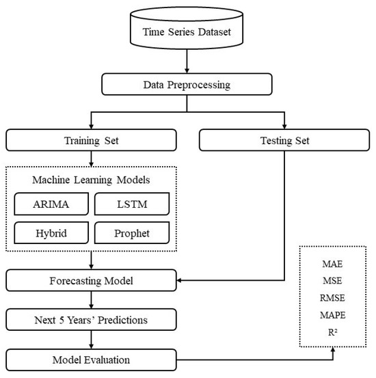
Figure 1.
Research process.
The dataset was divided into training (80%) and testing (20%) subsets to ensure robust model evaluation. This partitioning strategy ensures that the models are trained on historical cancer incidence data while reserving a separate portion for performance evaluation.
The models were trained using historical data (1992–2016) and validated with a test set (2017–2021). Once validated and finalized, each model (ARIMA, LSTM, Prophet, hybrid ARIMA-LSTM) was then used to forecast the number of new cancer cases and incidence rates sequentially for future years (2022 to 2026).
The study implemented a validation procedure for forecasting models, including time series cross-validation. Due to the sequential nature of data, traditional random cross-validation methods are not used, and 10-fold cross-validation must be used to verify the time series. This process is repeated by moving the cutoff point through the time series to ensure that each model’s performance is tested in different periods and conditions.
Evaluation metrics such as mean absolute error (MAE), mean squared error (MSE), root mean squared error (RMSE), and R-squared (R2) were calculated on the test set to assess prediction accuracy.
3.2. Data Source
This study obtained data on cancer incidence from the Canadian Cancer Registry Tabulation Master File, which Statistics Canada released on 31 January 2024. The table includes cancer cases diagnosed from 1992 to 2021 and is available by cancer type, region, age group, and sex.
The Canadian Cancer Registry (CCR) is a population-based registry with data collected and reported to Statistics Canada by each provincial/territorial cancer registry. This person-based system aims to collect information about each new primary cancer diagnosed among Canadian residents since 1992 [24]. Cancer incidence refers to the number of new cancers in a population during a specific period (usually a year). It is generally expressed as the number of new cancer cases per 100,000 population. Data presented in [25] were age-adjusted using the 2011 Canadian standard population to ensure accuracy and consistency [24].
3.3. Data Preprocessing
Prior to model training and evaluation, several preprocessing steps were applied to ensure data quality and model compatibility:
3.3.1. Handling Missing Data
Quebec’s cancer incidence data was unavailable after 2017 due to incomplete sub-missions to the Canadian Cancer Registry. To address this gap, Quebec’s missing incidence data from 2018 to 2022 were imputed using a multiple imputation strategy based on available historical trends and region-specific cancer patterns. Other provinces with minor missing values, less than 3% of the data, were handled using multiple imputations again.
3.3.2. Normalization
To ensure consistency across features and models, all incidence rate and case count values were normalized using min-max scaling to a range between 0 and 1. This was especially important for neural network models (e.g., LSTM), which are sensitive to the scale of input features. Normalization helped stabilize the training process and improve model convergence.
3.3.3. Temporal Indexing
Dates were converted into a standardized time index to ensure uniform time series input formats across all models, especially for ARIMA and Prophet, which require a consistent datetime structure.
3.3.4. Stationarity Checks
For models like ARIMA and ARIMA-LSTM, stationarity was assessed using the Augmented Dickey–Fuller test. Non-stationary series were differenced as required to satisfy model assumptions.
These preprocessing steps were essential for maintaining data integrity and enabling fair comparison across diverse model architectures.
3.4. Model Selection
To investigate the trends in cancer incidence in this study, four popular machine learning algorithms and statistical techniques for time series prediction were selected based on their proven track record in time series forecasting: Prophet, long short-term memory (LSTM) networks, autoregressive integrated moving average (ARIMA), and the hybrid ARIMA-LSTM model.
3.4.1. Long Short-Term Memory (LSTM)
Introduced by Hochreiter and Schmidhuber in 1997 [26], LSTM networks are a variant of RNNs that overcome the shortcomings of standard RNNs. These disadvantages include poor performance in handling long-term dependencies and the vanishing or exploding gradient problem. In 1999, a forgotten gate was added to LSTM to restore cell memory, improve the original structure, and become the standard structure for LSTM networks. Unlike deep feedforward neural networks (DFNN), LSTMs contain feedback connections and can process data sequences, not just individual data points such as vectors or arrays [27].
In LSTM networks, the fundamental building block is called a memory block or LSTM unit. Composed of a cell that acts as the memory component and three gates (input, output, forget/keep), these units can retain information over arbitrary periods. The gates of the LSTM unit are responsible for regulating the flow of data through the cell. One of the most prominent features of the LSTM cell is the “constant error carousel” (CEC). An LSTM network is structured similarly to an RNN, except the hidden layers comprise memory blocks instead of neurons [27].
Input gate: The unit features a sigmoidal function that regulates the inflow of data into the cell. It obtains activation from the previous output h(t−1) and the current input x(t). By means of the sigmoid function, an input gate produces values ranging from zero to one. A value of zero acts as a complete blockage of information, while a value of one permits the passage of all information. Equation (1) shows this process [27].
Cell input layer: The input to the cell is like the input gate. It takes in the previously hidden state h(t−1) and the current input x(t). However, a “tanh” activation function is used to squash the input values to a range between −1 and 1, which is indicated by the symbol lt in the Equation (2) [27].
Forget gate: A unit using a sigmoidal function decides what information from previous steps of the cell should be remembered or discarded. The forget gate takes input from h(t−1) and x(t) and assumes values between zero and one. The next step involves a Hadamard product with the old cell state ct−1 to update to a new cell state ct in the below equation. If the forget gate has a value of zero, it is closed and will completely forget the information of the old cell state ct−1. On the other hand, the value of one will make all information memorable. Thus, the forget gate has the authority to reset the cell state if the old data are deemed irrelevant. Equation (3) summarizes the forget gate mechanism [27].
Cell state: The cell state is responsible for storing a cell’s memory over an extended period. Each cell contains a self-connected linear unit known as a constant error carousel (CEC), which recurrently operates to prevent the vanishing or exploding gradient problem in an LSTM network. The CEC incorporates a forget gate that regulates and resets the gate as needed. At time t, the present cell state ct is modified by the previous cell state ct−1, controlled by the forget gate, and the current input and cell input product (it ∘ lt). Equation (4) summarizes the overall update of a cell state [27].
Output gate: A unit equipped with a sigmoidal function has the ability to regulate the passage of information from a cell. In contrast, an LSTM network utilizes the output gate values at a particular time (represented by ot) to govern the present cell state ct, which is then stimulated by a “tanh” function to produce the ultimate output vector h(t). Equations (5) and (6) show the mechanism of the output gate [27].
3.4.2. Facebook Prophet Forecasting Model
Facebook’s Prophet network is a strong tool that can accurately predict time-series data using daily observations of patterns at different scales. Forecast time-series data are derived from additional models, where nonlinear trends account for seasonal, weekly, and daily periods, including holiday results. This tool works best during periods with stable seasonal results and a few seasons of historical data. Prophet deals with missing data and trend changes and can often adapt to deviations. It allows users to make more accurate forecasts faster than other time series forecasting strategies, requiring very little computer time. Prophet is at the level of other models and quickly generates predictions in seconds. This tool can be used to generate accurate weather forecasts even from incomplete or black data without manual work. In addition, the Prophet has many “human” seasons of the week and year [28,29].
As a powerful tool for Python and R released in 2017 by Facebook, Prophet models time series datasets with trends, seasonality, and holidays. Prophet takes a few seconds to fit the model with tunable parameters, and it is represented by the Formula (7) [30]:
The equation provides a comprehensive prediction formula for the Prophet forecasting model, wherein the anticipated outcome, y(t), is determined by the linear or logistic equation, g(t); seasonality based on the chosen period, such as yearly, monthly, or daily, is denoted as s(t); holiday-related anomalies are denoted as h(t); and unforeseen errors are denoted as ϵt. The model encompasses multiple parameters that can be fine-tuned to enhance forecasting accuracy. Depending on the intended use, the model can be classified as linear or logistic. Linear models normalize outliers and do not impose a maximum or minimum threshold. Conversely, logistic models are suitable for saturated forecasts that require defining the highest and lowest values [30].
3.4.3. Autoregressive Integrated Moving Average (ARIMA)
ARIMA, a classic statistical model, uses patterns such as trends and seasonality to predict future scores in a series. It is a generalized version of the ARMA model specially designed to handle non-stationary time series. Unlike the ARMA model, which assumes stationarity of the analyzed time series, non-stationary time series must first undergo a transformation process to remove seasonality and trends through finite-point differentiation. A stationary time series is a combination of signal and noise. The ARIMA model separates the time signal from the noise and gives its forecast for a later time point. As indicated by the method’s acronym, its structural components are the following [31,32]:
AR for autoregression: a regression model that uses the dependence relationship between an observation and several lagged observations (model parameter p).
I for integration: calculating the differences between observations at different time points (model parameter d), aiming to make the time series stationary.
MA for moving average: this approach considers the dependence that may exist between observations and the error terms created when a moving average model is used on observations that have a time lag (model parameter q) [33].
One way to represent an AR model with order p, or AR (p), is through a linear process, as shown in Equation (8). The stationary variable is denoted by x and the constant by c. The autocorrelation coefficients at lags 1, 2, …, p are represented by ∅, while the residuals are the Gaussian white noise series with a mean of zero and a variance of σ [34].
Equation (9) represents an MA (q) order model, wherein the θ terms denote the weights given to the current and previous values of a stochastic term in the time series. Here, μ is the expectation of x and is generally assumed to be zero, while θ equals one. We consider ε to be a Gaussian white noise series with a mean of zero and variance of σ [34].
Equation (10) shows how these two models are combined to create an ARMA model of order (p, q), where ∅ ≠ 0, θ ≠ 0, and σ > 0. The parameters represent the AR and MA orders p and q, respectively. ARIMA forecasting, also known as Box and Jenkins forecasting, can handle non-stationary time series data due to its “integration” step. This step involves differencing the time series, converting a non-stationary time series into a stationary one [34].
3.4.4. ARIMA-LSTM Hybrid Model
The hybrid ARIMA-LSTM model is designed to capture the linear and nonlinear aspects of time series data. The time series must be stationary to apply the ARIMA model and predict future values. It should be checked with the Dickey–Fuller test to see if it is in place, and it should be performed if it is not already. Then, optimal parameters will be found to build the model, and finally, predictions will be made using the built model. LSTM works well for non-stationary parts of data as well as has relatively larger memory. The residuals obtained from ARIMA are fed into an LSTM model and trained to tap the pattern and predict the residuals for the next future period [35].
These two models have been chosen for their ability to break down a time series into linear and nonlinear trends, as expressed by Equation (11). In this equation, Lt illustrates the linear component of the time series at time step t. Also, Nt defines the nonlinear component, and ɛt represents the error term in the xt time series [36].
xt = Lt + Nt + ɛt
The reason for choosing different types of algorithms to conduct the research was to include the wide range of data found in cancer rate numbers and new case amounts and incidence rates with different qualities. LSTM networks provide flexibility in understanding long-term connected changes and complex patterns common in information. As a time-series analysis model, Prophet’s ability to deal with unexpected values, missing data, and shifting trends is beneficial for the unpredictable nature of healthcare information, like cancer-related datasets. As a statistical analysis model, ARIMA is strong at examining and predicting linear sequences and is vital for ensuring that a complete analytical method can compare against more complex models.
3.5. Evaluation Metrics
This study selected a suite of evaluation metrics that best represent the models’ forecasting accuracy, reliability, and applicability in a real-world context to comprehensively assess machine learning models, including LSTM, Prophet, and ARIMA, deployed in forecasting cancer incidence trends in Canada.
Different criteria, such as forecast error measurements, the speed of calculation, interpretability, and others, have been used to assess forecasting quality, where y is the measured value at time t. Forecast error measures or forecast accuracy are the most important in solving practical problems. Typically, the commonly used forecast error measurements are applied to estimate the quality of forecasting methods and choose the best forecasting mechanism for multiple objects. Despite their drawbacks, a set of “traditional” error measurements in every domain is applied. These error measurements are used as presets in domains despite the drawbacks. This section provides an analysis of existing and quite common forecast error measures that are used in forecasting. Measures are divided into groups according to the calculating method and value of error for a specific time t. The formula for calculating and the names of assessments are considered for each error measure [37].
3.5.1. Mean Absolute Error (MAE)
MAE measures the average magnitude of absolute errors between actual and predicted values. Lower MAE values indicate better accuracy. It is widely used in forecasting tasks because it provides an intuitive measure of prediction error in the same unit as the data.
Mean Absolute Error, is given by [37]:
where n is the number of observations, Fi is the forecasted value for observation i, and Ai is the actual value for observation i.
3.5.2. Mean Squared Error (MSE)
MSE calculates the average squared difference between actual and predicted values. MSE penalizes significant errors more heavily, making it useful for detecting significant deviations in predictions.
Mean Squared Error, is given by [37]:
where n is the number of observations, Fi is the forecasted value for observation i, and Ai is the actual value for observation i.
3.5.3. Root Mean Squared Error (RMSE)
RMSE is the square root of MSE, which provides an interpretable error value in the same unit as the target variable. RMSE is sensitive to large errors and is commonly used in forecasting applications to measure model performance.
Root Mean Squared Error is given by [37]:
where n is the number of observations, Fi is the forecasted value for observation i, and Ai is the actual value for observation i.
3.5.4. Mean Absolute Percentage Error (MAPE)
MAPE expresses the prediction error as a percentage of actual values, making it easier to interpret in relative terms. As it provides a percentage-based error measure, MAPE is particularly useful for comparing errors across datasets with different scales.
Mean Absolute Percentage Error is given by [37]:
where n is the number of observations, Fi is the forecasted value for observation i, and Ai is the actual value for observation i.
3.5.5. Coefficient of Determination (R2)
R2 represents the proportion of variance in the dependent variable that is predictable from the independent variables.
The Coefficient of Determination is given by:
R², or the coefficient of determination, is a widely used metric in regression analysis. It measures the proportion of the variance in the dependent variable that is predictable from the independent variables. However, it has limitations, such as being biased statistics and providing invalid results in the presence of measurement errors. Therefore, while R-squared is a valuable metric, it should be interpreted cautiously and in conjunction with other criteria [38]. It is widely used in regression and forecasting models to indicate how well the model explains the variability in the data. A value closer to 1 indicates a better fit.
R2 is not always suitable for time series forecasting due to the complex nature of time series data and the potential for model uncertainty. Goel [39] highlights the need for hybrid models that can capture both linear and nonlinear components in time series data, suggesting that a single metric like R2 may not adequately capture the predictive performance. Chatfield [40] further emphasizes the importance of considering model uncertainty in time series analysis, which can affect the accuracy of forecasts. Hewamalage [41] underscores the need for robust and efficient forecasting methods, indicating that R2 may not be the most suitable metric in all cases. Lastly, Kim [42] discusses the impact of estimation error on forecast mean squared errors, which can also affect the reliability of R2 in time series forecasting.
The limitations mentioned regarding the R2 metric, such as potential bias and sensitivity to measurement errors, are intended to highlight practical issues related to real-world model interpretation and data quality considerations. Specifically, R2 can be influenced by factors such as model specification, omitted variables, and data inaccuracies, rather than being inherently flawed mathematically. Therefore, R2 values should always be interpreted with careful attention to these practical and contextual limitations, especially in complex forecasting scenarios.
4. Results
4.1. Performance of the Models
After deploying all models for every category, evaluation metrics were extracted to assess the models’ performance. The results help us to choose the best models for categories. This section gives the error rates for each model for forecasting new cancer cases and incidence rates for 2022 to 2026 for different categories. The models were trained on data from 1992 to 2021.
It is important to note that negative R2 values, as observed for the Prophet model in our analysis, indicate that the model does not improve predictive accuracy compared with a baseline mean-only (intercept-only) model. Such results do not inherently suggest that the Prophet model is incorrectly specified or invalid. Rather, these negative values highlight that, within the specific context of our forecasting problem, the Prophet model’s predictive strength was comparatively weaker than the other evaluated models (ARIMA, LSTM, and Hybrid ARIMA-LSTM). Therefore, R2 values, particularly negative ones, should be interpreted cautiously as indicators of relative model performance rather than absolute measures of model validity.
4.1.1. Error Rates for Geography Categories
Table 1 shows the error rates for new cancer cases and cancer incidence rates in geographical regions. The error rates have been interpreted to indicate the best models, which have been highlighted in bold and italic. The error rates show that the hybrid model performs the best in forecasting new cancer cases and cancer incidence rates for geographic regions.

Table 1.
Error rates of geography regions for new cancer cases and cancer incidence rate.
4.1.2. Error Rates for Age Categories
Table 2 shows the error rates for new cancer cases and cancer incidence rates in age group categories. The error rates have been interpreted to indicate the best models, indicated by bold and italic highlights. The error rates show that the hybrid model performs the best in forecasting new cancer cases and cancer incidence rates for age group categories.
Table 2.
Error rates of age group categories for new cancer cases and cancer incidence rate.
4.1.3. Error Rates for Sex Categories
Table 3 shows the error rates for new cancer cases and cancer incidence rate in sex categories. The error rates have been interpreted to indicate the best models, which have been highlighted in bold. The error rates show that the LSTM model performs the best in forecasting new cancer cases for sex categories.
Table 3.
Error rates of sex-based categories for new cancer cases and cancer incidence rate.
4.2. Forecasting New Cancer Cases and Incidence Rate
Among the other models, the hybrid model is the optimum model for predicting the values for geography categories from 2022 to 2026. Table 4 shows the results extracted from the mentioned model.
Table 4.
Predicted number of new cancer cases and cancer incidence rates by regions in Canada.
Compared with the other models, the hybrid model is the optimum model for predicting the values for age group categories from 2022 to 2026. Table 5 demonstrates the results extracted from the model mentioned.
Table 5.
Predicted number of new cancer cases and cancer incidence rate by age groups in Canada.
Compared with the other models, the LSTM model is the best model for forecasting the values for sex-based categories from 2022 to 2026. Table 6 shows the results extracted from the model mentioned.
Table 6.
Predicted number of new cancer cases and cancer incidence rate by sex in Canada.
4.3. Visualization Insights
Figure 2, Figure 3 and Figure 4 visually show the results of forecasted new cancer cases from 2022 to 2026 for regions, age groups, and sex, respectively.
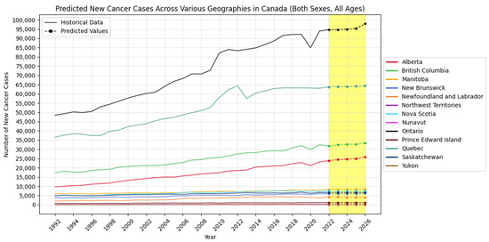
Figure 2.
Forecasted new cancer cases across various regions in Canada (the yellow-shaded area shows the predicted values).
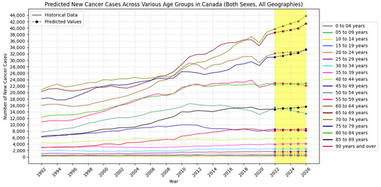
Figure 3.
Forecasted new cancer cases across various age groups in Canada (the yellow-shaded area shows the predicted values).
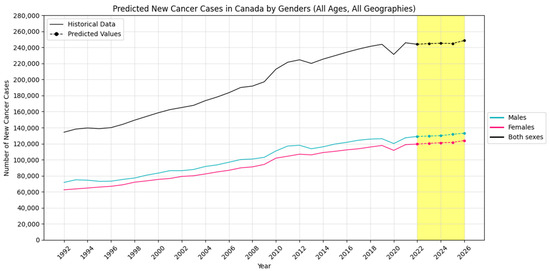
Figure 4.
Forecasted new cancer cases in Canada by sexes (the yellow-shaded area shows the predicted values).
Also, Figure 5, Figure 6 and Figure 7 visually show the results of the forecasted cancer incidence rate per 100,000 people from 2022 to 2026 for regions, age groups, and sexes, respectively.
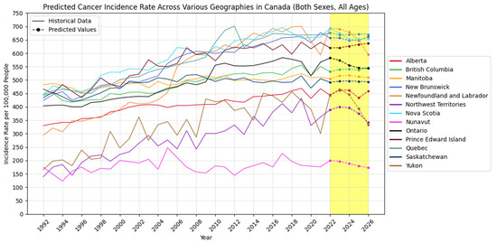
Figure 5.
Forecasted cancer incidence rate per 100,000 people across various regions in Canada (the yellow-shaded area shows the predicted values).
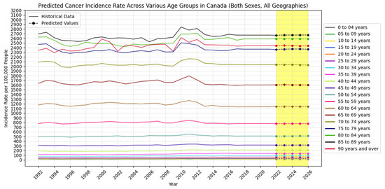
Figure 6.
Forecasted cancer incidence rate per 100,000 people across various age groups in Canada (the yellow-shaded area shows the predicted values).
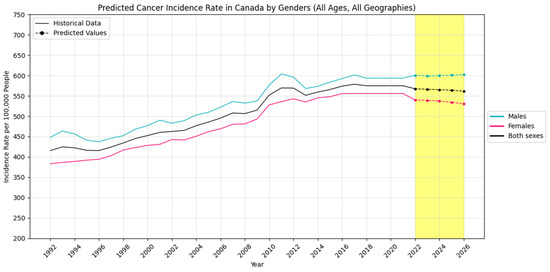
Figure 7.
Forecasted cancer incidence rate per 100,000 people in Canada by sex (the yellow-shaded area shows the predicted values).
5. Discussion
The findings of this study align with previous research on cancer incidence forecasting in Canada but extend existing methodologies by incorporating machine learning (ML) models to enhance predictive accuracy. Past studies, such as those by Brenner et al. [16,17,18], have relied heavily on statistical models like CANPROJ, which use age-period-cohort (APC) frameworks to extrapolate trends. While effective in capturing historical linear patterns, such models assume that past trends will continue predictably, limiting their ability to reflect complex, nonlinear dynamics in cancer data. In contrast, the machine learning models used in this study, particularly the hybrid ARIMA-LSTM model, are adaptive and data-driven, capable of learning from fluctuations and underlying patterns that may not follow a strict statistical progression.
For instance, Brenner et al. projected new cancer cases up to 2024 using historical data and demographic adjustments. Our approach not only extends these projections to 2026, offering a more updated outlook, but also improves accuracy by integrating deep learning with statistical time series models. The hybrid ARIMA-LSTM model consistently yielded lower error rates than other models, demonstrating that this combined approach effectively captures both linear and nonlinear trends in cancer incidence forecasting.
The analysis reveals distinct patterns and trends across sex, geography, and age groups. Males exhibit a steady increase in both new cancer cases and incidence rates, while females experience a rise in absolute cases but a decline in incidence rates.
The observed trend in female cancer incidence—where absolute cancer cases are increasing while incidence rates are declining—suggests demographic shifts, notably population growth and aging, rather than improvements in cancer treatments alone. Additionally, improvements in screening programs and early detection efforts (such as breast and cervical cancer screening) documented in the existing literature likely play a role in stabilizing or reducing incidence rates for certain cancer types.
Brenner et al. confirmed that despite an overall decline in cancer incidence and mortality rates, Canada is expected to see an increase in new cancer cases and deaths in 2024, primarily due to its growing and aging population. While advancements in prevention, screening, and treatment have mitigated the effects of certain cancers, these near-term projections emphasize the ongoing burden cancer may pose to individuals and the Canadian healthcare system [18].
Geographically, regions like Alberta, British Columbia, Ontario, and Quebec show increasing cancer cases and incidence rates, indicating a growing cancer burden. In contrast, provinces such as Newfoundland and Labrador demonstrate a declining trend, possibly reflecting effective local cancer control measures or public health strategies. Age-wise, cancer incidence remains stable among children but increases significantly among middle-aged and older adults, especially in individuals aged 75 and above.
These findings underscore the need for targeted public health interventions explicitly tailored to demographic groups and geographic regions showing an increased cancer burden. The steady rise in cancer cases among older adults and specific provinces highlights the importance of developing age-specific and region-specific cancer prevention and control strategies. Meanwhile, stability in pediatric cancer incidence suggests that existing pediatric cancer strategies may be effective but require sustained support.
Given the complexity of cancer incidence trends, selecting an accurate forecasting model is critical for public health planning. An evaluation of model performance reveals that the hybrid ARIMA-LSTM model consistently achieves the lowest error rates across most geographic and age group categories, making it the most suitable choice for cancer incidence forecasting. This model outperforms the ARIMA, LSTM, and Prophet models in key accuracy metrics, including MAE, MSE, RMSE, MAPE, and R².
5.1. Model Performance Across Demographics and Regions
Geographic performance: The hybrid ARIMA-LSTM model yields significantly lower RMSE values across multiple provinces, with R2 values exceeding 0.80 in most cases, indicating strong predictive accuracy. In contrast, the Prophet model exhibits the highest error rates, often producing negative R² values, suggesting poor model fit.
Age group performance: The hybrid model provides the most accurate predictions for middle-aged and older adults (50+ years), achieving the lowest MAPE and RMSE values. In contrast, the Prophet model underperforms in most age categories.
Gender performance: While the hybrid model excels in most categories, LSTM performs best in gender-based forecasting, particularly for male and female cancer incidence rates, as indicated by its superior MAE and RMSE values.
The hybrid ARIMA-LSTM model’s superior performance is attributed to its ability to capture both linear and nonlinear trends in cancer incidence data. ARIMA alone is well suited for handling linear trends but struggles with complex patterns, whereas LSTM excels in capturing long-term dependencies. By integrating these approaches, the hybrid model effectively mitigates their individual limitations, resulting in more accurate and reliable cancer incidence forecasts.
5.2. Implications for Public Health and Cancer Prevention
The findings highlight the critical role of advanced forecasting models in improving cancer prevention and resource allocation strategies. Rising incidence rates in middle-aged and older adults necessitate robust screening programs and preventive measures tailored to these demographics. Similarly, region-specific public health initiatives that address unique risk factors are essential to mitigating the cancer burden. By leveraging accurate forecasting models, policymakers and healthcare professionals can develop more effective intervention strategies, optimize resource allocation, and ultimately improve cancer outcomes across diverse populations.
Our study provides a foundation for further integrating AI-driven forecasting models in epidemiological research. Future research could explore ensemble methods, combining traditional epidemiological models (e.g., APC) with deep learning architectures to refine cancer incidence predictions further. Additionally, incorporating real-time clinical and genetic data could enhance prediction accuracy and improve personalized cancer risk assessments.
5.3. Limitations
One of the key limitations of this study is the imputation of Quebec’s cancer incidence data after 2017 due to the absence of official records. While we employed a multiple imputation approach to enhance accuracy and capture uncertainty, projections remain dependent on historical trends and national averages rather than direct registry data. The variability in imputed estimates reflects the inherent uncertainty in forecasting missing data. Future studies should integrate officially updated Quebec data when available to refine predictive models further and validate imputed estimates.
Also, this study analyzes cancer incidence as a whole, whereas prevention programs typically target specific cancers. Future research should extend this analysis to individual cancer types, allowing for a more detailed examination of how prevention efforts impact site-specific cancer trends.
Moreover, our study assumes that biological and environmental factors primarily drive cancer incidence trends, but access to healthcare services plays a crucial role in early detection and diagnosis. Screening disparities, specialist availability, and healthcare system delays may introduce biases in observed cancer incidence rates across age groups and regions. Future studies should incorporate healthcare accessibility indices to better quantify the role of healthcare infrastructure in shaping cancer trends.
Author Contributions
Conceptualization, E.K. and K.P.; methodology, E.K. and K.P.; software, E.K.; validation, E.K. and K.P.; formal analysis, E.K.; investigation, E.K.; resources, E.K. and K.P.; data curation, E.K.; writing—original draft preparation, E.K.; writing—review and editing, E.K. and K.P.; visualization, E.K.; supervision, K.P.; project administration, K.P.; funding acquisition, K.P. All authors have read and agreed to the published version of the manuscript.
Funding
This research received no external funding.
Data Availability Statement
The original data presented in the study are openly available in the Statistics Canada portal, published on 31 January 2024 at this link https://www150.statcan.gc.ca/n1/daily-quotidien/240131/dq240131d-eng.htm.
Conflicts of Interest
The authors declare no conflicts of interest.
References
- Kibbe, W.A.; Klemm, J.D.; Quackenbush, J. Cancer Informatics: New Tools for a Data-Driven Age in Cancer Research. Cancer Res. 2017, 77, e1–e2. [Google Scholar] [CrossRef] [PubMed][Green Version]
- Biemar, F.; Foti, M. Global progress against cancer—Challenges and opportunities. Cancer Biol. Med. 2013, 10, 183–186. [Google Scholar] [CrossRef] [PubMed]
- Sikora, K. Developing a global strategy for cancer. Eur. J. Cancer 1999, 35, 24–31. [Google Scholar] [CrossRef] [PubMed]
- Ivanović, M.; Radovanović, M. Modern machine learning techniques and their applications. In Electronics, Communications and Networks IV; CRC Press: Boca Raton, FL, USA, 2015. [Google Scholar] [CrossRef]
- Rathor, A.; Gyanchandani, M. A review at Machine Learning algorithms targeting big data challenges. In Proceedings of the 2017 International Conference on Electrical, Electronics, Communication, Computer, and Optimization Techniques (ICEECCOT), Mysuru, India, 15–16 December 2017; pp. 1–7. [Google Scholar] [CrossRef]
- Nguyen, G.T.; Dlugolinsky, S.; Bobák, M.; Tran, V.D.; López García, Á.; Heredia, I.; Malík, P.; Hluchý, L. Machine Learning and Deep Learning frameworks and libraries for large-scale data mining: A survey. Artif. Intell. Rev. 2019, 52, 77–124. [Google Scholar] [CrossRef]
- Udousoro, I.C. Machine Learning: A Review. Semicond. Sci. Inf. Devices 2020, 2, 5–14. [Google Scholar] [CrossRef]
- Verma, M.; Khoury, M.J.; Ioannidis, J.P. Opportunities and Challenges for Selected Emerging Technologies in Cancer Epidemiology: Mitochondrial, Epigenomic, Metabolomic, and Telomerase Profiling. Cancer Epidemiol. Biomark. Prev. 2012, 22, 189–200. [Google Scholar] [CrossRef]
- Berger, M.L.; Curtis, M.D.; Smith, G.; Harnett, J.; Abernethy, A.P. Opportunities and challenges in leveraging electronic health record data in oncology. Future Oncol. 2016, 12, 1261–1274. [Google Scholar] [CrossRef]
- Gupta, S.; Gupta, A.; Kumar, Y. Artificial intelligence techniques in Cancer research: Opportunities and challenges. In Proceedings of the 2021 International Conference on Technological Advancements and Innovations (ICTAI), Tashkent, Uzbekistan, 10–12 November 2021; pp. 411–416. [Google Scholar] [CrossRef]
- Schlick, C.J.; Castle, J.P.; Bentrem, D.J. Utilizing Big Data in Cancer Care. Surg. Oncol. Clin. N. Am. 2018, 27, 641–652. [Google Scholar] [CrossRef]
- Shweta; Riya; Kumar, A. Cancer Prediction Using Machine Learning Algorithm. Int. J. Sci. Res. (IJSR) 2022, 11, 873–875. [Google Scholar] [CrossRef]
- Kaur, I.; Doja, M.N.; Ahmad, T. Data mining and machine learning in cancer survival research: An overview and future recommendations. J. Biomed. Inform. 2022, 128, 104026. [Google Scholar] [CrossRef]
- Shruti Trivedi, N.K. Predictive Analytics in Healthcare using Machine Learning. In Proceedings of the 2023 14th International Conference on Computing Communication and Networking Technologies (ICCCNT), Delhi, India, 6–8 July 2023; pp. 1–5. [Google Scholar] [CrossRef]
- Meropol, N.J.; Donegan, J.; Rich, A.S. Progress in the Application of Machine Learning Algorithms to Cancer Research and Care. JAMA Netw. Open 2021, 4, e2116063. [Google Scholar] [CrossRef] [PubMed]
- Brenner, D.R.; Poirier, A.; Woods, R.R.; Ellison, L.F.; Billette, J.M.; Demers, A.A.; Zhang, S.X.; Yao, C.; Finley, C.; Fitzgerald, N.; et al. Canadian Cancer Statistics Advisory Committee. Projected estimates of cancer in Canada in 2022. CMAJ 2022, 194, E601–E607. [Google Scholar] [CrossRef] [PubMed] [PubMed Central]
- Brenner, D.R.; Weir, H.K.; Demers, A.A.; Ellison, L.F.; Louzado, C.; Shaw, A.; Turner, D.; Woods, R.R.; Smith, L.M. Projected estimates of cancer in Canada in 2020. Can. Med. Assoc. J. 2020, 192, E199–E205. [Google Scholar] [CrossRef] [PubMed]
- Brenner, D.R.; Gillis, J.; Demers, A.A.; Ellison, L.F.; Billette, J.-M.; Zhang, S.X.; Liu, J.L.; Woods, R.R.; Finley, C.; Fitzgerald, N.; et al. Projected estimates of cancer in Canada in 2024. Can. Med. Assoc. J. 2024, 196, E615–E623. [Google Scholar] [CrossRef]
- Table 13-10-0394-01: Leading Causes of Death, Total Population, by Age Group. Statistics Canada: Ottawa, ON, Canada, 2025; Available online: https://www150.statcan.gc.ca/t1/tbl1/en/tv.action?pid=1310039401 (accessed on 4 August 2018).
- Canadian Cancer Statistics Advisory Committee in Collaboration with the Canadian Cancer Society Statistics Canada and the Public Health Agency of Canada. Canadian Cancer Statistics; Canadian Cancer Society: Toronto, ON, Canada, 2021; Available online: www.cancer.ca/Canadian-Cancer-Statistics-2021-EN (accessed on 28 March 2022).
- Xie, L.; Semenciw, R.; Mery, L. Cancer incidence in Canada: Trends and projections (1983–2032). Health Promot. Chronic Dis. Prev. Can. 2015, 35 (Suppl. S1), 2–186. [Google Scholar] [CrossRef]
- de Oliveira, C.; Weir, S.; Rangrej, J.; Krahn, M.D.; Mittmann, N.; Hoch, J.S.; Chan, K.K.W.; Peacock, S. The economic burden of cancer care in Canada: A population-based cost study. CMAJ Open 2018, 6, E1–E10. [Google Scholar] [CrossRef]
- Qiu, Z.; Hatcher, J. Cancer Projection Analytical Network Working Team CANPROJ: The Rpackage of Cancer Projection Methods Based on Generalized Linear Models for Age Period/or Cohort Version, I; Alberta Health Services: Edmonton, AB, Canada, 2013. [Google Scholar]
- Government of Canada, S.C. Cancer Incidence in Canada, 2021. The Daily. Available online: https://www150.statcan.gc.ca/n1/daily-quotidien/240131/dq240131d-eng.htm (accessed on 31 January 2024).
- Government of Canada, S.C. Canadian Cancer Registry—Age-Standardization: Incidence; Government of Canada, Statistics Canada: Ottawa, ON, Canada, 2025; Available online: https://www.statcan.gc.ca/en/statistical-programs/document/3207_D12_V4 (accessed on 17 November 2021).
- Hochreiter, S.; Schmidhuber, J. Long short-term memory. Neural Comput. 1997, 9, 1735–1780. [Google Scholar] [CrossRef]
- Emmert-Streib, F.; Yang, Z.; Feng, H.; Tripathi, S.; Dehmer, M. An Introductory Review of Deep Learning for Prediction Models with Big Data. Front. Artif. Intell. 2020, 3, 4. [Google Scholar] [CrossRef]
- Kaninde, S.; Mahajan, M.; Janghale, A.; Joshi, B. Stock Price Prediction using Facebook Prophet. ITM Web Conf. 2022, 44, 3060. [Google Scholar] [CrossRef]
- Korstanje, J. The Prophet Model. In Advanced Forecasting with Python; Apress: New York, NY, USA, 2021. [Google Scholar] [CrossRef]
- Shen, J.; Valagolam, D.; McCalla, S. Prophet forecasting model: A machine learning approach to predict the concentration of air pollutants (PM2.5, PM10, O3, NO2, SO2, CO) in Seoul, South Korea. PeerJ 2020, 8, e9961. [Google Scholar] [CrossRef]
- Rundo, F.; Trenta, F.; di Stallo, A.L.; Battiato, S. Machine learning for quantitative finance applications: A survey. Appl. Sci. 2019, 9, 5574. [Google Scholar] [CrossRef]
- Siami-Namini, S.; Tavakoli, N.; Namin, A.S. A comparison of ARIMA and LSTM in forecasting time series. In Proceedings of the 2018 17th IEEE International Conference on Machine Learning and Applications (ICMLA), Orlando, FL, USA, 17–20 December 2018; pp. 1394–1401. [Google Scholar]
- Kontopoulou, V.I.; Panagopoulos, A.D.; Kakkos, I.; Matsopoulos, G.K. A Review of ARIMA vs. Machine Learning Approaches for Time Series Forecasting in Data Driven Networks. Future Internet 2023, 15, 255. [Google Scholar] [CrossRef]
- Sima, S.N.; Akbar, S.N. Forecasting Economics and Financial Time Series: ARIMA vs. LSTM. arXiv 2018, arXiv:1803.06386. [Google Scholar] [CrossRef]
- Kulshreshtha, S.; Vijayalakshmi, A. An ARIMA-LSTM hybrid model for stock market prediction using live data. J. Eng. Sci. Technol. Rev. 2020, 13, 117–123. [Google Scholar] [CrossRef]
- Zhang, G.P. Time series forecasting using a hybrid ARIMA and neural network model. Neurocomputing 2003, 50, 159–175. [Google Scholar] [CrossRef]
- Maxim, S.; Adriaan, B.; Shcherbakova, N.L.; Anton, T.; Janovsky, T.A.; Kamaev, V.A. A survey of forecast error measures. World Appl. Sci. J. 2013, 24, 171–176. [Google Scholar]
- Cheng, C.; Shalabh Garg, G. Coefficient of determination for multiple measurement error models. J. Multivar. Anal. 2014, 126, 137–152. [Google Scholar] [CrossRef]
- Goel, H.; Melnyk, I.; Banerjee, A. R2N2: Residual Recurrent Neural Networks for Multivariate Time Series Forecasting. arXiv 2017, arXiv:1709.03159. [Google Scholar]
- Chatfield, C. Model uncertainty and forecast accuracy. J. Forecast. 1996, 15, 495–508. [Google Scholar] [CrossRef]
- Hewamalage, H.; Bergmeir, C.; Bandara, K. Recurrent Neural Networks for Time Series Forecasting: Current Status and Future Directions. arXiv 2019, arXiv:1909.00590. [Google Scholar] [CrossRef]
- Kim, T.; Leybourne, S.J.; Newbold, P. Asymptotic mean-squared forecast error when an autoregression with linear trend is fitted to data generated by an I(0) or I(1) process. J. Time Ser. Anal. 2004, 25, 583–602. [Google Scholar] [CrossRef]
Disclaimer/Publisher’s Note: The statements, opinions and data contained in all publications are solely those of the individual author(s) and contributor(s) and not of MDPI and/or the editor(s). MDPI and/or the editor(s) disclaim responsibility for any injury to people or property resulting from any ideas, methods, instructions or products referred to in the content. |
© 2025 by the authors. Licensee MDPI, Basel, Switzerland. This article is an open access article distributed under the terms and conditions of the Creative Commons Attribution (CC BY) license (https://creativecommons.org/licenses/by/4.0/).