Simulating Intraday Electricity Consumption with ForGAN

Abstract

Sparse data and an unknown conditional distribution of future values are challenges for managing risks inherent in the evolution of time series. This contribution addresses both aspects through the application of ForGAN, a special form of a generative adversarial network (GAN), to German electricity consumption data. Electricity consumption time series have been selected due to their typical combination of (non-linear) seasonal behavior on different time scales and of local random effects. The primary objective is to demonstrate that ForGAN is able to capture such complicated seasonal figures and to generate data with the correct underlying conditional distribution without data preparation, such as de-seasonalization. In particular, ForGAN does so without assuming an underlying model for the evolution of the time series and is purely data-based. The training and validation procedures are described in great detail. Specifically, a long iteration process of the interplay between the generator and discriminator is required to obtain convergence of the parameters that determine the conditional distribution from which additional artificial data can be generated. Additionally, extensive quality assessments of the generated data are conducted by looking at histograms, auto-correlation structures, and further features comparing the real and the generated data. As a result, the generated data match the conditional distribution of the next consumption value of the training data well. Thus, the trained generator of ForGAN can be used to simulate additional time series of German electricity consumption. This can be seen as a kind of proof for the applicabilty of ForGAN. Through a detailed descriptions of the necessary steps of training and validation procedures, a detailed quality check before the actual use of the simulated data, and by providing the intuition and mathematical background behind ForGAN, this contribution aims to demystify the application of GANs to motivate both theorists and researchers in applied sciences to use them for data generation in similar applications. The proposed framework has laid out a plan for doing so.

1. Introduction

A time series can be regarded as a sequence of correlated experiments where the result of the current experiment has an influence on the distribution of the following experiment’s result. Therefore, observing a time series needs time. Thus, data coming from a time series with a realistic length are typically sparse. This also makes the two classical tasks in the application of time series modeling, prediction of future values (forecasting) and simulation of different future realizations (generation of additional data), challenging.

The traditional literature on time series models such as autoregressive, ARIMA-type or regression-based models is mostly focused on prediction (see, e.g., [1,2] for the traditional time series approach). For this, an explicit functional relation between past values and the next value of the time series is assumed. Uncertainty typically enters via an additive error with zero expectation. Having estimated the parameters that determine the above-mentioned functional relation, the prediction of future values (given the past data) is uniquely determined. These methods often rely on assumptions such as linearity and stationarity, and they typically model uncertainty as Gaussian noise. As a result, they are poorly suited for capturing non-linear dependencies or generating diverse future scenarios, particularly when data are sparse or exhibit seasonal patterns.

Predicting the next value is also the typical task, even in state-of-the-art time series applications related to electricity consumption, production or $C{O}_2$ emissions (see, e.g., [3] for regression-based forecasts or [4] for a combination of periodic function approaches).

In contrast to these classical approaches, the focus here is not on the best prediction but on the approximation of the next element’s conditional distribution. This approach allows us to simulate a whole set of possible next elements for the same past data. No model is assumed for the time series evolution; instead, a purely data-based algorithm is provided.

However, when the full conditional distribution of the next value in a time series is needed, the traditional methods fail. They either typically generate the same value (given the past observations) or use an artificial model-based distribution, with the generated output deviating significantly from the true conditional distribution of the next value in the time series. However, when strategical decisions have to be taken, such as an enlargement or a partial reduction in the production capacity, it is important that not only the most likely next values are known but that the full underlying conditional distribution is also found.

At this point, so-called generative networks become relevant. Recent advancements in generative models, particularly generative adversarial networks (GANs), offer a promising approach for generating realistic synthetic data samples that closely follow the distribution underlying true data. This allows for an augmentation of a given dataset, helping the model to better capture complex patterns and improve the realism of simulated outcomes. GANs have achieved notable results in generating realistic samples in a variety of problem areas, such as producing real-looking images of human faces [5], translating one image to another (for example, photos of summer to winter [6] or day to night [7]), and 3D image generation [8]. Other research areas encompass speech synthesis [9] and video generation [10].

Although many of the above applications of GANs focus on static data, the focus here is on generating time series data. This shift in focus from static to sequential data requires architectures that can learn temporal data dependencies effectively. To describe the desired task and to demonstrate the application of our new method, the example of generating the next sequence of total electricity consumption per 15 min in Germany is considered.

This contribution focuses on ForGAN (see [11]), a conditional GAN (cGAN) specifically designed for time series simulations. The goal of ForGAN is to simulate the next value in a time series $x_{t+1}$, given the historical data $c=(x_1,\dots ,x_t)$. Unlike traditional forecasting models, ForGAN learns the underlying conditional probability distribution $p\left(x_{t+1}\right|c)$, enabling the generation of multiple plausible outcomes.

Again, this distinction between simulation and forecasting is crucial: forecasting aims to provide one single “best guess” for the future. Simulation explores the range of possible outcomes via simulating multiple realizations of $x_{t+1}$. Hence, ForGAN enables the generation of synthetic data for computing statistics or risk measures of $x_{t+1}$. Additionally, the set of generated values for $x_{t+1}$ can be used to compute a prediction for the actual value, such as the mode or the mean of the generated conditional distribution.

Given this task, the main innovations in this contribution are as follows:

• The accessible introduction of ForGAN as a well-suited data generation tool for time series data in applications related to electricity consumption.
• The presentation of our realization of ForGAN in detail and a display of its ability to learn the conditional distribution of a time series’ next value.
• To provide a framework that does not need data transformations nor parametric, simplistic model assumptions.
• The description of the full training process of ForGAN and its problems/dangers that have to be overcome.
• A collection of quality checks that a GAN has to pass before it is ready to generate reliable time series data.

The next section describes the basic structure and algorithms of a GAN in general. The focus will then shift to aspects of ForGAN. Accessible descriptions of its special structure and ingredients will be provided. In Section 3, ForGAN is presented in action by dealing with the problem of simulating the intraday electricity consumption data of Germany. These data are publicly available and are not as unpredictable as stock prices. They display a behavior in time that is a mixture of a (non-linear) deterministic tendency with moderate random fluctuations. A purely data-based approach is followed. In particular, it is not claimed that a new model for the behavior of energy consumption evolution has been found. The preprocessing of data before handing them to ForGAN is also explained. Further, hyperparameter tuning and algorithmic decisions before its application are considered. Section 4 demonstrates the effectiveness of ForGAN when applied to the time series of intraday electricity consumption data. By leveraging its ability to model true data distributions, ForGAN produces highly realistic simulations. This will be checked by testing it on the final $40\%$ of the time series.

The following sections aim to provide a comprehensive and reproducible example of how conditional GANs can be effectively adapted for time series simulations in real-world settings, such as electricity consumption forecasting. Finally, the results and properties of the method are discussed, and a conclusion is provided.

2. GANs and ForGAN: Idea, Structure and Algorithms

This section contains the introduction to the concept of GANs and explains their structure and the underlying algorithm, both on an intuitive and a mathematically sound level.

2.1. What Is a GAN?—A Heuristic Example

Generative adversarial networks (GANs), first proposed by Goodfellow et al. in 2014 [12], are an exciting architecture of deep neural networks. As already said in the introduction, GANs have been successfully applied for generating artificial data in various fields (see the references provided in the introduction). Therefore, GANs are often the first suggestion when one is lacking additional data to perform high-level statistics. However, it becomes evident that understanding their structure requires effort, and extensive training and testing are necessary before using them.

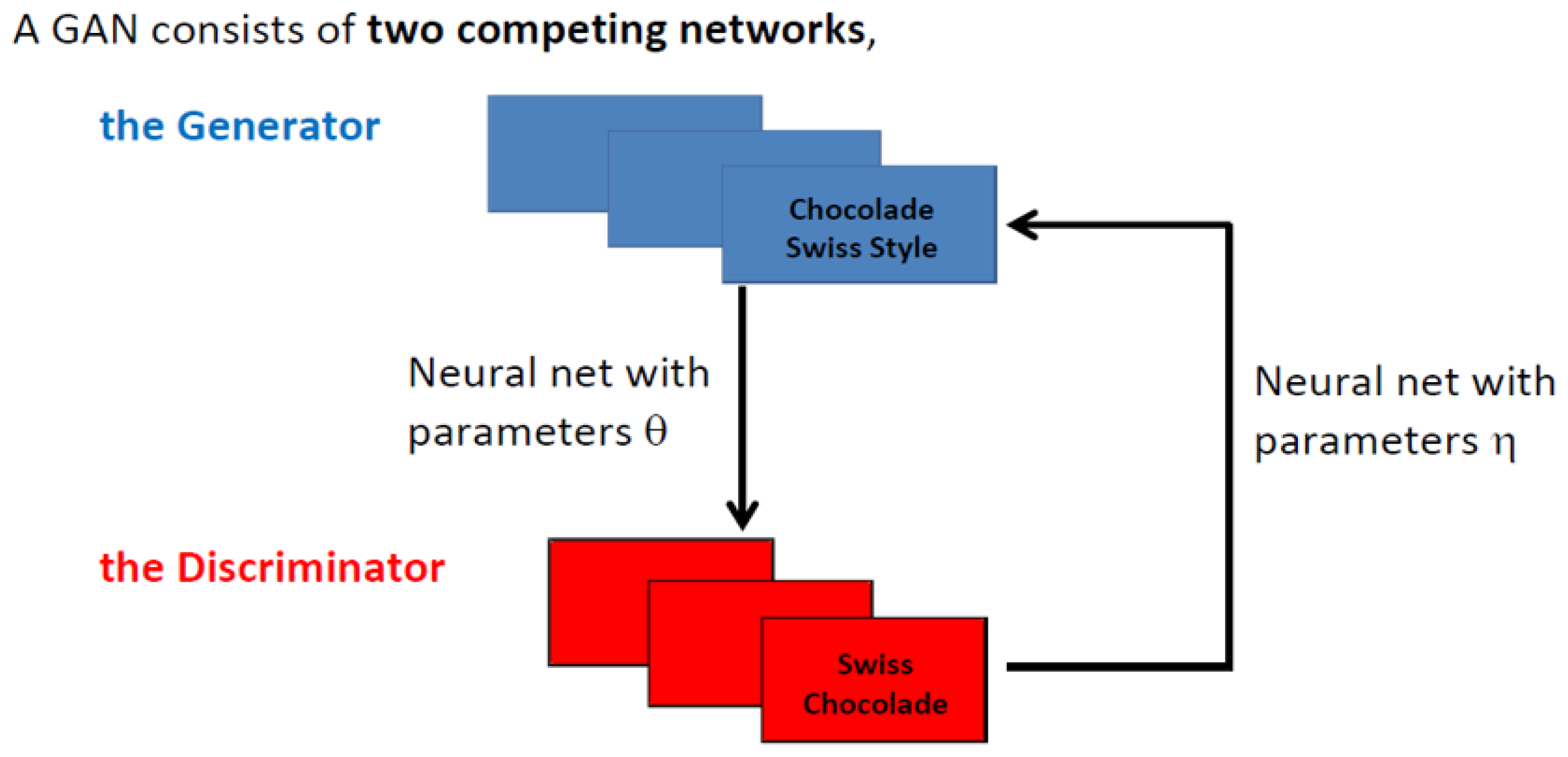
A helpful analogy for understanding GANs, presented in [13], involves a Swiss chocolate expert (the discriminator) who has tasted the finest Swiss chocolates but does not know the exact recipe. A foreign chocolate company (the generator) wants to replicate Swiss chocolate. The company produces batches of their chocolate and presents them to the expert for an evaluation together with batches from Swiss chocolate, as shown in Figure 1.

Each batch is tasted, and the expert provides feedback, such as the following:

• “This batch has too much sugar.”
• “This one has too much milk.”
• “The flavor needs less bitterness, but it could be Swiss chocolate.”

The expert’s role is to discriminate between real Swiss chocolate and the company’s attempt, offering constructive feedback and improving the discrimination ability, as feedback on the global quality of the judgment is provided afterward. The company adjusts its recipe and refines the chocolate with each iteration. Through repeated cycles, the company improves, producing chocolate so close to the original that it becomes nearly indistinguishable. Successful cooperation between the two players is essential for this process to work.

2.2. What Is a GAN?—The Mathematical Framework

As can be indicated from the heuristic example, a GAN has two ingredients or players. The first one (the generator) seeks to learn a probability distribution from a data sample. The generator will then be able to create (multivariate) random numbers with this distribution from (multivariate) standard Gaussian-distributed random numbers. For this task, a differentiable function $G\left(z\right):=G(z;{\theta }_G)$, which is represented by a deep neural network (multiple layer perceptron) with a parameter set ${\theta }_G$, will be fitted to the empirical distribution of the data sample.

The second one (the discriminator) seeks to find a discrimination strategy between data coming from an unknown distribution, the training data, and data that are generated by the generator. Data points will be classified as real or as fake, depending which of the two alternatives will be assigned a higher probability by the discriminator. The discriminator is given by a neural network $D\left(x\right):=D(x,{\theta }_D)$ with a parameter set ${\theta }_D$. $D\left(x\right)$ should output the probability that x is from the original dataset, which we denote by $x\sim p_{data}$. It can be seen as a generalization of a linear discriminant analysis.

While D will be trained to maximize the log-transformed probability $logD\left(x\right)$ that x is from the data of the training set, G is trained to minimize the (log-transformed) rejection probability $log(1-D(G\left(z\right)\left)\right)$ for z being from the noise distribution, which is denoted by $z\sim p_z$, where $p_z$ is a (multi-dimensional) Gaussian distribution with zero mean and unit variance.

The joint effort by the generator and the discriminator is modeled through a two-player min–max game between them of the following form (see [14]):

$$\underset{{\theta }_G}{min}\underset{{\theta }_D}{max}V(G,D)=\underset{{\theta }_G}{min}\underset{{\theta }_D}{max}{\mathbb{E}}_{x\sim p_{data}}[logD\left(x\right)]+{\mathbb{E}}_{z\sim p_z}[log(1-D\left(G\left(z\right)\right))],$$

(1)

where $V(D,G)$ is a binary cross-entropy function, commonly used in binary classification problems [15]. It is worth noting that the loss function in the min–max problem (1) has the aim to match the generator’s distribution $p_g$ (which is the result of transforming $p_z$ with $G(.)$) with the distribution of the real data $p_{data}$. The dependence of D and G from ${\theta }_G,{\theta }_D$ on the right side of the min–max problem is omitted for the simplicity of notation.

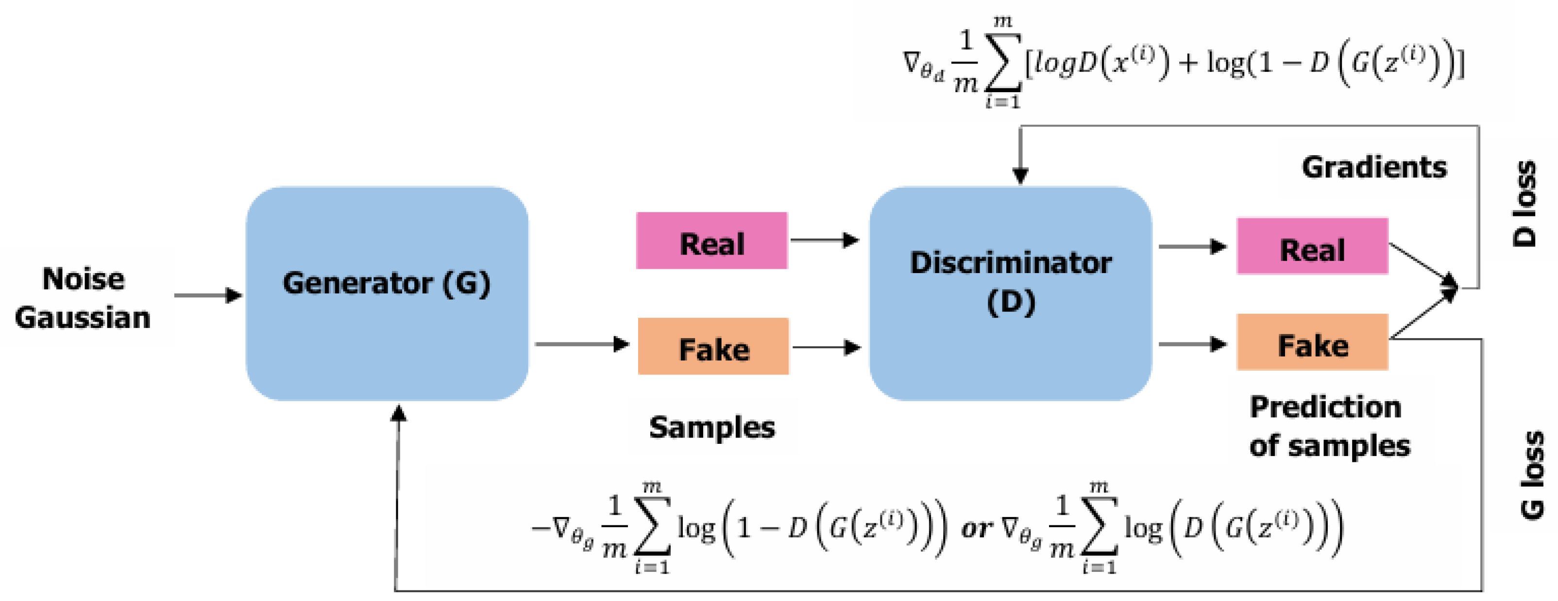
Of course, the expectations in (1) have to be estimated by the corresponding empirical means. The estimation is always based on subsamples (mini batches) of real and generated data of the same size m. Figure 2 below illustrates the basic architecture of a GAN. Here, the attribute generated is replaced by fake, as is often done in the literature. A further comment on the relation between the different objective functions of the discriminator and the generator is provided in Section 2.3 below. For more details on the mathematical background of GANs, we refer to [16].

2.3. Optimization Algorithm for Solving the Min–Max Problem

Before detailing the optimization approach, two special characteristics of GANs that differ from conventional networks should be noted (see also [17]). First, the cost function of a traditional neural network is explicitly determined in terms of its own trainable parameters $\theta$. However, in a GAN, the cost functions of both networks depend on two groups of trainable parameters, i.e., ${\theta }_D$ and ${\theta }_G$. Further, in a traditional neural network, one can tune all parameters during the training process. On the other hand, in GANs, each network can tune only its own weights and biases. This also needs a special sequential ordering of the training process.

Given the explicit form of the min–max problem (1), one can also define the separate objective functions of the discriminator and the generator as

$$\begin{array}{ccc}\hfill J_D({\theta }_D;{\theta }_G)& =& {\mathbb{E}}_{x\sim P_{\mathrm{data}}}[logD\left(x\right)]+{\mathbb{E}}_{z\sim p_z}[log(1-D\left(G\left(z\right)\right))]\hfill \end{array}$$

(2)

$$\begin{array}{ccc}\hfill J_G\left({\theta }_G\right)& =& {\mathbb{E}}_{z\sim p_z}[log(1-D\left(G\left(z\right)\right))]\hspace{1em}\hspace{1em}\hspace{1em}\hspace{1em}\hspace{1em}\hspace{1em}\hspace{1em}\hspace{1em}\hfill \end{array}$$

(3)

For solving the optimization problems in the min–max problem (1), a simultaneous gradient descent method is used. To update the parameters ${\theta }_D$, ${\theta }_G$, G and D are trained by backpropagating the loss through their respective models, which delivers the desired gradients. The following updating rules are obtained at step $t+1$ with $t\in \mathbb{N}$ for the parameter, respecting the order as

$${\theta }_D^{(t+1)}={\theta }_D^{\left(t\right)}+{\lambda }_t^D{▽}_{{\theta }_D}V(D^{\left(t\right)},G^{\left(t\right)})\mathrm{and}{\theta }_G^{(t+1)}={\theta }_G^{\left(t\right)}-{\lambda }_t^G{▽}_{{\theta }_G}V(D^{(t+1)},G^{\left(t\right)}),$$

(4)

where ${\lambda }_t^D,{\lambda }_t^D$ are the learning rates for discriminator and generator updates at step t, respectively. Note the minus sign in the update relation for ${\theta }_G$. This occurs as we minimize $J_G\left({\theta }_G\right)$. The choices of the learning rates are a highly researched subject in the calibration of neural networks in general. A detailed discussion is omitted here; however, the reader is referred to [18] for a detailed examination and recommendations of the choice of learning rates in GANs.

Remark 1.

Modifications of the gradient update

Goodfellow et al. (see [12]) suggest to use $k\in \mathbb{N}$ updating steps for ${\theta }_D$, followed by one updating step for ${\theta }_G$ to avoid overfitting of the discriminator. A further recommendation in [12] is to replace the objective function of the generator by

$$J_G\left({\theta }_G\right)={\mathbb{E}}_{z\sim p_z}[log\left(D\left(G\left(z\right)\right)\right)]$$

(5)

and maximizing it to avoid the gradient of the objective function to vanish too fast. This is used in the implementation presented here, which then results in the minus in the second relation of (4) to be replaced by a plus sign.

2.4. Time Series Generation with GANs

So far, the generator and discriminator adapt their strategies iteratively to learn an unknown underlying distribution. This, however, is in line with a sequence of i.i.d. data as the observed/training data. This is mainly the case in the applications that we referred to in the introduction.

Another field in which the application of GANs has been explored is finance. There, the data are typically given as time series data. In particular, the elements of the time series can be neither independent nor identically distributed. Thus, the data have to be prepared for the use of a GAN, i.e., one can deseasonalize or detrend the data. Moreover, one can perform (iterated) differencing before handing it over to the GAN and hope that the obtained data form an i.i.d. sequence.

An alternative to these conventional preprocessing methods is to learn a sequential dependence structure between data via a recurrent neural network. For instance, QuantGAN [19] introduces the use of a temporal convolutional network (TCN) to approximate volatility and capture long-range dependencies between variables for generating stock index time series data. More precisely, the TCN is utilized to learn the dependence of the next stock index return from a history of preceding returns—the conditioning window.

Apart from such a tailor-made construction, there also exist popular neural network structures such as LSTMs (long short-term memory networks; see [20]) or GRUs (gated recurrent networks; see [21]) networks, which are often used as standard tools for learning dependence structures. These architectures will also be used in the ForGAN framework.

2.5. ForGAN Architecture

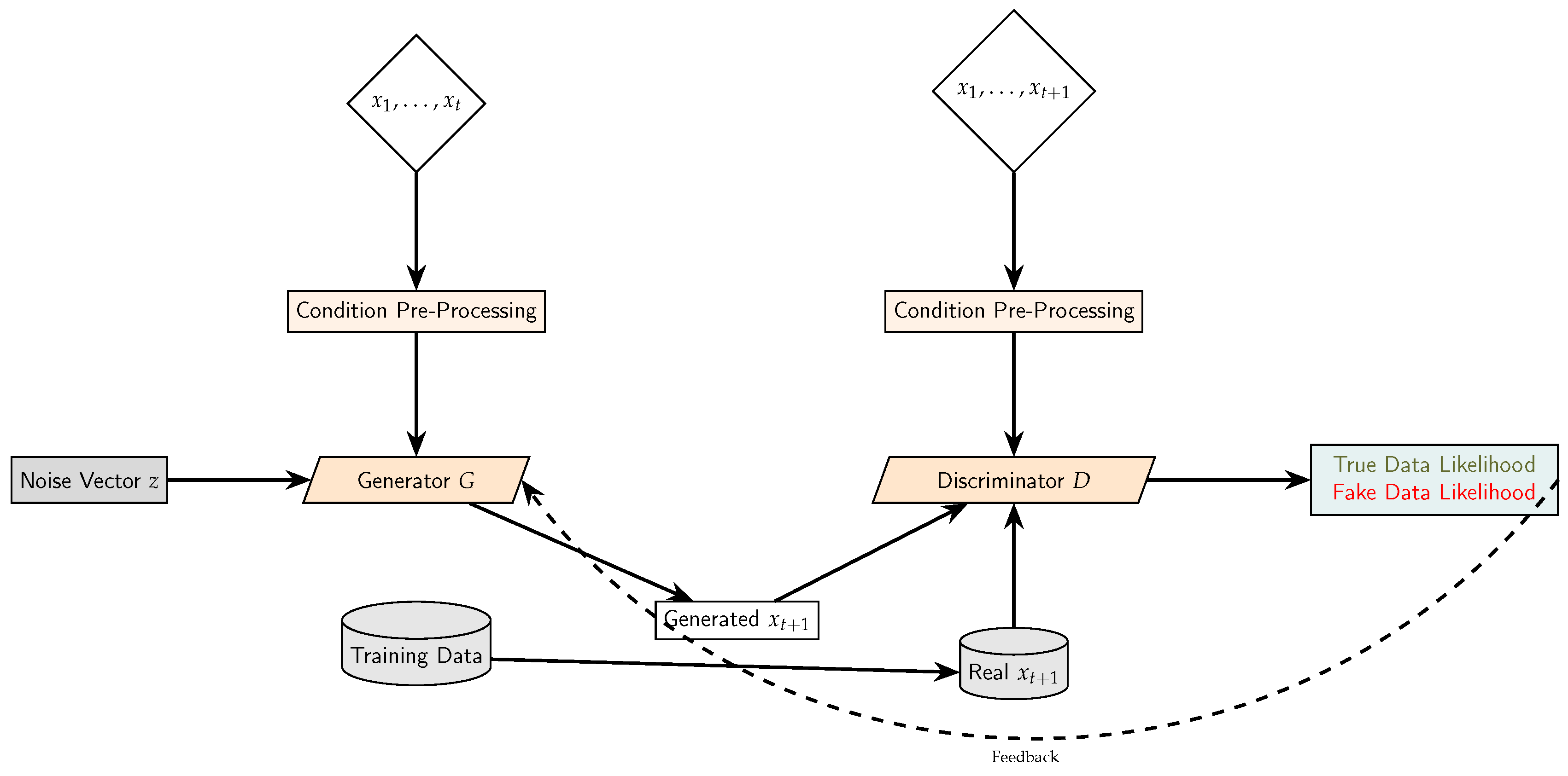
The primary difference between ForGAN and the standard GAN architecture is the conditional history c, which is provided to both the generator and discriminator. This condition contains information about the historical time series up to time t, enhancing the simulation of possible values for $x_{t+1}$. An illustration of the architecture of ForGAN is presented in Figure 3, and the different components shown in the figure are explained in the following subsections.

2.5.1. The Generator

The generator’s objective is to generate a forecast $x_{t+1}$ based on the condition $c=(x_1,\dots ,x_t)$, the historical time series data. To achieve this, the generator incorporates two main components:

• Condition-to-Latent Layer (LSTM or GRU)—Data preprocessing: This component makes the time series data ready for the use of a GAN. Assume a time series $x_1,x_2,\dots ,x_T$ is given. A GRU network is selected for learning the dependence structure of the time series. For a chosen fixed length k, all time windows $c=(x_{1+j},\dots x_{k+j})$ are considered with the goal of learning a lower-dimensional representation (the latent representation) $g(x_{1+j},\dots ,x_{k+j})\in {\mathbb{R}}^d$, where the size of d is also a chosen positive integer. This results in a training set of size $T-k-1$ for GRU to come up with a functional relationship between the condition window and its representation. In this implementation, a condition size of $k=96$, i.e., one full day of data and $d=32$, is used.
  Alternatively, the LSTM could have been selected for this data preparation step. Both the LSTM and GRU layers are effective at modeling sequential data by maintaining hidden states that capture long-range dependencies in time series. Also, there exist publicly available implementations of both the LSTM and GRU (see, e.g., Chapter 10 of [22]).
• Model (Sequential Neural Network): Given the latent representation of the input sequence, the generator combines this with random noise and passes the information through a series of fully connected layers to predict the next value in the series. More precisely, for each condition window $x_{1+j},\dots x_{k+j}$, the corresponding GRU-representation $g(x_{1+j},\dots x_{k+j})$ is taken and a standard normally distributed random variable $z_{k+1+j}$ of dimension N (with $N=32$ in this implementation) to come up with a generated next time series point $y_{k+1+j}$ via

  $$y_{k+1+j}=H_{{\theta }_G}\left(g(x_{1+j},\dots ,x_{k+j}),z_{k+1+j}\right).$$

  (6)
  Here, the function $H_{{\theta }_G}$ is a neural network with an input parameter of size $N+d=64$, which is a dense hidden layer of the same size that is then fully connected to the output layer of size 1. A ReLU function is used as an activation function. The network parameters ${\theta }_G$ of the generator network are then calibrated with the discriminator as normal in a standard GAN.
• Generation of a future path of the time series: Once the GAN is successfully trained, it can be used to generate a future path of the time series via

  $$y_S=H_{{\theta }_G}\left(g(x_{S-k-1},\dots ,x_{S-1}),z_S\right)$$

  (7)

  for some sequence of future values $y_S$, $S=T+1,T+2,\dots$ Here, the data history $x_{S-k-1},\dots ,x_{S-1}$ consists of elements from the real dataset as long as the indices are lower than or equal to T, while all data with an index higher than T are produced by the generator.

2.5.2. The Discriminator

The discriminator’s task is to distinguish between real and generated data. This is carried out by evaluating whether the generated data $y_{k+1+j}$ logically follow on from the historical data $c=(x_{1+j},\dots ,x_{k+j})$ or not. The discriminator incorporates two main components:

• Input-to-Latent Layer (LSTM or GRU): Like the generator, the discriminator uses an LSTM or GRU layer to process the combined sequence of historical data c and the next data point, either the real $x_{k+1+j}$ or the generated $y_{k+1+j}$. The ForGAN implementation involves a GRU different from the one used in the generator. As before, $k=96$ is used, resulting in a 97-dimensional input for the GRU. In this case, a latent representation $d(x_{1+j},\dots ,x_{97+j})\in {\mathbb{R}}^8$ of the relation between the conditioning window and the next value of the sequence.
• Model (Sequential Neural Network): The discriminator evaluates the authenticity of the input sequence by transforming the latent representation into a probability score, indicating whether the sample is real ($x_{k+1+j}$) or generated ($y_{k+1+j}$). A sigmoid activation function is used to compress this score between 0 and 1. More precisely, the discriminator has a simple neural network $D_{{\theta }_D}$ that applies a sigmoid activation function to an affine linear combination of the components of $d(x_{1+j},\dots ,u_{97+j})$ to obtain a probability for the last real component, i.e., $u_{97+j}=x_{97+j}$, and not a generated one. Again, the parameters ${\theta }_D$ are found during the training of the GAN.

2.6. Mathematical Formulation

The training of the ForGAN model follows a typical GAN framework. The generator and discriminator are trained in a min–max game, where the generator tries to minimize the loss by generating realistic predictions, while the discriminator attempts to maximize the loss by correctly distinguishing between real and fake data. The value function for this adversarial game is given by

$$\begin{array}{ccc}& & \underset{G}{min}\underset{D}{max}V(G,D)\hfill \\ & & =\underset{G}{min}\underset{D}{max}{\mathbb{E}}_{x_{t+1}\sim p_{data}\left(x_{t+1}\right)}[logD\left(x_{t+1}\right|c)]+{\mathbb{E}}_{z\sim p_z\left(z\right)}[log(1-D\left(G\left(z\right|c)\right))].\hfill \end{array}$$

Here, G denotes the generator network, D denotes the discriminator network, and $c=(x_1,\dots ,x_t)$ is the condition based on the historical data. Again, the dependence of G and D from their parameter vectors (${\theta }_G$, ${\theta }_D$) is omitted for ease of notation.

3. Experimental Setup: Data Description and Algorithmic Decisions

3.1. Dataset: Intraday Electricity Consumption

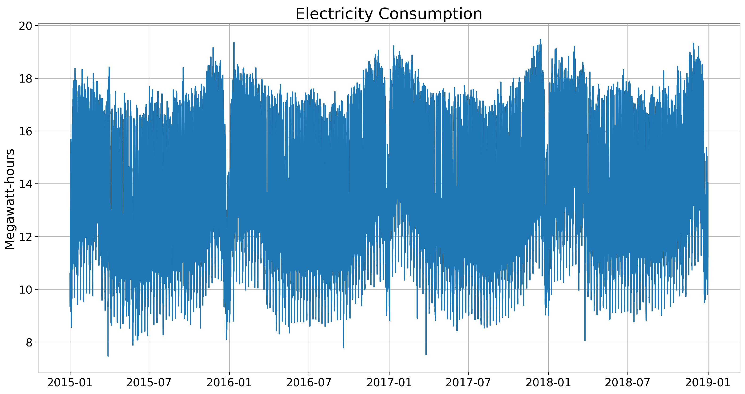
For this study, four years of 15 min intraday electricity consumption data in Germany are considered, spanning from 1 January 2015 to 31 December 2018. The data used for training and evaluation are sourced from Smard (https://www.smard.de/home), the German market transparency platform for electricity consumption, and they can be downloaded freely.

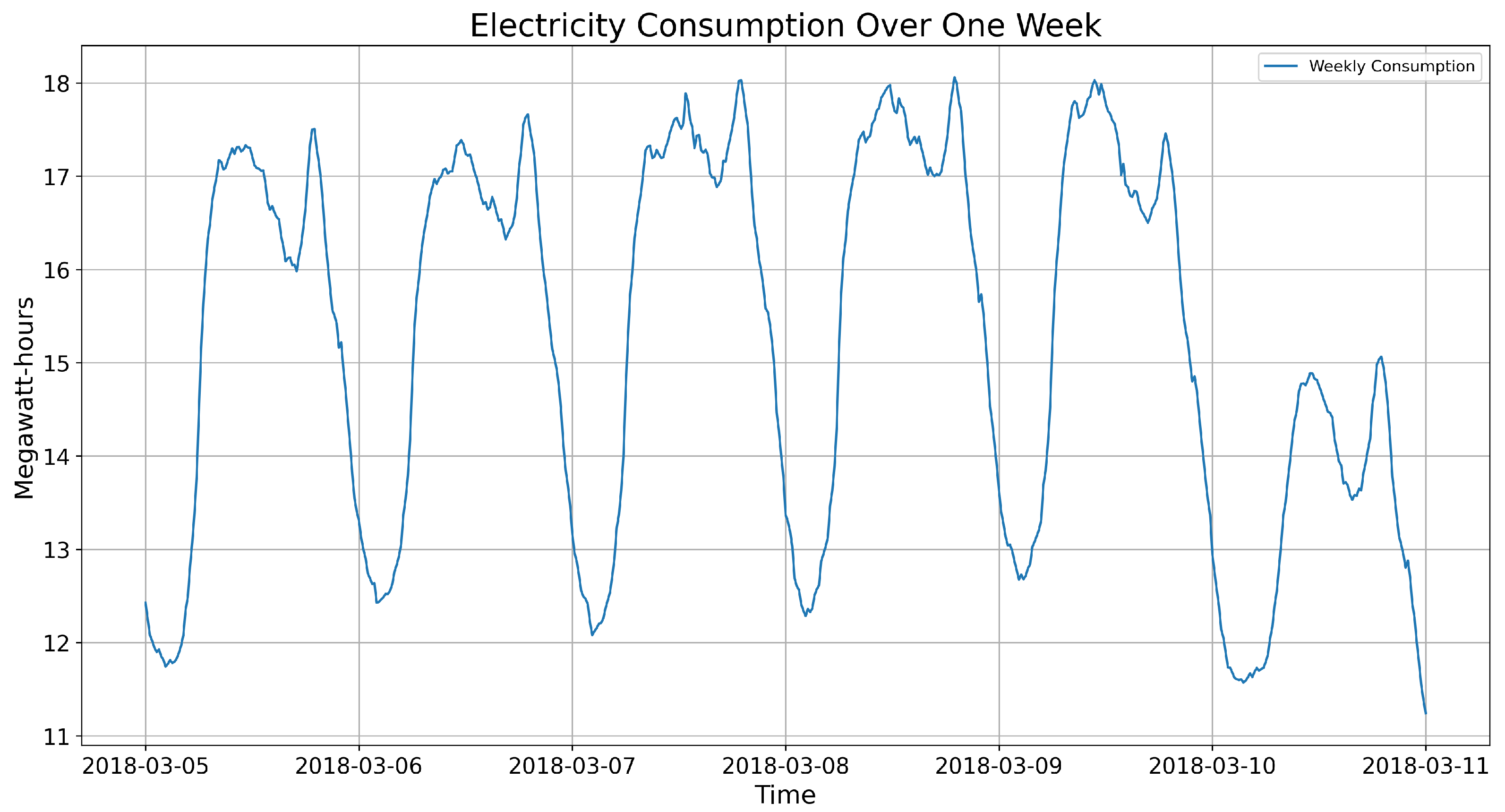
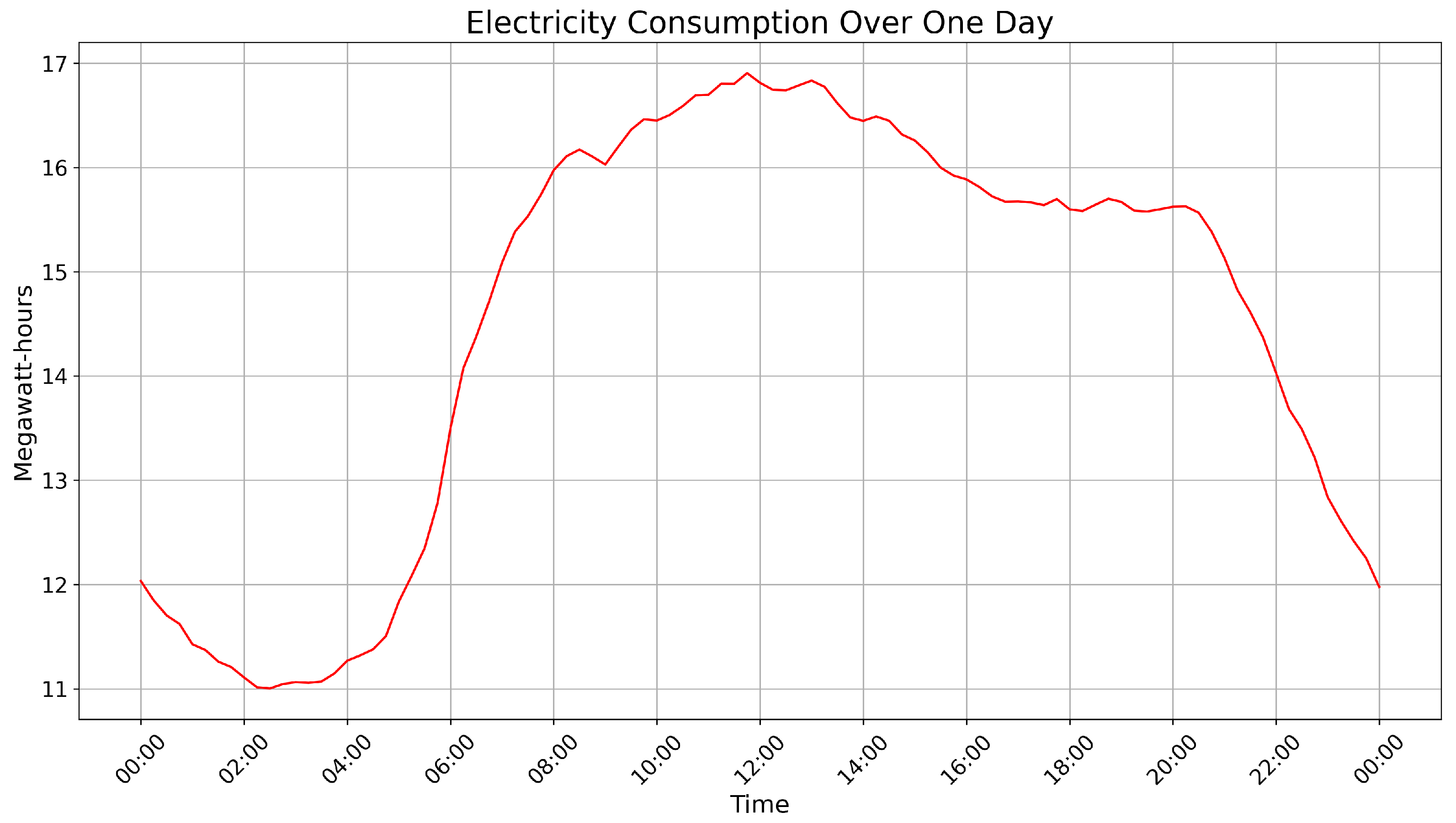
The dataset shows some regularity on a large scale and seemingly random fluctuations on a small scale, as illustrated in Figure 4. Specifically, there is the weekend effect, characterized by lower consumption levels on weekends compared to weekdays (see Figure 5). Additionally, the data display clear seasonal patterns, with consistent daily cycles of electricity usage. For instance, consumption peaks during daytime hours and declines during nighttime, reflecting typical human activity and business operations (see Figure 6). The regularity and seasonality in the data provide a structured framework that ForGAN can leverage to learn and predict the conditional distribution of future consumption effectively.

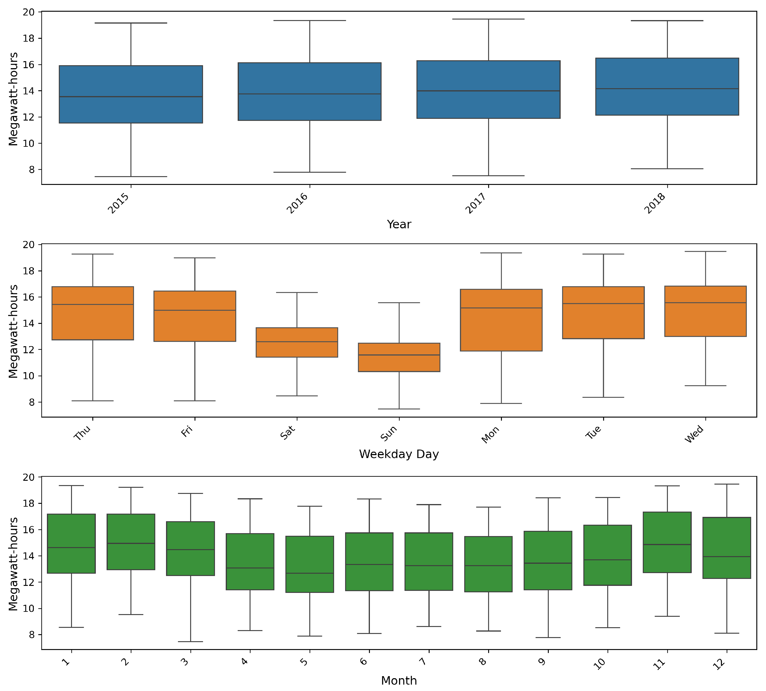
The box plots in Figure 7 highlight the variation in electricity consumption across different time intervals. It is evident from these plots that electricity consumption decreases significantly during weekends and gradually increases over the four-year period. In addition, there is a slight rise in consumption during the winter months, suggesting higher electricity usage for heating purposes. The box plots also show that there are no outliers. This could also be confirmed by using the interquartile range (IQR) method.

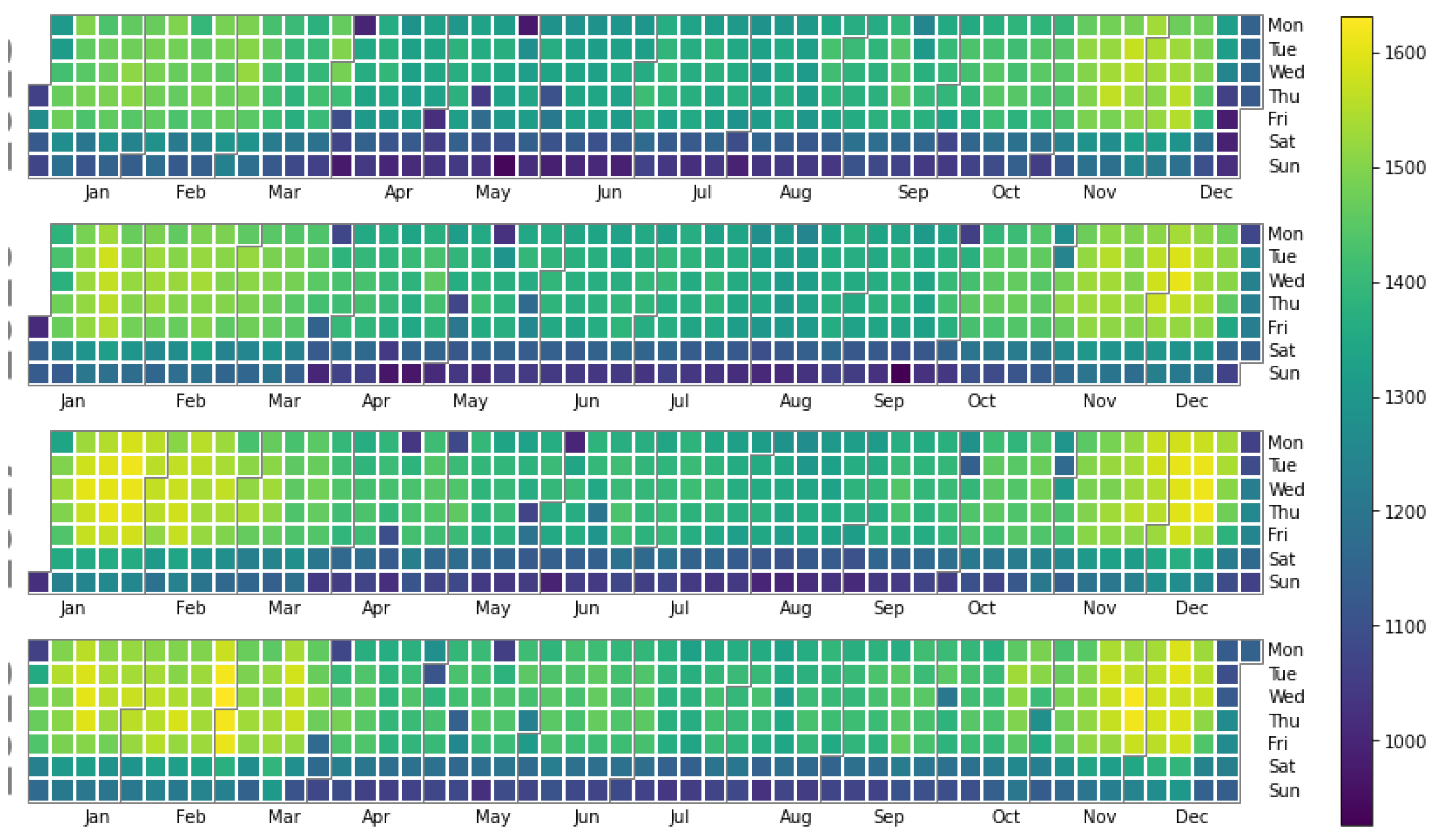
The heatmap in Figure 8 visualizes the daily average 15 min electricity consumption for each day in 2015–2108. The color of each box in the heatmap indicates the height of the consumption, as given by the color bar on the right side of the graph.

The heatmap reveals strong correlations in electricity consumption based on seasonal changes and weekly cycles. These correlations are consistent across the four-year period, although they do not seem to be fully predictable. The absence of significant outliers in the heatmap further suggests stable and reliable data trends. In general, there is a lower correlation between the weekends compared to weekdays across different months. However, this pattern is not uniform, as some months (particularly those with extreme weather conditions) show higher overall consumption, slightly weakening the drop typically seen on weekends. Hence, while weekends generally display lower electricity usage, the amount of this reduction can vary based on the month.

3.2. Hyperparameter Choices and a Priori Decisions for the Application of ForGAN

Various grid searches are performed to make decisions on hyperparameters (i.e., parameters that have to be determined outside the actual algorithm to optimize ForGAN). To explore different hyperparameters (like $windowsize$ for the size of the condition window, $batchsize$ for the size of the batches of real and generated data in training ForGAN, the learning rate in the gradient updates, etc.) across various ranges, other hyperparameters are kept constant. Moreover, the influence of varying one hyperparameter is tested on the performance of ForGAN using a smaller subset of the data.

Some particular hyperparameter choices are

• Size of the condition window: With regard to the size of the condition window (look-back window), it is found that it should be smaller than 200, as a larger size causes memory issues and significantly slows down computations. However, the results are already quite good, with a condition size of 64. A final choice of 96 is used for both the generator and the discriminator, as this also corresponds to a full day of data.
• Number of discriminator gradient descent iterations per generator gradient descent iteration: As already indicated in Section 2.3, different choices for the number k of sequential updates of ${\theta }_D$ before the next update of ${\theta }_G$ are considered. Our experiments led to the choice of $k=2$.
• Number of full iterations of parameter updates: Tests show that the originally intended number of 300 updates is typically too low for the convergence of the generator’s objective function. This number is increased to 1000.
• Choice of the form of the objective function: Again, as indicated in Section 2.3, the non-saturating GAN loss is used as the objective function, i.e., the discriminator maximizes $J_D({\theta }_D;{\theta }_G)$ as given in (2), while the generator maximizes $J_G\left({\theta }_G\right)$ as given in (5).
• Starting the parameter iterations: The parameter search is initialized with ${\theta }_D=0$ and ${\theta }_Q=0$. As this appears to work well and no specific preference exists for alternative starting values, hyperparameter optimization is omitted in this case.

A usually recommended, data transformations do not improve the model. Using the $scaler$ as a hyperparameter shows that scaling the data does not improve prediction accuracy. This result could have been expected, as all box plots show no outliers.

4. Results: ForGAN in Action

ForGAN is applied to the 2015–2018 electricity consumption dataset: parameters are calibrated, validated, and used to generate additional time series, and the performance of ForGAN is evaluated.

In total, there are 140,257 data points. In total, $50\%$ of the data (the first 730 days) are used for training the model. The following $10\%$ (approximately 146 days) are used for validation, and the final $40\%$ are used for testing.

Validation is mainly used to make a decision about the number of iterations to solve the min–max problem corresponding to ForGAN. More precisely, after a certain number of iterations, the currently optimal parameters ${\theta }_G$ are used to generate a path of electricity consumption on the time interval corresponding to the one of the validation set. This generated path is then compared with the validation data (i.e., the actual electricity consumption time series), and quality is assessed visually and through additional measures (see below) to determine whether the generated time series path could be a true one. Once the generated series is deemed satisfactory, the training process is stopped. However, to ensure stability in the parameter estimation sequence, 1000 iterations are ultimately used.

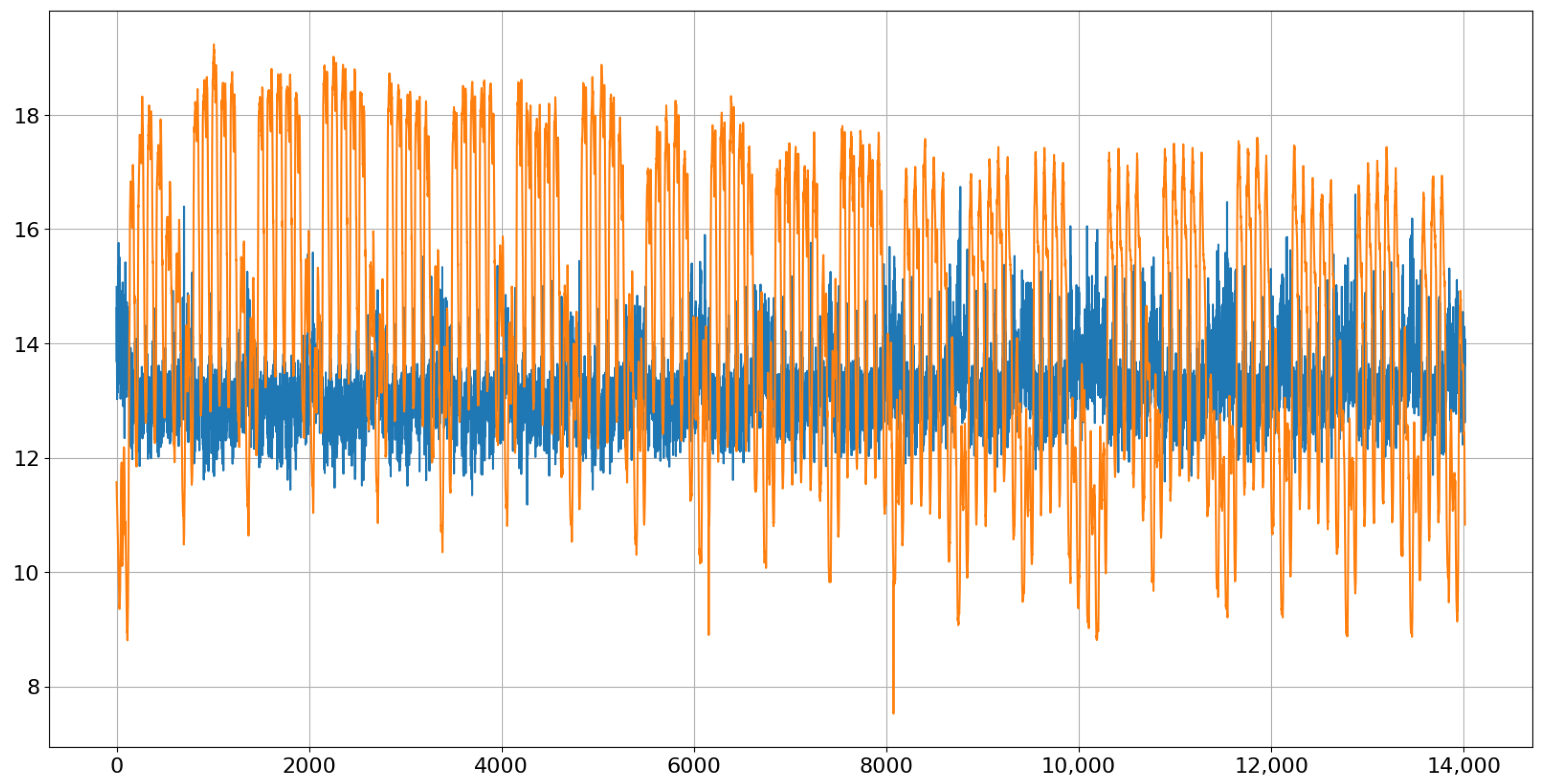
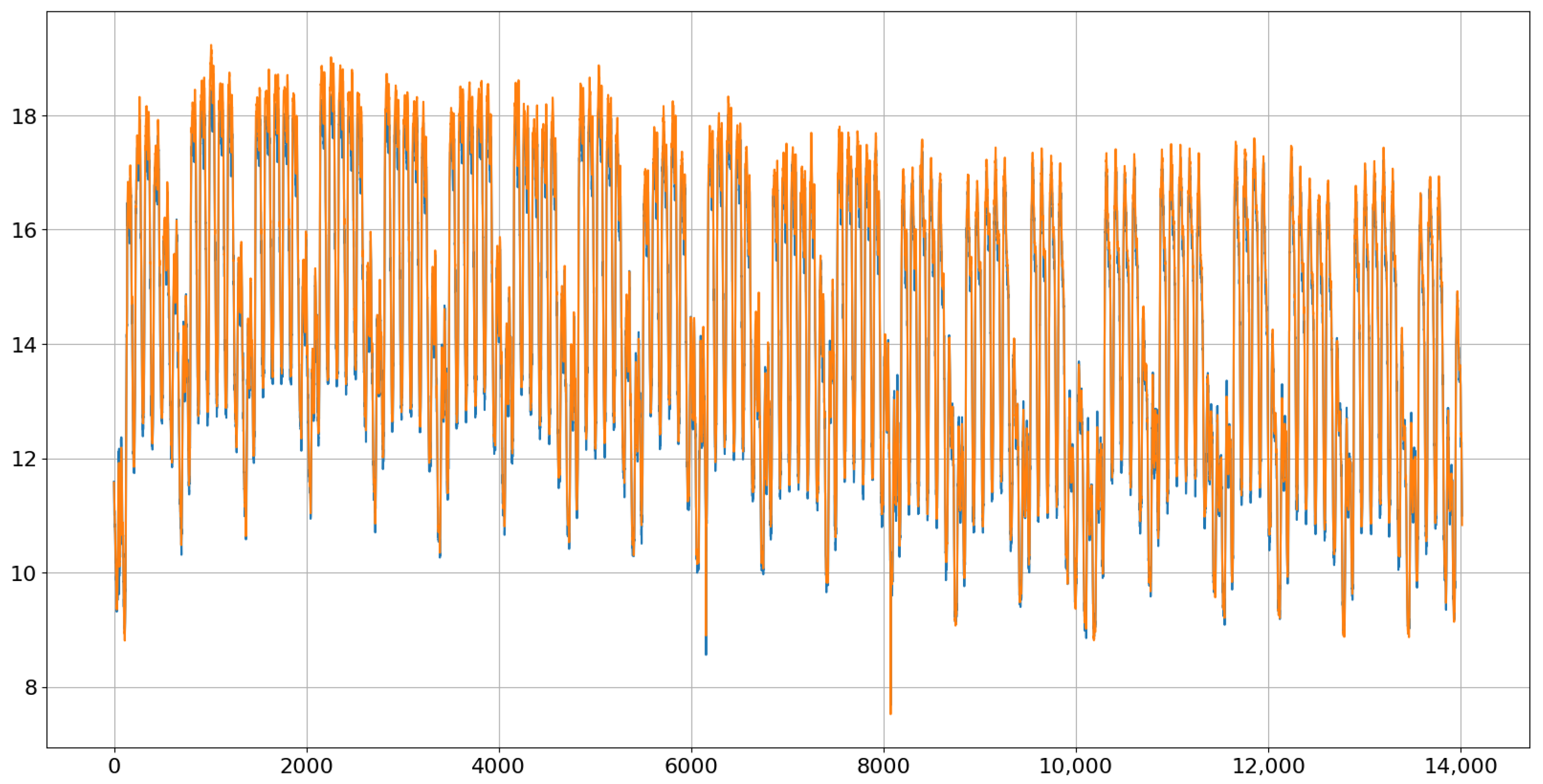
Figure 9 shows the first generated path during the validation process (in blue) together with the times series from the validation set (in red). Obviously, there is room for improvement. Figure 10 shows the last one (in blue) with the final parameter values after 1000 iterations. Indeed, this one follows the actual path (in red) very accurately but is also not identical. The differences that are still visible are a consequence of the randomness in both the red and blue paths. It is important to emphasize that the goal is to learn the conditional distributions of the next value and not to make a perfect prediction.

After having succeeded with implementation and calibration, it is mandatory to perform more quality checks before ForGan can be used for simulation purposes.

The first check is carried out to compute some error and similarity measures. The root mean squared error (RMSE), mean absolute error (MAE) and mean absolute percentage error (MAPE) are calculated based on the error between the predicted and actual values. This is completed by running the generator 100 times over the test set and averaging the values for each run. From this, the mean and standard deviation of these error measures are obtained, as reported in

Table 1. Error metrics used to judge the closeness of the distributions of the 15 min electricity consumption of generated data and the corresponding distribution of the test data.

Metric	Value	Std Dev
RMSE	0.0526	0.000464
MAE	0.0044	0.000532
MAPE	0.00073	0.0041
CRPS	0.0044	-
KLD	0.0072	-

. For additionally judging how close the distribution of the generated data is to the distribution of the values in the test set, the Kullback–Leibler divergence (KLD) and the continuous ranked probability score (CRPS) are also calculated. Notably, a very low KLD value of $0.007154$ is obtained, indicating that the distributions of the test data and the generated data are indeed very close. Also, the small values of the other measures in Table 1 indicate that ForGAN performs well.

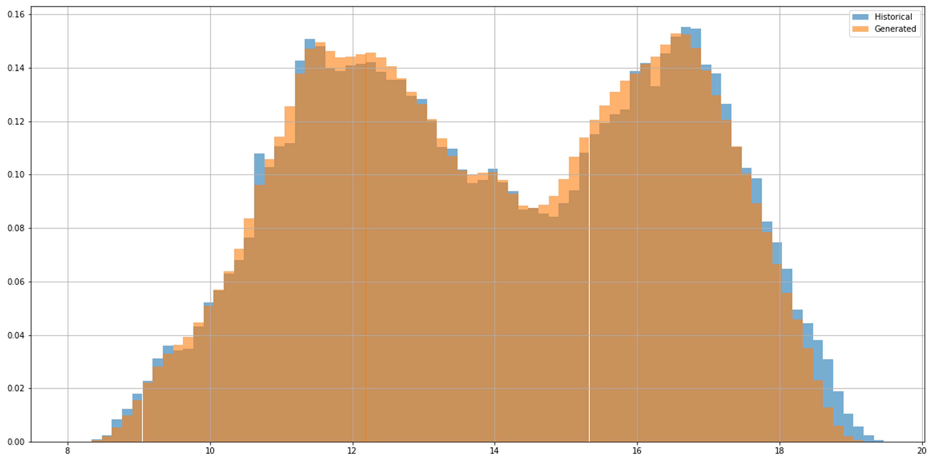
The evaluation plot presented in Figure 11 shows the model’s performance, which is very good. The generated data’s probability distribution for one-step-ahead forecasts captures the original distribution pattern very well when compared to the test dataset. Notably, a bi-modal distribution is present.

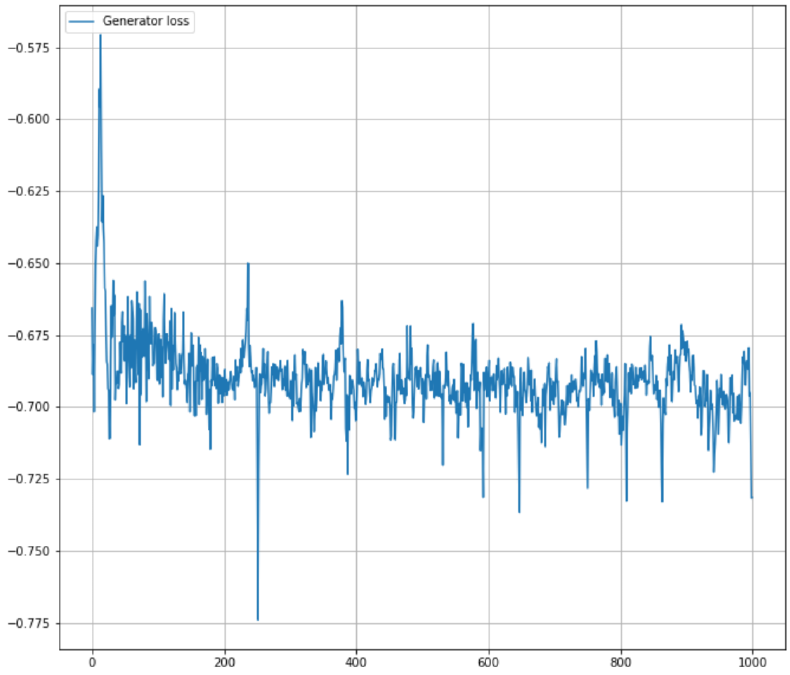
Next, the evolution of the discriminator’s and the generator’s objective functions, $J_D$ and $J_G$, is examined during the training process, as shown in Figure 12 and Figure 13. Note that in the best-case scenario, the setup corresponds to a zero-sum game, and the equality

$$J_D({\theta }_D^{*};{\theta }_G^{*})+J_G\left({\theta }_G^{*}\right)=0$$

(8)

holds.

As the non-saturating GAN loss is used, i.e., the discriminator aims to maximize the (average) sum of the log probabilities for correctly classifying real data and rejecting fake data, meaning that $logD\left(x\right)+log(1-D(G\left(z\right)\left)\right)$, the generator strives to maximize the (average) $log\left(D\right(G\left(z\right)\left)\right)$. To formalize the min-max game, the generator’s loss is multiplied by $-1$.

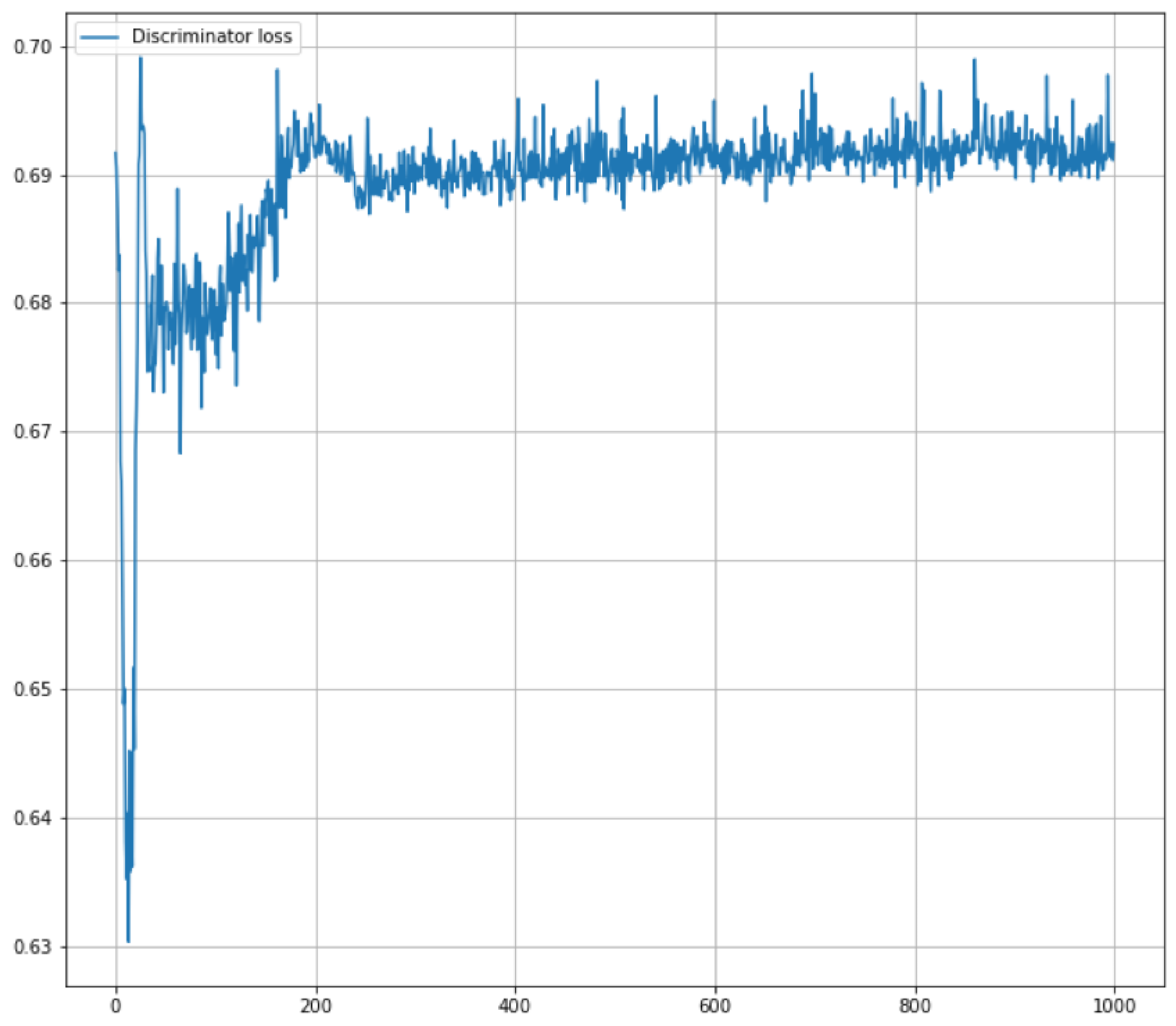
The networks are trained with a non-saturating loss function for 1000 steps. After 200 iterations, the discriminator’s objective function stabilizes, with values fluctuating mostly between 0.69 and 0.70. In contrast, the generator’s loss exhibits larger fluctuations early on but begins to stabilize after 300 training steps, and Equation (8) is close to being satisfactory. This indicates that the found $\theta$-parameters are close to the optimal ones, at least with regard to the requirement of Equation (8).

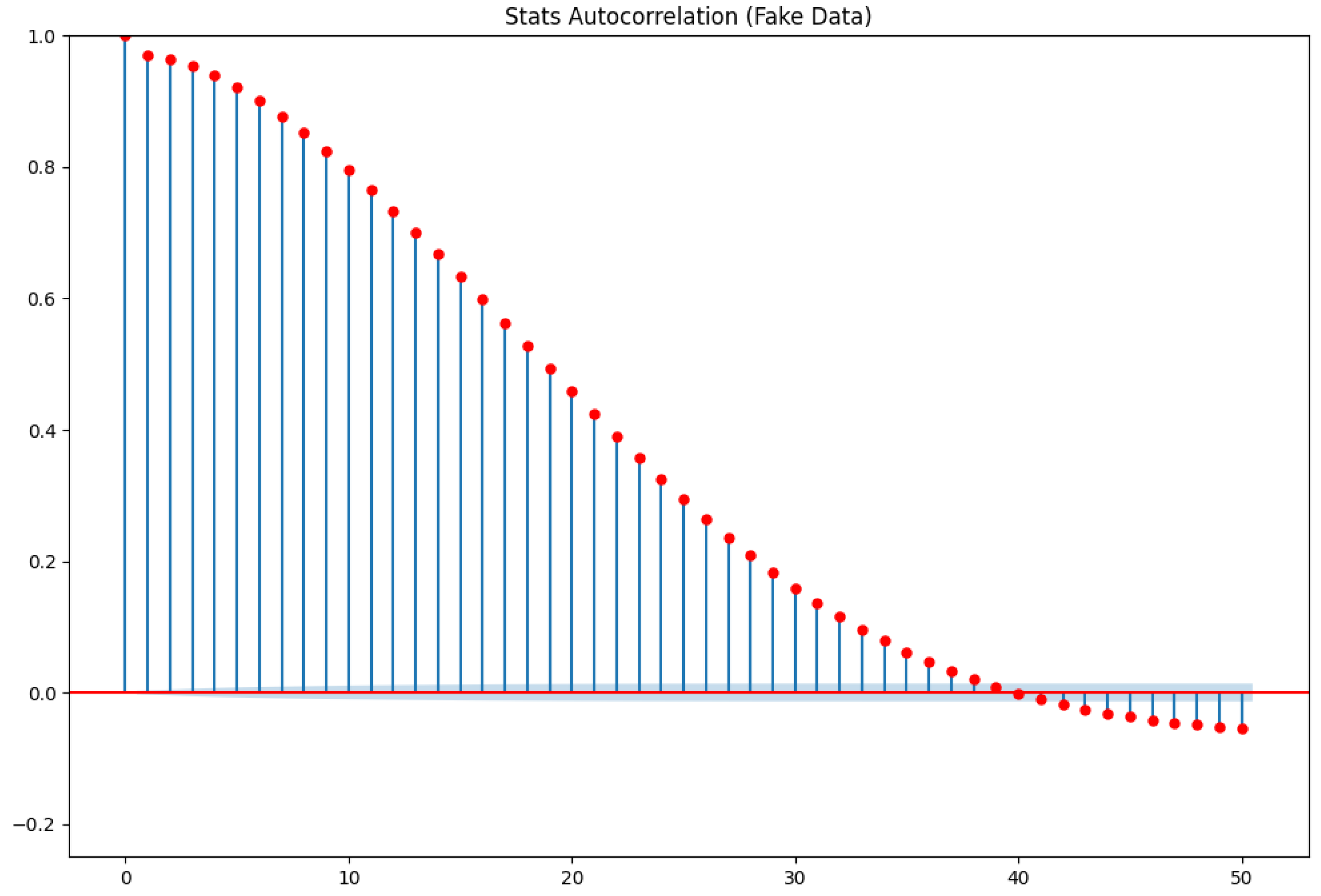
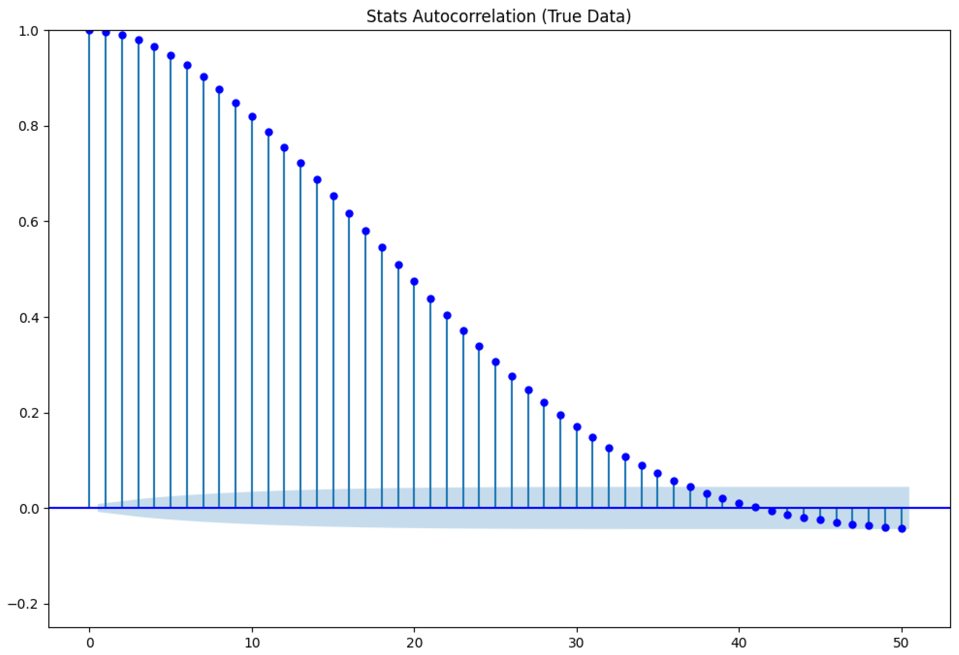
In the next step of the quality check, the auto-correlation plot of the test data series is compared with that of the generated data, i.e., the correlations between the elements $X_j$ and $X_{j+k}$ for $k=0,\dots ,n$ are plotted to examine the influence of previous observations on subsequent ones. The auto-correlation can be seen as a description of the flow of information through a time series.

To generate the auto-correlation plots in Figure 14 and Figure 15, a random consecutive segment of 400 data points is selected from the test and generated data. Using the complete test dataset, which contains 56,096 data points in total, would result in a very fuzzy plot, as will become evident later when the cross-correlation plot of the full time series is considered in Figure 16.

The two graphs show the impressive dependence between the consecutive variables in both time series. Additionally, the shapes of the plots are very similar. Only the lags around 40–50 in the test data seem to have no significant value (as they are inside the blue shadow around the x-axis), although they seem to be significantly correlated for generated data. Still, the difference in the values is small, and the global picture with regard to auto-correlation seems to be well learned by ForGAN.

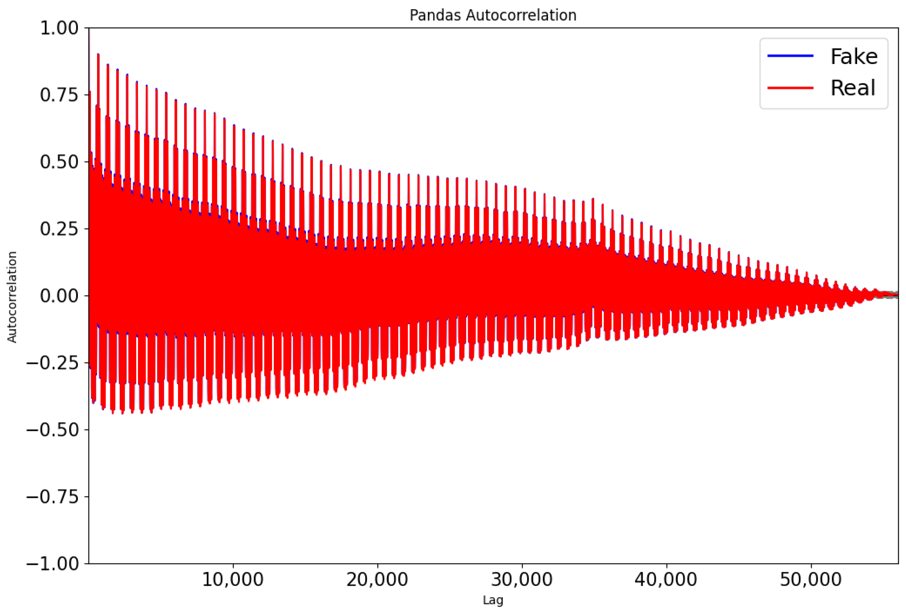
An auto-correlation plot for both the test series and a generated series over all possible lags in the test data is shown in Figure 16. It might look chaotic but it also shows that there are daily and weekly cycles in the auto-correlation that indeed can be observed by the (very many) peaks (keeping in mind that one day has 96 possible lags and a week has 672 lags) and that vanish slowly. These patterns appear to be well learned by ForGAN.

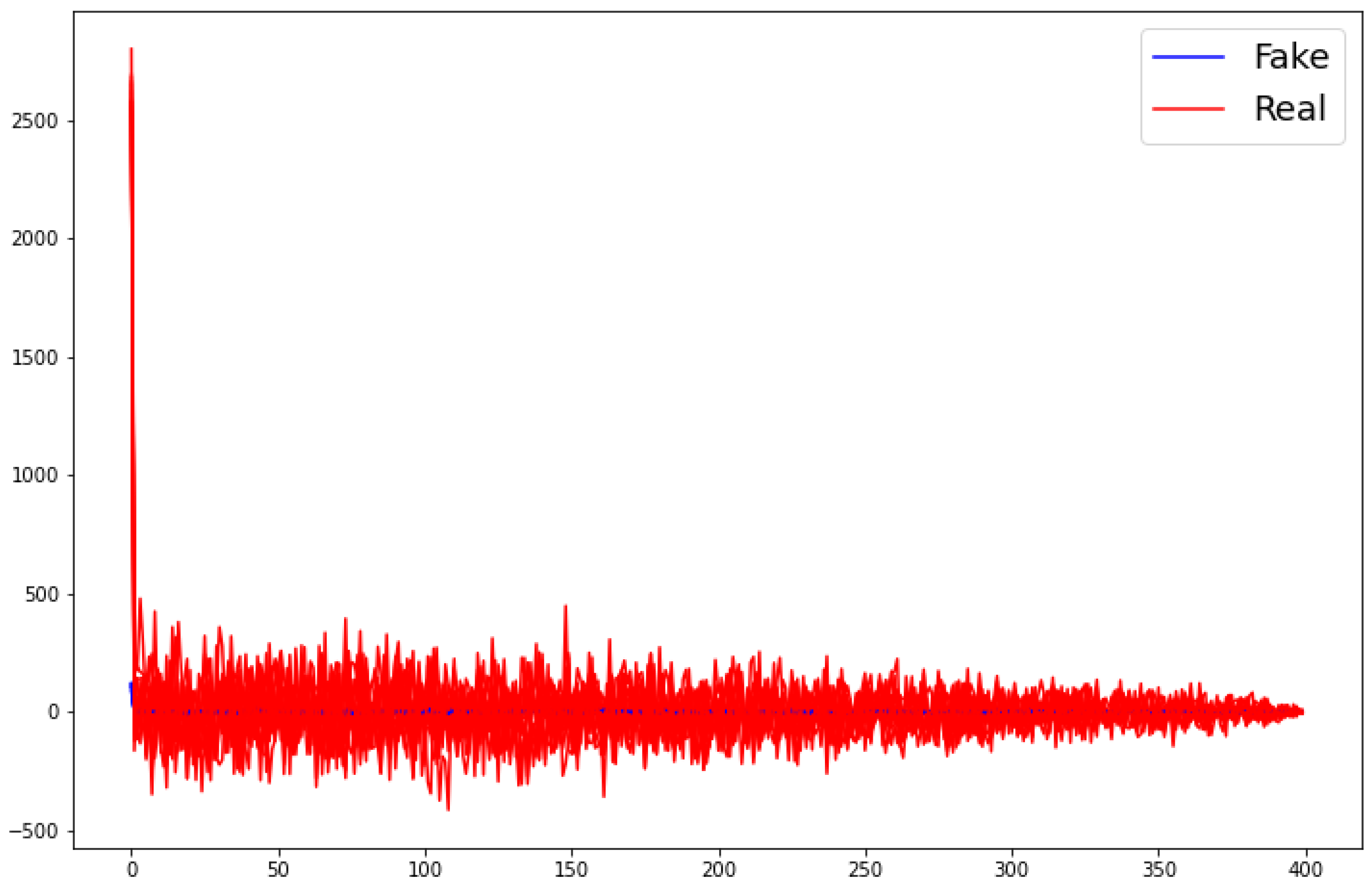
Finally, a test is conducted to determine whether the generated and real time series differ over time by examining their cross-correlation. That is, the analysis checks whether past values of one time series can be used to predict present values of the other. A cross-correlation plot represents frequencies, showing the similarity between signals as a function of the time lag. The cross-correlation plot shown in Figure 17 indicates that the best values of the real time series for predicting today’s value of the 10 randomly generated paths are, in fact, the values from the same day of the real time series. Hence, the true and generated time series evolve in parallel over time.

Due to the fact that we centered and scaled the data before producing the cross-correlation plot, Figure 17 also shows that the generated data closely follow the mean and variance of the real data throughout the time steps. Moreover—as already said above—all time series are highly correlated at the start, diminishing quickly over the time lags.

5. Discussion—Simulating Electricity Consumption with ForGAN

The simulation of additional time series data can help in making a strategic decision as it may reveal phenomena not observed in the historical data. In the case of the electricity consumption example, information of interest might encompass maximum consumption at a particular time (relevant for planning of additional generation capacity), the maximum increase/decrease between two 15 min slots (relevant for transmission stability), and further statistics. This is a feature that the best traditional prediction methods are lacking.

A good and reliable simulation tool for generating such additional time series realizations is thus of big importance. GANs are suggested nearly everywhere today when data are needed. However, naively using some GAN implementations might lead to poor simulation results. In this context, applying a standard GAN without a data preparation step carried out by the GRU or LSTM would cause complete failure, as it ignores the sequential dependence inside the time series.

An essential feature of an application of GANs is a detailed quality check of newly generated data. Therefore, various criteria and methods are presented that should be considered for judging newly generated time series data, such as the following:

• Visual checks such as a comparison of simulated time series’ and the original time series’ graphs on the time interval of the test set.
• Comparison of the auto-correlation structure of the generated time series and the original time series.
• Comparison of the one-step transition probability distribution via histograms and via similarity measures, such as the Kullback–Leibler divergence or the continuous ranked probability score.
• Looking at the generator’s and discriminator’s value of separate objective functions’ sum to see if it is close to zero.
• Looking at the generator’s and the discriminator’s convergence behavior of separate objective functions as the iteration steps’ sequence in the solution of the min–max problem.

Further, as GANs are heavy with regard to computing time, a careful choice and analysis of the hyperparameters is important and has to be carried out before calibrating the internal parameters of a GAN. One should also consider if the use of an LSTM or GRU could be avoided. In [19], a specifically adjusted temporal convolutional network is used for both the representation of the correlation structure in time and the structure of the generator. This network outperformed the LSTM. However, such an additional construction for learning the dependence of the simulation value from its past history is an additional task that is not easy to tackle. Using current laptops, the training of ForGAN is the most time-consuming part, typically taking several hours per configuration. This duration is heavily influenced by hyperparameters such as batch size, number of training iterations, condition size, and learning rate. In contrast, testing and validation are faster, usually taking just a few minutes per configuration, as no optimization is involved.

6. Conclusions

The aim of this paper was to demonstrate the application of ForGAN for simulating additional time series data using a purely data-based approach. To achieve this, every step in the application of ForGAN was considered, from data preparation with advanced but, in principle, ready-to-use tools such as LSTM or GRU via calibration, testing, and validating the model up until its application in data generation.

A reason for the mathematical basics utilized behind GANs and a heuristic description of the general working principle of GANs were also provided.

Further, the differences of classical time series or regression models with regard to obtaining the best prediction of the next value were emphasized. Although such models may also attempt to simulate the conditional distribution of the next value of a time series, they are typically limited to the distribution of this task’s prediction error. Indeed, this is rarely the appropriate distribution.

Key Findings. This study showed that ForGAN can learn and replicate the full conditional distribution of future values in electricity consumption time series. The generated data exhibited strong similarity to real data in terms of distributional characteristics, auto-correlation structures, and cross-correlation dynamics—making ForGAN a valuable tool for simulating realistic future scenarios.

It is hoped that this paper will help to demystify GANs and encourage their recognition as a useful tool for data simulations that has to be handled with care.

Future Research Directions. Potential extensions of this work include applying ForGAN to multivariate time series involving electricity consumption, prices, and weather variables. Additionally, integrating ForGAN into real-time decision-making systems or comparing it with other generative frameworks such as TimeGAN or diffusion models could offer further insights into the practical capabilities of ForGAN.

Implications. Researchers in the area of electricity production, consumption, and capacity planning are encouraged to base decisions on the full distribution of the resulting future data, generated using ForGAN, before implementing actual strategies.