Optimized Active Learning Method for High-Dimensional Industrial Regression Problems

Abstract

Machine learning approaches are commonly used to model physical phenomena due to their adaptability to complex systems. In general, a substantial number of samples must be collected to create a model with reliable results. However, collecting numerous data points is often costly. Moreover, high-dimensional problems inherently require large amounts of data due to the curse of dimensionality. That is why new approaches based on smart sampling techniques are being investigated to optimize the acquisition of training samples, such as active learning methods. Initialization is a crucial step in active learning as it influences both performance and computational cost. Moreover, the scenarios used to select the next sample, such as classic pool-based sampling, can be highly resource- and time consuming. This study focuses on optimizing active learning methods through a comprehensive analysis of initialization strategies and scenario design, proposing and evaluating multiple approaches to determine the optimal configurations. The methods are applied to high-dimensional industrial problems with dimensions ranging from 5 to 15, where challenges associated with high dimensionality are already significant. To address this, the proposed study uses an active learning criterion that combines Sparse Proper Generalized Decomposition with Fisher information theory, specifically tailored to high-dimensional industrial settings. We illustrate the effectiveness of these techniques through examples on theoretical 5D and 15D functions, as well as a practical industrial crash simulation application.

1. Introduction

Machine learning [1] is now commonly used to tackle industrial problems efficiently, saving both time and cost. Indeed, machine learning makes it possible to estimate an output value $\mathit{y}$ based on multiple input variables $\mathit{x}=(x_1,\dots ,x_n)$. To do so, a statistical model is trained on a subset of examples $\xi$ and can then make predictions for unseen examples. The choice of training database significantly impacts the algorithm’s performance and the accuracy of predictions. Given the high cost of generating training samples, careful selection is crucial, especially considering the “curse of dimensionality” [2] that arises in complex problems involving multiple input parameters. This implies that, as the number of parameters increases, the number of sampling points needed for proper exploration grows exponentially.

Traditionally, training databases are built using Design of Experiments [3], but active learning has now emerged as an alternative approach. Active learning  [4] is an iterative technique where the training database is built along with the model. At each iteration, the sample expected to provide the highest improvement in the overall performance is selected. To assess a sample’s potential, various information criteria have been developed, but many are limited in high-dimensional settings.

Moreover, in active learning, there are different scenarios defining how to select and add a new sample to the training database. The three main settings considered in the literature are (i) membership query synthesis [5,6,7], (ii) stream-based selective sampling [8], and (iii) pool-based sampling [9]. The most common one is pool-based sampling, where a small set L of labeled data and a large set denoted U of unlabeled available data are considered. A new sample is chosen using an information criterion that measures how relevant a sample from the basis U is compared to the others. The sample with the highest score is added to the training set. However, since the criterion must be calculated for every sample in U, this approach can be very costly.

Active learning strategies aim to create or reinforce databases using an adaptive model. This raises the fundamental problem of model initialization [10,11,12,13,14], yet few studies address how to choose the initial samples effectively. Most studies assume that the initial training set is provided and focus on the active learning phase even though the overall process is strongly dependent on the initialization process. As this choice remains uncertain, multiple runs are needed to obtain reliable results, inevitably increasing computational expenses.

As a result, optimized methods should be implemented to address these issues.

As the focus of this study is a high-dimensional industrial regression problem, we selected a criterion that has demonstrated effectiveness in such contexts to focus on the initialization and scenarios. In [15], a corresponding criterion was proposed. It uses an information criterion from a combination of the information provided by Fisher [16] with a Sparse Proper Generalized Decomposition (s-PGD) [17], showing efficient results where classic active learning approaches, such as Gaussian processes, fail because of the dimensionality. Indeed, in this criterion, the use of s-PGD enables a separation of variables, which is particularly efficient in high dimensions. Here, we aim to study the impact of initialization on the active learning process, make optimal selections, and develop an efficient scenario, such as a surrogate, derivative, or mathematical optimization approach. The current study is developed for this criterion but could be extended to others, especially variance-based ones. In this article, we present in Section 2 the context of active learning and provide some insight into the criterion. In Section 3, different scenarios are proposed, including mathematical, derivative, and surrogate approaches, and tested. Then, Section 4 involves an in-depth study of the initialization and its impact on active learning performance. In Section 5, the resulting methodology is applied to an industrial crash simulation problem. Finally, the article is completed with a discussion.

The novelty of this article lies in studying initialization and its impact on active learning, along with the proposition of new scenarios, especially in industrial high-dimensional contexts. This ultimately results in a novel optimized active learning methodology designed for high-dimensional industrial problems. The study aims to open doors for the optimization of initialization and scenario design in active learning in general.

2. Background and Review

2.1. Active Learning

First, existing work on active learning is reviewed. In the field of machine learning [1], statistical algorithms are developed to learn from data and generalize to unseen data. For example, there are Decision Tree or k-Nearest Neighbor [18] for classification problems or Gaussian process [19], SVM [20], etc., for regression problems. In this context, it is necessary to select samples to form a training database to fit the models, which has been completed through Design of Experiments [3]. Static methods such as Full Design [21], Factorial Design [22], Latin hypercube sampling (LHS) [23], and Plackett–Burman [24] were applied to form an a priori list of samples that compound the training database. More recently, other approaches have been developed with the rise of active learning. In these methods, the training database is incrementally constructed alongside the model by adding, at each step, the sample that maximally improves performance. This “best” sample is determined according to an information criterion. The literature offers multiple definitions, including uncertainty sampling [9,25,26], expected model change [27,28], and variance reduction [29], among others. Most of these criteria are based on the posterior distribution’s probability to quantify the information of a sample, which can also be extended to regression models. The most famous example can be found in Gaussian processes, where the variance is used as an information-measuring unit [29]. However, most of these criteria are not well suited for high-dimensional problems. In particular, many of them rely on distance-based definitions in the input parameter space, which become inefficient as dimensionality increases.

2.2. Considered Information Criterion

For this reason, Ref. [15] introduced an information criterion specifically designed for high-dimensional industrial problems. This criterion combines Sparse Proper Generalized Decomposition (s-PGD) [17] with Fisher’s information. This criterion was selected because it has proven to be efficient in high-dimensional industrial contexts. Indeed, the use of s-PGD enables a separation of variables, making it particularly effective in such high-dimensional settings. A brief summary of its definition is presented below, while a more detailed discussion can be found in the referenced article.

In an n dimensional space, on a considered point $\mathit{x}=(x_1,x_2,\dots ,x_n)$ and for a model previously trained on the database $\xi$, this criterion is defined as the following function:

$$d(\mathit{x},\xi ):{\mathbf{R}}^n\to \mathbf{R}.$$

(1)

$$\begin{array}{c}\hfill d(\mathit{x},\xi )=J{(\mathit{x},\xi )}^{T}I(\mathit{x},\xi )J(\mathit{x},\xi ).\end{array}$$

(2)

where

$$J(\mathit{x},\xi )=\left({\displaystyle \frac{\partial f(\mathit{x},\xi )}{\partial \mathit{x}}}\right)$$

(3)

and

$$\begin{array}{cc}\hfill I\left(\mathit{x}\right)& =\mathbb{E}\left(\left({\displaystyle \frac{\frac{\partial f(\mathit{x},\xi )}{\partial \mathit{x}}}{f(\mathit{x},\xi )}}\right){\left({\displaystyle \frac{\frac{\partial f(\mathit{x},\xi )}{\partial \mathit{x}}}{f(\mathit{x},\xi )}}\right)}^T\right)\hfill \end{array}$$

(4)

In this formulation, $f(\mathit{x},\xi )$ represents the s-PGD regression approximation of the target function, expressed as a combination of polynomial functions.

Evaluating the criterion function $d(\mathit{x},\xi )$ at a point in the parametric space yields a value d, which serves as an information criterion within the active learning process. As it originates from Fisher’s definition, d is analogous to a variance, with higher values indicating areas of greater interest. This criterion thus facilitates the identification of informative areas in the parametric space where additional data should be acquired.

As demonstrated in [15] for a pool-based scenario, this criterion performs particularly well in high-dimensional industrial settings, which justifies the choice of this particular criterion for the present study conducted within the same framework. However, pool-based scenarios are associated with significant computational costs.

3. Numerical Optimization

The pool-based scenario is the most commonly used approach in active learning despite being computationally intensive and time-consuming. This motivates the evaluation of more optimized strategies.

3.1. The 5D Results

3.1.1. Function

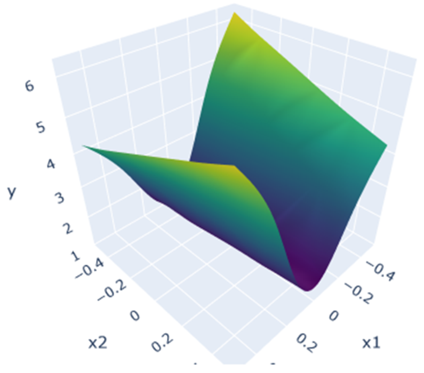
As a first example, we are trying to estimate the following polynomial function defined in Equation (5) from [30] in a 5-dimensional input space. A ground-truth plot of this function is shown in Figure 1.

$$\begin{array}{cc}\hfill f(\mathit{x}& =(x_1,x_2,x_3,x_4,x_5))\hfill \\ \hfill & ={(8x_1^3-6x_1-0.5x_2)}^2+{(4x_3^3-3x_3-0.25x_4)}^2+0.1(2x_5^2-1).\hfill \end{array}$$

(5)

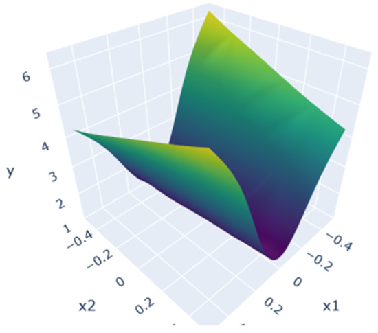
Figure 1. Ground truth for $f(x_1,x_2,x_3=0,x_4=0,x_5=0.7071)$.

The function is defined on the domain $\Omega ={[-0.5,0.5]}^5$, and the predictions are made over this space using an s-PGD model trained with our previous active learning method. For training purposes, the s-PGD hyperparameters (modes and degrees) are chosen to prevent overfitting and ensure good generalization. Features were selected to achieve a training correlation exceeding 0.85. These values are now kept fixed throughout the active process. However, adapting the modes during the process to achieve greater precision would be an optimization worth considering. In this section, the initial training set is an LHS of 25 samples. The process is completed after 30 queries, once convergence of the active learning procedure is achieved. This value was chosen from preliminary tests to provide a compromise between computational cost and convergence.

To obtain a direct comparison of the performance of each method, the correlation coefficients, defined in Equation (6) and calculated on a test set, are evaluated. The coefficient of determination was chosen as the performance metric because it provides a straightforward and widely used measure of how well the model predictions match the reference data, making it suitable for comparing the accuracy of different active learning strategies.

$$R^2={\displaystyle \frac{{\sum }_{i=1}^n({\mathit{y}}_{pred,i}-\overline{{\mathit{y}}_{pred}})({\mathit{y}}_{true,i}-\overline{{\mathit{y}}_{true}})}{\sqrt{{\sum }_{i=1}^n{({\mathit{y}}_{pred,i}-\overline{{\mathit{y}}_{pred}})}^2}\sqrt{{({\mathit{y}}_{true,i}-\overline{{\mathit{y}}_{true}})}^2}}},$$

(6)

where ${\mathit{y}}_{pred}$ corresponds to the prediction made by the model, ${\mathit{y}}_{true}$ to the real output values, and $\overline{{\mathit{y}}_{pred}}$, $\overline{{\mathit{y}}_{true}}$ to the corresponding means.

3.1.2. Pool-Based Sampling

In the original methodology [15], a pool-based scenario was employed, meaning that the next sample is selected from a pool of available unlabeled points. This pool is constructed as a k-dimensional research grid with N subdivisions per dimension, resulting in $N^k$ evenly distributed candidate samples across the input parametric space. Here, a refined grid of size ${20}^5$ is used to provide a wide range of query options. The information criterion is computed for each sample in the pool, and the sample with the highest criterion value is selected. Its true output is then evaluated and added to the training set. This methodology is detailed in Algorithm 1.

Algorithm 1 Scenario: Pool-Based

1: Initialization   2: Define a training set $\xi$ for the learner   3: Train the learner on $\xi$   4: Main   5: while Stopping condition not reached do   6:     Apply the criterion function all over the pool   7:     Determine best element (i.e., the maximum)   8:     Add the best element to $\xi$   9:     Train the learner on the new $\xi$ 10: end while

In this case, the test set consists of all points in the pool that are not used for training. Since the pool forms a refined grid, it is assumed to be densely populated and evenly distributed, providing reliable evaluation results. This test set will be used for the purpose of this study as a whole.

However, computing the criterion across the entire pool to select the maximum is inefficient as it requires many unnecessary calculations.

3.1.3. Mathematical Optimization

A first option to improve this process is to apply well-known mathematical optimization functions to find the maximum value more efficiently. The methodologies considered are as follows:

• Nelder–Mead: The Nelder–Mead method is a heuristic optimization method for finding the minimum of a function in a multidimensional space by iteratively adjusting a simplex [31,32].
• L-BFGS-B: The L-BFGS-B (limited-memory Broyden–Fletcher–Goldfarb–Shannon) is a limited-memory quasi-Newton optimization algorithm used for solving large-scale nonlinear optimization problems with bounds on the variables. In this study, we use the L-BFGS-B algorithm defined in [33,34].
• SLSQP: The SLSQP (Sequential Least Squares Quadratic Programming) method is an iterative optimization algorithm for solving constrained nonlinear optimization problems. The method, in this study, wraps the SLSQP optimization subroutine originally implemented by Dieter Kraft [35].

This leads to the methodology in Algorithm 2:

Algorithm 2 Scenario: Mathematical Optimization

1: Initialization   2: Define a training set $\xi$ for the learner   3: Train the learner on $\xi$   4: Main   5: while Stopping condition not reached do   6:     Determine the maximum of the criterion function using an optimization algorithm   7:     Add the corresponding best element to $\xi$   8:     Train the learner on the new $\xi$   9: end while

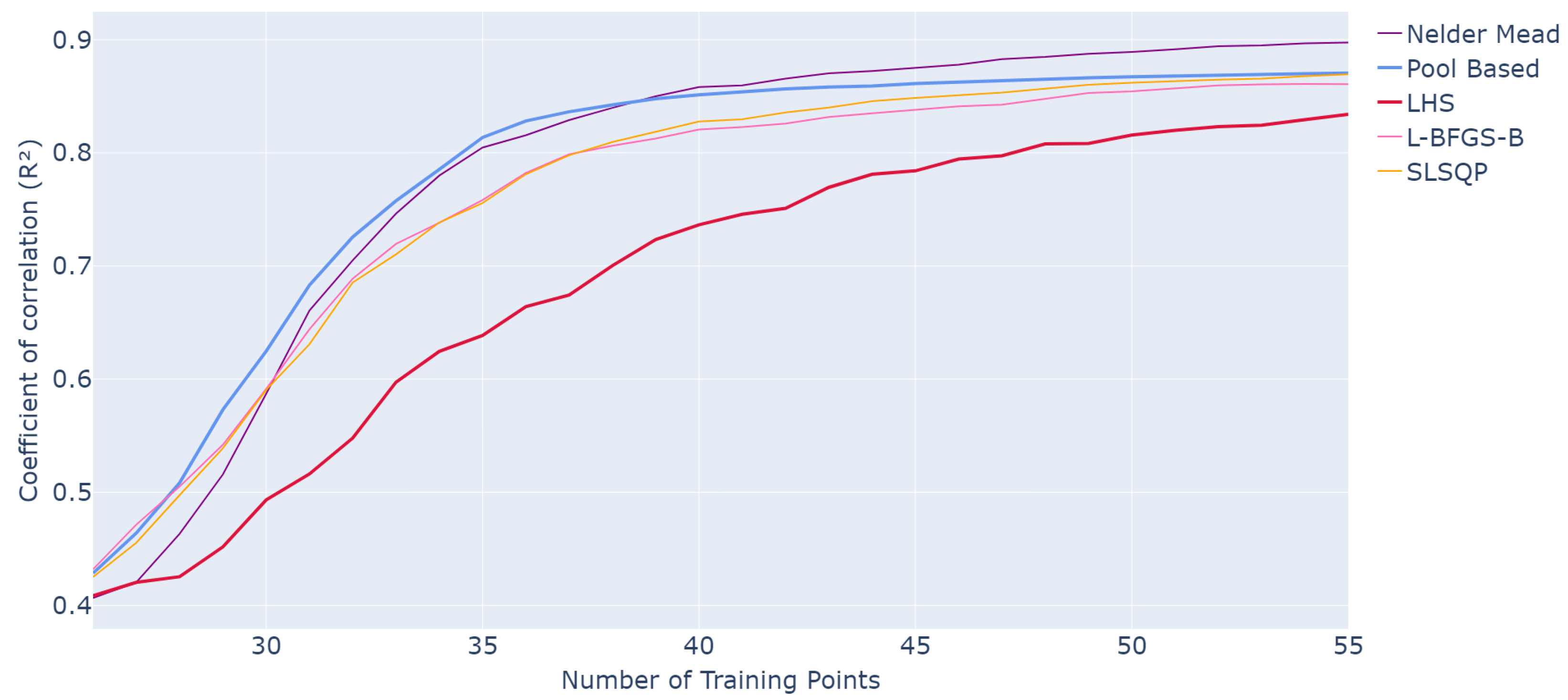
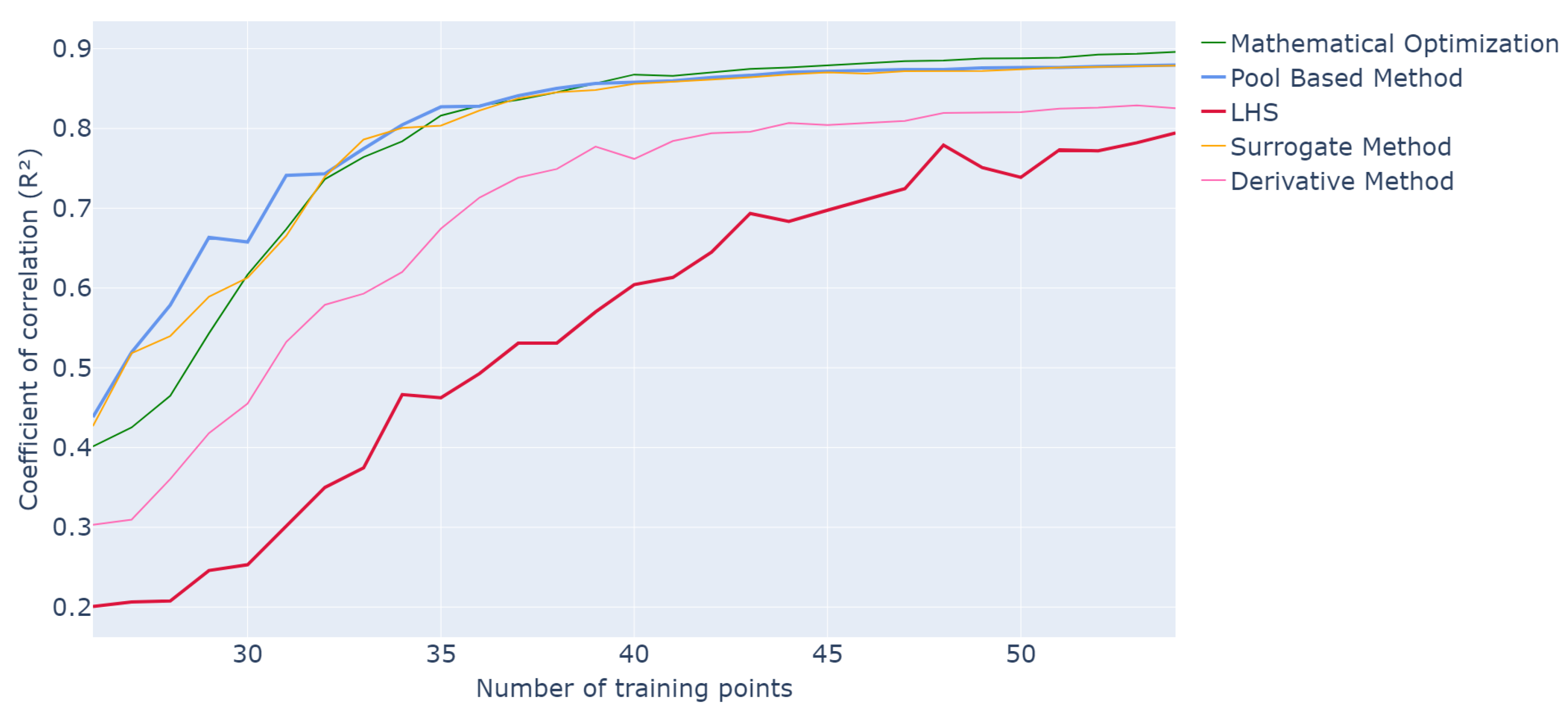
The results of the different methods are shown in Figure 2. Each curve corresponds to the application of the scenario indicated in the legend for selecting the next sample. The LHS curve is included as a baseline to illustrate the performance of standard sampling. Performance is measured using the $R^2$ value on the test set as a function of the number of training samples.

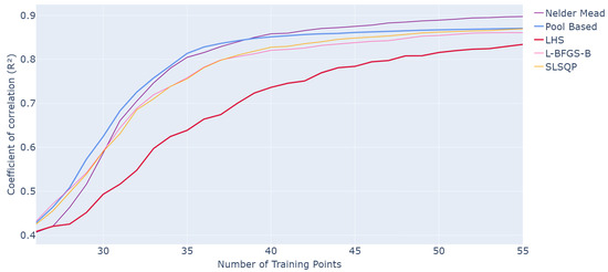
Figure 2. Evolution of R² values for different optimization methods as a function of the number of points in the training set over 50 runs of the whole active learning process.

For the active learning methods, the process is initialized with an LHS of 25 samples. Since this initialization introduces variability in the results, each curve is averaged over 50 independent runs of the complete active learning procedure. For comparison, an s-PGD is trained on an LHS with the same number of samples as the active learning methods at each step. Similarly, the LHS baseline is repeated 50 times, and the average $R^2$ is reported at each step.

These averaged results provide a representative measure of performance while enhancing readability. The variance across the different runs is a point of interest that will be studied more deeply in Section 4 with the study of initialization.

Overall, all methods show an improving trend in predictive performance as more training samples are added, highlighting the benefit of iterative sample enrichment. With active learning methods, a performance of $R^2=0.80$ can be achieved with only 35 training samples compared to $R^2=0.64$ using LHS sampling. Adding points in a smart iterative manner leads to better performance with fewer samples, especially in the early stages before the curves begin to converge. In general, the active learning approach with pool-based sampling consistently outperforms classical LHS.

When considering the optimized scenarios, all methods demonstrate strong average performance, with Nelder–Mead being the most efficient. Its performance is the closest to pool-based sampling, reaching $R^2=0.80$ compared to $R^2=0.81$ for pool-based at 35 samples, and even surpassing it at larger training sizes, achieving $R^2=0.90$ compared to $R^2=0.88$ for pool-based at 55 samples.

The L-BFGS-B and SLSQP methods also demonstrate competitive performance, closely following pool-based sampling throughout the iterations. At 35 samples, both achieve $R^2=0.75$. Their curves remain consistently above the LHS baseline ($R^2=0.64$ at 35 samples), confirming that all active methods outperform classical sampling, with faster gains in predictive accuracy.

Since the aim is to develop a faster methodology, the computational cost was also evaluated. A representative running time was defined. It corresponds to the running time of one iteration of the active learning process (time for one loop in the algorithms). The times were calculated for each iteration and for 50 runs of the whole active process. The results plotted in the histograms correspond to the mean over all the iterations and runs in seconds. All the simulations were performed on servers equipped with 2 × 24-core CPUs (48 cores per node, 2.2–2.9 GHz), 192 GB RAM, and InfiniBand HDR 100 Gb/s interconnects, running Rocky Linux 8.9.

These optimization methods show slightly lower runtimes than the pool-based scenario, although the difference remains relatively minor, as illustrated in Figure 3. This observation encourages the exploration of alternative strategies to further reduce computational cost.

Figure 3. Barplot of the representative computing time in seconds for each method.

3.1.4. Derivative

Another proposition is to use the derivative to find the maximum of the criterion more directly. Indeed, the criterion function is a combination of one-dimensional polynomial functions because it comes from an s-PGD regression. As a polynomial function, the derivative of the criterion can be easily obtained. The Newton Method [36] can then be applied to find the roots. The best sample is associated with a maximum value of the criterion; thus, it also corresponds to a null value of the derivative of the criterion. Therefore, with this method, the sample to add to the training set should be identified faster. In comparison, in pool-based sampling, this criterion function was applied to each sample of the pool to estimate its value, and then the maximum was selected.

The whole process is detailed in Algorithm 3.

Algorithm 3 Scenario: Derivative

1: Initialization   2: Define a training set $\xi$ for the learner   3: Train the learner on $\xi$   4: Main   5: while Stopping condition not reached do   6:     Compute the derivative criterion function   7:     Use an optimization algorithm to find the roots of the derivative   8:     Add the best element to $\xi$   9:     Train the learner on the new $\xi$ 10: end while

However, the best value of the criterion does not always correspond to a null value of the derivative of the criterion. Indeed, the best value of the criterion is often located on the border of the considered space. Thus, the maximum is not a global maximum, and the derivative is not null because we focus on an optimal subspace.

To solve this issue, we added special research on the border if no null value was found. To conduct this specific research, a pool of samples located on the border of the considered subspace is created. The criterion function is applied to each sample of this border pool, and the maximum is selected.

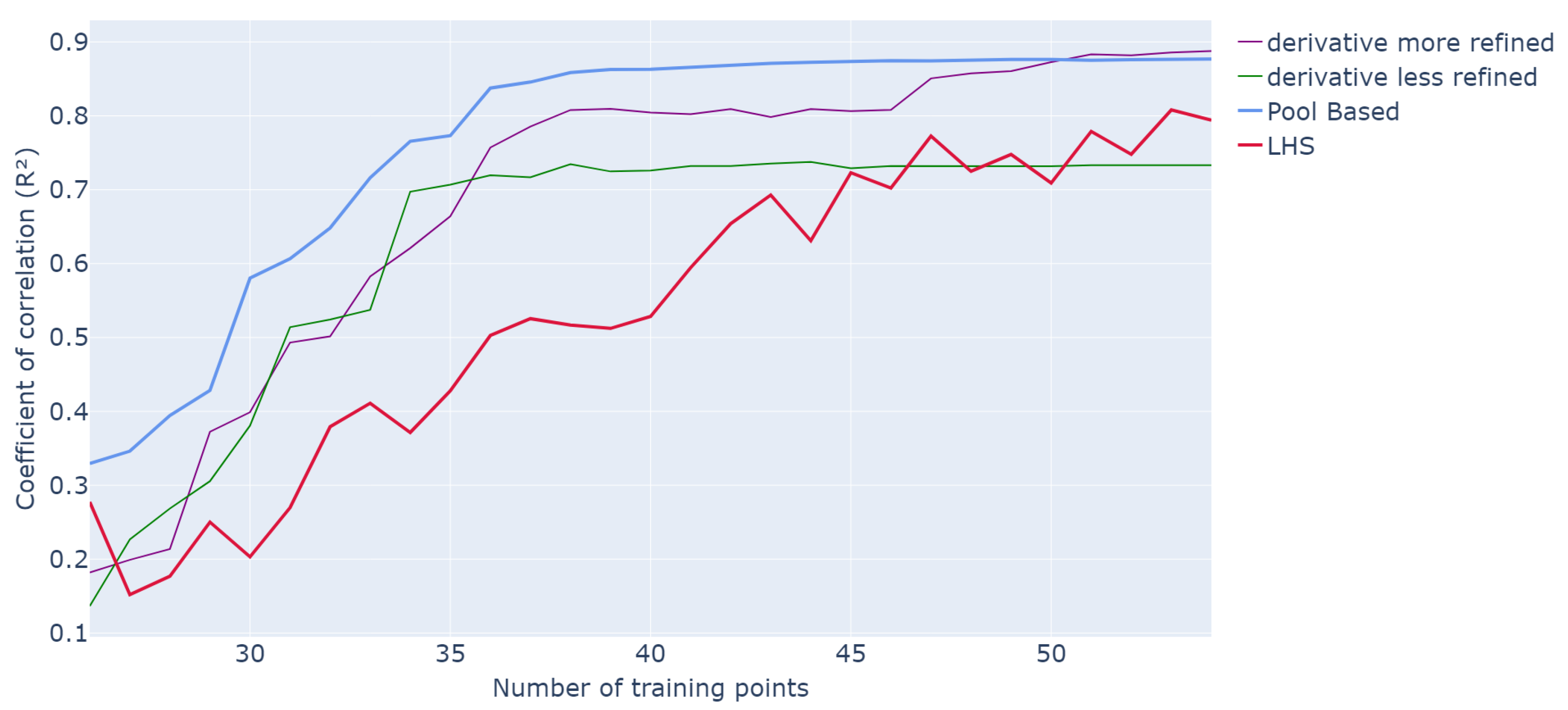
The derivative method is then applied to the same 5-dimensional problem, keeping the same global framework, and the results are shown in Figure 4 and Figure 5. For reference, all methods start with an LHS of 25 samples, the results are averaged over 50 iterations of the whole process, and they are compared to a classical LHS with the same number of samples. The process is stopped after 30 queries, and the s-PGD model is trained as before. The pool is a ${20}^5$ grid. Figure 4 reports the performance in terms of the average $R^2$ as a function of the number of training points, while Figure 5 presents the efficiency in terms of representative computing time. For the border search, both more and less refined pools are considered.

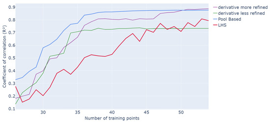
Figure 4. Evolution of R² values for different methods as a function of the number of points in the training set over 20 runs of the whole active learning process.

Figure 5. Barplot of the representative computing time in seconds for each method.

Concerning performance, both derivative methods outperform classic LHS sampling but remain slightly below the pool-based approach. For example, with 35 training points, $R^2$ values of $0.66$ and $0.71$ are achieved for both the more and less refined derivatives compared to $0.77$ and $0.43$ for the pool-based and LHS methods, respectively. The two derivative methods exhibit a steep initial increase in performance, characteristic of active methods, followed by a plateau. As expected, the more refined grid search yields better performance.

Regarding computing times, the derivative methods lead to significant time savings compared to classic pool-based sampling, with representative computing times of $73.983$ s and $20.812$ s versus $355.3$ s.

As expected, the more refined grid requires slightly more time but yields better performance, making this approach particularly useful when minimizing computational cost is a priority. The balance between computational cost and performance can therefore be managed by the user by selecting the appropriate level of grid refinement.

3.1.5. Surrogate Model

Another possibility is to build a surrogate model for the criterion function. Predicting the value of the criterion over a pool of samples is less computationally intensive than calculating it directly, which can lead to significant cost savings. The detailed methodology is outlined in Algorithm 4.

Algorithm 4 Scenario: Surrogate Model

1: Initialization   2: Define a training set $\xi$ for the main learner   3: Train the main learner on $\xi$   4: Define a training set ${\xi }_{surrogate}$ for the criterion learner   5: Main   6: while Stopping condition not reached do   7:     Train the surrogate learner on ${\xi }_{surrogate}$   8:     Predict the criterion all over $X_{pool}$ with learner surrogate   9:     Determine the best element according to the predictions 10:     Add the best element to $\xi$ 11:     Train main learner on the new $\xi$ 12: end while

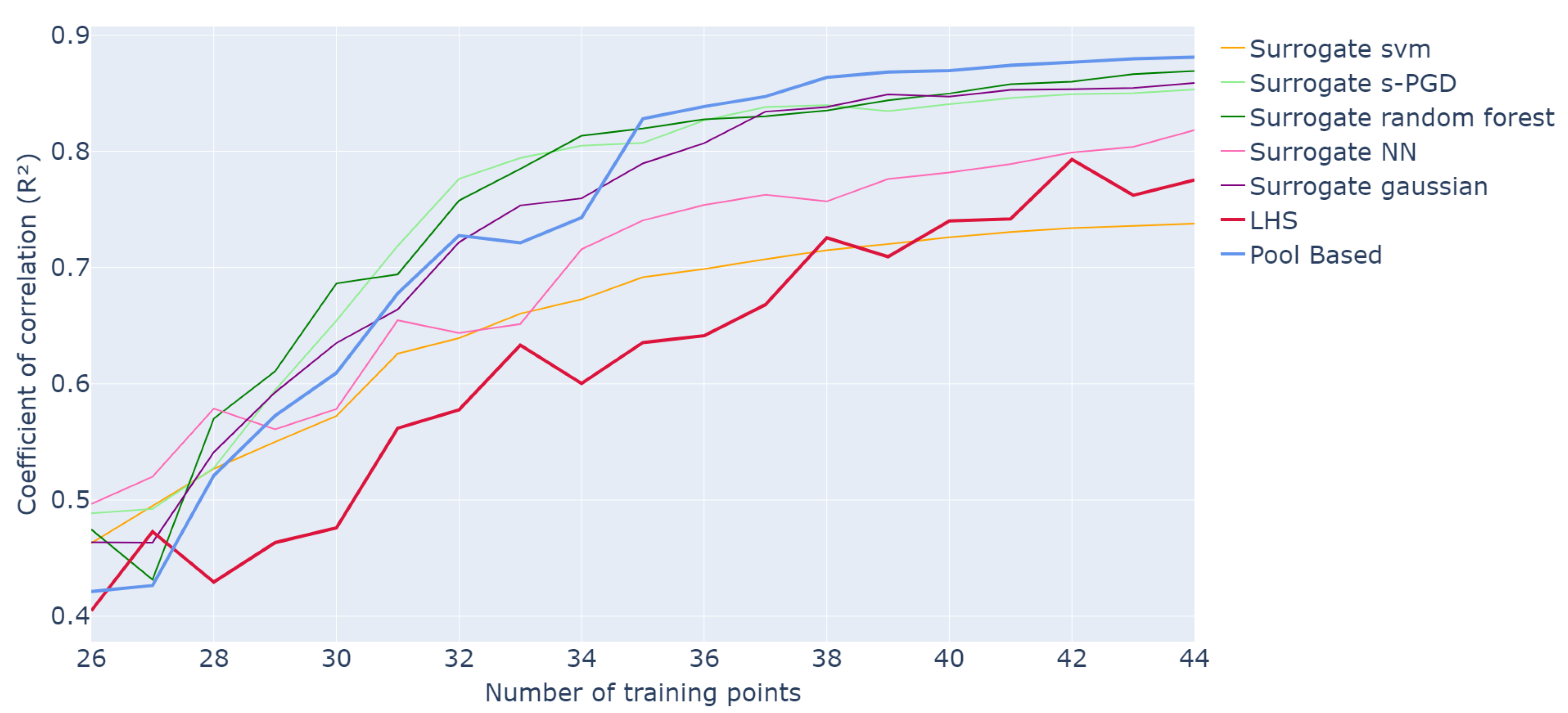
As in the previous approach, the methodology is tested on the 5-dimensional function from Equation (5). The same framework is maintained for training the s-PGD models and comparing the results with LHS and pool-based approaches. Specifically, the pool consists of a ${20}^5$ grid, the initial training sets are LHS samples of size 25, the process is stopped after 20 queries, the $R^2$ values are calculated on the grid test set, and all curves are averaged over 50 iterations of the entire active learning process. Different regression models, including SVR, Neural Networks, Gaussian processes, Random Forests, and s-PGD, were tested as surrogates for the criterion function. These models were implemented using the Scikit-learn library for Python. For each model, the hyperparameters were manually tuned to achieve good $R^2$ values. An LHS of 5000 samples was used to train the surrogate model, a size chosen to balance computational cost and model accuracy. Since this training set is much smaller than the full candidate pool of ${20}^5$ points, the surrogate can be evaluated more efficiently. The best results for each model are plotted thereafter in Figure 6.

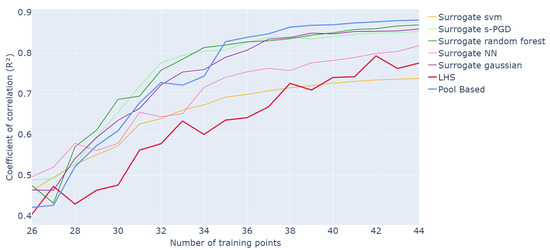
Figure 6. Evolution of R² values for different surrogates of the criterion as a function of the number of points in the training set over 20 runs of the whole active learning process.

The corresponding representative times in seconds are also presented in Figure 7.

Figure 7. Barplot of the representative computing time in seconds for each method.

Here, it appears that the models yielding the best performance are Gaussian processes, Random Forest, and s-PGD. Indeed, the three curves are similar to, or slightly above, the pool-based results. For instance, after 33 queries, they reach $R^2$ values of $0.75$, $0.78$, and $0.79$, respectively, compared to $0.72$ for the pool-based method and $0.63$ for classic sampling.

Regarding computing time, shown in Figure 7, Random Forest and s-PGD appear to be the fastest, taking $38.317$ and $28.308$ s to complete one active iteration, whereas the pool-based methods require $355.3$ s. Gaussian processes also provide substantial time savings, with $139.88$ s versus $355.3$.

Overall, the surrogate method seems to be the most effective as it combines both accuracy and speed.

3.1.6. Global Comparison

Finally, the best results obtained for each methodology are plotted together in Figure 8 and Figure 9 to conduct a global comparison.

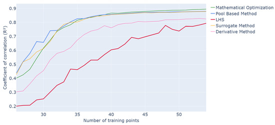
Figure 8. Evolution of R² values for different optimization methods as a function of the number of points in the training set over 20 runs of the whole active learning process.

Figure 9. Histogram of the representative computing time in seconds for each method.

In terms of performance, the mathematical optimization and surrogate method deliver the best performance compared to pool-based sampling, while the derivative method produces slightly less optimal results, consistently outperforming classic LHS. In terms of runtime, the surrogate model and derivative method are the fastest, averaging $28.308$ s and $40.813$ s, respectively, against $355.3$ s for pool-based sampling. Thus, the surrogate method may offer the best balance for achieving both efficient and effective results.

3.2. The 15DResults

These scenario optimizations are especially relevant for high-dimensional problems where defining a refined grid as pool would not be possible or too heavy.

As a second example, and to confirm the generalization of our findings, we aim to estimate the following function in a 15-dimensional input space. This example was chosen to increase dimensionality while keeping the problem within ranges relevant to industrial applications. Moreover, the problem is further complicated by the fact that the function is now composed of sine and cosine terms rather than being purely polynomial.

$$\begin{array}{cc}\hfill f(x& =(x_1,x_2,\dots ,x_{15}))\hfill \\ \hfill & =2cos{x}_1+4sin{x}_2+8sin{x}_3-3sin{x_4}^2+10cos{x_5}^3-2cos{x}_6+sin{x}_7-3sin{x}_8+cos{x_9}^2\hfill \\ \hfill & +2sin{x}_{10}+5sin{x_{11}}^3+3cos{x_{12}}^3-cos{x}_{13}+3cos{x}_{14}-3sin{x}_{15}.\hfill \end{array}$$

(7)

The function is defined on the domain $\Omega ={[-0.5,0.5]}^5$, and the predictions are made over this space using an s-PGD model trained with our active learning criterion. For the training of the model, the s-PGD hyperparameters (modes and degrees) are still set to avoid overfitting and have a good generalization by ensuring an $R^2$ on the training over $0.85$. These values remain fixed along the process. The initial training of the model is an LHS of 25 samples. The process is terminated after 20 queries once convergence of the active learning procedure is achieved and the computational cost is not too high. The training for the surrogate is an LHS of size 20,000. A refined research grid of size $4^{15}$ is used as pool.

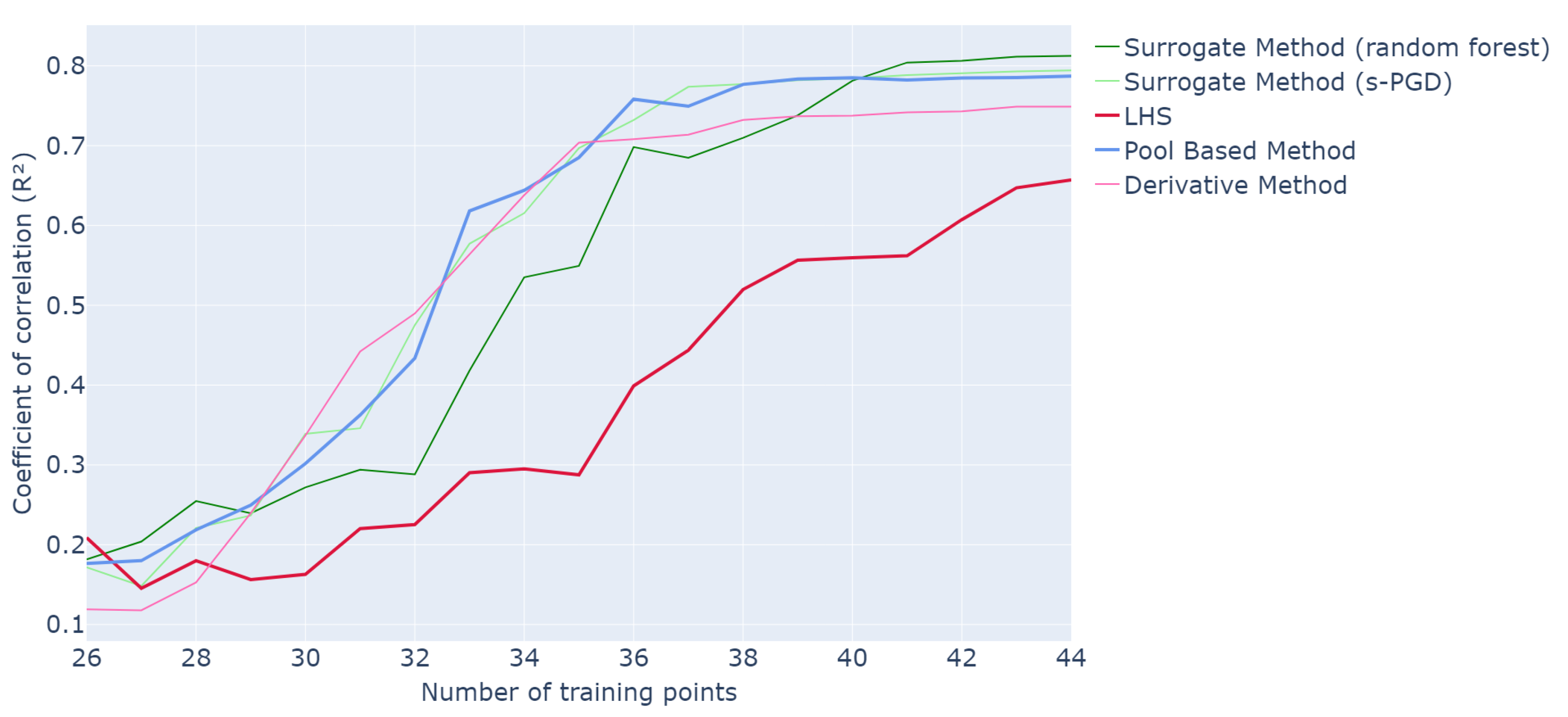
The most efficient methods identified in the 5-dimensional study, namely the surrogate methods using Random Forest or s-PGD, and the derivative method, are selected and tested on this higher-dimensional problem.

The results are presented in Figure 10 for performance and Figure 11 for computational cost.

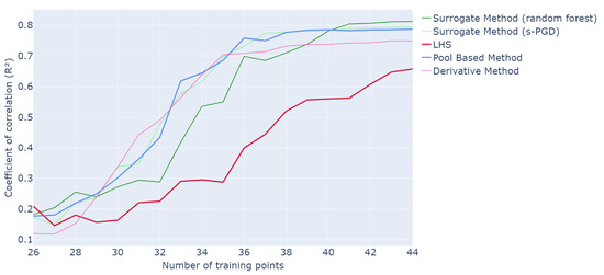
Figure 10. Evolution of R² values for different optimization methods as a function of the number of points in the training set over 20 runs of the whole active learning process.

Figure 11. Histogram of the representative computing time in seconds for each method.

The use of the surrogate method also delivers strong overall performance while providing significant time savings. The results achieved are comparable to those obtained with a pool-based approach, reaching an $R^2$ value of $0.8$ after approximately 40 queries, and are consistently much better than classic LHS. In addition, s-PGD slightly outperforms Random Forest in high dimensions. The computing time for the surrogate methods is slightly lower than that of the pool-based approach. A trade-off can be achieved by using fewer training samples for the surrogate method, which reduces computing time at the cost of some performance; this choice should be guided by the specific requirements of the application.

The results remain encouraging, indicating that good performance can be achieved in high-dimensional settings with relatively few samples. Although the computational cost of evaluating a single output in this example is modest, the potential efficiency gains would be even more significant in real industrial applications, where each evaluation is more expensive.

It is also worth noting that the derivative method achieves performance close to the pool-based approach, although slightly lower. However, its computing time is considerably higher, making it unsuitable for high-dimensional problems. Therefore, the surrogate method emerges as the preferred choice.

4. Initialization Study

On the other hand, although much effort has been spent on designing new active learning algorithms, little attention has been paid to the initialization of active learning.

4.1. Literature Review

4.1.1. Actively Initialize Active Learning

There are few studies on how to initialize the active learning process. Some ideas, such as clustering-based approaches (k-means), inspired methodologies, or optimal design-based approaches, are proposed to actively initialize active learning in [14]. However, to date, the performance of these approaches has been demonstrated solely for classification problems. Most articles already assume the existence of the initial set in their studies.

4.1.2. Design of Experiments

The first idea that comes to mind is to use a classic DOE, such as Full Design [21], Factorial Design [22], or Plackett–Burman [24], to start the process. Unfortunately, designs such as Full Design or Factorial Design have too many samples, and others, such as Plackett–Burman, are too small. In general, the number of samples is not adaptable and depends on the dimension of the problem, which is a main constraint.

4.1.3. Space-Filling Design

However, within the DOE field, a sub-field called space-filling design [37] has interesting properties. Indeed, space-filling designs ensure that the sampling covers the entire design space in a balanced and representative manner. This uniformity helps in reducing bias and ensures that no particular region of the design space is under-represented.

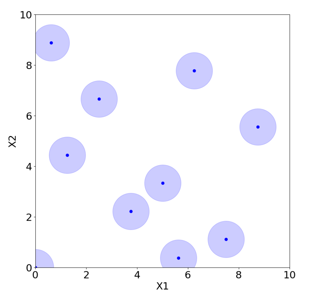
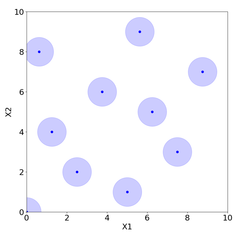
LHS, for instance, belongs to space-filling designs. To construct a Latin hypercube of n samples, the range of each of the factors is divided into n equally spaced intervals. Then, one coordinate of a design point is sampled from each of the intervals. In this way, there is only one point in each row and column. Therefore, if we are conducting an experiment with multiple factors but are only interested in one because the other factors do not influence the output, all the different experimental conditions will only show the influence of the one factor we are focusing on. As a consequence, we will see outputs associated with just the different levels of that one factor without any interaction effects from the other factors. The design points will thus be aligned with the distinct levels of this single factor, making it the only source of variation in the experiment.

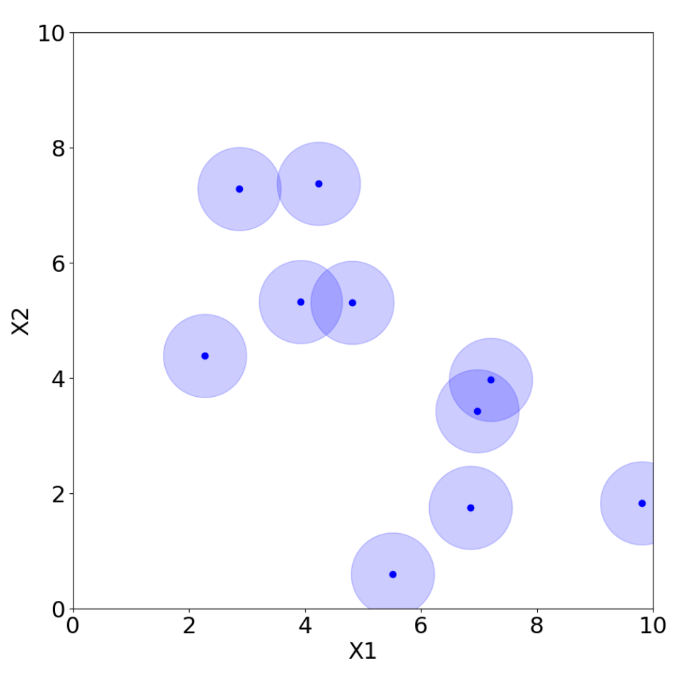
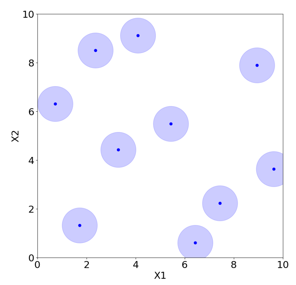
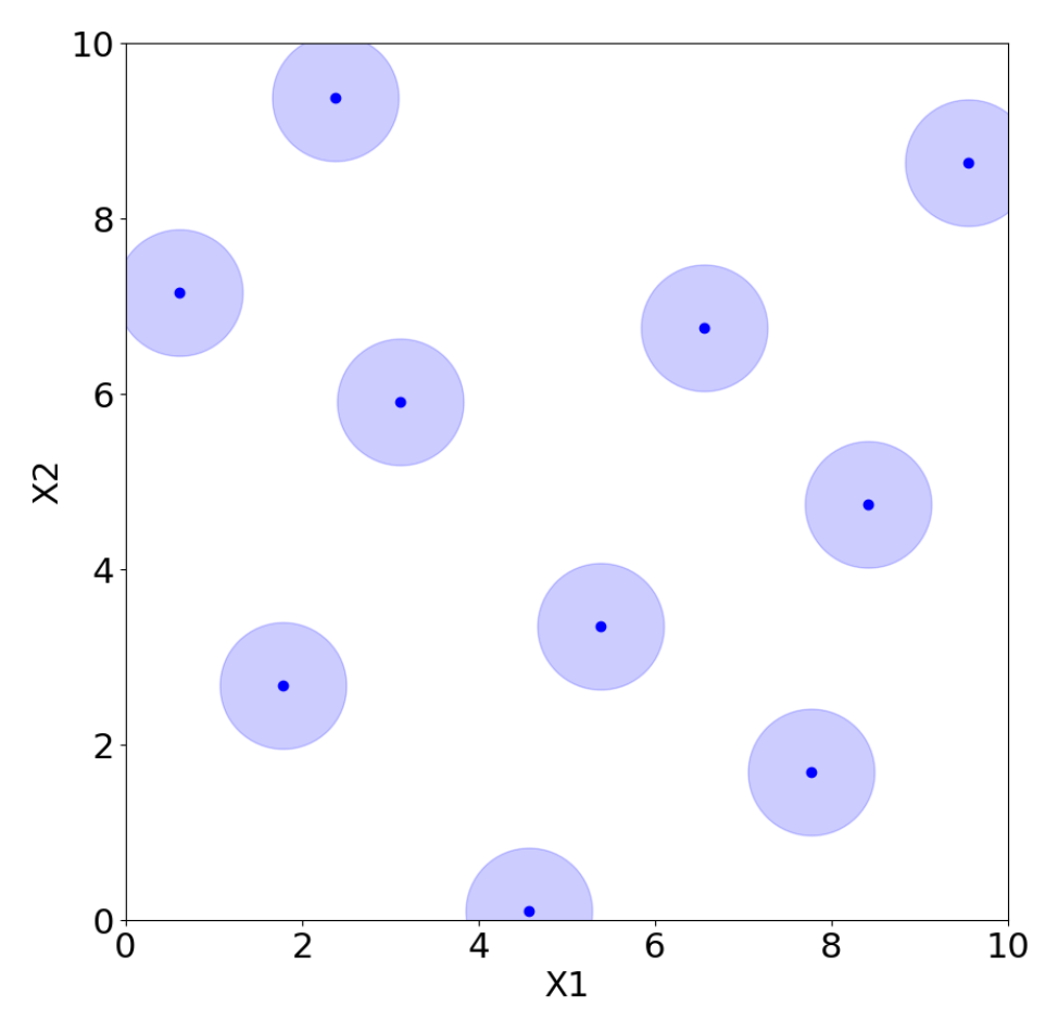
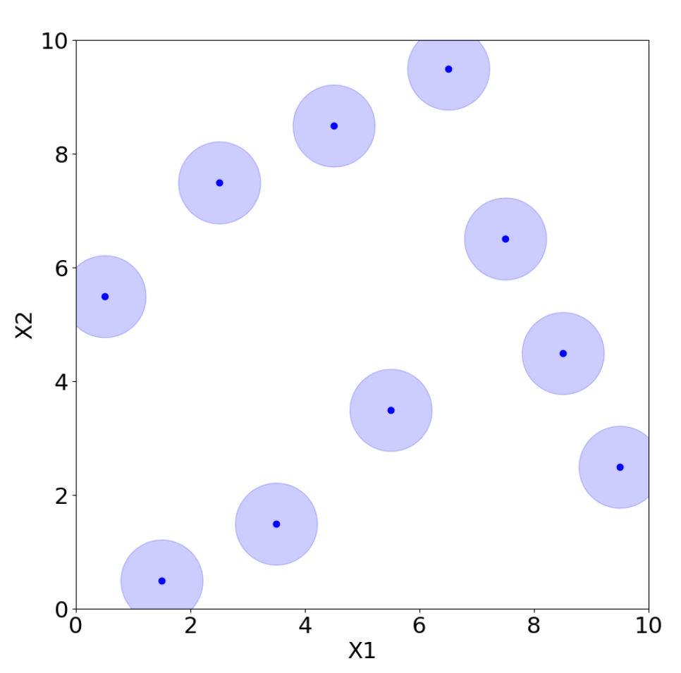
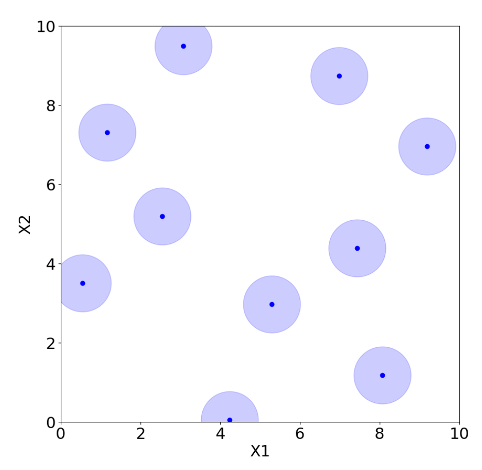
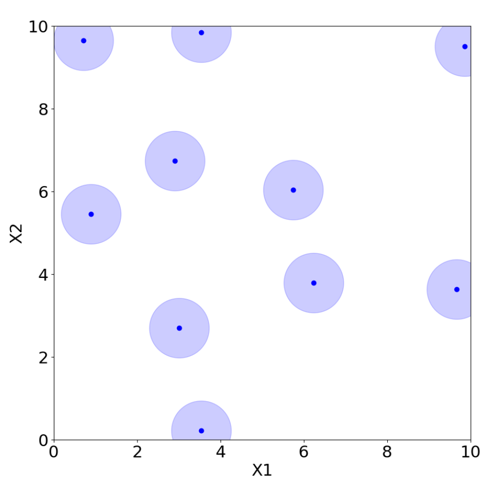
However, there are many possible choices for LHS, and not all of them are adequate. For example, placing the points on the diagonal produces an LHS, but it is clearly a poor design choice. Morris and Mitchell [38] propose, for example, maximin Latin hypercube sampling (MmLHS), which maximizes the minimum distance among the points. Many other variations of the criterion exist, such as centered LHS (optimized LHS with points set uniformly in each interval) [23], correlation LHS (optimized LHS by minimizing the correlation) [39], and ratio LHS (optimized LHS by minimizing the ratio ${\displaystyle \frac{max\left(pdist\right)}{min\left(pdist\right)}}$) [40]. All these methods are illustrated in Figure 12, Figure 13, Figure 14, Figure 15, Figure 16 and Figure 17 for two parameters, $x_1$ and $x_2$, where each point represents a sample from the corresponding design with coordinates $(x_1,x_2)$. The light blue area around the points is added only to improve their visibility and highlight their locations.

Figure 12. Random sampling.

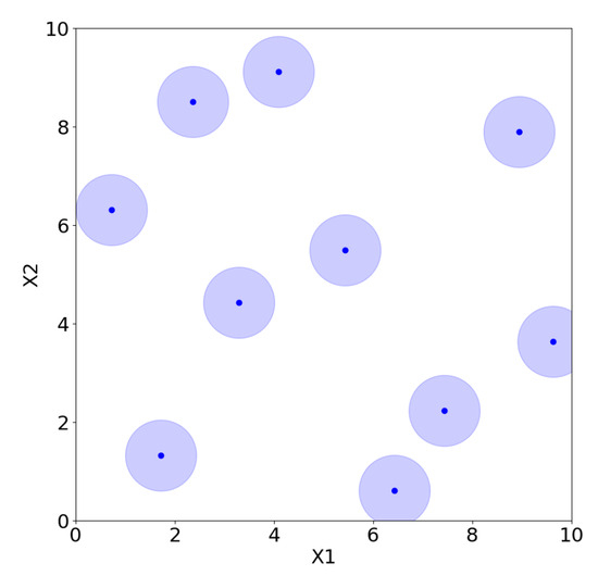
Figure 13. Classic LHS.

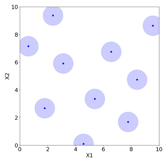
Figure 14. MmLHD.

Figure 15. Centered LHS.

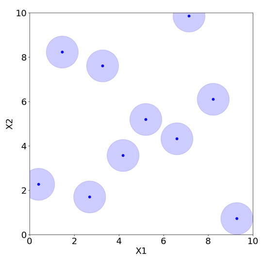
Figure 16. Correlation LHS.

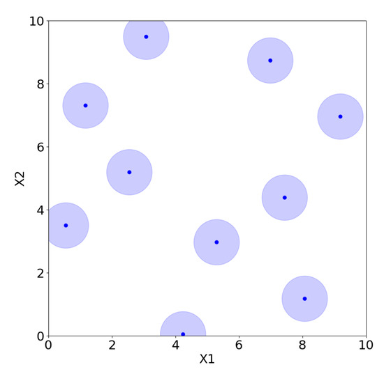
Figure 17. Ratio LHS.

In general, and as illustrated in Figure 12, Figure 13, Figure 14, Figure 15, Figure 16 and Figure 17, LHS designs lead to a well-distributed coverage of the input space, ensuring that samples are spread across all dimensions and that the entire domain is explored uniformly.

Other usual space-filling designs are minimax and maximin distance designs [41]. Minimax and maximin distance designs are approaches used to optimize the arrangement of experimental runs to minimize or maximize a certain criterion related to distances between samples.

Minimax distance designs’ goal is to minimize the maximum distance between any two points in the design space (various metrics, such as Euclidean distance or some other measure, can be used to quantify the dissimilarity between samples). By minimizing the maximum distance, the design aims to be robust against potential variations, ensuring that the estimated effects of factors are not overly sensitive to change.

Maximin distance designs seek to maximize the minimum distance between any two points in the design space. In other words, the goal is to ensure that, even under the worst-case scenario, there is a maximum amount of space between experimental runs. These designs are useful when the samples need to be as spread out as possible over the input space. This is especially relevant in situations where resources are limited and it is crucial to make the most out of the available resources.

As presented in Figure 18 and Figure 19, the maximin design produces evenly spaced samples across the domain, while the minimax design ensures that no region of the space appears uncovered.

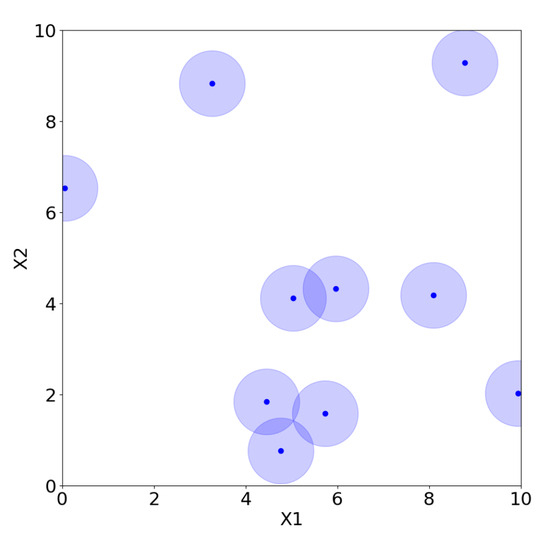
Figure 18. Maximin distance design.

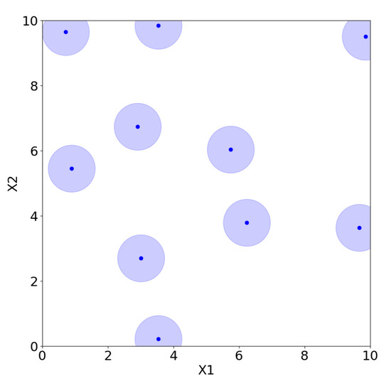
Figure 19. Minimax distance design.

Finally, a sequence-based approach can be considered. Indeed, Halton and Hammersley sequences are deterministic sequences that are often used in the construction of experimental designs [42], especially in the context of quasi-Monte Carlo [43] methods and low-discrepancy sampling [44]. These sequences enable systematic generation of points in a multidimensional space that exhibit low discrepancy, that is, a more even distribution compared to purely random sequences.

Halton sequences are constructed using coprime bases for each dimension [45]. The process involves three steps: representing integers in the chosen basis, reversing their digits, and then mapping the reversed representation to a fractional number within the interval [0, 1]. This process is repeated for each dimension with a different prime basis, ensuring low discrepancy and uniform coverage. The Hammersley sequence [46] is a special case of the Halton sequence. It is built by fixing one dimension and using Halton sequences for the other dimensions. This approach enhances uniformity in the point distribution.

Sobol sequences [47] are also quasi-random sequences used to obtain a uniform sampling across multidimensional spaces. They are constructed using a deterministic algorithm based on binary arithmetic. Visually, this leads, as plotted in Figure 20, Figure 21 and Figure 22, to a uniform and well-dispersed coverage of the input space.

Figure 20. Halton.

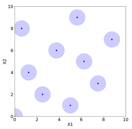
Figure 21. Hammersley.

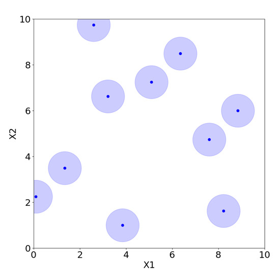
Figure 22. Sobol.

To initiate an active learning process, space-filling designs might be beneficial due to their capacity to homogeneously fill the space.

4.2. The 5D Results

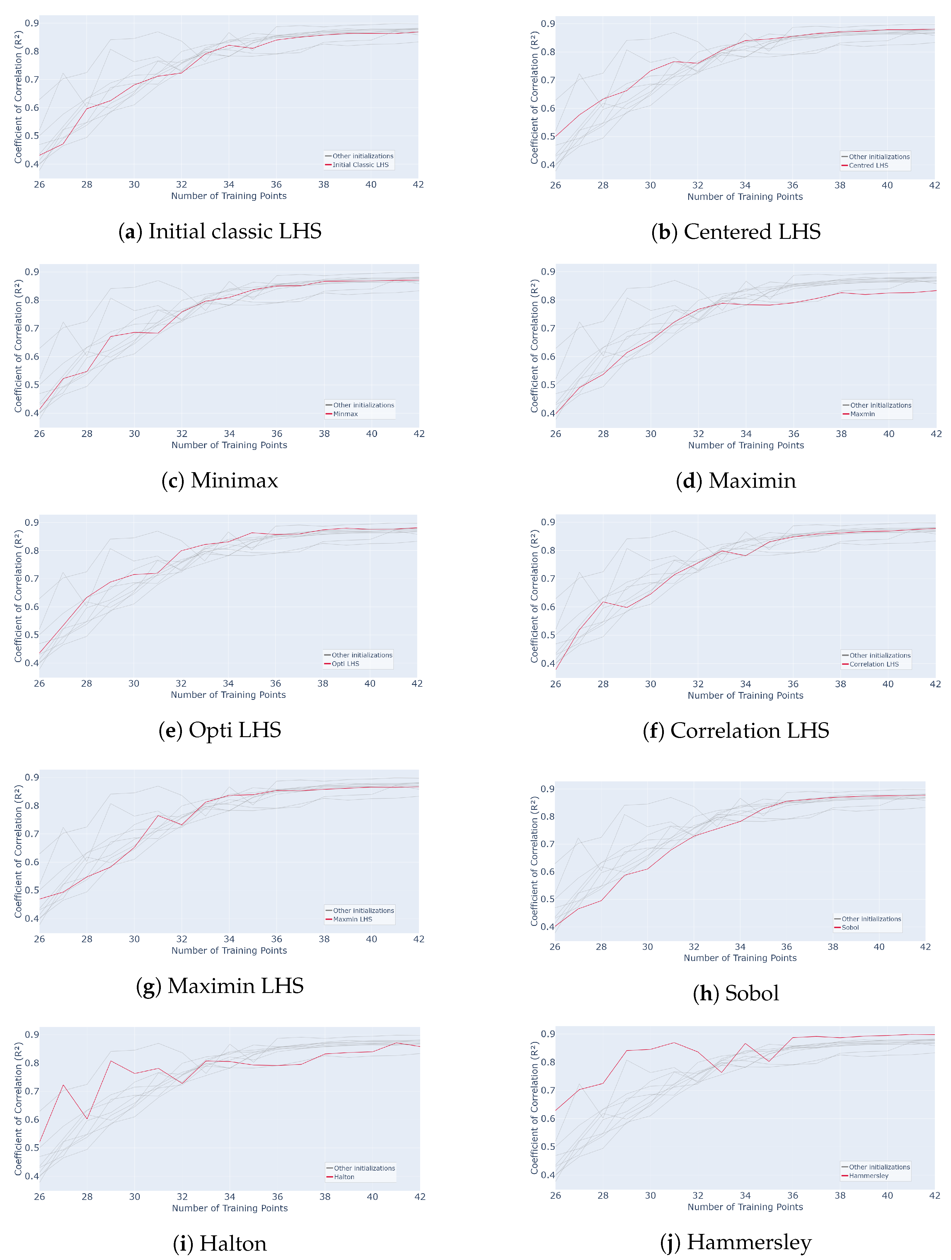
The different methodologies described in this study are tested as an initialization for our active learning criterion. The scenario used is a pool-based sampling on a ${20}^5$ grid, and the function is the five-dimensional problem of Equation (5). The initial training set consists of 25 samples, and the process is terminated after 17 queries upon reaching convergence. The s-PGD regressor is set as before to reach an $R^2$ above $0.85$ on the training. The test set is the remaining samples of the pool.

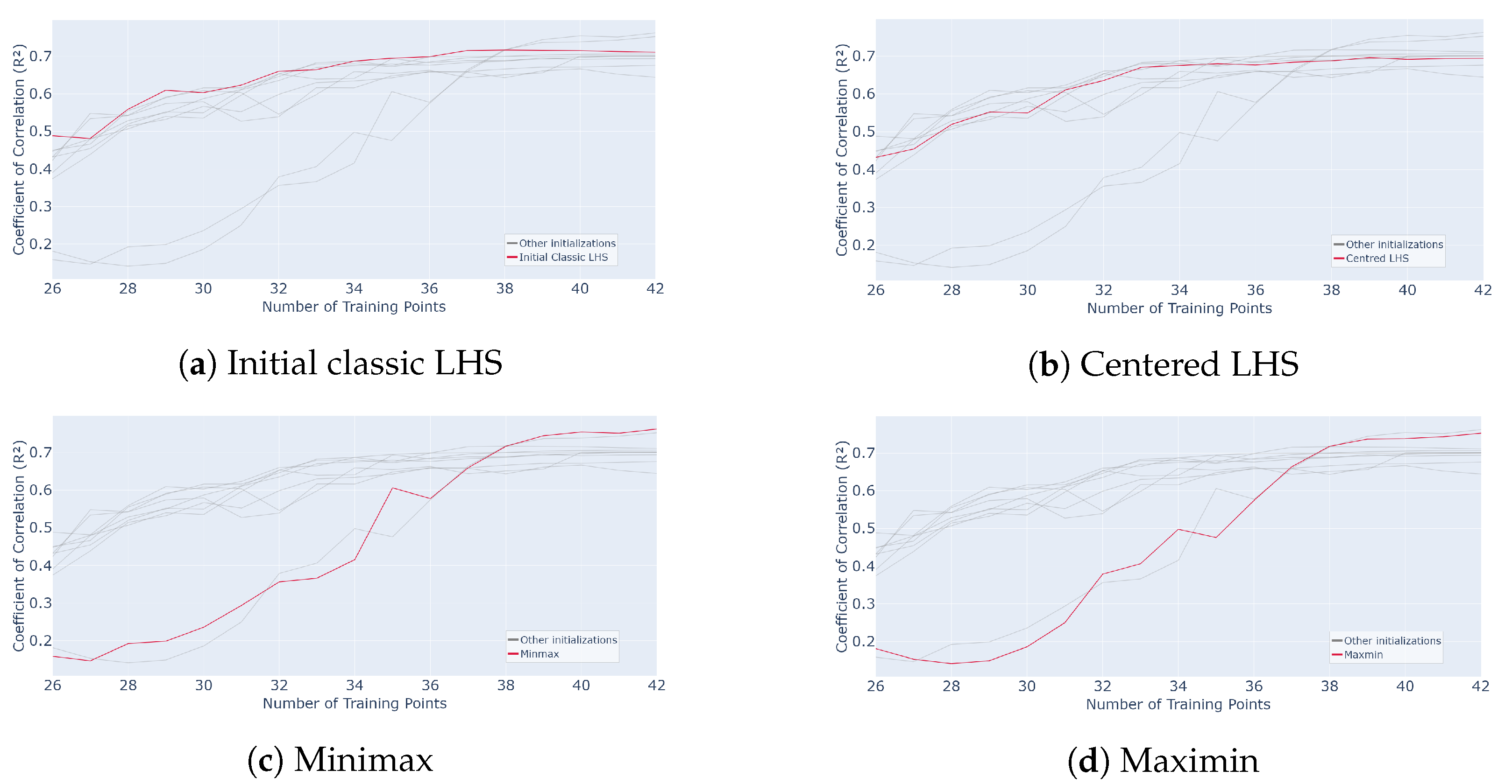
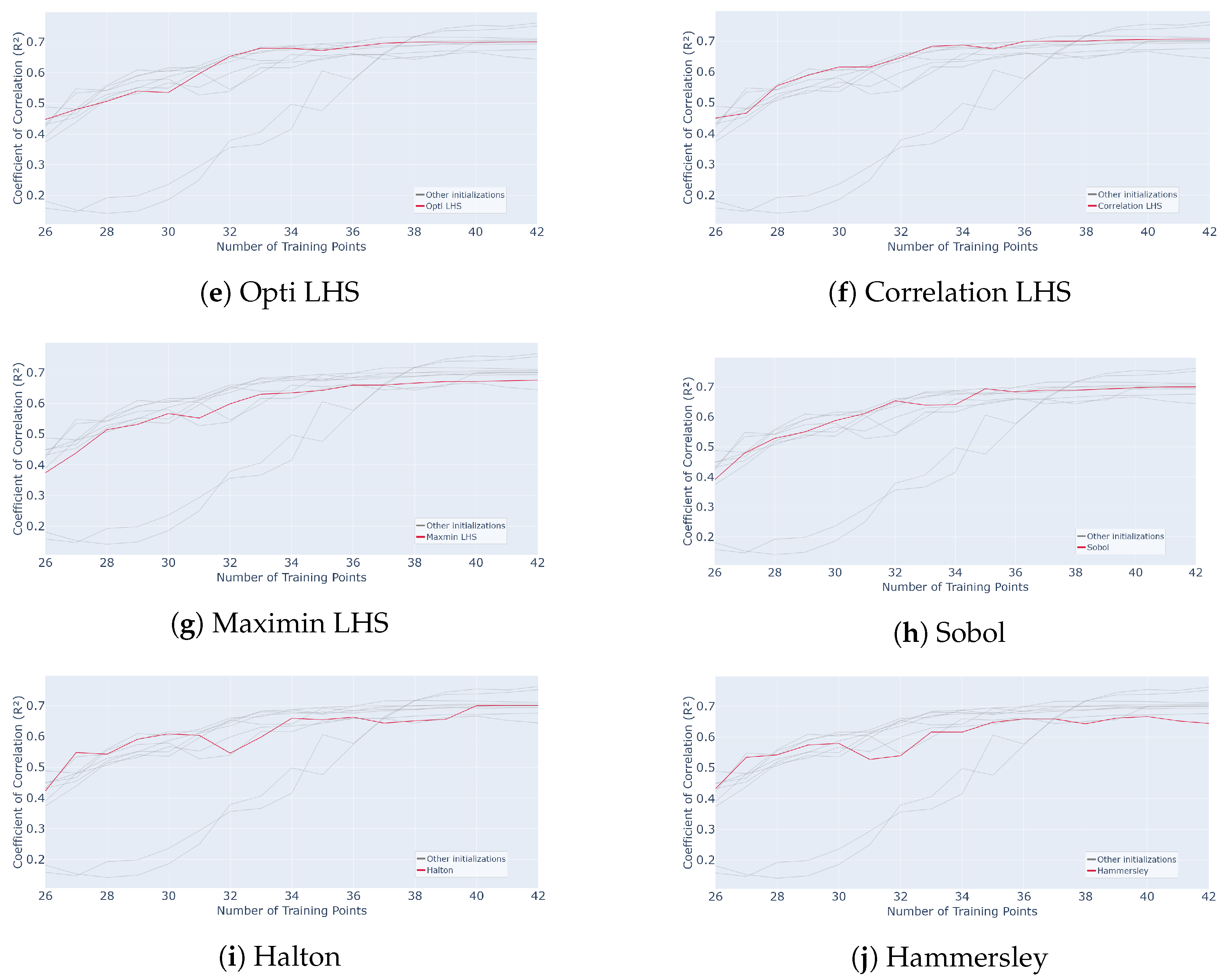
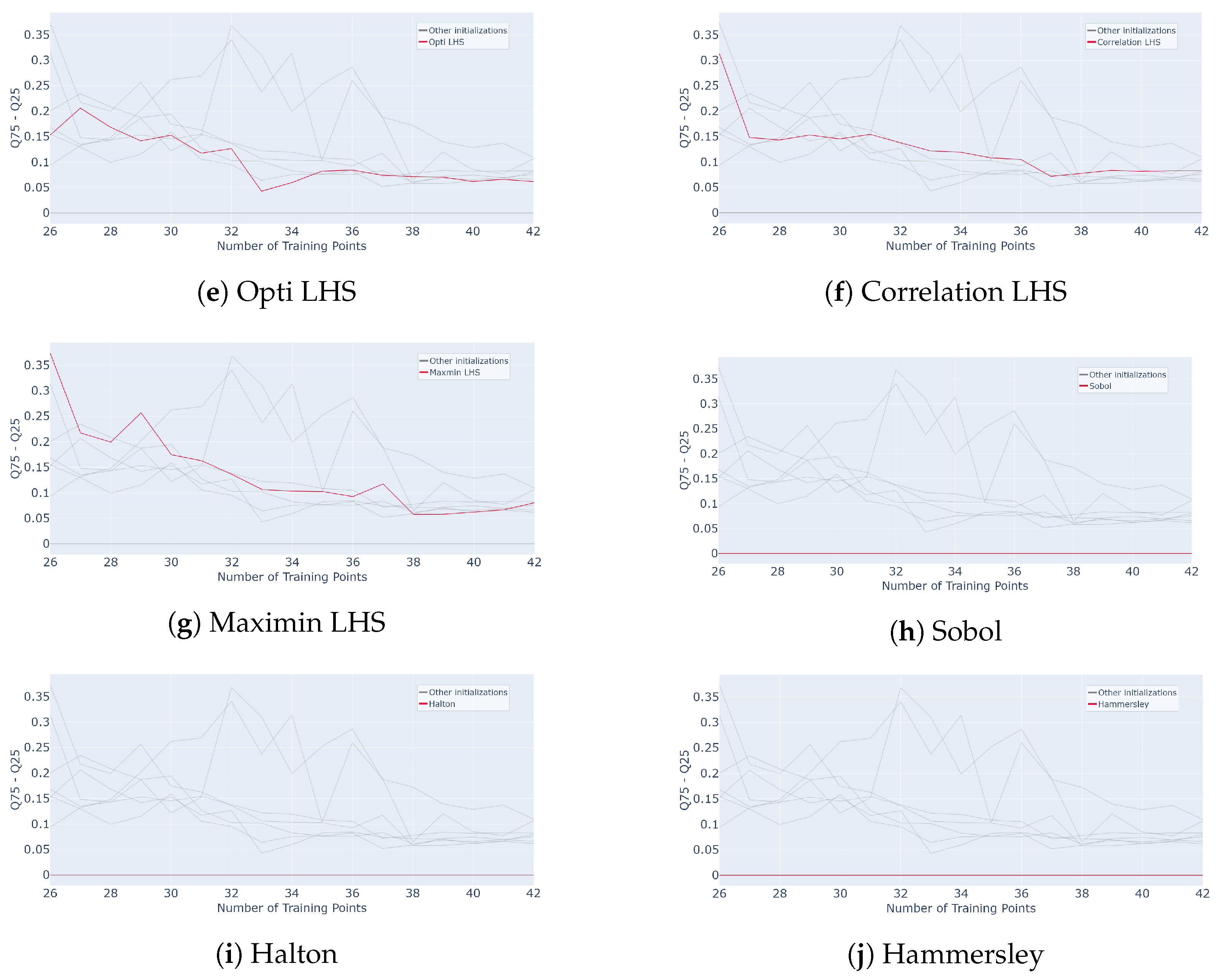
The average $R^2$ value on the remaining samples of the grid and over 50 repetitions of the whole process is calculated. The results are shown in Figure 23. The red curve represents a process initialized with 25 samples using the method indicated in the legend, while the gray curves correspond to the other initializations tested for comparison.

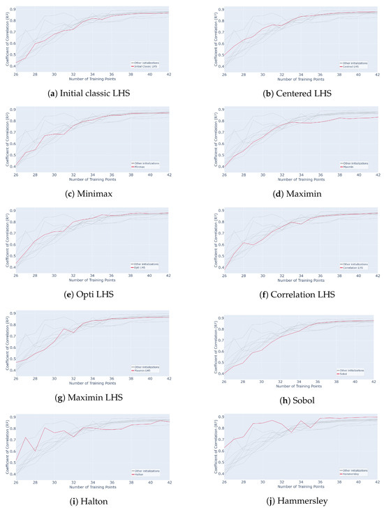
Figure 23. Evolution of $R^2$ for different initialization designs mentioned in subcaption (Classic LHS, Centred LHS, Minimax, Maximin, OptiLHS, Correlation LHS, Maximin LHS, Sobol, Halton and Hammersley) as a function of the number of points in the training set over 50 runs of the whole active learning process.

It appears that the initializations yielding the best average results in the active process are the Hammersley and Halton methods. Indeed, their performance curves are above the others throughout the process, especially at the beginning. The Hammersley and Halton methods reach, for example, $0.82$ and $0.84$, respectively, as $R^2$ values for 32 samples. However, all the methods perform well on average. Indeed, adding samples increasingly yields an average correlation value around $0.76$ for 32 samples for any initialization, while it only reaches $0.55$ with an LHS in [15].

In this study, the point of interest is the variability and impact of the initialization on the active learning process. Indeed, as observed in [15], an active process initialized with a classic LHS yielded sufficient results on average, but the interquartile range was, initially (after 1 query), around $0.20$, meaning the dispersion was notable. It then decreased quickly, reaching $0.05$ around 10 queries. The LHS seeks to increase the inertia by starting in random directions, which explains this dispersion phenomenon. This led to variability in the performance of the whole active process.

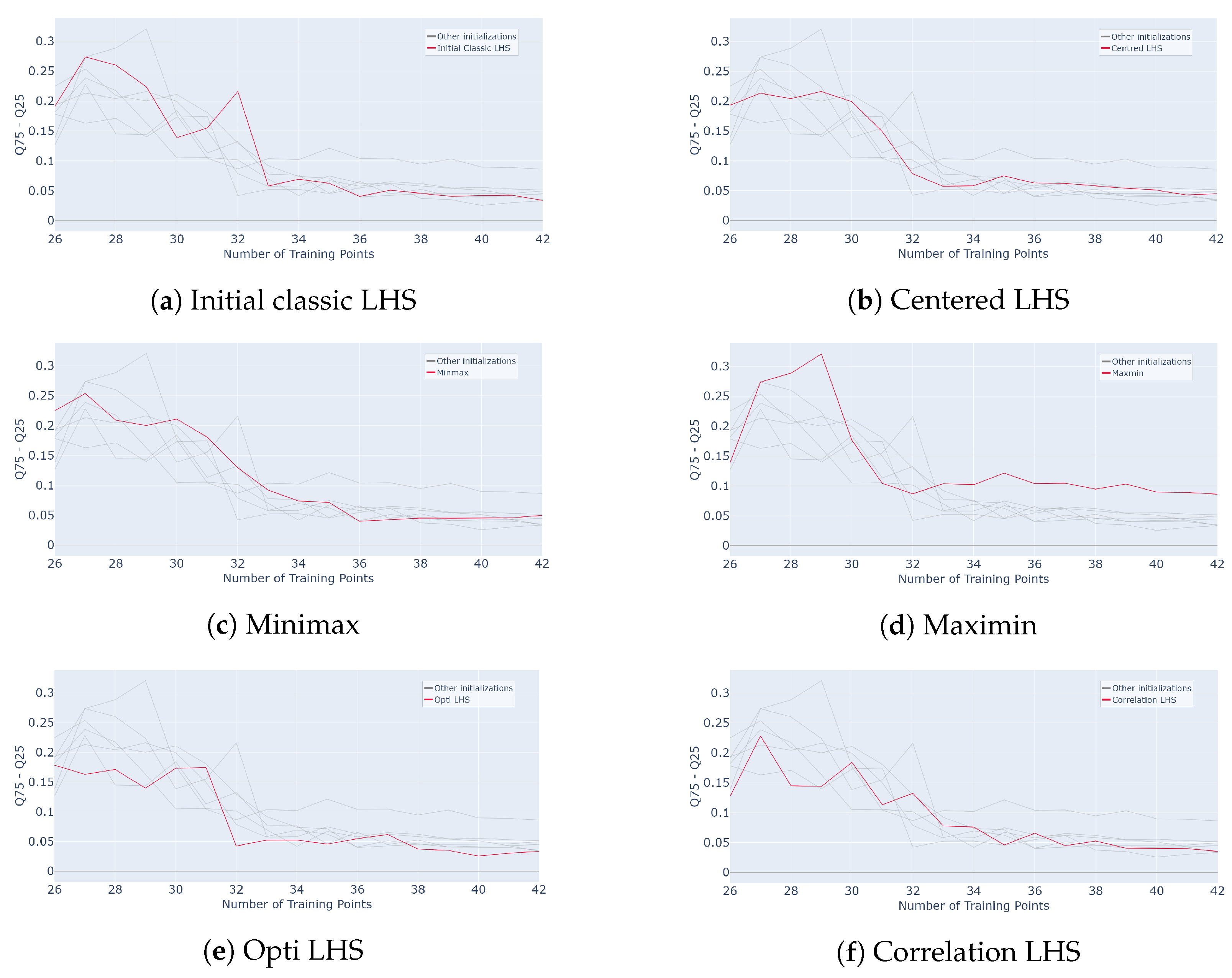
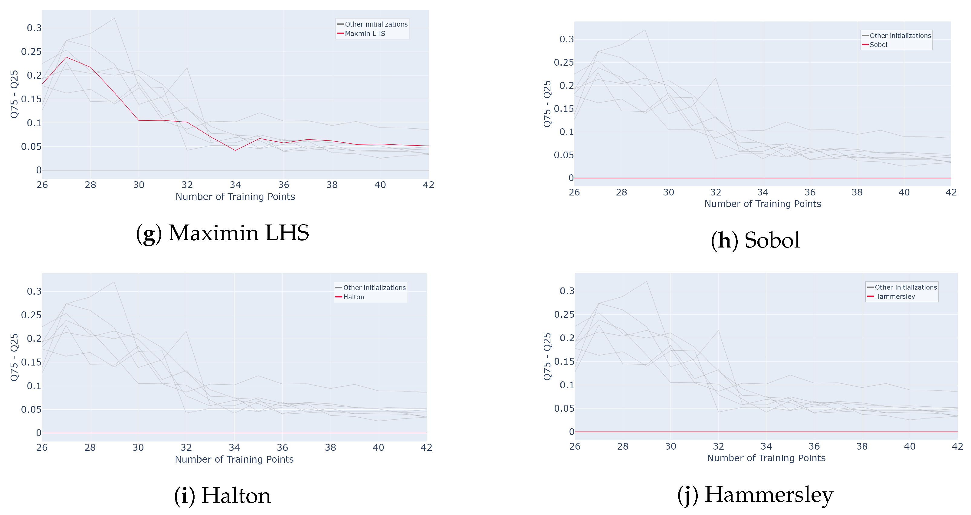
To highlight the impact of initialization on subsequent results, the interquartile range of $R^2$ was calculated for each method and iteration and is plotted in Figure 24. This interquartile range is defined as the absolute value of the difference between the last and first quartile of $R^2$ at one considered step of the active process.

$$EI=\mid R_{Q3}^2-R_{Q1}^2\mid$$

(8)

where $R_{Q3}^2$ and $R_{Q1}^2$ are, respectively, the last and first quartiles of the $R^2$ values at the considered iteration. The averaged results are plotted in Figure 24. The red curve is the initialization method considered in the legend, and the gray curves are all the others for comparison purposes.

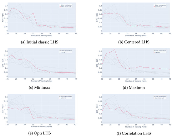
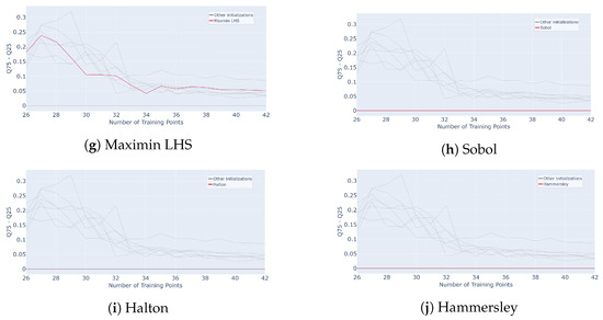
Figure 24. Evolution of interquartile range for different initialization designs mentioned in subcaption (Classic LHS, Centred LHS, Minimax, Maximin, OptiLHS, Correlation LHS, Maximin LHS, Sobol, Halton and Hammersley) as a function of the number of points in the training set over 50 runs of the whole active learning process.

As expected, the Hammersley and Halton methods do not show variability. In fact, these samplings are built from sequences and remain the same for fixed parameters. The various LHS methods, on the other hand, exhibit more variability, especially at the beginning, starting around $0.2$, and then the $R^2$ decreases and reaches a plateau value around $0.05$. As noted in the previous section, this type of sampling is built iteratively from a random selection, which leads to different possible outputs. The same holds for the minimax and maximin samplings.

To obtain more reliable results, the Halton and Hammersley sequences prove to be the most efficient initial settings. These initial samplings ensure strong overall performance of the active learning process. It remains to be verified, however, whether this finding also holds in higher-dimensional settings.

4.3. The 15D Results

The same tests are performed on the 15-dimensional function from Equation (7). We consider our active criterion and a pool-based scenario with a $4^{15}$ grid. The $R^2$ values calculated on the remaining samples of the pool are extracted for each iteration and averaged over 50 repetitions of the whole process. The initial training set consists of 25 samples, and the process is terminated after 17 queries upon reaching convergence. The s-PGD regressor is tuned as before to reach an $R^2$ above $0.85$, and these hyperparameters remain unchanged along the process. The test set is the remaining samples of the pool. The results are plotted in Figure 25. Each red curve corresponds to a process run with the initialization indicated in the legend. The gray curves are all the other initializations for comparison purposes.

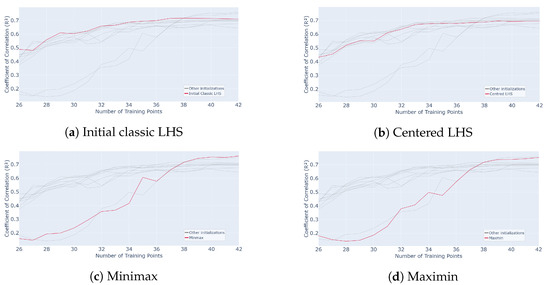
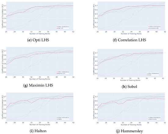
Figure 25. Evolution of $R^2$ for different initialization designs mentioned in subcaption (Classic LHS, Centred LHS, Minimax, Maximin, OptiLHS, Correlation LHS, Maximin LHS, Sobol, Halton and Hammersley) as a function of the number of points in the training set over 50 runs of the whole active learning process.

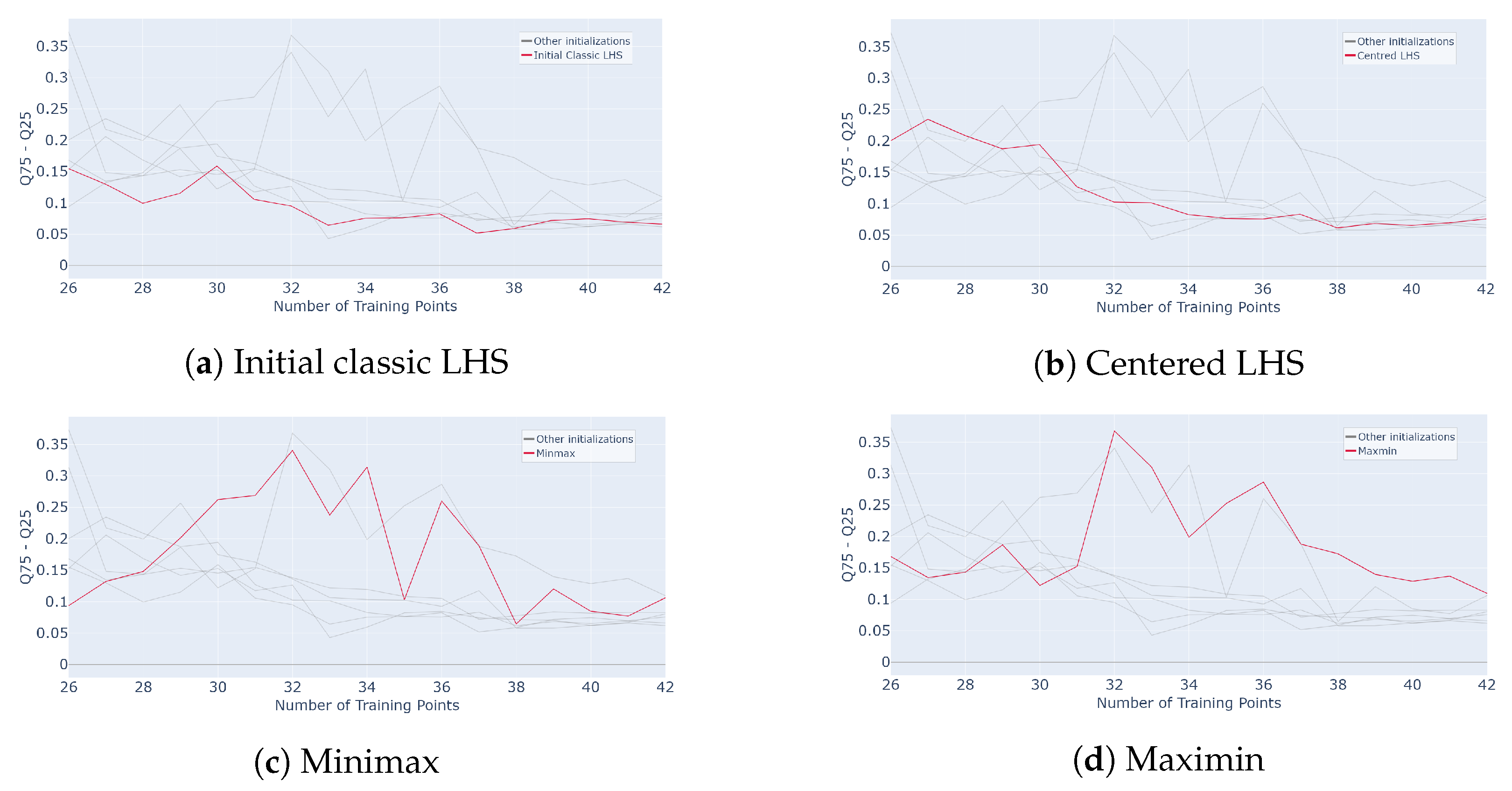
Then, the interquartile ranges are calculated and plotted in Figure 26.

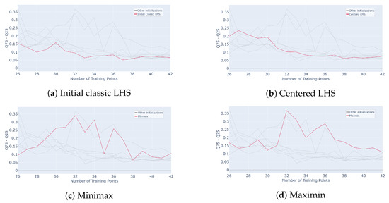
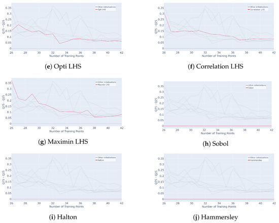
Figure 26. Evolution of interquartile range for different initialization designs mentioned in subcaption (Classic LHS, Centred LHS, Minimax, Maximin, OptiLHS, Correlation LHS, Maximin LHS, Sobol, Halton and Hammersley) as a function of the number of points in the training set over 50 runs of the whole active learning process.

In terms of performance, LHS and sequential designs exhibit a similar pattern, with a noticeable improvement during the first sample additions followed by a plateau. LHS sampling achieves high convergence but shows significant variability, ranging from $0.2$ to $0.05$, making it less reliable for very few queries. Maximin and minimax initializations display slower initial growth, with a gradual increase in performance for the first few queries, but they eventually converge to higher final values, $0.75$ and $0.76$, after 17 queries. However, they maintain high variability throughout, reaching $0.35$ after 7 queries, which makes them more uncertain in early stages. In contrast, Halton and Hammersley sequences provide slightly lower convergence, $0.748$ and $0.741$, respectively, after 17 queries, but their early-stage performance is strong, starting higher at $0.43$ for a single query, and their variability is null, making them highly robust. Compared to Figure 10, where an $R^2$ of $0.4$ is reached with 36 samples for a classic sampling, all these methods converge faster here, reaching around $0.67$.

Overall, using Hammersley and Halton sampling to initialize s-PGD active learning produces robust and reliable performance, even in high-dimensional settings. While their final performance may be slightly lower than other methods, their deterministic nature ensures consistent and repeatable results, making them particularly well suited for industrial applications involving complex and costly problems.

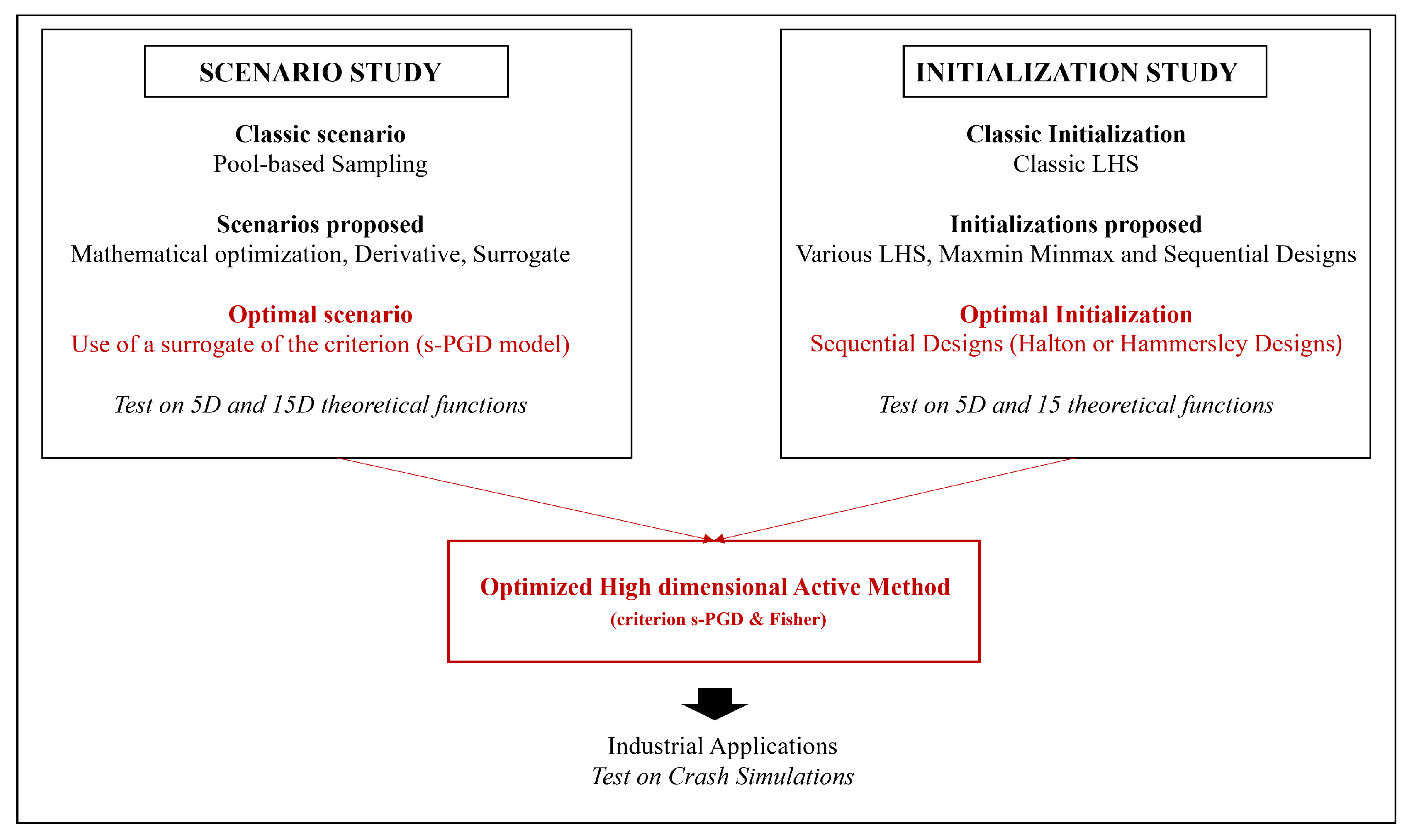
To summarize the results from Section 3 and Section 4, the optimal global methodology from our study is the use of a surrogate model (s-PGD) for the scenario and an initialization test based on a Halton or Hammersley design. The combination of these two elements provides an efficient active methodological framework for high-dimensional industrial problems, which should be further tested on real applications. A summary of this method is presented in the workflow shown in Figure 27 before industrial testing.

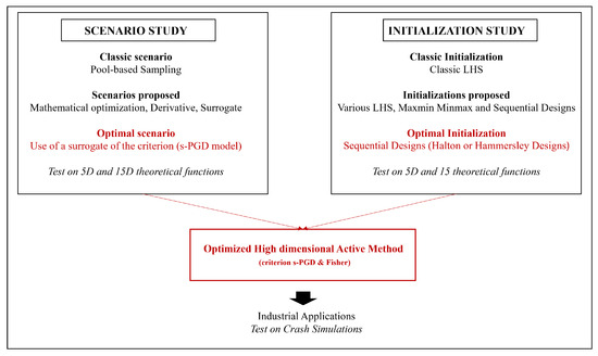
Figure 27. Workflow of the methodology and results developed in the article.

5. Industrial Application

Time efficiency is crucial in industrial applications, where data production is often very costly. Additionally, assessing the certainty of good results is vital because averaging multiple runs of the entire process would be too time-consuming or computationally intensive.

This is why these methods are currently applied to an industrial mechanical problem using a pi-beam deformation example. The goal is to study and predict the deformation of a mechanical structure consisting of nine parts, each with a specific thickness. The model is depicted in Figure 28.

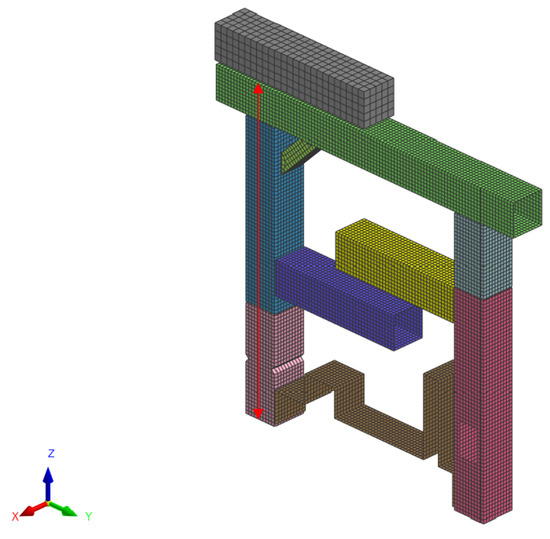
Figure 28. Structure of the pi-beam and settlement of the problem.

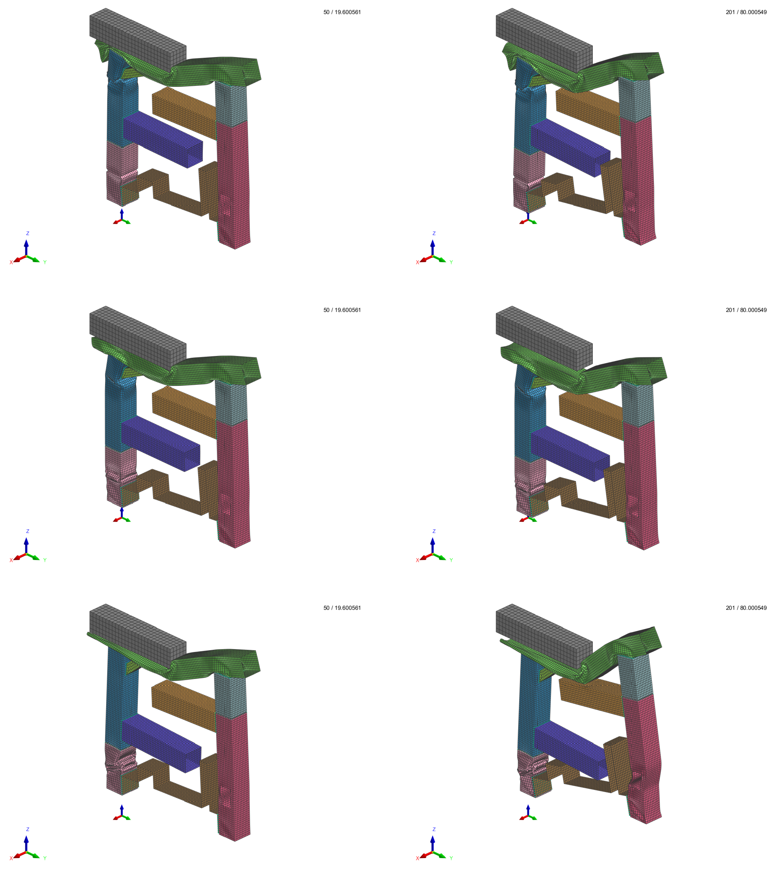
The application of constant stress smashes the beam along the z-axis. The corresponding deformation depends on the thickness chosen for the nine parts. Some cases are represented in Figure 29, where the intermediate and final time steps for different input thickness values are illustrated.

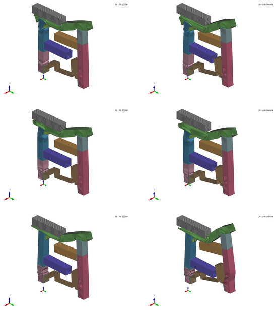
Figure 29. Visualization of pi-beam simulation results at intermediate (left) and final (right) time steps for 3 cases with different input thickness values for the nine parts.

The pi-beam is a classic test for computational mechanics of particular interest in the automotive industry. In this case, the model’s aim is to estimate the intrusion, which is the distance represented with the red arrow in Figure 28. The intrusion stands for the displacement that would occur in the cockpit of a car under crash conditions. The pi-beam is a simplified mechanical representation of the front end of a car, making it a useful benchmark for safety-related studies. In the automotive context, accurately modeling such behavior with surrogate models is particularly valuable as it significantly reduces computational time compared to full-scale finite-element crash simulations. This acceleration not only facilitates design space exploration and optimization of structural components but also enables near real-time evaluations, which are essential for iterative design cycles and virtual prototyping in industrial applications.

In our model, the intrusion is measured at the final simulation time step function of the thicknesses chosen for each box as input parameters $(h_1,h_2,$…$,h_9)$. The range of the thicknesses is 1 to 1.7 mm. The simulations were carried out using the commercial software VPS (version 2022) from ESI Group. ESI Group is considering the proposed technology addressed in the present paper within the AdMoRe ESI solver.

As in the previous sections, we will compare the performance (in terms of $R^2$ values) for s-PGD models trained with our active criterion in a classic pool-based and LHS initialization framework, our criterion combined with the new optimal initialization and scenario, and an LHS with the same number of training samples.

The initialization for the pool-based active method is performed with an LHS of 25 samples. The pool to select the next sample is defined as a research grid of 9 subdivisions along each axis, yielding a pool of $9^9$ elements to be precise enough. Moreover, the whole process is repeated 20 times to produce an average of the results obtained. Due to the balance between performance and cost of the simulations, the process is stopped after 44 training samples.

The test set for all is composed of 1000 samples selected with an LHS to cover the parametric space. The s-PGD hyperparameters have an $R^2$ value on the training above $0.85$, remaining fixed for all. As a result of the studies regarding initialization and numerical optimization of the scenarios, we decided to evaluate on this test case an s-PGD surrogate for the criterion and sequential designs for initialization. Halton and Hammersley are tested.

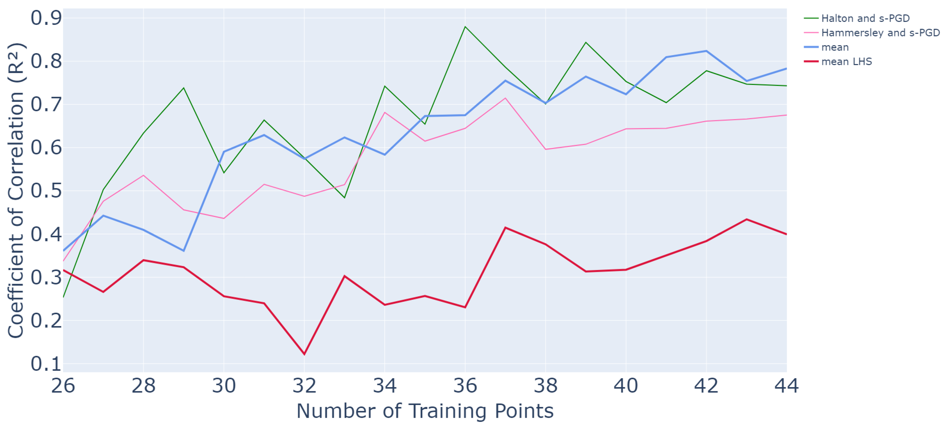
The results are plotted in Figure 30.

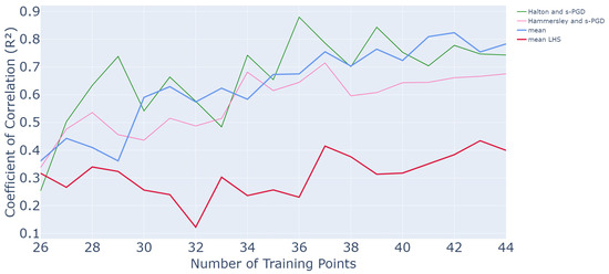
Figure 30. Evolution of $R^2$ values as a function of the number of points in the training set for the pi-beam application.

It appears that both optimized methods with Halton and Hammersley initializations and an s-PGD surrogate yield good results. For the Halton and surrogate method, the performance is quite similar to that obtained with a nonoptimized active method (mean curve). An $R^2$ value of $0.74$ is reached after 8 queries, and the method converges then. For the Hammersley and surrogate method, the performance is slightly below that obtained previously but remains good. Indeed, an $R^2$ value of $0.68$ is reached after 8 queries, and the method converges around this value thereafter. Both still provide much better results than an LHS, which only reaches $0.3$ for 44 training samples.

In terms of time efficiency, both methods yield considerable reductions in runtime. Indeed, for the pi-beam, it takes 48,502 s to perform one whole run of the active learning process without any optimization. With the use of an s-PGD surrogate of the criterion, it takes 46,256 s. Then, with an appropriate initialization, we only need to run the process once, so the global amount of time is 46,256 s, which is around half a day. In comparison, with LHS initialization, the process was repeated 20 times, so it took around 10 days to run. Thus, in this intermediate-cost industrial application, the proposed optimized method achieves substantial time efficiency.

Both improvements combined, initialization and scenarios, give rise to a new optimized active method that is just as efficient and faster. This is particularly relevant for industrial applications where computational cost and running time are main issues. However, this methodology can still be improved and studied regarding some practical points, such as applying it to experimental data, which has not been undertaken yet.

6. Conclusions and Future Works

To sum up, our objective was to study the initialization and scenario design and their impact on the active learning process, as well as to propose an optimal methodology for both in high-dimensional industrial contexts. For this purpose, we used an information criterion specifically tailored to such settings, which combines the Fisher matrix with a Sparse Proper Generalized Decomposition (s-PGD). Based on this framework, we conducted an in-depth study of sampling scenarios and initialization strategies.

On the one hand, the scenarios used in current active learning processes can be highly computationally demanding and time-consuming and therefore require improvement. This is why the classic pool-based scenario was modified using surrogate, derivative, and mathematical optimization approaches. The results show that using a surrogate approach provides the best balance between accuracy and computational efficiency. The derivative-based approach may be of interest but remains computationally expensive, while the mathematical approach is also too costly.

On the other hand, as we studied the initialization more deeply, the results show strong performance when using sequence-based designs, such as Halton or Hammersley designs. Due to their non-variability, the sequence-based designs achieve reliable results in a single run, thereby demonstrating high time efficiency. Other initial designs based on space-filling strategies are also interesting as they offer good performance but introduce variability in the results, which is why they were not selected here.

The combination of both improvements—initialization and scenarios—yields a new active learning method that is both faster and more efficient. This method uses a Halton or Hammersley design for initialization, a surrogate-based scenario, and s-PGD with the Fisher information criterion. This is particularly relevant for industrial applications where computational cost and running time are priorities. The method was applied to a nine-parameter pi-beam crash simulation representative of the automotive industry, and the results proved to be relevant.

Despite its promising performance, the methodology could still benefit from further study. Future tests on diverse applications would help to assess its generality and provide deeper insight into its properties. Moreover, the inclusion of multiple samples, especially in the context of experimental data, appears to be particularly worthwhile as this aspect remains unexplored. Another perspective could also lie in extending and testing the methodology on noisy or multi-output data as such challenges are commonly encountered in industrial environments.

References

- Mitchell, T. Machine Learning; McGraw-Hill: New York, NY, USA, 1997. [Google Scholar]
- Laughlin, R.B.; Pines, D. The theory of everything. Proc. Natl. Acad. Sci. USA 2000, 97, 28–31. [Google Scholar] [CrossRef] [PubMed]
- Goupy, J.; Creighton, L. Introduction to Design of Experiments; Dunod L’Usine Nouvelle: Malakoff, France, 2006. [Google Scholar]
- Settles, B. Active Learning Literature Survey; Technical Report #1648; University of Wisconsin–Madison: Madison, WI, USA, 2009. [Google Scholar]
- Angluin, D. Queries and concept learning. Mach.-Mediat. Learn. 1988, 2, 319–342. [Google Scholar] [CrossRef]
- Angluin, D. Queries Revisited; Springer: Berlin/Heidelberg, Germany, 2001. [Google Scholar]
- Cohn, D.; Ghahramani, Z.; Jordan, M.I. Active learning with statistical models. J. Artif. Intell. Res. 1996, 4, 129–145. [Google Scholar] [CrossRef]
- Cohn, D.; Atlas, L.; Ladner, R. Training connection networks with queries and selective sampling. In Proceedings of the NIPS (Neural Information Processing Systems), Denver, CO, USA, 30 November–11 December 1990. [Google Scholar]
- Lewis, D.; Gale, W. A sequential algorithm for training text classifiers. In SIGIR’94; Springer: London, UK, 1994. [Google Scholar]
- Hu, H.; Wang, P.; Chang, H.; Yang, R.; Yang, W.; Li, L. A hybrid single-loop approach combining the target beta-hypersphere sampling and active learning Kriging for reliability-based design optimization. Aerosp. Sci. Technol. 2025, 161, 110136. [Google Scholar] [CrossRef]
- Hinkle, L.E.; Brown, N.C. Updating surrogate models in early building design via tabular transfer learning. Build. Environ. 2025, 267, 112307. [Google Scholar] [CrossRef]
- Tack, L.; Vandebroek, M. Budget constrained run orders in optimum design. J. Stat. Plan. Inference 2004, 124, 231–249. [Google Scholar] [CrossRef]
- Franco, J. Planification d’Expériences Numériques en Phase Exploratoire Pour la Simulation des Phénomènes Complexes. Ph.D. Thesis, Ecole Nationale Supérieure des Mines de Saint-Etienne, Saint-Étienne, France, 2008. [Google Scholar]
- Yang, Y.; Loog, M. To actively initialize active learning. Pattern Recognit. 2022, 131, 108836. [Google Scholar] [CrossRef]
- Guilhaumon, C.; Hascoet, N.; Chinesta, F.; Lavarde, M.; Daim, F. Data Augmentation for Regression Machine Learning Problems in High Dimensions. Computation 2024, 12, 24. [Google Scholar] [CrossRef]
- Frieden, B.R.; Gatenby, R.A. Principle of maximum Fisher information from Hardy’s axioms applied to statistical systems. Phys. Rev. E 2013, 88, 042144. [Google Scholar] [CrossRef]
- Ibáñez, R.; Abisset-Chavanne, E. A Multidimensional Data-Driven Sparse Identification Technique: The Sparse Proper Generalized Decomposition. Complexity 2018, 2018, 5608286. [Google Scholar] [CrossRef]
- Cover, T.M.; Hart, P.E. Nearest Neighbor Pattern Classification. IEEE Trans. Inf. Theory 1967, 13, 21–27. [Google Scholar] [CrossRef]
- MacKay, D.J.C. Information Theory, Inference and Learning Algorithms; Cambridge University Press: Cambridge, UK, 2003. [Google Scholar]
- Cortes, C.; Vapnik, V. Support-vector networks. Mach. Learn. 1995, 20, 273–297. [Google Scholar] [CrossRef]
- Fisher, R. The Arrangement of Field Experiments. J. Minist. Agric. Great Br. 1926, 33, 503–515. [Google Scholar]
- Box, G.E.; Hunter, W.G. Statistics for Experimenters: Design, Innovation and Discovery; Wiley: Hoboken, NJ, USA, 2005. [Google Scholar]
- McKay, M.D.; Beckman, R.J.; Conover, W.J. A Comparison of Three Methods. Technometrics 1979, 21, 239–245. [Google Scholar]
- Burman, J.; Plackett, R.L. The design of optimum multifactorial experiments. Biometrika 1946, 33, 305–325. [Google Scholar] [CrossRef]
- Shannon, C. A mathematical theory of communication. Bell Syst. Tech. J. 1948, 27, 379–423. [Google Scholar] [CrossRef]
- Scheffer, T.; Decomain, C.; Wrobel, S. Active hidden Markov models for information extraction. In Proceedings of the 4th International Conference, IDA 2001, Cascais, Portugal, 13–15 September 2001. [Google Scholar]
- Seung, H.S.; Opper, M.; Sompolinsky, H. Query by committee. In Proceedings of the Fifth Annual Workshop on Computational Learning Theory, Pittsburgh, PA, USA, 27–29 July 1992. [Google Scholar]
- Settles, B.; Craven, M.; Ray, S. Multiple-instance active learning. In Proceedings of the NIPS (Neural Information Processing Systems) 20, Vancouver, BC, Canada, 3–9 December 2007. [Google Scholar]
- MacKay, D. Information-based objective functions for active data selection. Neural Comput. 1992, 4, 590–604. [Google Scholar] [CrossRef]
- Sancarlos, A.; Champaney, V.; Duval, J.L.; Chinesta, F. PGD-based Advanced Nonlinear Multiparametric Regression for Constructing Metamodels at the scarce data limit. arXiv 2021, arXiv:2103.05358. [Google Scholar] [CrossRef]
- Nelder, J.A.; Mead, R. A Simplex Method for Function Minimization. Comput. J. 1965, 7, 308–313. [Google Scholar] [CrossRef]
- Wright, M.H. Direct search methods: Once scorned, now respectable. In Numerical Analysis 1995: Dundee Biennial Conference; Chapman and Hall/CRC: Boca Raton, FL, USA, 1996. [Google Scholar]
- Byrd, R.H.; Lu, P.; Nocedal, J. A Limited Memory Algorithm for Bound Constrained Optimization. SIAM J. Sci. Stat. Comput. 1995, 16, 1190–1208. [Google Scholar] [CrossRef]
- Zhu, C.; Byrd, R.H.; Nocedal, J. L-BFGS-B: Algorithm 778. ACM Trans. Math. Softw. 1997, 23, 550–560. [Google Scholar] [CrossRef]
- Kraft, D. A Software Package for Sequential Quadratic Programming; Technical Report; DLR German Aerospace Center—Institute for Flight Mechanics: Braunschweig, Germany, 1988. [Google Scholar]
- Gil, A.; Segura, J.; Temme, N.M. Numerical Methods for Special Functions; SIAM: Philadelphia, PA, USA, 2007. [Google Scholar]
- Joseph, V.R. Space-filling designs for computer experiments: A review. Qual. Eng. 2016, 28, 28–35. [Google Scholar] [CrossRef]
- Morris, M.D.; Mitchell, T.J. Exploratory designs for computer experiments. J. Stat. Plan. Inference 1995, 43, 381–402. [Google Scholar] [CrossRef]
- Iman, R.L.; Conover, W.J. A distribution-free approach to inducing rank correlation among input variables. Commun. Stat.-Simul. Comput. 1982, 11, 311–334. [Google Scholar] [CrossRef]
- Park, J.S. Optimal Latin-hypercube designs for computer experiments. J. Stat. Plan. Inference 1994, 39, 95–111. [Google Scholar] [CrossRef]
- Wilmut, M.; Zhou, J. D-optimal minimax design criterion for two-level fractional factorial designs. J. Stat. Plan. Inference 2011, 141, 576–587. [Google Scholar] [CrossRef]
- Rafajowicz, E.; Schwabe, R. Halton and Hammersley sequences in multivariate nonparametric regression. Stat. Probab. Lett. 2006, 76, 803–812. [Google Scholar] [CrossRef]
- Asmussen, S.; Glynn, P.W. Stochastic Simulation: Algorithms and Analysis; Springer: New York, NY, USA, 2007. [Google Scholar]
- Drmota, M.; Tichy, R.F. Sequences, Discrepancies and Applications; Lecture Notes in Mathematics; Springer: Berlin/Heidelberg, Germany, 1997; Volume 1651. [Google Scholar]
- Halton, J. Algorithm 247: Radical-inverse quasi-random point sequence. Commun. ACM 1964, 7, 701. [Google Scholar] [CrossRef]
- Hammersley, J.M.; Handscomb, D.C. Monte Carlo Methods; Springer: Dordrecht, The Netherlands, 1964. [Google Scholar]
- Sobol, I.M. Distribution of points in a cube and approximate evaluation of integrals. USSR Comput. Maths. Math. Phys. 1967, 7, 86–112. [Google Scholar] [CrossRef]
Disclaimer/Publisher’s Note: The statements, opinions and data contained in all publications are solely those of the individual author(s) and contributor(s) and not of MDPI and/or the editor(s). MDPI and/or the editor(s) disclaim responsibility for any injury to people or property resulting from any ideas, methods, instructions or products referred to in the content. |
© 2025 by the authors. Licensee MDPI, Basel, Switzerland. This article is an open access article distributed under the terms and conditions of the Creative Commons Attribution (CC BY) license (https://creativecommons.org/licenses/by/4.0/).