Is Reinforcement Learning Good at American Option Valuation?

Abstract

This paper investigates algorithms for identifying the optimal policy for pricing American Options. The American Option pricing is reformulated as a Sequential Decision-Making problem with two binary actions (Exercise or Continue), transforming it into an optimal stopping time problem. Both the least square Monte Carlo simulation method (LSM) and Reinforcement Learning (RL)-based methods were utilized to find the optimal policy and, hence, the fair value of the American Put Option. Both Classical Geometric Brownian Motion (GBM) and calibrated Stochastic Volatility models served as the underlying uncertain assets. The novelty of this work lies in two aspects: (1) Applying LSM- and RL-based methods to determine option prices, with a specific focus on analyzing the dynamics of “Decisions” made by each method and comparing final decisions chosen by the LSM and RL methods. (2) Assess how the RL method updates “Decisions” at each batch, revealing the evolution of the decisions during the learning process to achieve optimal policy.

1. Introduction

An American Call/Put option is a contract issued by a financial institution allowing the holder (owner) of the American Option to exercise the option to buy (in the case of Call) or sell (in the case of Put) at a given strike price on or before the expiration date. These contract types are found in all major financial markets, including equity, commodity, insurance, energy, and real estate. The American Option differs from the European Option, where the European Option can only be exercised at the expiration date.

Having the “flexibility” to exercise the option at any time before the expiration date makes it more complex to value the American Option than the European Option. At each time step before its expiry when the American Option is in-the-money (the positive payoff upon exercise), the option owner faces the decision to either exercise the option and collect the payoff or consider “continuing” thinking that if she waits, the payoff might become more in-the-money (the bigger payoff). This dilemma (”When to Exercise?”) is the core challenge of the American Option problem.

At each time step, the option owner must compare the “immediate exercise value” against the “expected payoff from continuation”. Consequently, the valuation of the American Option hinges upon “conditional expectation”, dictating the decision between “exercising” or “continuing” the option. As will be demonstrated in the subsequent section, the fair value of the American Option can be conceptualized within the framework as an “Optimal Stopping Time” problem and Sequential Decision-Making.

In [1], a finite difference method was proposed for pricing Black–Scholes [2] partial differential Equation (PDE) in American Put Option. The Binomial Option Pricing Model (BOPM) is another method for pricing the American Option proposed by [3]. The key idea is to represent the underlying uncertainty in discrete time using a binomial lattice (Tree), then move backward from $n=N$ to $n=0$ to find the option value. In [4], derived an analytical approximation for the American Option pricing by fitting the empirical function to the results of the American put option prices generated by BOPM.

Following a different approach, if the underlying asset is modeled as the Markov Process, the Bellman principle of Dynamic Programming (DP) [5] can be used to compute the option value. However, this approach becomes impractical when the state space has many dimensions since the DP algorithm requires an exponential memory space in the number of dimensions. This problem is known as the “curse of dimensionality” for DP. To overcome this problem, ref. [6] proposed that the state space domain was partitioned into a finite number of regions, and the continuation value was approximated. Similarly, Least Squares Monte Carlo (LSM) method was proposed to approximate the continuation value with regression on a set of basis functions to develop a low-dimensional approximation to the expected continuation value [7].

Since the optimal exercise time of the American Option is a Sequential Decision-Making problem, with two possible actions at each time step, the Reinforcement Learning (RL) [8] approach has been used to find the fair value of option price by learning the optimal policy.

Reinforcement learning (RL) is a model-free approach for Sequential Decision-Making, where explicit modeling of the environment (quantifying uncertainty) is no longer needed. The initial significant contribution to the field of RL was the advent of Q-Learning by [9]. Further, the integration of the RL algorithm and neural networks led to the development of Deep Reinforcement Learning (DRL), particularly with the introduction of the Deep Q-Network (DQN) [10], enabling RL to be applied to more complex tasks like Atari games using deep convolutional neural networks for approximating Q value function in them. Later developments, such as Proximal Policy Optimization (PPO) by [11] and Soft Actor–Critic (SAC) by [12], further advanced the field of RL by introducing policy gradient methods as a new form of finding an optimal policy in Sequential Decision-Making. More recently, model-based RL like DreamerV2 [13] that learn policy through building the latent space of the world model has improved the sample efficiency of the method. Multi-task Reinforcement Learning [14] has also enhanced the scalability and data efficiency of RL methods.

Least Squares Policy Iteration (LSPI) was proposed to learn the optimal policy for pricing the American Option [15]. They considered both Geometric Brownian Motion (GBM) and a stochastic volatility model as the underlying asset price models and showed good quality of the policy learned by RL. The work of [16] employed a deep learning method to learn the optimal stopping times from Monte Carlo samples. They showed that the resulting stopping policy (neural network policy) can approximate the optimal stopping times. Iteration algorithm for pricing American Options based on Reinforcement Learning was proposed in [17]. At each iteration, the method approximates the expected discounted payoff of stopping times and produces those closer to optimal. A thorough literature review of the modeling and pricing of the American Option (both classical and RL-based methods) can be found in [18]. Reinforcement learning has also been applied to dynamic stock option hedging in markets calibrated with stochastic volatility models [19]. A comprehensive review of the application of Reinforcement Learning for option hedging, as well as recent advances in utilizing Reinforcement Learning for various decision-making processes in finance, can be found in [20,21].

We would like to point out that this research addresses a specific gap in the existing literature on American Options, and while there has been extensive research on American Options, there is a lack of focus on the analysis, emphasis, visualization, and comparison of the “policies (set of exercise decisions)” generated by different algorithms: (1) BOMP: Binomial Option Pricing Model, (2) LSM: Least Squares Monte Carlo, and (3) Reinforcement Learning. Our work is the first to concentrate on the final policy decisions generated by these algorithms, exploring how these policies differ and evolve during the training process (in the RL-based method). To implement this idea and conduct an analysis, we considered three distinct pricing models, encompassing both constant and calibrated stochastic volatility models. The results provide new insights into final policy behaviors under various market conditions (represented by different uncertainty models) and a comparison of their resulting values obtained from these algorithms. These findings offer a better understanding of decision-making processes in the context of American options.

The main contributions of this work are threefold: (a) We explored and implemented three methods for pricing the American Option for both constant and stochastic volatility models of underlying uncertainty. (b) The RL method was studied to understand and shed light on how learning in RL contributes to updating “Decisions” at each batch. (c) We replicated Table 1 from the study by [7] utilizing the Least Squares Monte Carlo Method for pricing American Options, facilitating a comparative analysis with the outcomes derived from the RL approach.

Table 1. Option price for GBM price models, calculated using BOPM, LSM, and RL methods. Columns indicate spot price (S), volatility ($\sigma$), time to maturity (T).

S	$\mathit{\sigma }$	T	Closed form European	BOPM	LSM	RL
36	0.2	1	3.844	4.488	4.472	4.461
36	0.2	2	3.763	4.846	4.837	4.882
36	0.4	1	6.711	7.119	7.108	7.046
36	0.4	2	7.700	8.508	8.514	8.352
38	0.2	1	2.852	3.260	3.255	3.294
38	0.2	2	2.991	3.748	3.741	3.742
38	0.4	1	5.834	6.165	6.131	6.082
38	0.4	2	6.979	7.689	7.669	7.680
40	0.2	1	2.066	2.316	2.309	2.338
40	0.2	2	2.356	2.885	2.906	2.829
40	0.4	1	5.060	5.310	5.316	5.163
40	0.4	2	6.326	6.914	6.890	6.876
42	0.2	1	1.465	1.622	1.624	1.630
42	0.2	2	1.841	2.217	2.221	2.181
42	0.4	1	4.379	4.602	4.593	4.447
42	0.4	2	5.736	6.264	6.236	6.387
44	0.2	1	1.017	1.117	1.114	1.105
44	0.2	2	1.429	1.697	1.694	1.674
44	0.4	1	3.783	3.956	3.975	3.923
44	0.4	2	5.202	5.652	5.658	5.579

This paper is organized as follows: Section 2 presents the “Problem Statement”. Section 3 discusses the modeling of the uncertainty of underlying price dynamics. Section 4 presents and briefly reviews the three methods for pricing the American Option. Section 5 presents the work results. This paper concludes with Section 6, “Discussion”, and Section 7, “Conclusions”.

2. Problem Statement

2.1. American Options as Sequential Decision-Making: A Framing Perspective

The optimal exercise time of an American Option can be framed as a Sequential Decision-Making (SDM) problem. SDM is a type of decision problem ubiquitous in many fields, including finance, engineering, and healthcare [22]. SDM involves a sequence of decisions over time that can be represented as a sequence of the following:

$$\begin{array}{c}\hfill \mathit{decision},\mathit{information}\mathit{bit},\mathit{uncertainity},\mathit{decision},\mathit{information}\mathit{bit},\mathit{uncertainity},\cdots \end{array}$$

After making one decision, additional information is received, which is used to update our uncertainty and support the next decision. We incur costs or receive a contribution (reward) each time we decide. The goal is to make a sequence of decisions (known as policy, guiding a decision maker (DM) on how to act according to information) that maximizes the cumulative reward over time. Reward is a quantity defined by the decision maker to measure what he/she desires. The SDM problem in the context of optimal exercise time for an American Option can be represented in a compact form, as follows:

$$\begin{array}{c}\hfill s_0,a_0,W_1,s_1,a_1,\cdots ,W_T,s_T,a_T\end{array}$$

where

• $s_t$: is the State variable that captures what we know at time t. In the context of the American Option (AO), $s_t$ is a two-dimensional vector that includes the current time step and the underlying asset’s price $x_t$, i.e., $s_t=(t,x_t)$.
• $a_t$: is the Decision variable that captures the decision made at time t. The AO problem has two alternatives Exercise the option or Continue holding the option, at each time step before the option is exercised.
• $W_t$: is the Information varibale that emerges after decision $a_{t-1}$. In an AO context, it is the underlying asset’s price at time $t-1$.

2.2. Optimal Stopping Time for a Stochastic Process

The optimal exercise time of an AO can be framed as an Optimal Stopping Time concept. Stopping Time $\tau$ is a policy to decide when to stop the stochastic process. In the case of the American Option, the underlying asset’s price follows a stochastic process.

Let $\mathcal{T}=\{t_1,t_2,\cdots ,t_N=T\}$ be the set of time periods when the option can be exercised. The Optimal Stopping Time ${\tau }^{*}$ is defined as the exercise times at which the expected payoff is maximized upon exercise, as follows:

$$W\left(x_0\right)=\underset{\tau \in \mathcal{T}}{max}\mathbb{E}\left[H\left(x_{\tau }\right)\right|s_0=(0,x_0)]$$

(1)

where in the case of the American Put Option, $H\left(x_{\tau }\right)=max(K-x_{\tau },0)$, where K is the strike price of the option.

The Optimal Stopping Time concept can be intuitively understood as the process of searching through multiple stopping times (i.e., Stopping Policies) and selecting the best one—the stopping policy that maximizes the expected value of a reward function H(·) applied to the stochastic process at the chosen stopping time.

2.3. Stopping Policy Determines the Option Value

The option value (the fair price of an American Option) depends on the stopping time. In other words, the AO’s value is the expected value of discounted payoffs at stopping times given all possible sets of prices over time. The discount factor P formally depends on r, $\tau$, N and T, as expressed in Equation (2) ($P(r,\tau ;N,T)$). However, since T and N are fixed for each specific option valuation, P is simply is written as $P(r,\tau$). Let $P(r,\tau )$ be the discount factor, where r is the risk-free interest rate, defined as

$$P(r,\tau )=exp\left(-r·{\displaystyle \frac{\tau T}{N}}\right)$$

(2)

T is expiry time (in year) and N is the number of exercise periods. The value of the American Option is

$$Q\left(x_0\right)=\underset{\tau \in \mathcal{T}}{max}P(r,\tau )\mathbb{E}\left[H\left(X_{\tau }\right)\right|s_0=(0,x_0)]$$

(3)

To illustrate this concept, consider a specific example with an initial asset price of $x_0=USD25$. Suppose we have an American Put option with a strike price of $K=USD40$ and a maturity time of $T=1$ and $N=5$. Assume that the underlying asset’s price over time follows the sequence $\{23,26,42,33,34\}$ in one possible realization of the stochastic process. If the stopping time is chosen as $\tau =2$, the payoff for this specific path is given by $H\left(x_2\right)=max(40-26,0)=14$. The present value for this specific path (single path), denoted as $\widehat{Q}\left(x_0\right)$, is calculated as

$$\widehat{Q}\left(x_0\right)=exp\left(-r·{\displaystyle \frac{\tau T}{N}}\right)H\left(x_2\right)=exp\left(-0.06·{\displaystyle \frac{2}{5}}\right)\times 14$$

Here, $\widehat{Q}\left(x_0\right)$ represents the value of the option for this particular realization of the asset’s price path, whereas $Q\left(x_0\right)$ in the general case represents the expected value across all possible paths.

3. Modeling Uncertainty

The value of the American Option is inherently tied to the underlying asset’s price dynamics (X) that is uncertain and needs to be modeled as a stochastic process. In this work, three time series models are considered, as follows:

• Geometric Brownian Motion model (GBM);
• Generalized AutoRegressive Conditional Heteroskedasticity (GARCH);
• Exponential Generalized Autoregressive Conditional Heteroskedasticity (EGARCH).

GBM is chosen as a benchmark due to its simplicity and widespread use in price modeling. GARCH and EGARCH price models are a richer model for underlying asset price dynamics and a more complex model for solving AO valuation problems, respectively.

3.1. Geometric Brownian Motion (GBM) Price Model

An Itô process is a type of stochastic process that is used to model the evolution of variables (here asset price) over time with both deterministic and random components. The deterministic part (known as the Drift Term) represents the average rate of change, while the random component representing fluctuation is known as the Diffusion Term. Consider a stochastic process x described in the form of the following Itô process:

$$d{x}_t=\mu \left(t\right)·x_t·dt+\sigma \left(t\right)·x_t·d{z}_t$$

(4)

In this equation, $\mu \left(t\right)$ represents the drift term, $\sigma \left(t\right)$ represents the diffusion term, and $d{z}_t$ captures the random shocks to the system. GBM is a special case of the Itô process, with $\mu \left(t\right)$ being a constant $\mu$ and $\sigma \left(t\right)$ being a constant $\sigma$ [23]. In GBM, the logarithm of the process, denoted as $y_{t+1}=log\left(x_{t+1}\right)$, follows a normal distribution with mean and variance given by the following:

$$\begin{array}{c}\hfill y_{t+1}=log\left(x_{t+1}\right)\sim \mathcal{N}(log\left(x_t\right)+(\mu -{\displaystyle \frac{{\sigma }^2}{2}})\Delta t,{\sigma }^2\Delta t)\end{array}$$

(5)

This equation states that the logarithmic value of the price at the time step (t + 1) is normally distributed, with the mean adjusted for the drift ($\mu$) and volatility ($\sigma$), and variance proportional to the time increment $\Delta t$.

3.2. GARCH Price Model

The Generalized Autoregressive Conditional Heteroskedasticity (GARCH) model is widely used to model time-varying volatility in econometrics [24]. The process is defined as

$$r_t={\mu }_t+{ϵ}_t$$

(6)

where $r_t$ is the asset return $r_t={\displaystyle \frac{x_t}{x_{t-1}}}$, ${\mu }_t$ is a term that captures the mean of the return, and ${ϵ}_t$ is drawn from a normal distribution with zero mean and variance of ${\sigma }_t^2$, i.e., ${ϵ}_t\sim N(0,{\sigma }_t^2)$. The conditional variance of the return ${\sigma }_t^2$ is modeled as

$${\sigma }_t^2=\omega +\sum _{p=1}^P{\alpha }_p{ϵ}_{t-p}^2+\sum _{q=1}^Q{\beta }_q{\sigma }_{t-q}^2$$

(7)

A GARCH(1,1) model has $P=1$ and $Q=1$ and is thus defined as

$$\begin{array}{c}\hfill r_t=\mu +{ϵ}_t\end{array}$$

(8)

$$\begin{array}{c}\hfill {ϵ}_t\sim N(0,{\sigma }_t^2)\end{array}$$

(9)

$$\begin{array}{c}\hfill {\sigma }_t=\omega +\alpha {ϵ}_{t-1}^2+\beta {\sigma }_{t-1}^2\end{array}$$

(10)

For using the GARCH(1,1) model, the four parameters $\mu$, $\omega$, $\alpha$, and $\beta$ need to be estimated. In this work, the Maximum Likelihood (ML) method is employed to estimate these parameters based on historical data. The process of how to use ML for parameter estimation in this work has been discussed in Appendix A.

3.3. EGARCH Price Model

The GARCH price model has limitations in capturing asymmetry in volatility. To overcome this shortcoming, the EGARCH model is introduced. In the EGARCH model, the asset return has same equation as Equation (6), though the conditional variance is modeled as

$$ln\left({\sigma }_t^2\right)=\omega +\sum _{p=1}^P{\alpha }_p\left(\left|{\displaystyle \frac{{ϵ}_{t-p}}{{\sigma }_{t-p}}}\right|-{\displaystyle \frac{\sqrt{2}}{\pi }}\right)+\sum _{o=1}^O{\gamma }_o{\displaystyle \frac{{ϵ}_{t-o}}{{\sigma }_{t-o}}}+\sum _{q=1}^Q{\beta }_{q}ln\left({\sigma }_{t-q}^2\right)$$

(11)

Rather than working with the complete specification, a simpler version, an EGARCH(1,1,1) with a constant mean is defined as

$$\begin{array}{c}\hfill r_t=\mu +{ϵ}_t\end{array}$$

(12)

$$\begin{array}{c}\hfill {ϵ}_t\sim N(0,{\sigma }_t^2)\end{array}$$

(13)

$$\begin{array}{c}\hfill ln\left({\sigma }_t^2\right)=\omega +{\alpha }_1\left(\left|{\displaystyle \frac{{ϵ}_{t-1}}{{\sigma }_{t-1}}}\right|-{\displaystyle \frac{\sqrt{2}}{\pi }}\right)+{\gamma }_1{\displaystyle \frac{{ϵ}_{t-1}}{{\sigma }_{t-1}}}+{\beta }_{1}ln\left({\sigma }_{t-1}^2\right)\end{array}$$

(14)

For using the EGARCH(1,1,1) model, five parameters $\mu$, $\omega$, $\alpha$, $\gamma$, and $\beta$ need to be estimated. Similar to the previous subsection, the Maximum Likelihood (ML) method is employed to estimate these parameters based on historical data.

4. Optimal Exercise Time of American Option

In this section, three methods for valuing an American Option are examined:

• BOPM: Binomial Options Pricing Model [3];
• LSM: Least Squares Monte Carlo [7];
• RL: Reinforcement Learning (Least Square Policy Iteration (LSPI) with Experience-Replay) [25].

A brief overview of each method is provided below.

4.1. Binomial Options Pricing Model (BOPM)

The original BOPM [3] was developed to price options on underlying whose price evolves according to a lognormal stochastic process. The BOPM assumes the underlying price follows a GBM (Equation (5)). The BOPM is a discrete-time, finite-horizon, finite-state approximation of the continuous process. The BOPM is tree based, where a “recombining tree” is constructed, meaning we have $i+1$ price outcomes after i time steps. For each state (price) random the resulting (two nodes) from $x_{i,j}$ are $x_{i+1,j+1}=x_{i,j}·u$ (upper node) and $x_{i+1,j}={\displaystyle \frac{x_{i,j}}{u}}$ (lower node). In BOPM, u is the “up” factor (by which the asset price increases and $u=1/d$), and q is the probability of an “up” move. The graphical structure of the Binomial Option Pricing Model (BOPM) is illustrated in Figure 1. For a detailed explanation of the calibration of q and u in BOPM, we refer to Appendix B and [23].

Figure 1. Illustration of a binomial tree of price states for time steps $i=0,1,2,3$ in BOPM.

After defining the parameters u and q, the procedure for pricing an American Option using BOPM is as follows. The process starts at the terminal time $t=T$ and moves backward in time to $t=0$. At each time step i, two values are calculated for each corresponding price state: the “continuation value” and “immediate exercise value”. The maximum among those two values determines the option value at time step i and price state j. This process is repeated until the time $t=0$ is reached. The value calculated at $t=0$ is the value of the option at the current time and underlying price.

4.2. Least Square Monte Carlo

The widely used approach in the finance industry to price the American Option is the Least Square Monte Carlo (LSM) method (also known as the Longstaff–Schwartz pricing algorithm [7]). The LSM method for pricing an American Option is based on the following features:

• Monte Carlo Simulation (MCS). LSM uses MCS, based on a stochastic process model, to generate a sufficient number (more than 10,000) of price paths from the current time $t=0$ to the terminal time $t=T$ (expiry date). The value of exercising an option at each time step of each price path is calculated.
• Least Square Regression. The continuation value—the conditional expected value of continuing holding the option—given a possible underlying asset price at a time step is approximated using a least squares regression function for in-the-money states. Various regression functions can be used. The simplest one is a linear function. With this specification, a functional form of conditional expected value $F(\omega ;t_{K-1})$ can be represented with

  $$F(\omega ;t_{K-1})=\sum _{j=0}^{\infty }{a}_j{L}_j\left(X\right)$$

  (15)
  In Equation (15), $\omega$ represents a sample path, $a_j$ the coefficients to be estimated through the least square regression, and $L_j\left(X\right)$ is the basis function. In their work, [7] explored various types of basis functions, including Hermite, Legendre, Chebyshev, Gegenbauer, and Jacobi polynomials. The numerical results demonstrate that the Least Squares Monte Carlo (LSM) algorithm exhibits robustness to the selection of basis functions. Among the possible choices, a set of Laguerre polynomials was used in their paper for numerical convenience [7]. In Equation (15), $F(\omega ;t_{K-1})$ has been represented as a linear combination of basis functions, where coefficients $a_j$ are constant.
• Option Valuation. After finding the coefficients of the regression function at each time step, a new set of paths for the underlying asset’s price, ‘Test Paths’, is generated. The regression function for the continuation value at each time step is then applied to these test paths to identify the paths where ‘early exercise’ is optimal. The value of the option is determined by computing the average of the discounted payoffs derived from these test paths.

4.3. Reinforcement Learning

As AO valuation can be framed as a Sequential Decision-Making problem, it can be solved using a Reinforcement Learning (RL) framework. Li et al. [15] have shown that Least Square Policy Iteration (LSPI) can be a promising Reinforcement Learning method for pricing the American Option.

The AO elements in an RL framework are as follows:

• State (s): [Time, Underlying Asset Price];
• Action (a): Exercise the option or Continue holding the option;
• Reward (r): For continuation 0, except upon Exercise (when the Reward is equal to the immediate exercise value);
• State transitions: Based on stochastic process model for the underlying asset price.

Since the immediate exercise value $max((K-x_t),0)$ is known in any state, we only need to create a linear function approximation for the continuation value (action = continue). The function approximation is linear with respect to weights, although the feature functions themselves are non-linear. We can write the Q-value function as

$$Q(s,a;\mathbf{w})=\left\{\begin{array}{cc}\mathit{\varphi }{\left(s\right)}^T·\mathbf{w}\hfill & \mathrm{if}a=continue\hfill \\ g\left(s\right)\hfill & \mathrm{if}a=exercise\hfill \end{array}\right.$$

(16)

where $\mathbf{w}$ is the weight vector, $\mathit{\varphi }\left(s\right)$ is the feature function vector, $g\left(s\right)$ is the exercise value (immediate payoff). The state s is a tuple of underlying asset price x and time t, $s=(t,x_t)$. The feature functions are a set of Weighted Laguerre Polynomials, similar to the work of [7]. However, these feature functions are applied both to underlying price and time. In this work, the following feature functions are used:

$$\begin{array}{cc}\hfill {\varphi }_0\left(s\right)& =1\hfill \\ \hfill {\varphi }_1\left(s\right)& =exp\left(-{\displaystyle \frac{{\widehat{x}}_t}{2}}\right)\hfill \\ \hfill {\varphi }_2\left(s\right)& =exp\left(-{\displaystyle \frac{{\widehat{x}}_t}{2}}\right)(1-{\widehat{x}}_t)\hfill \\ \hfill {\varphi }_3\left(s\right)& =exp\left(-{\displaystyle \frac{{\widehat{x}}_t}{2}}\right)\left(1-2{\widehat{x}}_t+{\displaystyle \frac{{{\widehat{x}}_t}^2}{2}}\right)\hfill \\ \hfill {\varphi }_4\left(s\right)& =exp\left(-{\displaystyle \frac{{\widehat{x}}_t}{2}}\right)\left(1-3{\widehat{x}}_t+{\displaystyle \frac{{3{\widehat{x}}_t}^2}{2}}-{\displaystyle \frac{{{\widehat{x}}_t}^3}{3}}\right)\hfill \\ \hfill {\varphi }_5\left(s\right)& =exp\left(-{\displaystyle \frac{{\widehat{x}}_t}{2}}\right)\left(1-4{\widehat{x}}_t+{\displaystyle \frac{{3{\widehat{x}}_t}^2}{2}}-{\displaystyle \frac{{2{\widehat{x}}_t}^3}{3}}+{\displaystyle \frac{{{\widehat{x}}_t}^4}{24}}\right)\hfill \end{array}$$

(17)

where ${\widehat{x}}_t=x_t/K$ and K is the option’s strike price. The same feature functions are applied to time, with ${\widehat{x}}_t$ in Equation (17) replaced by $\widehat{t}=t/T$, where T is the expiry date of the option (usually in years). In total, there are 12 feature functions, and $\mathbf{w}$ is a vector of 12 elements.

In LSPI [25], the optimal weight vector ${\mathbf{w}}^{*}$ is determined by minimizing the following objective function:

$$\mathcal{L}\left(\mathbf{w}\right)=\sum _{i=1}^n{(Q(s_i,a_i;\mathbf{w})-(r_i+\lambda ·Q(s_i^{\prime },{\pi }_D\left(s_i^{\prime }\right);\mathbf{w})))}^2$$

(18)

where $r_i$ is an immediate reward, $\lambda$ is the discount factor, $s_i^{\prime }$ is the subsequent (next) state ($s_i^{\prime }=(t+1,x_{t+1})$), and ${\pi }_D\left(s_i^{\prime }\right)$ is the target decision policy (i.e., the policy that RL is trying to learn). The term $Q(s_i,a_i;\mathbf{w})$ is the Q-value at time step i for the state-action pair $(s_i,a_i)$. The term $(r_i+\lambda .Q(s_i^{\prime },{\pi }_D\left(s_i^{\prime }\right);\mathbf{w}))$ is known as the target value.

Taking the semi-gradient of the objective function (Equation (18)) gives

$$\sum _i\mathit{\varphi }\left(s_i\right)·(\mathit{\varphi }{\left(s_i\right)}^T·{\mathbf{w}}^{*}-\lambda ·Q(s_i^{\prime },{\pi }_D\left(s_i^{\prime }\right);{\mathbf{w}}^{*}))=0$$

(19)

The term ${\pi }_D\left(s_i^{\prime }\right)$ is a policy operator, where we need to apply greedy policy. In the case of AO, it is the max operator between the continuation and exercise values. This max operator can also be found in the classical Bellman optimality equation [5]. The term $Q(s_i^{\prime },{\pi }_D\left(s_i^{\prime }\right);{\mathbf{w}}^{*})$ can have two cases, as follows:

• Case 1 ($C1$): If $s_i^{\prime }$ is a non-terminal state (not at the terminal time step N in the American Option) and the continuation value at state $s_i^{\prime }$ is higher than the stopping value (i.e., $\varphi {\left(s_i^{\prime }\right)}^T·{\mathbf{w}}^{*}>g\left(s_i^{\prime }\right)$ and ${\pi }_D\left(s^{\prime }\right)=continue$), substitute $Q(s_i^{\prime },{\pi }_D\left(s_i^{\prime }\right);{\mathbf{w}}^{*})$ with $\varphi {\left(s_i^{\prime }\right)}^T·{\mathbf{w}}^{*}$.
• Case 2 ($C2$): If $s_i^{\prime }$ is a terminal state or ${\pi }_D\left(s_i^{\prime }\right)=exercise$ (i.e., $g\left(s_i^{\prime }\right)>\varphi {\left(s_i^{\prime }\right)}^T·\mathbf{w}$, substitute $Q(s_i^{\prime },{\pi }_D\left(s_i^{\prime }\right);{\mathbf{w}}^{*})$ with $g\left(s_i^{\prime }\right)$.

Using indicator function I for cases C1 and C2, the semi-gradient equation (Equation (19)) can be rewritten as

$$\sum _i\mathit{\varphi }\left(s_i\right)·(\mathit{\varphi }{\left(s_i\right)}^T·{\mathbf{w}}^{*}-I_{C1}·\gamma ·\mathit{\varphi }{\left(s_i^{\prime }\right)}^T·{\mathbf{w}}^{*}-I_{C2}·\gamma ·g\left(s_i^{\prime }\right))=0$$

(20)

where $I_{C1}=1$ for $C1$ and $I_{C1}=0$ otherwise, and the same applies to $I_{C2}$. Factoring out ${\mathbf{w}}^{*}$ gives

$$\sum _i\mathit{\varphi }\left(s_i\right)·{(\mathit{\varphi }\left(s_i\right)-I_{C1}·\gamma ·\mathit{\varphi }\left(s_i^{\prime }\right))}^T)·{\mathbf{w}}^{*}=\gamma \sum _i{I}_{C2}·\mathit{\varphi }\left(s_i\right)·g\left(s_i^{\prime }\right)$$

This can be written in

$$\mathbf{A}·{\mathbf{w}}^{*}=\mathbf{b}$$

with

$$\mathbf{A}=\sum _i\mathit{\varphi }\left(s_i\right)·(\mathit{\varphi }\left(s_i\right)-I_{C1}·\gamma ·\mathit{\varphi }{\left(s_i^{\prime }\right)}^T)$$

$$\mathbf{b}=\gamma \sum _i{I}_{C2}·\mathit{\varphi }\left(s_i\right)·g\left(s_i^{\prime }\right)$$

The term atomic experience is each data point in the training data of RL, which consists of a stream of $(s_i,s_i^{\prime })$. The $m\times m$ matrix $\mathbf{A}$ and $m\times 1$ (m is the size of feature function vector, here $m=12$) matrix $\mathbf{b}$ is accumulated at each atomic experience $(s_i,s_i^{\prime })$

$$\mathbf{A}\Leftarrow \mathbf{A}+\mathit{\varphi }\left(s_i\right)·(\mathit{\varphi }\left(s_i\right)-I_{C1}·\gamma ·\mathit{\varphi }{\left(s_i\right)}^T)$$

$$\mathbf{b}\Leftarrow \mathbf{b}+\gamma ·I_{C2}·\mathit{\varphi }\left(s_i\right)·g\left(s_i^{\prime }\right)$$

Thus, ${\mathbf{w}}^{*}$ is solved as ${\mathbf{w}}^{*}={\mathbf{A}}^T·\mathbf{b}$ and updates the Q-value function approximation $Q(s,a;{\mathbf{w}}^{*})$ [23]. The update of the Q-value function reflects the update in the “decision policy” during the training phase of the Reinforcement Learning method. Unlike classical RL methods [8], which update weights after each individual experience $(s=x_t,s^{\prime }=x_{t+1})$, a batch (set of experiences) training approach is implemented in this work.

5. Results

5.1. Pricing Methods and Experimental Setup

In this section, the results of applying the three pricing methods—BOPM, LSM, and RL—to the following cases are presented as follows:

• The underlying price is modeled using GBM (Section 5.1).
• The underlying price is modeled using GARCH (Section 5.2).
• The underlying price is modeled using EGARCH (Section 5.3).

The parameters for each pricing model, including their calibration (for GARCH and EGARCH models), are provided within each respective section.

It is worth mentioning that the Binomial Option Pricing Model (BOPM) is appropriate for the Geometric Brownian Motion (GBM) price model because GBM assumes constant volatility and a log-normal price distribution, fitting well with BOPM’s discrete time steps and constant volatility assumptions. However, stochastic volatility models like GARCH and EGARCH feature time-varying volatility, which complicates the BOPM framework to be applicable. Therefore, BOPM is not suitable for these models, and only the RL and LSM methods have been applied to GARCH and EGARCH price models.

5.2. Option Price for GBM Price Model

The use of the GBM price model facilitates comparability with previous studies [7] in the field. In addition, the exact solution of the AO valuation with the GBM price model can be solved using BOPM as the number of steps in the binomial tree approaches infinity.

5.2.1. Comparison of AO Valuation by BOPM, LSM, and RL

We first replicate Table 1 in Longstaff and Schwartz’s work [7] for BOPM and LSM. Then, RL is used to solve the same cases. In all cases (rows of Table 1), the option’s strike price is $K=40$, the number of available opportunities to exercise is $n=50$ (i.e., T = 1, $\Delta t={\displaystyle \frac{1}{50}}$) and the risk-free discount rate is set to $r=0.06$.

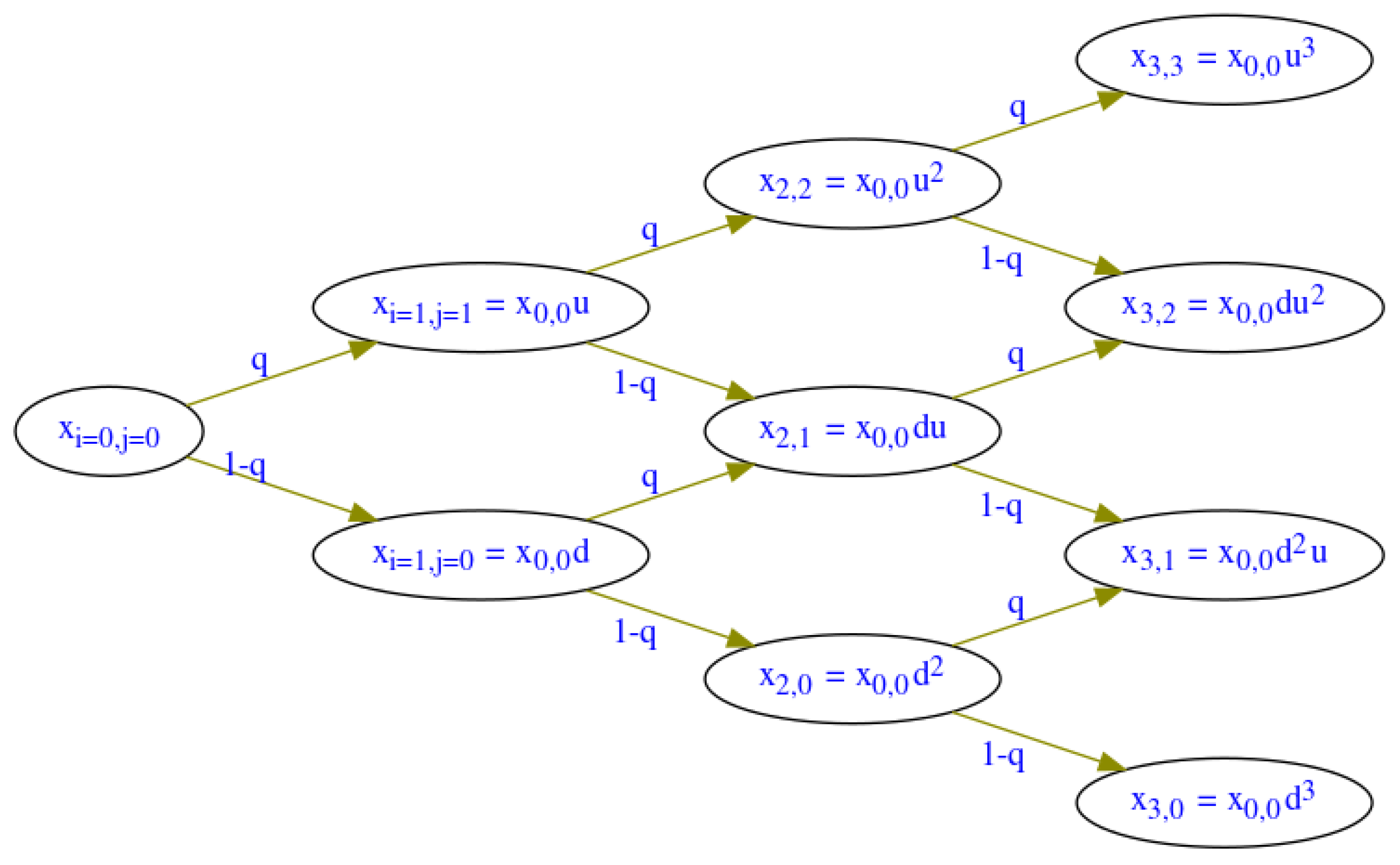
In BOPM, each node branches out into two distinct paths: one upward movement and the other a downward movement. Furthermore, $i=50$, denotes the total number of time steps in the model. In Table 1, the BOPM results are the exact solutions as a benchmark for comparing the results of the other two methods. The comparison shows that LSM and RL yield consistent results to BOPM, often matching to at least two decimal places.

In this study, the number of paths for training RL is 5000. In our experiments, we increased the number of paths to over 10,000 and up to 50,000; however, these modifications did not yield significant improvements in the results. Due to the stochastic nature of GBM during RL training, the RL results in Table 1 are the mean option prices of ten repetitions of the valuation process (for each case, the option is priced ten times, and the results are averaged). For LSM, the number of paths is 100,000, similar to Longstaff and Schwartz’s work [7].

5.2.2. Decision Boundary

In Table 1, the fair price of each option has been computed using the three methods. These three methods lead to slightly different values because their decision boundaries (the decisions to continue and exercise) are slightly different.

To delve into and understand this difference more, Figure 2 illustrates the decision boundary for the GBM price model with $S_0=36$, $\sigma =0.2$, and $K=40$. At any point in time (during the exercise window), if the price of the underlying asset is lower than the decision boundary curve, the option should be exercised. In Figure 2, the x-axis has been normalized (Time = t/Expiration Time), and the y-axis is the price of the underlying asset. The “locally jagged” nature of the decision boundary in the BOMP method is noteworthy. This boundary results from the discrete, stepwise structure of underlying asset price within the binomial lattice. The “diamond-like” local structure of these prices forms clusters, leading to jumps along the decision boundary curve, a phenomenon similarly discussed in [23].

Figure 2. Plot of decision boundaries for BOPM, LSM, and RL. The underlying asset is modeled using GBM with parameters (S₀ = 36, strike price = 40, volatility = 0.2).

5.2.3. Decision Frequency

In this section, we look into the frequency of exercise time for each method. The “frequency of exercise time” in this context is the distribution of exercise time (time of stopping) for 10,000 paths (generated from the GBM model), based on a method (LSM or RL).

Figure 3 shows the frequency of exercise time for the case where spot price $S_0=36$, strike price $K=40$, and volatility $\sigma =0.2$ are used in GBM. For example, at time step 5, the number of paths, for which the option is exercised, is around 500 for both LSM and RL. That is, for around 500 out of 10,000 paths (5%), LSM and RL suggest exercising the option at step 5.

Figure 3. Frequency of exercise time for LSM and RL. The underlying price model is GBM with $S_0=36$, $K=40$, and $\sigma =0.2$.

Note that in Figure 3, the bars after time step 50 represent the paths where the option is not exercised at the expiry time step or before (i.e., the option is never exercised). Both LSM and RL suggest not exercising the option at the expiry time step or before for around 25% of paths, leading to zero payoff for those paths.

LSM and RL lead to similar frequencies of exercise time in general, implying that RL can solve for a decision policy similar to LSM does.

We consider another case with larger uncertainty in the underlying asset prices over time, by using spot price $S_0=36$, strike price $K=40$, and volatility $\sigma =0.4$ in GBM. Figure 4 shows the resulting frequency of exercise time for each method. Compared to the case with volatility $\sigma =0.2$ (Figure 3), the frequencies of exercise time (Figure 4) are different.

Figure 4. Frequencies of exercise time for LSM and RL. $S_0=36$, $K=40$, and $\sigma =0.4$ in GBM.

For the case with $\sigma =0.4$ (Figure 4), RL leads to a different frequency of exercise time compared to LSM; especially for early time steps, RL does not suggest exercising the option before time step 24 for any path, whilst LSM suggests exercising the option before time step 24 for some paths. This behavior contrasts with Figure 3, where the RL and LSM methods exhibited similar frequencies of early exercises across all time steps.

5.2.4. How Well Does RL Decision Policy Improve Throughout Training?

Figure 5 shows the change in the frequency of exercise time for RL, indicating the evolution of RL decision policy throughout the training. At the beginning of the training, the weights are equal. As the training progresses (more batches), the weights converge to optimal values, and the decision policy also converges to the optimal one. The training is conducted with 5000 paths in five batches. As shown in Figure 5, the frequency of exercise time has almost no change after “Batch 2”, which indicates the decision policy converges to the optimal one. As explained in greater detail in the next subsection, the Option Value was computed after each batch and compared with the results from the BOMP method. If the final policy from the RL training resembles this value, it is considered an optimal policy.

Figure 5. Change in frequency of exercise time throughout RL training. $S_0=36$, $K=40$, and $\sigma =0.2$ in GBM.

5.2.5. How Option Values Change during Training?

Figure 6 shows the change in option value with each batch during the RL training process. In this example, the initial weights were set to ${\mathbf{w}}^{*}=[100,100,\dots 100]$. Subsequently, new weights are found in each batch. The new weights are then applied to a set of test paths to find the resulting option value option.

Figure 6. Change in Option Value following each batch during Reinforcement Learning training.

5.3. Option Price for GARCH Price Model

This section discusses the outcomes of implementing the two option valuation methods when the underlying price is modeled using the Generalized Autoregressive Conditional Heteroskedasticity (GARCH) model. The GARCH price model was selected to test the robustness of the RL method because GARCH is more complex and volatile than GBM. We calibrate the GARCH to historical Brent Crude Oil price data. In this section, Brent Crude Oil price acts as the Underlying Asset for the American Option. Subsequently, this calibrated GARCH model is utilized to simulate underlying asset price paths.

Note that BOMP is not applicable to GARCH, so only LSM and RL are implemented for the GARCH case. In addition, in this example, the strike price is $K=USD80$.

5.3.1. Hitorical Brent Crude Oil Price Data and GARCH Calibration

The historical Brent Crude Oil price data from 1987 to 2024, as shown in Figure 7, are used to calibrate the GARCH price model. Figure 8 contrasts the realized volatilities of the Brent Crude Oil price data and the forecasted volatilities of the calibrated GARCH model.

Figure 7. Historical Brent Crude Oil price data from 1987 to 2024.

Figure 8. Contrast of the realized volatilities of the Brent Crude Oil price data and the forecasted volatilities of the calibrated GARCH model.

5.3.2. Decision Boundary

The decision boundary curves solved using LSM and RL for the case with the calibrated GARCH price model are plotted in Figure 9. The decision boundary curves for the LSM and RL methods follow a similar trend, where the boundary curves at the expiry time $T=1$ approach the strike price ($K=USD80$).

Figure 9. Decision boundaries solved using LSM and RL for the case with calibrated GARCH price model. At any given time (x-axis), if the underlying asset price falls below the boundary, the option is to be exercised.

5.3.3. Decision Frequency

The resulting LSM and RL decision policies, as illustrated in Figure 9, are applied to 20,000 price paths sampled from the calibrated GARCH price model with the spot price $S_0=70$. The frequency of exercise time for each method is shown in Figure 10. Again, RL leads to a similar frequency of exercise time as LSM does. For approximately 7000 out of the 20,000 paths, LSM and RL suggest not exercising the option within the expiry time; in other words, the option is suggested to be exercised before/at the expiry time for around 14,000 paths.

Figure 10. Frequencies of exercise time for LSM and RL with the calibrated GARCH model.

5.3.4. How Well Does RL Decision Policy Improve Throughout Training?

Figure 11 shows the development of the frequency of exercise time, implying the development of the RL decision policy over the course of training. Initially (batch 0), the RL decision policy predominantly recommends exercising the option during the middle stages of the timeline (time steps between 15 and 30). However, with more batches of training, adjustments to the RL decision policy result in progressively fewer middle-stage exercises and more early-stage exercises. By the end of the fourth batch (Number 3 on the right side of Figure 11), the frequency of exercise time stabilizes, which indicates the RL decision policy converges.

Figure 11. Evolution of the frequency of exercise time throughout RL training batches.

5.3.5. Final Option Values

The two methods, RL and LSM, were used to find the decision boundary (policy) shown in Figure 9. The resulting decision boundaries from both methods were then tested on 10,000 paths to estimate the option value. Each method was repeated ten times to account for the stochastic nature of underlying price uncertainty (modeled by GARCH(1,1)). The average option value ($S_0=USD70$, $K=USD80$) was USD 10.75 for the RL method and USD 10.72 for the LSM method.

5.4. Option Price for EGARCH Price Model

This section discusses the implementation of RL and LSM methods for pricing AO, where the underlying price is modeled using the Exponential Generalized Autoregressive Conditional Heteroskedasticity (EGARCH) model. The EGARCH price model was selected since it can handle situations where negative returns increase future volatility more than positive returns. The GARCH model does not easily capture this feature. It makes EGARCH better suited for modeling real-world financial data where such asymmetry is common. We calibrate the EGARCH to historical Brent Crude Oil price data, the same as in the previous section. Subsequently, this calibrated EGARCH model is utilized to simulate underlying asset price paths.

5.4.1. EGARCH Price Model Calibration

Similar to the GARCH method, the Maximum Likelihood Estimation (MLE) method was used to estimate the parameters of the EGARCH model by calibrating it to oil price data (Figure 7). The estimated parameters of the EGARCH model are presented in Table 2. Figure 12 contrasts the realized volatilities of Brent Crude Oil price data with the forecasted volatilities from the calibrated EGARCH model. In Figure 12, the EGARCH(1,1,1) price model, due to its short memory (1,1,1), does not perfectly reconstruct the data. However, it is important to clarify that the primary focus of this paper is not on forecasting or developing models that perfectly fit the data. Rather, our work is centered on “Sequential Decision-Making” in American Options, where these models are used to simulate future paths as inputs to different pricing methods. Thus, even though the EGARCH(1,1,1) model may not reconstruct the data with high accuracy, it still serves as a consistent input for all methods under comparison.

Table 2. Parameter Values for the EGARCH model.

Parameter	Value
$\mu$	0.033
$\omega$	0.030
$\alpha$	0.188
$\gamma$	−0.038
$\beta$	0.985

Figure 12. Contrast of the realized volatilities of the Brent Crude Oil price data and the forecasted volatilities of the calibrated EGARCH model.

5.4.2. Decision Boundary

The decision boundary curves solved using LSM and RL for the case with the calibrated EGARCH price model are plotted in Figure 13. A notable difference between these boundaries is that the RL method results in “more” early exercises before half the expiry date. In contrast, the LSM method has a lower value boundary ($t<T/2$), resulting in fewer paths below this value and, consequently, “fewer” early exercises.

Figure 13. Decision boundaries solved using LSM and RL for the case with calibrated EGARCH price model.

5.4.3. Decision Frequency

The resulting decision policies using LSM and RL, illustrated in Figure 13, were applied to 10,000 price paths sampled from the calibrated EGARCH price model with a spot price of $S_0=USD70$ and strike price $K=USD80$. The frequency of exercise times for each method is shown in Figure 14. In both methods, approximately 35% of the paths are not exercised early. However, the RL method exhibits more early exercises before time step 25, as indicated by its decision boundary (discussed in the previous section).

Figure 14. Frequencies of exercise time for LSM and RL with the calibrated EGARCH model.

5.4.4. Final Option Values

The two methods, RL and LSM, were used to find the decision boundary (policy) shown in Figure 13. The decision boundaries obtained from both methods were then tested on 10,000 paths to estimate the option value. Each method was repeated ten times to account for the stochastic nature of underlying price uncertainty, modeled by EGARCH(1,1,1). The average option value, with $S_0=USD70$, strike price = USD 80 was USD 15.01 for the RL method and USD 14.91 for the LSM method.

6. Discussion

The classical LSM method is based on a predefined probabilistic model of an underlying asset price. The LSM samples future paths of the underlying asset price from the predefined probabilistic model, estimates conditional expected values using regression, and derives the option value through backward induction.

Conversely, the Reinforcement Learning (RL) approach is model free, eliminating the need for a predefined probabilistic price model to value an option. Instead, RL can utilize historical underlying asset price data to train for the optimal decision policy, exemplifying a data-driven approach to pricing American Options. Our study demonstrates that the RL method is effective for valuing American Options and yields results comparable to those obtained using the BOPM and LSM methods.

A limitation of the RL method needs to be mentioned. The stability of the training process can be an issue in finding the optimal policy. Careful attention is required when designing the RL algorithm with the appropriate number of batches, iterations, and learning rates to avoid overfitting and underfitting.

Future work could explore the potential of different feature functions (in this study only Laguerre was considered) in improving policy and valuation of the American Option. Additionally, investigating other types of underlying price models, such as jump models or two-factor models, could provide further insight.

7. Conclusions

Identifying the optimal exercise time of an American Option is a Sequential Decision-Making problem. At each time step, the option holder must decide whether to exercise the option based on the immediate reward or wait for potential future rewards, considering downstream uncertainties and decisions.

Our analysis shows that decision boundaries derived from the Least Squares Method Monte Carlo (LSM) method tend to be non-smooth. Notably, for the EGARCH(1,1,1) price model, the decision boundary changes abruptly at certain time steps when the number of sampled prices in the training set is around 100,000 paths. This occurs because LSM performs regression at each time step, whereas RL embeds time (t) directly within the Q-value function. A further conclusion is that, in the EGARCH (1,1,1) model, the LSM and RL-based methods result in two different exercise policies. However, as demonstrated in Section 5.4.4, applying these different final policies to test paths yields the same option valuation. Despite the different exercise policies, the final option values are identical. This contrasts with the cases of the GBM and GARCH (1,1) models, where both the final policies and the option values are similar.

Finally, the Reinforcement Learning (RL) method learns policies through an iterative process. During this learning process, an iteration step where policy “change” stops is observed, indicating convergence. In this work, by employing the experience-replay method in RL, convergence is achieved within a few batches. The key contributions of this work can be summarized as follows: (a) The implementation, illustration, comparison, and discussion of the three methods—BOPM, LSM, and RL—for valuing American Options in cases with constant and stochastic volatility models—GBM and GARCH—of underlying asset price uncertainty. (b) The study and evaluation of an RL implementation for Sequential Decision-Making sheds light on how learning in RL contributes to improving “decisions”. (c) The authors of [7] presented twenty different GBM-based models and used the LSM technique to determine option values. In this work, we apply the RL method to the same models, as shown in Table 1, and compare it with the LSM approach.