A Multi-Strategy Improved Honey Badger Algorithm for Engineering Design Problems

Abstract

A multi-strategy improved honey badger algorithm (MIHBA) is proposed to address the problem that the honey badger algorithm may fall into local optimum and premature convergence when dealing with complex optimization problems. By introducing Halton sequences to initialize the population, the diversity of the population is enhanced, and premature convergence is effectively avoided. The dynamic density factor of water waves is added to improve the search efficiency of the algorithm in the solution space. Lens opposition learning based on the principle of lens imaging is also introduced to enhance the ability of the algorithm to get rid of local optimums. MIHBA achieves the best ranking in 23 test functions and 4 engineering design problems. The improvement of this paper improves the convergence speed and accuracy of the algorithm, enhances the adaptability and solving ability of the algorithm to complex functions, and provides new ideas for solving complex engineering design problems.

1. Introduction

Optimization problems are ubiquitous in the field of engineering design, from mechanical design to structural engineering to electronic system design, where engineers often need to find optimal solutions under multiple design variables and constraints [1]. Traditional optimization methods, such as gradient descent [2] and Newton’s method [3], are often difficult to cope with complex, multi-peak, and high-dimensional engineering design problems. In recent years, biologically inspired optimization algorithms, such as parrot optimizer (PO) [4], coati optimization algorithm (COA) [5], and snow ablation optimizer (SAO) [6], have attracted extensive attention for their efficiency and robustness in dealing with complex problems.

The hippo optimization algorithm (HO) proposed by Mohammad Hussein Amiri et al. mimics hippopotamus’ defense and predator evasion behaviors, demonstrates strong global search and local exploitation capabilities, and effectively solves four different engineering design challenges [7]. Jun Wang et al. proposed the black-winged kite optimization algorithm (BKA), which is inspired from the predatory and migratory behaviors of the black-winged kite, has significant evolutionary and searching capabilities, and shows great advantages in engineering design problems [8]. The multi-strategies improved beluga whale optimization algorithm (MSBWO), proposed by Zhaoyong Fan et al., improves the algorithm’s global search capability and convergence speed by introducing improvements such as chaos mapping initialization, elite pooling strategy, and adaptive lévy flight [9]. Mahdi Azizi et al. proposed the energy valley optimization (EVO) algorithm, inspired by the principles of stability and particle decay in the field of physics. EVO is effective and superior in solving complex optimization problems [10]. The gold rush optimization algorithm (GRO) proposed by Zolfi Kamran is inspired by the behavior of gold prospectors exploring for gold, and GRO searches for an optimal solution by simulating the three key processes of migration, collaboration, and panning for gold. The application of the GRO algorithm to several benchmark test functions and real-world engineering problems has shown that it has significant advantages in global search and engineering optimization problems [11]. In addition, Peng Wang et al. proposed a quantum intelligent optimization algorithm framework for quantum intelligent computation of global optimization problems, as well as a quantum multi-objective optimization learning model and deep neural network architecture search and parameter optimization techniques for quantum intelligent optimization [12]. The zebra optimization algorithm (ZOA), proposed by Eva Trojovská et al., is inspired by the foraging and defensive behaviors of zebras, and is applied to a wide range of optimization problems with different exploration and development requirements [13]. Mohamed Abdel-Basset et al. proposed the nutcracker optimization algorithm (NOA) to mimic the behavior of a nutcracker for solving global optimization and engineering design problems [14]. Laith Abualigah et al. proposed a Reptile Search Algorithm (RSA), inspired by crocodile hunting behavior. They introduced two mathematical models for updating the location of candidate solutions, and implemented four metrics to qualitatively study the proposed RSA [15]. Amin Abdollahi Dehkordi et al. proposed nonlinear-based chaotic Harris Hawks optimization (NCHHO), which uses chaotic and nonlinear control parameters to improve the optimization performance of HHO and solve the Internet of Vehicles routing problem [16]. Bibekananda Jena et al. submitted a new hybrid differential squirrel search algorithm optimization algorithm (DSSE) for solving global optimization difficulties by combining the search methodology of the squirrel search algorithm with the differential evolutionary optimization process [17]. Afshin Faramarzi et al. developed a novel optimization algorithm called the Equilibrium Optimizer (EO), inspired by the mass balance model, where the algorithm design includes highly exploratory and exploitative search mechanisms to stochastically change the solution [18]. The multipopulation ensemble particle swarm optimizer (MPEPSO) algorithm, proposed by Ziang Liu et al., enhances the efficiency and accuracy of the algorithm by combining different PSO search strategies and dynamically adjusting the allocation of reward subpopulations, which better solves the engineering design problems [19]. Weiguo Zhao et al. modeled three unique foraging strategies of manta rays and developed Manta ray foraging optimization (MRFO), an algorithm with few adjustable parameters that is easy to implement [20]. These algorithms show great potential and application in the field of engineering design. honey badger algorithm (HBA), as an emerging optimization algorithm, provides new ideas for solving engineering design problems with its unique search mechanism and powerful global search capability [21].

Ajay Kumar Bansal et al. optimized HNGS, a hybrid nano grid system for the future residential area of Mahendragarh, Haryana, India, using honey badger algorithm (HBA) and obtained a higher quality solution [22]. Rajendran Arul Jose et al. combined the HBA with a gradient boosting decision tree (GBDT) to improve the prediction accuracy of the control parameters and to realize the real-time adjustment of the parameters to meet the changes in the grid demand [23]. Allan J Wilson et al. proposed an optimization framework based on binarized spiking neural network (BzSpNN) and honey badger algorithm for cluster head selection in WSNs to minimize the energy consumption and extend the network life cycle [24]. Meng Jiang et al. proposed a combined method (CGH-GTO), based on the improved gray wolf optimizer (IGWO), honey badger algorithm (HBA), and gorilla troops optimizer (GTO), for the identification of PV model parameters [25]. Xinyu Ren et al. constructed a two-layer planning model for combined cooling, heating and power (CCHP) and developed the multi-objective honey badger algorithm (MOHBA), which improves the economic, energy, and environmental performance of the CCHP system [26]. Boxiong Wang et al. proposed an improved binary honey badger algorithm for IoT traffic datasets based on lévy flights, which improves the performance of HBA for IoT device identification in the feature selection problem [27]. Siwen Zhang et al. proposed α4CycρHBA, an algorithm that significantly improves the global search capability and convergence speed by introducing density factors based on primitive functions and mathematical spirals in polar coordinate systems [28]. Peixin Huang et al. proposed an improved honey badger algorithm called ODEHBA, which excels in solving complex numerical problems, engineering design problems, and routing problems for vehicular networking [29]. Jinrui Zhang et al. proposed a back propagation neural network (BPNN) model based on HBA optimization for predicting the migration time of toxic fumes induced by blasting in underground mines to further guide and improve the ventilation design [30]. The honey badger algorithm excels in solving optimization problems with its simplicity and efficiency, and is especially suitable for complex and high-dimensional search spaces. Although the HBA shows some advantages in optimization problems with its simple structure and clear ideas, it also has some drawbacks. The HBA is weak in exploration capability, which leads to the algorithm’s difficulty in effectively exploring the solution space at the early stage of the search, thus affecting the ability of global optimization search. The algorithm does not handle the balance between exploration and exploitation well enough, which modifies the convergence performance of the algorithm and the quality of the final solution. The HBA also tends to fall into local optimal solutions, and it requires more iterations to achieve better optimization results, which is a challenge to the computational resources. In order to better solve the engineering design problem, this paper improves the original HBA.

In this paper, we propose an improved honey badger algorithm (MIHBA) based on multiple strategies to address the shortcomings of the honey badger algorithm. The introduction of Halton sequence to initialize the population enables the generation of point sets that are uniformly distributed in multidimensional space. Initializing the population with Halton sequence can improve the diversity of the algorithm and avoid premature convergence. The dynamic density factor of water waves is introduced to perform an efficient search in the solution space by modeling the propagation, refraction, and breaking wave motion mechanisms of water waves. Introducing the dynamic density factor of water waves into HBA can enhance the global search ability and local search ability of the algorithm, thus improving the convergence speed and the quality of the algorithm. Lens opposition-based learning is introduced to enhance the search capability of the algorithm by introducing this new mechanism for escaping local optima. This approach helps the algorithm to jump out when it falls into a local optimum and continue the search towards the global optimum solution. The main contributions of this paper are as follows:

• The introduction of Halton sequence to initialize the population improves the initial diversity of the population and helps to avoid early convergence of the algorithm to local optimal solutions;
• The combination of the dynamic density factor of the water waves allows the algorithm to explore a wider search range and improves the adaptability and solving ability for complex functions;
• The learning strategy based on the lens imaging principle improves the ability of the algorithm to escape from local optimal solutions and enhances the global search capability;
• The proposed algorithm is tested for performance on 23 benchmark test functions and applied to four engineering design problems, where the algorithm shows great advantages.

2. Algorithm Design

2.1. Honey Badger Algorithm

The honey badger algorithm (HBA) is a meta-heuristic algorithm that solves optimization problems by simulating the dynamic search behavior of the honey badger foraging. The main steps of the HBA include initialization, defining and updating the density factor, the mining phase, and the honey harvesting phase.

In the initialization phase, the algorithm performs an initialization operation on the number $N$ of the honey badger population within the set boundaries, as shown in Equation (1).

$$X_i=l{b}_i+r_1\cdot \left(u{b}_i-l{b}_i\right),r_1\in \left(0,1\right),$$

(1)

where $X_i$ is the location of the $ith$ individual of the $N$ candidate individuals, and the upper and lower bounds of the search space are denoted by $ub$ and $lb$, respectively.

The strength of the honey badger’s sense of smell is related to prey concentration and the distance between prey. Let $I$ be the odor intensity of the prey, if the honey badger moves quickly when it smells the food odor very high, as shown in Equation (2).

$$\{\begin{array}{l}{I}_i=r_2\cdot S/\left(4\pi d_i^2\right),r_2\in \left(0,1\right)\\ S={\left(x_i-x_{i+1}\right)}^2\\ d_i=x_{prey}-x_i\end{array},$$

(2)

where $S$ represents the source strength, $d_i$ represents the distance between the current honey badger individual and the target prey, and $r_2$ is a random number between (0, 1).

The density factor controls the time-varying randomization and ensures the balance between the exploration phase and the development phase, defined as shown in Equation (3).

$$\partial =C\times \exp \left(-t/t_{\max }\right),$$

(3)

where $t$ is the current number of iterations, $t_{\max }$ is the maximum number of iterations, $C\ge 1$, and the default value is 2.

During the digging phase, honey badgers use the strength of their sense of smell to locate and dig for prey. During this phase, the honey badger’s locomotor behavior resembles a heart curve, and the locomotor map simulation is shown in Equation (4).

$$x_{new}=x_{prey}+F\cdot \beta \cdot I\cdot x_{prey}+F\cdot r_3\cdot d_i\cdot \left|\cos \left(2\pi r_4\right)\cdot \left[1-\cos \left(2\pi r_5\right)\right]\right|,$$

(4)

where $x_{new}$ represents the updated position and $x_{prey}$ is the global optimal position in the current state. $\beta$ represents the ability of the honey badger to hunt, and its default value is 6. $r_3$, $r_4$, $r_5$ are three random numbers between (0, 1). In addition, $F$ denotes the flag that controls the search direction, as determined by Equation (5):

$$F=\{\begin{array}{l}1,if\begin{array}{c}\end{array}{r}_6\le 0.5\\ -1,otherwise\end{array}.$$

(5)

While in the honey phase, the honey badger follows the guide bird to find the hive, this phase is similar to the local search in the algorithm, simulated as in Equation (6).

$$x_{new}=x_{prey}+F\cdot r_7\cdot \partial \cdot d_i,r_7\in \left(0,1\right).$$

(6)

2.2. Proposed Algorithm

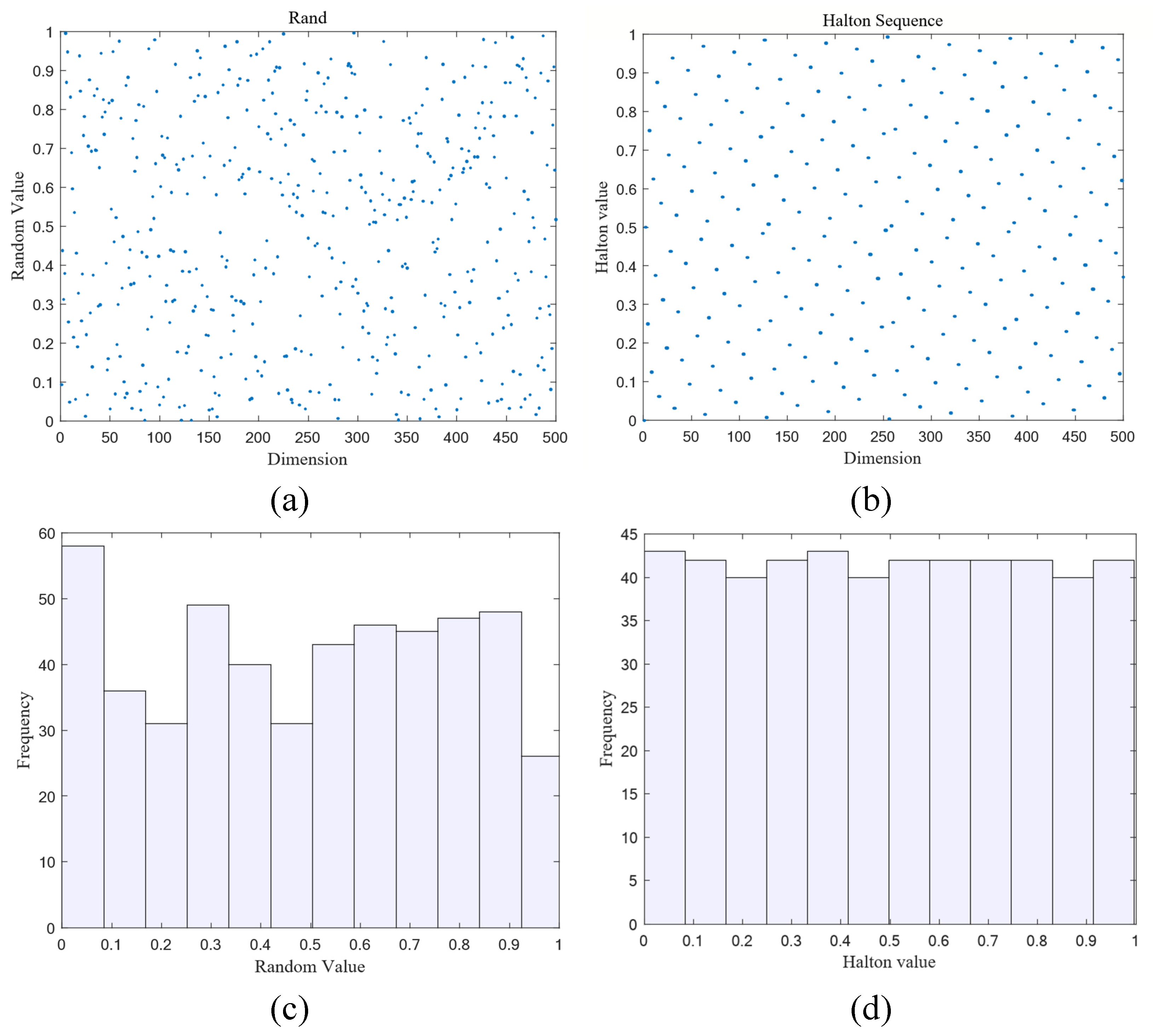
2.2.1. Halton Sequence Initializes the Population

In the original honey badger algorithm, a highly random population was obtained by randomly initializing the population using the rand function. However, this randomization does not necessarily ensure that individuals are uniformly distributed throughout the solution space, which may lead to a slow population search, as well as reduce the diversity of the algorithms. To solve this problem, this paper introduces Halton sequence to generate pseudo-random numbers to initialize the population [31]. The pseudo-randomness of the Halton sequence ensures that the individuals are more evenly distributed throughout the solution space, thus increasing the diversity of the initialization phase of the algorithm. This helps the individual to quickly discover the location of high-quality solutions, speeds up the convergence of the algorithm, and improves the convergence accuracy of the algorithm.

The two-dimensional Halton sequence is realized by selecting two primes as the basis quantities and forming a series of uniformly distributed and non-repeating points by constant slicing of these two basis quantities. This slicing process can be described by a mathematical model as described in Equations (7)–(9).

$$n={\displaystyle \sum _{\mathrm{i}=0}^{\mathrm{m}}{b}_i}\times p^i=b_m\times p^m+L+b_1\times p^1+b_0,$$

(7)

$$\theta \left(n\right)=b_0{p}^{-1}+b_1{p}^{-2}+L+b_m{p}^{-m-1},$$

(8)

$$H\left(n\right)=\left[q_1\left(n\right),q_2\left(n\right)\right],$$

(9)

where $n\in [1,N]$ is any integer, $p$ is a prime number greater than or equal to 2, denoted by the underlying quantity of the Halton sequence, $b_i\in \{0,1,2,\cdots ,p-1\}$ is a constant, $\theta \left(n\right)$ is a defined sequence function, and $H\left(n\right)$ is the resulting Halton sequence. This sequence replaces Equation (1) of the original algorithm for population initialization. As shown in Figure 1, where Figure 1a shows random distribution map, Figure 1b shows Halton distribution map, and Figure 1c,d show the histograms of particle distributions corresponding to the two initializations, respectively. According to Figure 1, it can be clearly seen that the Halton initialization possesses a more uniform particle distribution than the random initialization.

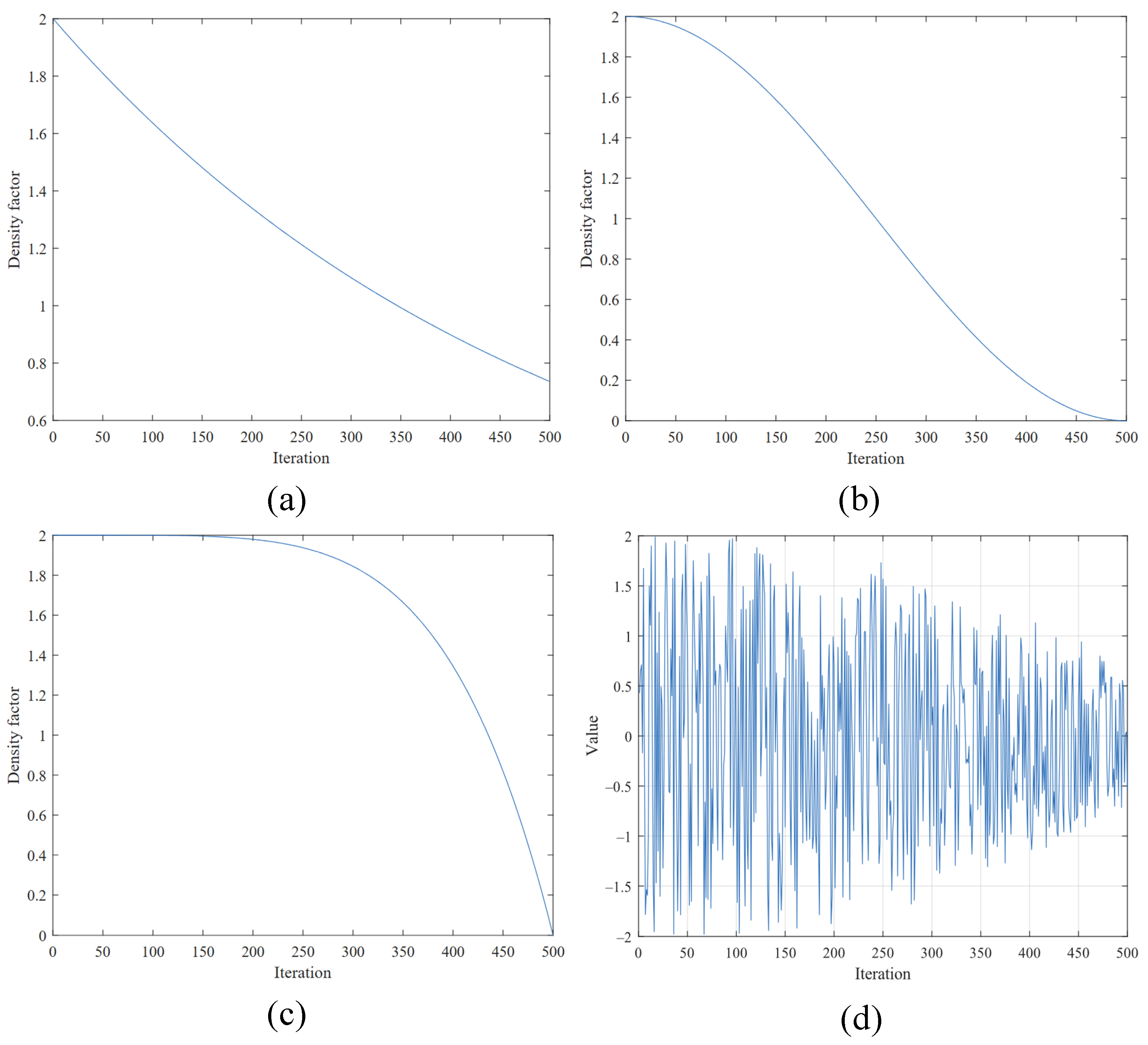
2.2.2. Water Wave Dynamic Density Factor

In HBA, the value of the density factor $\partial$ controls the balance of the algorithm during the exploration and development phases. The primitive decreasing mechanism often leads the algorithm to fall into a local optimum, making it difficult to effectively cover and explore the entire search space, thus limiting the accuracy of the algorithm in the development stage, especially when dealing with complex and high-dimensional problems. To solve this problem, researchers have proposed a variety of improved convergence factors: reference [32] proposes a convergence factor based on sinusoidal functions, which can help the algorithm to search for the optimal value in the global range, as shown in Equation (10). Reference [33] presents the power-of-five nonlinear convergence factor, which can enhance the search ability of the algorithm, as shown in Equation (11). Reference [34] proposes a convergence factor that utilizes the uncertainty property in water wave dynamics, which improves the algorithm’s adaptability and solving ability for complex functions, as shown in Equation (12). Figure 2 illustrates the above four convergence factors, where (a) is the original convergence factor shown in Equation (3), (b) is the sinusoidal convergence factor shown in Equation (10), (c) is the power-of-five convergence factor demonstrated in Equation (11), and (d) is the water wave dynamic density factor shown in Equation (12).

$$\partial =1+\sin \left(\pi /2+\pi \times t/t_{\max }\right),$$

(10)

$$\partial =2-2\times {\left(t/t_{\max }\right)}^5,$$

(11)

$$\partial =2\times rand\times S\times \exp {\left(-t/t_{\max }\right)}^3,$$

(12)

where $t_{\max }$ is the maximum number of iterations, $t$ is the current number of iterations, $S$ is a random integer, and $S\in \left[0,1\right]$.

HBA often lacks accuracy when dealing with complex multimodal functions. To solve this problem, the dynamic density factor of water waves is introduced. The uncertain fluctuation characteristics in the water wave dynamics can dynamically adjust the density factor, realizing the adaptive switching of the algorithm between the exploration and development phases. This self-adjustment mechanism helps to improve the overall search efficiency of the algorithm and avoid falling into local optimization. The multi-wave interference characteristic in water wave dynamics is very similar to the characteristics of complex multi-peak optimization problems. Using this characteristic to design the density factor helps the algorithm to better cope with the complex multi-peak problem and reduce the risk of falling into the local optimum. Compared with the traditional methods, such as sinusoidal function and power-of-five convergence factor, the water wave dynamics density factor can better capture the uncertainty characteristics in the complex environment, realize the adaptive equilibrium of exploration and development, enhance the ability to cope with the complex multi-peak problems, and improve the adaptability of the algorithm in the complex environment.

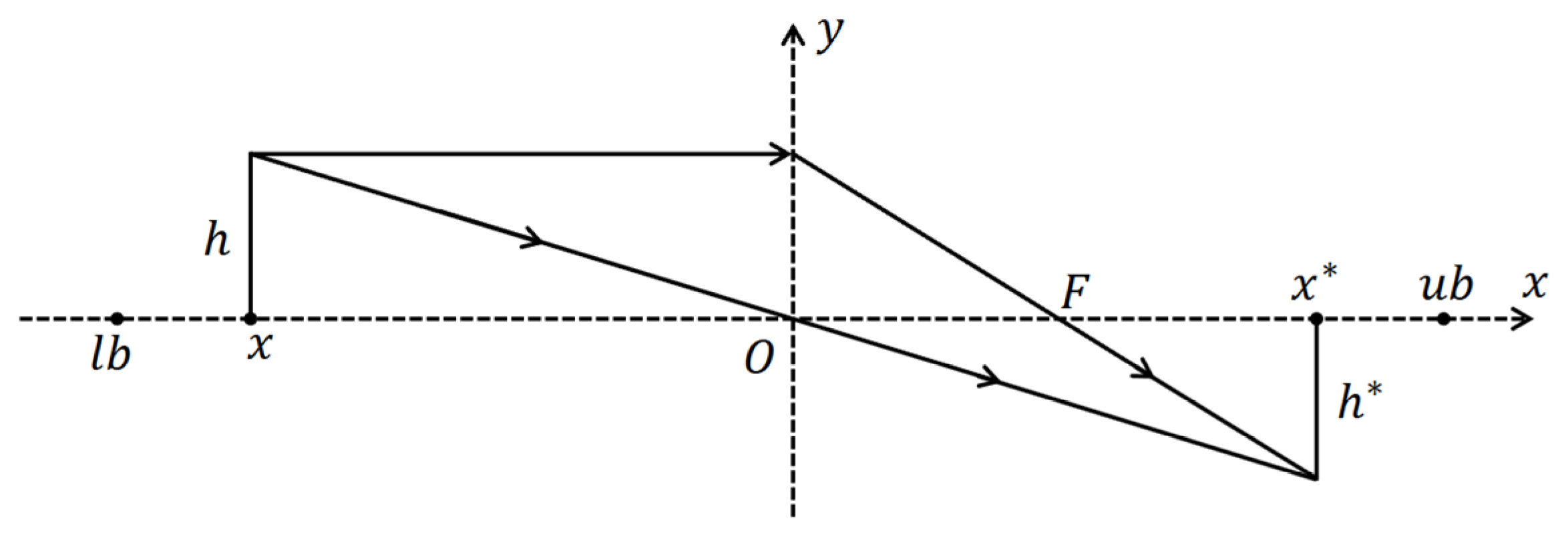
2.2.3. Lens Opposition-Based Learning

Lens opposition-based learning (LOBL) [35] incorporates the concepts of opposition-based learning (OBL) [36] and the scientific principles of lens imaging, aiming to improve the search capabilities of the algorithm. The LOBL strategy skillfully draws on the dyadic nature and the principle of focus imaging in optical systems and exhibits more efficient performance than OBL in finding optimal or near-optimal solutions.

In optical imaging, if an object is placed beyond twice the focal length of the lens, an inverted and reduced-size solid image is formed on the opposite side of the lens, between one and two times the focal length. As shown in Figure 3, the midpoint of the $[lb,ub]$ interval is $O$. Consider the $y$-axis as a convex lens. An object of height $h$ is located at point $x$. Point $x$ is at twice the focal length of the lens. When this object is imaged through a lens, the coordinates of the vertices of its image will become $\left(x^{*},h^{*}\right)$. The detailed mathematical Equation (13) is shown.

$$((lb+ub)/2-x)/\left(x^{*}-(lb+ub)/2\right)=h/h^{*}.$$

(13)

Setting $k=\left(h/h^{*}\right)$, Equation (13) can be simplified to Equation (14).

$$x^{*}=\left(lb+ub\right)/2+\left(lb+ub\right)/2k-x/k,$$

(14)

where $k$ is a dynamically varying coefficient that increases with the number of iterations $t$. The rate of increase is controlled by ${\left(t_c/t_{\max }\right)}^{1/2}$ and scaled up to the 10th power to simulate the focusing effect of the lens as shown in Equation (15). Pos(t + 1) is the new position as shown in Equation (16).

k = (1 + (t_c/t_max)^1/2)¹⁰,

(15)

$$x_{new}(t+1)=(lb+ub)/2+(lb+ub)/(2\times k)-\left(x_{prey}(t)/k\right),$$

(16)

where $t_{\max }$ is the maximum number of iterations, $t$ is the current number of iterations, $x_{prey}$ is the position of the current individual, $x_{new}$ is the updated position, and $ub$ and $lb$ are the upper and lower bounds, respectively.

The benefit of introducing LOBL is that it is able to utilize the geometric relationship between the current solution and the optimal solution instead of a completely random search, which helps to improve the global exploration capability of the algorithm. By dynamically adjusting the parameters, a balance between exploration and exploitation can be achieved, thus improving the convergence speed and stability of the algorithm. The new solution updating mechanism can better utilize the geometric properties of the problem itself and improve the solution accuracy of the algorithm. And the adaptive adjustment capability of the update strategy for the dynamic density factor of water waves can dynamically adjust the algorithm behavior according to the problem characteristics. There is complementarity between the two update strategies, which can improve the overall optimization performance. The overall flowchart of the algorithm is shown in Figure 4.

The pseudocode of the algorithm is shown below (Algorithm 1).

Algorithm 1. Pseudo code of MIHBA

$\mathrm{Set}\mathrm{initial}\mathrm{parameters}{t}_{\max }$, $N$, $\beta$, $C$.

Initialize the population positions using the Halton mapping as shown in Equations (7)–(9).

$\mathrm{Evaluate}\mathrm{the}\mathrm{fitness}\mathrm{of}\mathrm{each}\mathrm{honey}\mathrm{badger}\mathrm{position}{x}_i$$\mathrm{using}\mathrm{objective}\mathrm{function}\mathrm{and}\mathrm{assign}\mathrm{to}{f}_i$$,i\in \left[1,2,\dots ,N\right]$.

$\mathrm{Save}\mathrm{best}\mathrm{position}{x}_{prey}$$\mathrm{and}\mathrm{assign}\mathrm{fitness}\mathrm{to}{f}_{prey}$.

$\mathbf{while}t\le t_{\max }$ do

Update the decreasing factor $\alpha$ using Equation (12).

$\mathbf{for}i=1$ to $N$ do

$\mathrm{Calculate}\mathrm{the}\mathrm{intensity}{I}_i$ using Equation (2).

$\mathbf{if}r<0.5$ then

$\mathrm{Update}\mathrm{the}\mathrm{position}{x}_{new}$ using Equation (4).

Else

Update the position using Equation (6).

end if

Update the global best position using the lens opposition-based learning as described in Equation (16).

$\mathbf{if}{f}_{new}\le f_i$ then

$\mathrm{Set}{x}_i=x_{new}$$\mathrm{and}{f}_i=f_{new}$.

end if

$\mathbf{if}{f}_{new}\le f_{prey}$ then

$\mathrm{Set}{x}_{prey}=x_{new}$$\mathrm{and}{f}_{prey}=f_{new}$.

end if

end for

end while Stop criteria satisfied.

$\mathbf{Return}{x}_{prey}$

2.3. Subsection

2.3.1. Time Complexity

The algorithm time complexity mainly depends on the population size $N$ and the dimension of the problem $Dim$, and the time complexity of Halton mapping is $O\left(N\times dim\right)$. In each iteration, the position update of each individual requires the computation of a new density factor $\alpha$ and a new position $X_{new}$. The time complexity of this part mainly depends on the population size $N$, the dimension $Dim$, and the complexity of computing $\alpha$ and $X_{new}$. The time complexity of computing α is $O\left(1\right)$ because it involves simple operations on the number of constants. The time complexity of updating X_new is $O\left(dim\right)$ because it needs to be computed for each dimension. Therefore, the total time complexity of each iteration is $O\left(N\times dim\right)$. This strategy updates the global optimal position at the end of each iteration, and its time complexity is $O\left(dim\right)$ because it needs to be computed for each dimension.

Therefore, the time complexity of MIHBA is $O\left(t_{max}\times N\times dim\right)$, which is equal to the time complexity of the HBA.

2.3.2. Space Complexity

Space complexity is a key measure of the storage space required for an algorithm to run. The storage of the honey badger population location X requires $N\times dim$ spatial units. The MIHBA also needs to store variables such as the global optimal position $X_{prey}$, the fitness, the current number of iterations $t$, etc., which require $O\left(dim\right)$ space. The density factor $\alpha$ and other temporary variables require $O\left(1\right)$ space. Thus, the overall space complexity of the algorithm, $O\left(N\times dim\right)$, is equal to that of the original HBA. As a result, MIHBA did not add additional storage space requirements.

3. Experiments

In order to examine the performance of the improved HBA, this study evaluated the MIHBA on 23 standard test functions. These test functions were grouped into 3 categories: single-peak functions, multimodal functions, and fixed-dimension functions. Finally, the MIHBA was subjected to ablation experiments and compared with five meta-heuristics.

3.1. Experimental Setup and Evaluation Criteria

To ensure the accuracy and reproducibility of the experiments, all tests were conducted in the same environment. The experimental environment was configured with a Windows 10 operating system, an Intel^® Core™ i5-12490F 3.0 GHz processor, and 16 GB of operating memory. All algorithms were implemented and tested in the MATLAB R2020b programming environment. All benchmark functions are shown in

Table 1. Benchmark functions.

Function	Dimension	Domain	Theoretical Optimum
$f_1(x)={\displaystyle {\sum }_{i=1}^n{x}_i^2}$	30	[−100, 100]	0
$f_2(x)={\displaystyle {\sum }_{i=1}^n\left|x_i\right|+{\displaystyle {\prod }_{i=1}^n\left|x_i\right|}}$	30	[−10, 10]	0
$f_3(x)={\displaystyle {\sum }_{i=0}^{n-1}{\left\{{\displaystyle {\sum }_{j=0}^{j<i}{x}_i}\right\}}^2}$	30	[−100, 100]	0
$f_4(x)={\max }_i\left\{\left|x_i\right|,1\le i\le n\right\}$	30	[−100, 100]	0
$f_5(x)={\displaystyle {\sum }_{i=1}^{n-1}\left[100{\left(x_{i+1}-x_i^2\right)}^2+{\left(x_i-1\right)}^2\right]}$	30	[−30, 30]	0
$f_6(x)={{\displaystyle {\sum }_{i=1}^n\left(\left[x_i+0.5\right]\right)}}^2$	30	[−100, 100]	0
$f_7(x)={\displaystyle {\sum }_{i=1}^{n}i{x}_i^4}+random\left[0,1\right)$	30	[−1.28, 1.28]	0
$f_8(x)={\displaystyle {\sum }_{i=1}^n-xi\sin \left(\sqrt{\left|x_i\right|}\right)}$	30	[−500, 500]	−12,569.4
$f_9(x)={\displaystyle {\sum }_{i=1}^n\left[x_i^2-10\cos \left(2\pi x_i\right)+10\right]}$	30	[−5.12, 5.12]	0
$\begin{array}{ll}{f}_{10}(x)=& -20\exp \left(-0.2\sqrt{\left(1/n\right)\times {\displaystyle {\sum }_{i=1}^n{x}_i^2}}\right)\\ & -\exp \left(\left(1/n\right)\times {\displaystyle {\sum }_{i=1}^n\cos \left(2\pi x_i\right)}\right)+20+e\end{array}$	30	[−32, 32]	0
$f_{11}=\left(1/4000\right)\times {\sum }_{i=1}^n{x}_i^2-{\prod }_{i=1}^n\cos \left(x_i/\sqrt{x+1}\right)+1$	30	[−600, 600]	0
$\begin{array}{l}{f}_{12}(x)=\left(\pi /n\right)\times \{10\sin \left(\pi y_1\right)+{\left(y_n-1\right)}^2\\ +{\displaystyle {\sum }_{i=1}^{n-1}{\left(y_i-1\right)}^2\left[1+10{\sin }^2\left(\pi y_{i+1}\right)\right]}\}\\ y_i=1+\left(x_i+1\right)/4\\ u\left(x_i,a,k,m\right)=\{\begin{array}{cc}k{\left(x_i-a\right)}^m& x_i>a\\ 0& -a<x_i<1\\ k{\left(-x_i-a\right)}^m& x_i<-a\end{array}\end{array}$	30	[−50, 50]	0
$\begin{array}{ll}{f}_{13}(x)=& 0.1\{{\displaystyle {\sum }_{i=1}^n{\left(x_i-1\right)}^2\left[1+{\sin }^2\left(3\pi x_1+1\right)\right]}\\ & {\sin }^2\left(3\pi x_1\right)+{\left(x_n-1\right)}^2\left[1+{\sin }^2\left(2\pi x_{ni}\right)\right]\}\\ & +{\displaystyle {\sum }_{i=1}^{n}u\left(x_i,5,100,4\right)}\end{array}$	30	[−50, 50]	0
$f_{14}(x)={\left(1/500+{\sum }_{j=1}^{25}\left(1/\left(j+{\displaystyle {\sum }_{i=1}^2{\left(x_i-a_{ij}\right)}^6}\right)\right)\right)}^{-1}$	2	[−65, 65]	1
$f_{15}(x)={{\displaystyle {\sum }_{i=1}^{11}\left[a_i-x_1\left(b_i^2+b_i{x}_2\right)/\left(b_i^2+b_i{x}_3+x_4\right)\right]}}^2$	4	[−5, 5]	0.00003075
$f_{16}(x)=4x_1^2-2.1x_1^4+x_1^6/3+x_1{x}_2-4x_2^2+4x_2^4$	2	[−5, 5]	−1.0316285
$\begin{array}{ll}{f}_{17}(x)=& {\left(x_2-\left(5.1/4{\pi }^2\right)x_1^2+\left(5/\pi \right)x_1-6\right)}^2\\ & +10\left(1-\left(1/8\pi \right)\right)\cos x_1+10\end{array}$	2	[−5, 5]	0.398
$\begin{array}{ll}{f}_{18}(x)=& \left[1+{\left(x_1+x_2+1\right)}^2\times \left(19-14x_1+3x_1^2-14x_2+6x_1{x}_2+3x_2^2\right)\right]\\ & \cdot \left[30+{\left(2x_1-3x_2\right)}^2\times \left(18-32x_1+12x_1^2+48x_2-36x_1{x}_2+27x_2^2\right)\right]\end{array}$	2	[−2, 2]	3
$f_{19}(x)=-{\displaystyle {\sum }_{i=1}^4{c}_i\exp \left(-{\displaystyle {\sum }_{j=1}^3{a}_{ij}{\left(x_j-p_{ij}\right)}^2}\right)}$	3	[0, 1]	−3.86
$f_{20}(x)=-{\displaystyle {\sum }_{i=1}^4{c}_i\exp \left(-{\displaystyle {\sum }_{j=1}^6{a}_{ij}{\left(x_j-p_{ij}\right)}^2}\right)}$	6	[0, 1]	−3.32
$f_{21}(x)=-{{\displaystyle {\sum }_{i=1}^5\left[\left(x-a_i\right){\left(x-a_i\right)}^T+c_i\right]}}^{-1}$	4	[0, 10]	−10
$f_{22}(x)=-{{\displaystyle {\sum }_{i=1}^7\left[\left(x-a_i\right){\left(x-a_i\right)}^T+c_i\right]}}^{-1}$	4	[0, 10]	−10
$f_{23}(x)=-{{\displaystyle {\sum }_{i=1}^{10}\left[\left(x-a_i\right){\left(x-a_i\right)}^T+c_i\right]}}^{-1}$	4	[0, 10]	−10

, including the dimension $Dim$, the value domain (the lower and upper bounds in the search space), and the known global optimum $F_{min}$ for each function. The performance of the optimization algorithm is evaluated using mean, standard deviation, and rank.

Mean: used to summarize the concentrated trend of all values within a data set. The overall performance and reliability of the algorithm can be assessed by repeatedly running the algorithm in a series of independent experiments and calculating the average of its results. The average value is calculated as follows:

$$Mean=\left(1/S\right){\displaystyle {\sum }_{i=1}^s{C}_i},$$

(17)

where $S$ is the number of cycles and $C_i$ is the result of the $ith$ independent experiment.

Standard deviation (SD) reflects the degree of deviation of individual values in the data set from the mean. In the context of algorithm optimization and machine learning, the standard deviation is a key metric for evaluating the consistency of the results of multiple runs of an algorithm, reflecting the stability and reliability of the algorithm in different test environments. Calculated as follows:

$$SD=\sqrt{\left(1/S\right){\displaystyle {\sum }_{i=1}^s{\left(C_i-\left(1/S\right){\displaystyle {\sum }_{i=1}^S{C}_i}\right)}^2}},$$

(18)

where $S$ is the number of cycles and $C_i$ is the result of the $ith$ independent experiment.

Rank is based on the Friedman test [37] and is used to rank all algorithms. The ranking is determined based on the average ranking of the algorithms in each test; if multiple algorithms perform the same in a particular test, they will share the average ranking for that test. In this way, the performance of the algorithms on all the test functions can be considered together and the overall ranking of each algorithm can be derived accordingly. Specifically, “rank-count” represents the cumulative sum of the ranks, “ave-rank” represents the average of the ranks, and “overall-rank” is the final ranking of the algorithm across all comparisons.

3.2. Test Functions

In this study, we chose 23 benchmark test functions to perform the experiments. These test functions were categorized as unimodal, multimodal, and fixed-dimension, as shown in Table 1, where $f_1$–$f_7$ are single-peak unimodal test functions, $f_8$–$f_{13}$ are multimodal test functions, and $f_{14}$–$f_{23}$ are fixed-dimension test functions. The single-peak unimodal function has only one global optimal solution and no misleading local optimal solutions. The multimodal function, on the other hand, contains multiple local optimal solutions and a unique global optimal solution, testing the efficiency of the algorithm in exploring the diversity of the solution space and solving the development phase. Fixed-dimension test functions have the dimensions preset in the experiments and do not allow for adjustments, ensuring consistency and comparability of the tests. These tests contain functions ranging from simple to complex, ensuring consistency and comparability of the tests and helping to comprehensively assess the generalization ability of the algorithms.

3.3. The Sensitivity Analysis About P, t

In this study, we explore how the performance of metaheuristic algorithms is affected by the number of fitness evaluations ($F{E}_S$). The total number of adaptive assessments was fixed at 15,000. Despite the same total number of times, different combinations of evaluation frequencies ($P/t$) may make a significant difference in the performance of the algorithm. For this purpose, three different combinations of values were selected for testing: 15/1000 (Set-1), 30/500 (Set-2), and 60/250 (Set-3) to assess their specific impact on MIHBA performance at different evaluation frequencies.

As shown in

Table 2. Sensitivity Analysis about $P$, $t$.

Function	Criterion	P/t	P/t	P/t
		15/1000	30/500	60/250
f	Mean	0.0000 × 100	0.0000 × 100	1.2449 × 10−213
	SD	0.0000 × 100	0.0000 × 100	0.0000 × 100
	Rank	1.5	1.5	3
$f_2$	Mean	0.0000 × 100	2.1815 × 10−211	4.4099 × 10−110
	SD	0.0000 × 100	0.0000 × 100	1.6352 × 10−109
	Rank	1	2	3
$f_3$	Mean	0.0000 × 100	0.0000 × 100	3.0434 × 10−201
	SD	0.0000 × 100	0.0000 × 100	0.0000 × 100
	Rank	1.5	1.5	3
$f_4$	Mean	0.0000 × 100	8.8038 × 10−202	7.7190 × 10−105
	SD	0.0000 × 100	0.0000 × 100	3.6422 × 10−104
	Rank	1	2	3
$f_5$	Mean	2.8811 × 101	2.8576 × 101	2.8695 × 101
	SD	1.5692 × 10−1	3.2195 × 10−1	2.8470 × 10−1
	Rank	2	1	3
$f_6$	Mean	3.2683 × 100	3.1940 × 100	2.7047 × 100
	SD	1.3931 × 100	1.0974 × 100	1.0262 × 100
	Rank	3	2	1
$f_7$	Mean	3.8137 × 10−4	2.5721 × 10−4	2.5611 × 10−4
	SD	3.2160 × 10−4	2.6331 × 10−4	2.2611 × 10−4
	Rank	3	2	1
$f_8$	Mean	−1.2293 × 104	−1.2455 × 104	−1.2441 × 104
	SD	2.9838 × 102	1.6206 × 102	1.9268 × 102
	Rank	3	1	2
$f_9$	Mean	0.0000 × 100	0.0000 × 100	0.0000 × 100
	SD	0.0000 × 100	0.0000 × 100	0.0000 × 100
	Rank	2	2	2
$f_{10}$	Mean	8.8818 × 10−16	8.8818 × 10−16	8.8818 × 10−16
	SD	0.0000 × 100	0.0000 × 100	0.0000 × 100
	Rank	2	2	2
$f_{11}$	Mean	0.0000 × 100	0.0000 × 100	0.0000 × 100
	SD	0.0000 × 100	0.0000 × 100	0.0000 × 100
	Rank	2	2	2
$f_{12}$	Mean	2.5736 × 10−1	2.4112 × 10−1	1.7331 × 10−1
	SD	2.7247 × 10−1	1.6118 × 10−1	1.7408 × 10−1
	Rank	3	2	1
$f_{13}$	Mean	1.9765 × 100	1.7823 × 100	1.5983 × 100
	SD	7.7008 × 10−1	6.7126 × 10−1	6.5243 × 10−1
	Rank	3	2	1
$f_{14}$	Mean	2.9411 × 100	3.4290 × 100	2.3035 × 100
	SD	8.9217 × 10−1	1.9069 × 100	1.6986 × 100
	Rank	1	3	2
$f_{15}$	Mean	2.1147 × 10−3	1.6665 × 10−3	1.3744 × 10−3
	SD	1.0278 × 10−3	4.3485 × 10−4	3.4597 × 10−4
	Rank	3	2	1
$f_{16}$	Mean	−1.0130 × 100	−8.8472 × 10−1	−9.6634 × 10−1
	SD	1.1539 × 10−1	3.1674 × 10−1	2.2367 × 10−1
	Rank	1	3	2
$f_{17}$	Mean	3.9789 × 10−1	3.9789 × 10−1	3.9789 × 10−1
	SD	1.1839 × 10−14	0.0000 × 100	0.0000 × 100
	Rank	3	1.5	1.5
$f_{18}$	Mean	4.1660 × 100	3.0000 × 100	3.0000 × 100
	SD	5.3452 × 100	7.4694 × 10−15	3.8756 × 10−15
	Rank	3	1.5	1.5
$f_{19}$	Mean	−3.6990 × 100	−3.8626 × 100	−3.8628 × 100
	SD	2.9147 × 10−1	1.1146 × 10−3	1.4827 × 10−13
	Rank	3	2	1
$f_{20}$	Mean	−3.2541 × 100	−3.2004 × 100	−3.1947 × 100
	SD	6.5043 × 10−2	1.4440 × 10−2	2.8326 × 10−2
	Rank	1	2	3
$f_{21}$	Mean	−1.0150 × 101	−1.0153 × 101	−1.0153 × 101
	SD	1.4456 × 10−2	3.1420 × 10−8	2.7968 × 10−7
	Rank	3	1	2
$f_{22}$	Mean	−1.0403 × 101	−1.0403 × 101	−1.0403 × 101
	SD	3.0841 × 10−4	8.5220 × 10−8	4.2074 × 10−9
	Rank	3	2	1
$f_{23}$	Mean	−1.0367 × 101	−8.9298 × 100	−3.3961 × 100
	SD	1.1467 × 100	3.2466 × 100	2.6635 × 100
	Rank	1	2	3
Rank-Count		50	43	45
Ave-Rank		2.174	1.869	1.957
Overall-Rank		3	1	2

, we compare all the functions, including 7 single-peak functions, 6 multimodal functions and 10 fixed-dimension functions. By computing rank-count vs. ave-rank, we ranked the overall-rank for each $P/t$ group. For a $P/t$ value of 15/1000, the rank-count is 50; for a $P/t$ value of 30/500, the rank-count is 43; and for a $P/t$ value of 60/250, the rank-count is 45. Overall, the overall-rank of set-2 is the best among the three groups. Therefore, when the $F{E}_S$ is the same, this paper chooses set-2 for the experiment.

3.4. Results of Comparative Experiments

Evolutionary algorithms and population intelligence are the main sources of comparison algorithms in this paper. Genetic Algorithm (GA) is the most widely used evolutionary algorithm, which is inspired by Darwin’s theory of evolution [38]. Yuan Lyu et al. proposed a multi-unit optimal configuration strategy based on overlap analysis and improved GA for optimizing the chiller system configuration, which improves the annual energy-efficiency ratio by maximizing the overlap index to obtain the optimal configuration directly from the candidate chiller units [39]. Non-monopoly search (NO) optimization algorithm is an intelligent optimization algorithm based on natural selection and population evolution, which searches for optimal solutions in the search space by simulating the competition and collaboration of species in nature [40]. Among the swarm intelligent optimization algorithms, the most classical algorithm is the PSO algorithm developed by Kennedy and Eberhart, which traces the path by comprehensively considering its own optimal solution as well as the optimal solution obtained in the iterative process [41]. Qin Hu et al. firstly suggested an asymmetric frame damage identification method based on the improvement of particle swarm algorithm to update the Bayesian model, which overcame the disadvantage of the original particle swarm algorithm in converging too early for the damage identification and condition assessment of real engineering structures, but it is not adapted to the problem to be solved in this paper [42]. The Dung Beetle Optimization (DBO) algorithm is a relatively new swarm intelligence optimization algorithm, which simulates the behavior of dung beetle populations in nature and constructs a search framework based on the rolling-laying-feeding-stealing model, which is used to solve the global optimization problem [43]. In this paper, two widely used meta-heuristic algorithms, GA and PSO, which are inspired by the theory of biological evolution and simulate the phenomenon of group intelligence, are selected for comparison. The former is inspired by biological evolution theory, and the latter simulates the phenomenon of group intelligence, as well as two differently inspired algorithms, NO and DBO, which have been proposed in recent years. Such a combination of algorithmic comparisons can reflect the diversity of metaheuristic algorithms and also makes the experimental results more representative and the experimental conclusions more convincing.

Table 3. Comparison of algorithm-specific parameter settings.

Algorithm	Parameters	Value
NO	$No=1$	1
PSO	$c_1$	2
	$c_2$	2
	$w_{start}$	0.9
	$w_{end}$	0.6
GA	$p_c$	0.9
	$p_m$	0.2
DBO	$P\_percent$	0.2
HBA Series	$\beta$	6
	$C$	2
	$vec\_flag$	[−1, 1]

demonstrates the parameter settings specific to the comparison algorithm.

In conducting experiments to compare the performance of the HBA with other optimization algorithms, we used a standardized experimental framework to ensure the fairness of the evaluation. In the experiments, the population size was uniformly set to 30 individuals, while the maximum number of iterations of the algorithm was limited to 500 rounds. To ensure the stability and credibility of the results, 50 rounds of independent experiments were executed for each algorithm. In this way, we were able to collect and analyze the mean and standard deviation of each objective function to comprehensively assess the performance and efficiency of different algorithms in solving the optimization problem.

Table 4. Experimental results of MIHBA and comparison algorithms under 50 cycles of 23 test functions.

Function	Criterion	NO	PSO	GA	DBO	HBA	MIHBA
$f_1$	Mean	7.3003 × 10−185	2.4640 × 100	9.4741 × 103	2.2951 × 10−114	4.7283 × 10−135	0.0000 × 100
	SD	0.0000 × 100	1.1232 × 100	5.8262 × 103	1.1000 × 10−113	3.1823 × 10−134	0.0000 × 100
	Rank	2	5	6	4	3	1
$f_2$	Mean	1.2667 × 10−95	4.6171 × 100	4.0060 × 101	4.7724 × 10−57	1.8214 × 10−72	2.1815 × 10−211
	SD	5.0335 × 10−95	1.1213 × 100	9.8511 × 100	3.3579 × 10−56	4.3810 × 10−72	0.0000 × 100
	Rank	2	5	6	4	3	1
$f_3$	Mean	2.2392 × 10−158	1.8283 × 102	4.0361 × 104	1.5087 × 10−43	3.3967 × 10−96	0.0000 × 100
	SD	1.5833 × 10−157	5.4112 × 101	1.3818 × 104	1.0668 × 10−42	1.8422 × 10−95	0.0000 × 100
	Rank	2	5	6	4	3	1
$f_4$	Mean	2.8770 × 10−92	2.0464 × 100	6.7351 × 101	4.6272 × 10−54	3.5493 × 10−57	8.8038 × 10−202
	SD	1.8518 × 10−91	2.3739 × 10−1	8.4169 × 100	2.7100 × 10−53	1.8516 × 10−56	0.0000 × 100
	Rank	2	5	6	4	3	1
$f_5$	Mean	8.2510 × 10−30	1.1298 × 103	1.5814 × 106	2.5750 × 101	2.4107 × 101	2.8576 × 101
	SD	1.0323 × 10−29	7.1313 × 102	2.0583 × 106	1.9964 × 10−1	9.4081 × 10−1	3.2195 × 10−1
	Rank	1	5	6	3	2	4
$f_6$	Mean	6.8816 × 100	2.4789 × 100	9.2284 × 103	1.5846 × 10−2	3.0077 × 10−2	3.1940 × 100
	SD	8.2198 × 10−1	1.2106 × 100	5.0355 × 103	5.9135 × 10−2	8.1659 × 10−2	1.0974 × 100
	Rank	5	3	6	1	2	4
$f_7$	Mean	3.9573 × 10−3	1.7060 × 101	9.0373 × 10−1	1.2122 × 10−3	4.5094 × 10−4	2.5721 × 10−4
	SD	3.4920 × 10−3	1.2841 × 101	7.8983 × 10−1	1.0887 × 10−3	4.3386 × 10−4	2.6331 × 10−4
	Rank	4	6	5	3	2	1
$f_8$	Mean	−9.2645 × 102	−6.2006 × 103	−2.1082 × 103	−8.7402 × 103	−8.1146 × 103	−1.2455 × 104
	SD	6.0439 × 102	1.3820 × 103	4.7463 × 102	1.7062 × 103	1.3014 × 103	1.6206 × 102
	Rank	6	4	5	2	3	1
$f_9$	Mean	0.0000 × 100	1.6733 × 102	2.2556 × 102	3.7809 × 10−1	0.0000 × 100	0.0000 × 100
	SD	0.0000 × 100	3.2186 × 101	3.5442 × 101	1.5686 × 100	0.0000 × 100	0.0000 × 100
	Rank	2	5	6	4	2	2
$f_{10}$	Mean	8.8818 × 10−16	2.6233 × 100	1.9645 × 101	8.8818 × 10−16	1.5945 × 100	8.8818 × 10−16
	SD	0.0000 × 100	4.8205 × 10−1	4.3168 × 10−1	0.0000 × 100	5.4623 × 100	0.0000 × 100
	Rank	2	4	6	2	5	2
$f_{11}$	Mean	0.0000 × 100	1.2469 × 10−1	8.3818 × 101	1.5363 × 10−3	0.0000 × 100	0.0000 × 100
	SD	0.0000 × 100	5.2338 × 10−2	5.7330 × 101	1.0863 × 10−2	0.0000 × 100	0.0000 × 100
	Rank	2	5	6	4	2	2
$f_{12}$	Mean	1.4334 × 100	5.6601 × 10−2	5.9015 × 103	7.4402 × 10−4	3.1293 × 10−3	2.4112 × 10−1
	SD	2.8723 × 10−1	5.7002 × 10−2	3.0280 × 104	2.5328 × 10−3	1.4709 × 10−2	1.6118 × 10−1
	Rank	5	3	6	1	2	4
$f_{13}$	Mean	1.8699 × 10−32	5.5405 × 10−1	5.2614 × 105	6.1309 × 10−1	4.1696 × 10−1	1.7823 × 100
	SD	9.4408 × 10−33	2.2252 × 10−1	1.2456 × 106	5.0675 × 10−1	3.4127 × 10−1	6.7126 × 10−1
	Rank	1	3	6	4	2	5
$f_{14}$	Mean	1.2277 × 101	3.1880 × 100	9.9800 × 10−1	1.3150 × 100	1.5304 × 100	3.4290 × 100
	SD	1.3645 × 100	2.3948 × 100	4.8340 × 10−10	8.8063 × 10−1	1.5614 × 100	1.9069 × 100
	Rank	6	5	1	2	3	4
$f_{15}$	Mean	7.1715 × 10−2	8.8753 × 10−4	1.0915 × 10−2	8.0347 × 10−4	5.9713 × 10−3	1.6665 × 10−3
	SD	6.3231 × 10−2	1.3918 × 10−4	1.3053 × 10−2	3.9753 × 10−4	9.2543 × 10−3	4.3485 × 10−4
	Rank	6	1	5	2	4	3
$f_{16}$	Mean	−3.4420 × 10−1	−1.0316 × 100	−9.5284 × 10−1	−1.0316 × 100	−1.0316 × 100	−8.8472 × 10−1
	SD	3.7077 × 10−1	4.3145 × 10−16	9.9834 × 10−2	1.6764 × 10−7	3.4164 × 10−16	3.1674 × 10−1
	Rank	6	1	4	3	2	5
$f_{17}$	Mean	5.9065 × 100	3.9789 × 10−1	7.1239 × 101	3.9789 × 10−1	3.9789 × 10−1	3.9789 × 10−1
	SD	8.1139 × 100	0.0000 × 100	7.6469 × 100	2.5202 × 10−16	0.0000 × 100	0.0000 × 100
	Rank	5	2.5	6	2.5	2.5	2.5
$f_{18}$	Mean	3.7968 × 102	3.0000 × 100	4.9999 × 100	3.0000 × 100	5.1600 × 100	3.0000 × 100
	SD	2.4405 × 102	6.6417 × 10−15	1.1593 × 101	2.6119 × 10−15	1.2001 × 101	7.4694 × 10−15
	Rank	6	1.5	4	1.5	5	1.5
$f_{19}$	Mean	−1.4201 × 100	−3.8628 × 100	−3.3076 × 100	−3.8611 × 100	−3.8615 × 100	−3.8626 × 100
	SD	1.0736 × 100	9.5794 × 10−16	3.6983 × 10−1	3.2588 × 10−3	2.9188 × 10−3	1.1146 × 10−3
	Rank	6	1	5	4	3	2
$f_{20}$	Mean	−1.1995 × 100	−3.2625 × 100	−1.4049 × 100	−3.2381 × 100	−3.2469 × 100	−3.2004 × 100
	SD	7.2506 × 10−1	6.0050 × 10−2	4.8656 × 10−1	1.0375 × 10−1	7.0311 × 10−2	1.4440 × 10−2
	Rank	6	1	5	4	3	2
$f_{21}$	Mean	−5.0552 × 100	−7.1528 × 100	−2.1951 × 100	−6.6436 × 100	−8.7291 × 100	−1.0153 × 101
	SD	0.0000 × 100	3.1403 × 100	9.6407 × 10−1	2.5711 × 100	3.0861 × 100	3.1420 × 10−8
	Rank	3	5	6	4	2	1
$f_{22}$	Mean	−5.0877 × 100	−9.3099 × 100	−2.0067 × 100	−8.0030 × 100	−9.0115 × 100	−1.0403 × 101
	SD	0.0000 × 100	2.4042 × 100	8.4662 × 10−1	2.9063 × 100	3.0265 × 100	8.5220 × 10−8
	Rank	5	2	6	4	3	1
$f_{23}$	Mean	−5.1285 × 100	−9.4642 × 100	−1.7977 × 100	−8.9748 × 100	−8.4113 × 100	−8.9298 × 100
	SD	8.9720 × 10−16	2.3292 × 100	6.5073 × 10−1	2.5559 × 100	3.3086 × 100	3.2466 × 100
	Rank	4	1	6	2	5	3
Rank-Count		89	79	124	69	66.5	54
Ave-Rank		3.8696	3.4348	5.3913	3.0000	2.8913	2.3478
Overall-Rank		5	4	6	3	2	1

shows the experimental data of MIHBA with other algorithms after 50 iterations on 23 test functions.

Based on the numerical results obtained in Table 4, we can see that MIHBA exhibits better means and standard deviations than the other compared algorithms on $f_1$–$f_4$, $f_7$–$f_{11}$, and $f_{17}$. MIHBA has the best average of the six compared algorithms on the $f_{18}$ and $f_{21}$–$f_{23}$ test functions. And for $f_{20}$, the standard deviation of MIHBA is optimal compared to other algorithms. For $f_{15}$ and $f_{19}$, the improvements to HBA, while effective, are not optimal among all the compared algorithms. On test functions f₅, $f_6$, f₁₂–$f_{14}$, and $f_{16}$, the improvements to the HBA do not achieve better results. In terms of rankings, MIHBA performs well in the majority of the tested functions, with an overall ranking of first among the six compared algorithms. Overall, the numerical results of MIHBA on the 23 tested functions show that MIHBA has better stability and stronger ability to jump out of the local optimum.

3.5. Results of Ablation Experiments

Experiments with MIHBA and variants of HBA were performed on the 23 test functions described above, and the nomenclature of the ablation algorithms is given in

Table 5. Ablation algorithm nomenclature.

Algorithm	Halton	Water Wave Dynamic Density Factor	Lens Opposition-Based Learning
HBA
HBA1	✓
HBA2		✓
HBA3			✓
HBA12	✓	✓
HBA13	✓		✓
HBA23		✓	✓
MIHBA	✓	✓	✓

The symbol ✓ representation algorithm adds the above improvements.

. Among them, HBA1 is the HBA that takes Halton sequence; HBA2 replaces the original density factor with water wave dynamic density factor;HBA3 incorporates lens opposition-based learning; HBA12 adopts Halton sequence and replaces the original density factor with water wave dynamic density factor; HBA13 adopts Halton sequence and incorporates lens opposition-based learning; and HBA23 replaces the original density factor with water wave dynamic density factor and incorporates lens opposition-based learning. MIHBA is the algorithm improved in this paper.

In evaluating the performance of the HBA against the comparison algorithms, we used a uniform experimental setup to ensure fairness. In this case, the population size was set to 30 and the maximum number of iterations was limited to 500. In order to obtain more stable and reliable results, each algorithm was run independently 50 times. This allowed for the collection of the mean and standard deviation of each objective function, which allowed for a comprehensive comparison and analysis of the efficiency and effectiveness of the different algorithms in solving the optimization problem. The experimental results of MIHBA and ablation algorithms under 50 cycles of 23 test functions are given in

Table 6. Experimental results of MIHBA and ablation algorithms under 50 cycles of 23 test functions.

Function	Criterion	HBA	HBA1	HBA2	HBA3	HBA12	HBA13	HBA23	MIHBA
$f_1$	Mean	4.7283 × 10−135	1.7723 × 10−134	3.7719 × 10−240	9.5105 × 10−256	3.8876 × 10−238	2.0207 × 10−258	0.0000 × 100	0.0000 × 100
	SD	3.1823 × 10−134	1.0698 × 10−133	0.0000 × 100	0.0000 × 100	0.0000 × 100	0.0000 × 100	0.0000 × 100	0.0000 × 100
	Rank	7	8	5	4	6	3	1.5	1.5
$f_2$	Mean	1.8214 × 10−72	1.5383 × 10−71	1.9881 × 10−124	4.6686 × 10−135	6.6283 × 10−124	3.8114 × 10−133	7.4191 × 10−210	2.1815 × 10−211
	SD	4.3810 × 10−72	4.4108 × 10−71	1.3312 × 10−123	3.0048 × 10−134	4.4163 × 10−123	2.6888 × 10−132	0.0000 × 100	0.0000 × 100
	Rank	7	8	5	3	6	4	2	1
$f_3$	Mean	3.3967 × 10−96	1.8412 × 10−97	2.2601 × 10−226	2.2645 × 10−215	2.0049 × 10−220	2.0154 × 10−221	0.0000 × 100	0.0000 × 100
	SD	1.8422 × 10−95	1.0975 × 10−96	0.0000 × 100	0.0000 × 100	0.0000 × 100	0.0000 × 100	0.0000 × 100	0.0000 × 100
	Rank	8	7	3	6	5	4	1.5	1.5
$f_4$	Mean	3.5493 × 10−57	6.7229 × 10−44	1.4246 × 10−118	2.2832 × 10−119	2.9398 × 10−119	1.2983 × 10−110	3.6497 × 10−198	8.8038 × 10−202
	SD	1.8516 × 10−56	2.4640 × 10−43	8.8713 × 10−118	1.1773 × 10−118	1.2212 × 10−118	6.8046 × 10−110	0.0000 × 100	0.0000 × 100
	Rank	7	8	5	3	4	6	2	1
$f_5$	Mean	2.4107 × 101	2.3986 × 101	2.8699 × 101	2.3815 × 101	2.8608 × 101	2.3783 × 101	2.8675 × 101	2.8576 × 101
	SD	9.4081 × 10−1	8.5190 × 10−1	2.8744 × 10−1	5.6154 × 10−1	3.0152 × 10−1	8.0837 × 10−1	3.2828 × 10−1	3.2195 × 10−1
	Rank	4	3	7	1	6	2	8	5
$f_6$	Mean	3.0077 × 10−2	1.5175 × 10−2	4.4300 × 100	2.0162 × 10−2	3.6728 × 100	1.1255 × 10−2	4.3189 × 100	3.1940 × 100
	SD	8.1659 × 10−2	5.9595 × 10−2	7.8025 × 10−1	6.8143 × 10−2	1.0744 × 100	4.9958 × 10−2	7.4332 × 10−1	1.0974 × 100
	Rank	4	2	8	3	6	1	7	5
$f_7$	Mean	4.5094 × 10−4	4.1968 × 10−4	2.8189 × 10−4	3.5129 × 10−4	3.8020 × 10−4	3.7453 × 10−4	3.7404 × 10−4	2.5721 × 10−4
	SD	4.3386 × 10−4	3.7204 × 10−4	3.7439 × 10−4	3.0190 × 10−4	3.6380 × 10−4	2.5372 × 10−4	3.6974 × 10−4	2.6331 × 10−4
	Rank	8	7	4	3	6	2	5	1
$f_8$	Mean	−8.1146 × 103	−1.1362 × 104	−6.6279 × 103	−8.6794 × 103	−1.2342 × 104	−1.1789 × 104	−6.4823 × 103	−1.2455 × 104
	SD	1.3014 × 103	1.1693 × 103	7.0940 × 102	1.3760 × 103	3.0113 × 102	1.1924 × 103	9.4440 × 102	1.6206 × 102
	Rank	6	4	7	5	2	3	8	1
f9	Mean	0.0000 × 100	0.0000 × 100	0.0000 × 100	0.0000 × 100	0.0000 × 100	0.0000 × 100	0.0000 × 100	0.0000 × 100
	SD	0.0000 × 100	0.0000 × 100	0.0000 × 100	0.0000 × 100	0.0000 × 100	0.0000 × 100	0.0000 × 100	0.0000 × 100
	Rank	4.5	4.5	4.5	4.5	4.5	4.5	4.5	4.5
$f_{10}$	Mean	1.5945 × 100	8.8818 × 10−16	8.8818 × 10−16	8.8818 × 10−16	8.8818 × 10−16	8.8818 × 10−16	8.8818 × 10−16	8.8818 × 10−16
	SD	5.4623 × 100	0.0000 × 100	0.0000 × 100	0.0000 × 100	0.0000 × 100	0.0000 × 100	0.0000 × 100	0.0000 × 100
	Rank	8	4	4	4	4	4	4	4
$f_{11}$	Mean	0.0000 × 100	0.0000 × 100	0.0000 × 100	0.0000 × 100	0.0000 × 100	0.0000 × 100	0.0000 × 100	0.0000 × 100
	SD	0.0000 × 100	0.0000 × 100	0.0000 × 100	0.0000 × 100	0.0000 × 100	0.0000 × 100	0.0000 × 100	0.0000 × 100
	Rank	4.5	4.5	4.5	4.5	4.5	4.5	4.5	4.5
$f_{12}$	Mean	3.1293 × 10−3	3.9397 × 10−4	4.5782 × 10−1	8.4754 × 10−6	3.1053 × 10−1	6.5165 × 10−4	4.4263 × 10−1	2.4112 × 10−1
	SD	1.4709 × 10−2	1.5503 × 10−3	1.9787 × 10−1	1.3619 × 10−5	2.4469 × 10−1	1.9603 × 10−3	1.6113 × 10−1	1.6118 × 10−1
	Rank	4	2	8	1	6	3	7	5
$f_{13}$	Mean	4.1696 × 10−1	4.2182 × 10−1	2.4608 × 100	1.0587 × 100	2.0050 × 100	4.8950 × 10−1	2.4024 × 100	1.7823 × 100
	SD	3.4127 × 10−1	3.6345 × 10−1	3.3591 × 10−1	4.9331 × 10−1	5.4848 × 10−1	4.6493 × 10−1	2.9277 × 10−1	6.7126 × 10−1
	Rank	1	2	8	4	6	3	7	5
$f_{14}$	Mean	1.5304 × 100	1.7284 × 100	4.8083 × 100	1.5299 × 100	3.4278 × 100	1.6693 × 100	3.2449 × 100	3.4290 × 100
	SD	1.5614 × 100	1.6678 × 100	3.5082 × 100	1.6356 × 100	2.0498 × 100	1.6030 × 100	2.6254 × 100	1.9069 × 100
	Rank	1	4	8	2	6	3	7	5
$f_{15}$	Mean	5.9713 × 10−3	1.7166 × 10−3	7.9111 × 10−3	5.5807 × 10−3	1.7706 × 10−3	1.8942 × 10−3	7.9738 × 10−3	1.6665 × 10−3
	SD	9.2543 × 10−3	5.7402 × 10−4	1.1928 × 10−2	8.8396 × 10−3	4.4023 × 10−4	5.2223 × 10−4	1.3768 × 10−2	4.3485 × 10−4
	Rank	6	3	7	5	2	4	8	1
$f_{16}$	Mean	−1.0316 × 100	−1.0316 × 100	−1.0153 × 100	−1.0316 × 100	−8.5207 × 10−1	−1.0316 × 100	−9.8266 × 10−1	−8.8472 × 10−1
	SD	3.4164 × 10−16	3.3269 × 10−16	1.1542 × 10−1	3.0917 × 10−16	3.4153 × 10−1	3.1879 × 10−16	1.9580 × 10−1	3.1674 × 10−1
	Rank	4	1	5	2	8	3	6	7
$f_{17}$	Mean	3.9789 × 10−1	3.9789 × 10−1	3.9789 × 10−1	3.9789 × 10−1	3.9789 × 10−1	3.9789 × 10−1	3.9789 × 10−1	3.9789 × 10−1
	SD	0.0000 × 100	0.0000 × 100	8.2352 × 10−16	0.0000 × 100	3.5198 × 10−16	0.0000 × 100	0.0000 × 100	0.0000 × 100
	Rank	3.5	3.5	8	3.5	7	3.5	3.5	3.5
f18	Mean	5.1600 × 100	3.0000 × 100	1.2180 × 101	3.5400 × 100	3.0000 × 100	3.0000 × 100	7.8600 × 100	3.0000 × 100
	SD	1.2001 × 101	1.7843 × 10−15	2.0850 × 101	3.8184 × 100	1.0560 × 10−14	1.9106 × 10−15	1.4109 × 101	7.4694 × 10−15
	Rank	6	1	8	5	4	2	7	3
$f_{19}$	Mean	−3.8615 × 100	−3.8615 × 100	−3.8317 × 100	−3.8468 × 100	−3.8628 × 100	−3.8625 × 100	−3.8162 × 100	−3.8626 × 100
	SD	2.9188 × 10−3	2.9188 × 10−3	1.5299 × 10−1	1.0927 × 10−1	2.8931 × 10−11	1.5601 × 10−3	1.8540 × 10−1	1.1146 × 10−3
	Rank	4	5	7	6	1	3	8	2
$f_{20}$	Mean	−3.2469 × 100	−3.1984 × 100	−3.2729 × 100	−3.2742 × 100	−3.2028 × 100	−3.2026 × 100	−3.2552 × 100	−3.2004 × 100
	SD	7.0311 × 10−2	1.6450 × 10−2	6.9087 × 10−2	5.9130 × 10−2	3.8330 × 10−4	1.5673 × 10−3	7.1978 × 10−2	1.4440 × 10−2
	Rank	8	7	2	1	3	4	6	5
$f_{21}$	Mean	−8.7291 × 100	−1.0153 × 101	−9.9987 × 100	−9.8523 × 100	−1.0153 × 101	−1.0153 × 101	−9.5514 × 100	−1.0153 × 101
	SD	3.0861 × 100	2.7213 × 10−15	1.0637 × 100	1.4891 × 100	3.1098 × 10−3	3.1183 × 10−15	2.0616 × 100	3.1420 × 10−8
	Rank	8	2	5	6	4	2	7	2
$f_{22}$	Mean	−9.0115 × 100	−1.0403 × 101	−7.8663 × 100	−9.5057 × 100	−1.0403 × 101	−1.0269 × 101	−8.3035 × 100	−1.0403 × 101
	SD	3.0265 × 100	1.3899 × 10−15	3.5968 × 100	2.4577 × 100	2.9170 × 10−6	9.4450 × 10−1	3.4108 × 100	8.5220 × 10−8
	Rank	6	1	8	5	3	4	7	2
$f_{23}$	Mean	−8.4113 × 100	−5.6190 × 100	−7.5025 × 100	−8.5479 × 100	−3.4246 × 100	−5.9353 × 100	−8.2796 × 100	−8.9298 × 100
	SD	3.3086 × 100	3.9071 × 100	3.7837 × 100	3.4047 × 100	2.6604 × 100	3.9568 × 100	3.5025 × 100	3.2466 × 100
	Rank	3	7	5	2	8	6	4	1
Rank-Count		122.5	98.5	136	83.5	112	78.5	125.5	71.5
Ave-Rank		5.3261	4.2826	5.9130	3.6304	4.8696	3.4130	5.4565	3.1087
Overall-Rank		6	4	8	3	5	2	7	1

.

Based on the numerical results obtained from Table 6, it can be seen that the MIHBA performs well on most of the benchmark functions, especially on $f_1$–$f_4$, f₈–$f_{11}$, $f_{15}$, and $f_{17}$. From the results, it can be seen that after adding Halton sequence initialization, HBA1 can only improve the convergence accuracy in some test functions, such as $f_3$, f₅–$f_8$, $f_{10}$, f₁₂, $f_{15}$–f₁₆, $f_{18}$, and $f_{20}$–f₂₂. With the addition of the water wave dynamic density factor, HBA2 can achieve a higher convergence accuracy in the test functions, exceptf₅–$f_6$, $f_8$, $f_{12}$–$f_{16}$, f₁₈, and $f_{22}$–$f_{23}$, and significantly improve the convergence speed of the algorithm. HBA3 integrates the lens opposition-based learning, which obtains better accuracy in test functions other than $f_{13}$, and enhances the global search capability. Each of the three strategies has its own strengths, and the fusion of the three algorithms results in MIHBA obtaining the best overall-rank among all the variants of the HBA. Overall, MIHBA shows better stability and a stronger ability to jump out of the local optimum in the numerical results compared with its ablation algorithm.

3.6. Friedman Test

In an in-depth analysis of the comprehensive performance of the 12 algorithms, the Friedman test is a powerful statistical tool to rank the performance of these algorithms [44]. In this way, we can not only obtain a relative ranking of the algorithms’ performance but also identify the algorithms that excel in a particular benchmark test. With Friedman’s test, we can observe the performance of the MIHBA against the other 11 algorithms on 23 benchmark functions, and these detailed ranking data can be found in

Table 7. Friedman test results for 12 algorithms.

Function	NO	PSO	GA	DBO	HBA	HBA1
$f_1$	7	11	12	10	8	9
$f_2$	7	11	12	10	8	9
f3	7	11	12	10	9	8
$f_4$	7	11	12	9	8	10
$f_7$	10	12	11	9	8	7
$f_8$	12	10	11	5	7	4
$f_9$	5	11	12	10	5	5
$f_{10}$	5	11	12	5	10	5
$f_{11}$	5	11	12	10	5	5
$f_{15}$	12	2	11	1	8	4
$f_{17}$	11	5.5	12	5.5	5.5	5.5
$f_{18}$	12	3.5	8	3.5	9	3.5
$f_{19}$	12	1.5	11	7	5	6
$f_{21}$	11	9	12	10	8	2.5
$f_{22}$	11	6	12	9	7	2
Rank-Count	134	126.5	172	114	110.5	85.5
Ave-Rank	8.9333	8.4333	11.4667	7.6000	7.3667	5.7000
Overall–Rank	11	10	12	9	8	5.5
Function	HBA2	HBA3	HBA12	HBA13	HBA23	MIHBA
$f_1$	5	4	6	3	1.5	1.5
$f_2$	5	3	6	4	2	1
f3	3	6	5	4	1.5	1.5
$f_4$	5	3	4	6	2	1
$f_7$	2	3	6	5	4	1
$f_8$	8	6	2	3	9	1
$f_9$	5	5	5	5	5	5
$f_{10}$	5	5	5	5	5	5
$f_{11}$	5	5	5	5	5	5
f15	9	7	5	6	10	3
$f_{17}$	5.5	5.5	5.5	5.5	5.5	5.5
$f_{18}$	11	7	3.5	3.5	10	3.5
$f_{19}$	9	8	1.5	4	10	3
f21	5	6	2.5	2.5	7	2.5
$f_{22}$	10	5	2	4	8	2
Rank-Count	92.5	78.5	64	65.5	85.5	41.5
Ave-Rank	6.1667	5.2333	4.2667	4.3667	5.7000	2.7667
Overall-Rank	7	4	2	3	5.5	1

.

Based on the data in Table 7, we can clearly observe that the MIHBA excels among all the algorithms involved in the comparison. Among them, MIHBA has a rank-count of 41.5 and an ave-rank of 2.7667. This result indicates that MIHBA tops the list in terms of comprehensive performance among the 23 benchmarking functions involved. The results of the statistical analysis of Friedman’s test further corroborate the superiority of the MIHBA over other algorithms in optimization problems.

3.7. Wilcoxon Signed-Rank Test

In this study, we used the Wilcoxon signed-rank test [45], a non-parametric statistical method, to carefully compare the performance differences between the MIHBA and the other five algorithms. In this paper, a significance level of 0.05 was set P. The MIHBA is considered to be significantly different from the comparison algorithm when the $p$-value is less than 0.05, i.e., the significance symbol is 1. When the $p$-value is greater than 0.05, i.e., significance sign is 0, it is considered that there is no significant difference in the performance of the two. When the $p$-value is NaN, it is considered that the algorithms perform similarly. After the Wilcoxon test on 23 benchmark functions, the detailed performance comparison results of MIHBA with other algorithms are obtained and displayed in

Table 8. Results of the Wilcoxon signed-rank test.

Functions	NO vs. MIHBA		PSO vs. MIHBA		GA vs. MIHBA		DBO vs. MIHBA		HBA vs. MIHBA
	$\mathit{p}$	$\mathit{h}$	$\mathit{p}$	$\mathit{h}$		$\mathit{h}$	$\mathit{p}$	$\mathit{h}$	$\mathit{p}$	$\mathit{h}$
$f_1$	3.3111 × 10−20	1	3.3111 × 10−20	1	3.3111 × 10−20	1	3.3111 × 10−20	1	3.3111 × 10−20	1
$f_2$	7.0661 × 10−18	1	7.0661 × 10−18	1	7.0661 × 10−18	1	7.0661 × 10−18	1	7.0661 × 10−18	1
f3	3.3111 × 10−20	1	3.3111 × 10−20	1	3.3111 × 10−20	1	3.3111 × 10−20	1	3.3111 × 10−20	1
$f_4$	7.0661 × 10−18	1	7.0661 × 10−18	1	7.0661 × 10−18	1	7.0661 × 10−18	1	7.0661 × 10−18	1
$f_5$	4.8145 × 10−18	1	7.0661 × 10−18	1	7.0661 × 10−18	1	7.0661 × 10−18	1	7.0661 × 10−18	1
$f_6$	1.5267 × 10−17	1	9.4778 × 10−4	1	7.0661 × 10−18	1	7.0661 × 10−18	1	7.0661 × 10−18	1
$f_7$	1.5537 × 10−12	1	7.0661 × 10−18	1	7.0661 × 10−18	1	8.4857 × 10−14	1	1.3969 × 10−3	1
$f_8$	7.0661 × 10−18	1	7.0661 × 10−18	1	7.0661 × 10−18	1	1.3657 × 10−17	1	7.0661 × 10−18	1
$f_9$	NaN	0	3.3111 × 10−20	1	3.3111 × 10−20	1	8.2226 × 10−2	0	NaN	0
$f_{10}$	NaN	0	3.3111 × 10−20	1	3.3111 × 10−20	1	NaN	0	4.3349 × 10−2	1
$f_{11}$	NaN	0	3.3111 × 10−20	1	3.3111 × 10−20	1	3.2709 × 10−1	0	NaN	0
$f_{12}$	7.8197 × 10−18	1	3.0946 × 10−13	1	7.0661 × 10−18	1	7.0661 × 10−18	1	1.1417 × 10−17	1
f13	5.8250 × 10−18	1	5.2389 × 10−15	1	7.0661 × 10−18	1	1.7158 × 10−12	1	2.8599 × 10−15	1
f14	1.0931 × 10−17	1	1.7752 × 10−2	1	5.4090 × 10−12	1	9.2297 × 10−14	1	2.4401 × 10−12	1
$f_{15}$	1.8228 × 10−12	1	7.0121 × 10−18	1	1.1158 × 10−8	1	8.3451 × 10−12	1	3.8154 × 10−3	1
$f_{16}$	2.8961 × 10−13	1	2.5068 × 10−1	0	2.1714 × 10−8	1	2.6399 × 10−4	1	6.6781 × 10−6	1
$f_{17}$	3.3072 × 10−20	1	NaN	0	3.3111 × 10−20	1	3.2709 × 10−1	0	NaN	0
$f_{18}$	4.5418 × 10−18	1	8.0551 × 10−4	1	6.8062 × 10−18	1	1.8974 × 10−5	1	7.7869 × 10−4	1
$f_{19}$	7.2628 × 10−18	1	2.2866 × 10−7	1	6.8385 × 10−18	1	2.0178 × 10−5	1	3.7619 × 10−8	1
$f_{20}$	7.0661 × 10−18	1	1.8392 × 10−17	1	7.0661 × 10−18	1	2.2274 × 10−2	1	1.1090 × 10−7	1
$f_{21}$	3.3111 × 10−20	1	1.7289 × 10−3	1	7.0661 × 10−18	1	4.3822 × 10−9	1	2.7414 × 10−8	1
$f_{22}$	3.3111 × 10−20	1	4.1793 × 10−1	0	7.0661 × 10−18	1	2.5307 × 10−1	0	2.5381 × 10−8	1
$f_{23}$	3.3222 × 10−8	1	9.8724 × 10−2	0	3.3827 × 10−16	1	1.5238 × 10−1	0	2.6397 × 10−5	1

.

Table 8 demonstrates the results of the Wilcoxon signed-rank test. In the comparison with GA, the Wilcoxon signed-rank test for MIHBA is significant with all $p$-values less than 0.05 and all h-values equal to 1, which indicates that there is a significant performance difference between the two algorithms. The low frequency of $h$-values of 0 when comparing with DBO and PSO confirms the significant difference between MIHBA and these two algorithms. In the comparison with NO and the original HBA, with $p$-values of NaN and $h$-values of 0 on the three test functions, there are significant differences between MIHBA and HO and the original HBA. In summary, MIHBA is significantly different from the other five algorithms with which it was compared.

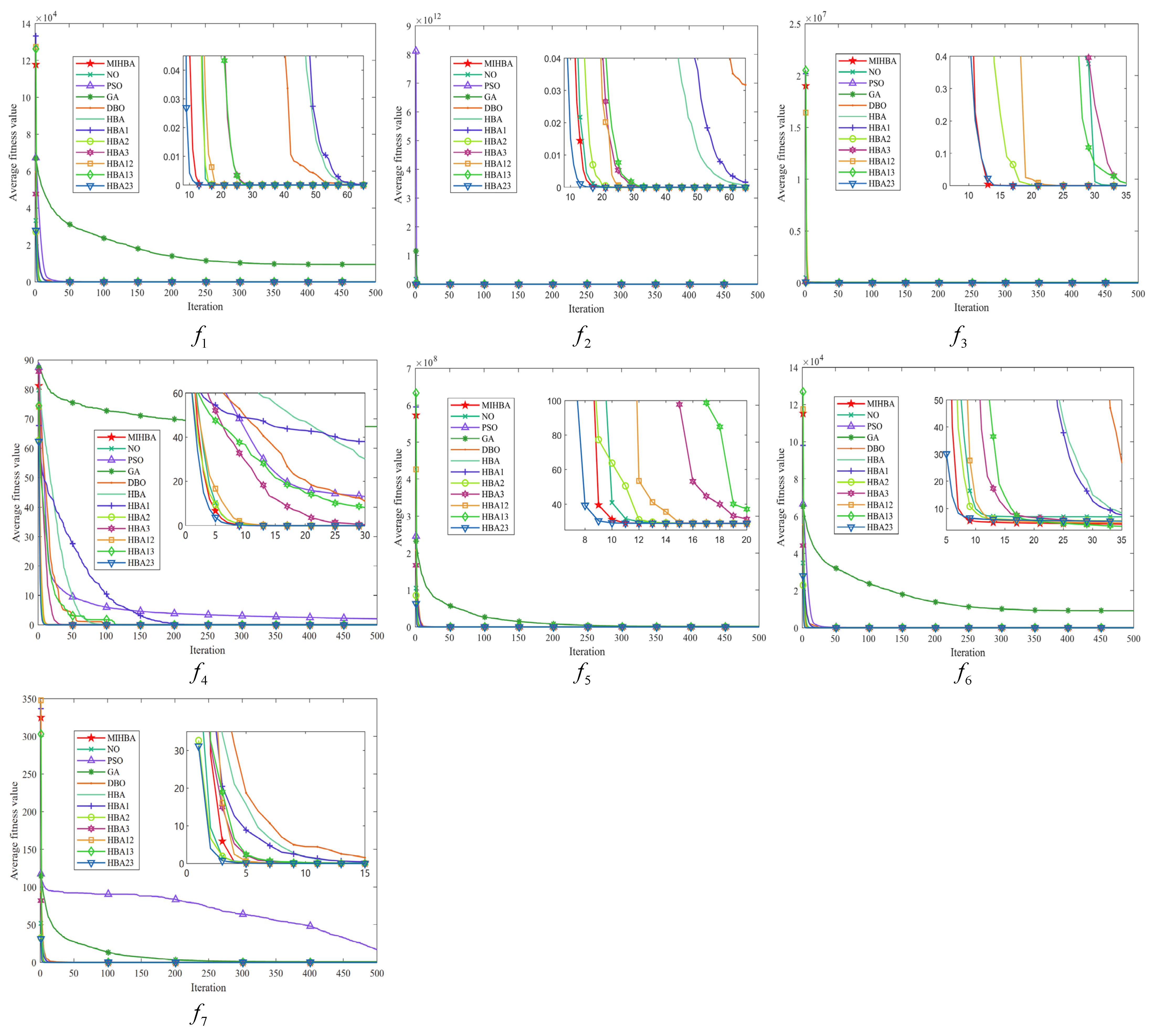
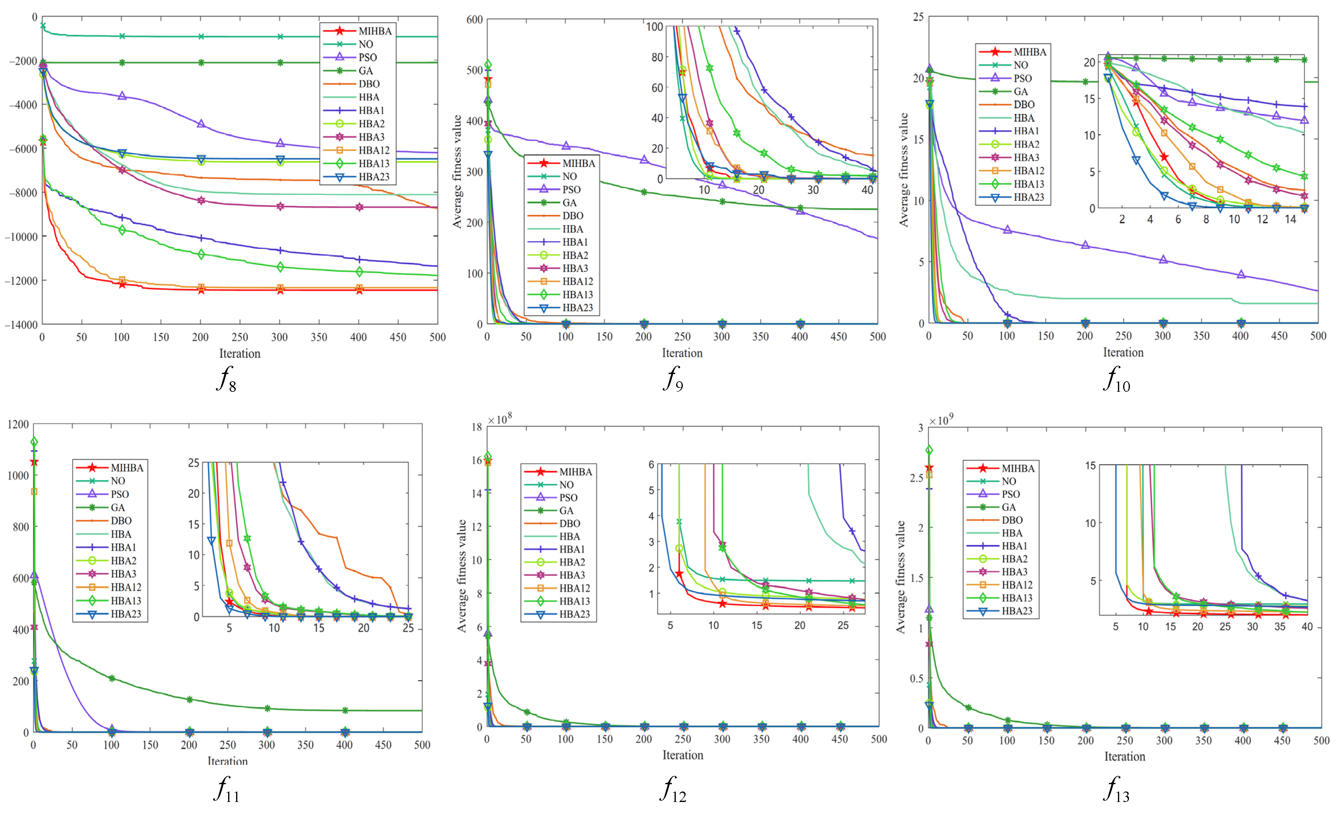
3.8. Convergence Analysis

Convergence analysis is a key metric when evaluating algorithm performance. During the iteration process, the convergence analysis can determine whether the algorithm can effectively approximate the optimal solution or reach a steady state. In this paper, we set an upper limit of 500 iterations, a population size of 30 individuals, and specify that all algorithms are evaluated for fitness no more than 15,000 times. In order to visualize the convergence behavior of the algorithms, we plotted Figure 5, Figure 6 and Figure 7, which show the average convergence curves of the MIHBA and other comparative algorithms on different types of test functions, respectively. Specifically, Figure 5 covers 7 single-peak test functions, Figure 6 contains 6 multimodal test functions, while Figure 7 shows 10 fixed-dimension test functions. These plots provide us with a visual comparison of the convergence performance of the algorithms.

Figure 5 shows the average convergence curves of the MIHBA comparison algorithms on $f_1$ to $f_7$. Except for $f_7$, both MIHBA and HBA23 algorithms are located at the bottom left of the graph, which indicates that MIHBA has a very fast convergence speed and accuracy. As for $f_7$, MIHBA is ranked 4th among the 12 compared algorithms, but it has converged to a good value in the 5th iteration, indicating that MIHBA has faster convergence speed.

Figure 6 shows the average convergence curves of MIHBA and its comparison algorithm on $f_8$–$f_{13}$, with MIHBA shown as the red line with the pentagram identifier in the figure. On the $f_9$, $f_{12}$ and $f_{13}$ test functions, MIHBA is located at the bottom of the graph. It shows that on these 3 test functions, the MIHBA is able to reach more accurate values faster. On the other three test functions, MIHBA was able to achieve a performance that ranked in the top 4 out of 12 algorithms.

Figure 7 presents the average convergence curves of the MIHBA with other comparative algorithms on the $f_{14}$– f₂₃ test functions. From the figure, it can be seen that MIHBA shows excellent results on $f_{14}$, $f_{15}$, f₁₇–$f_{19}$, $f_{21}$, and $f_{22}$ with fast convergence and high convergence accuracy. MIHBA makes up for the lack of performance of HBA23. On f₂₀, although MIHBA does not have the fastest convergence, it can be seen on the small graph that all algorithms except PSO have similar performance. Improvements to the HBA did not work well on $f_{16}$ and $f_{23}$. In summary, MIHBA has a higher convergence efficiency compared to other algorithms, indicating that the improvement of HBA is effective and enhances the convergence performance of HBA.

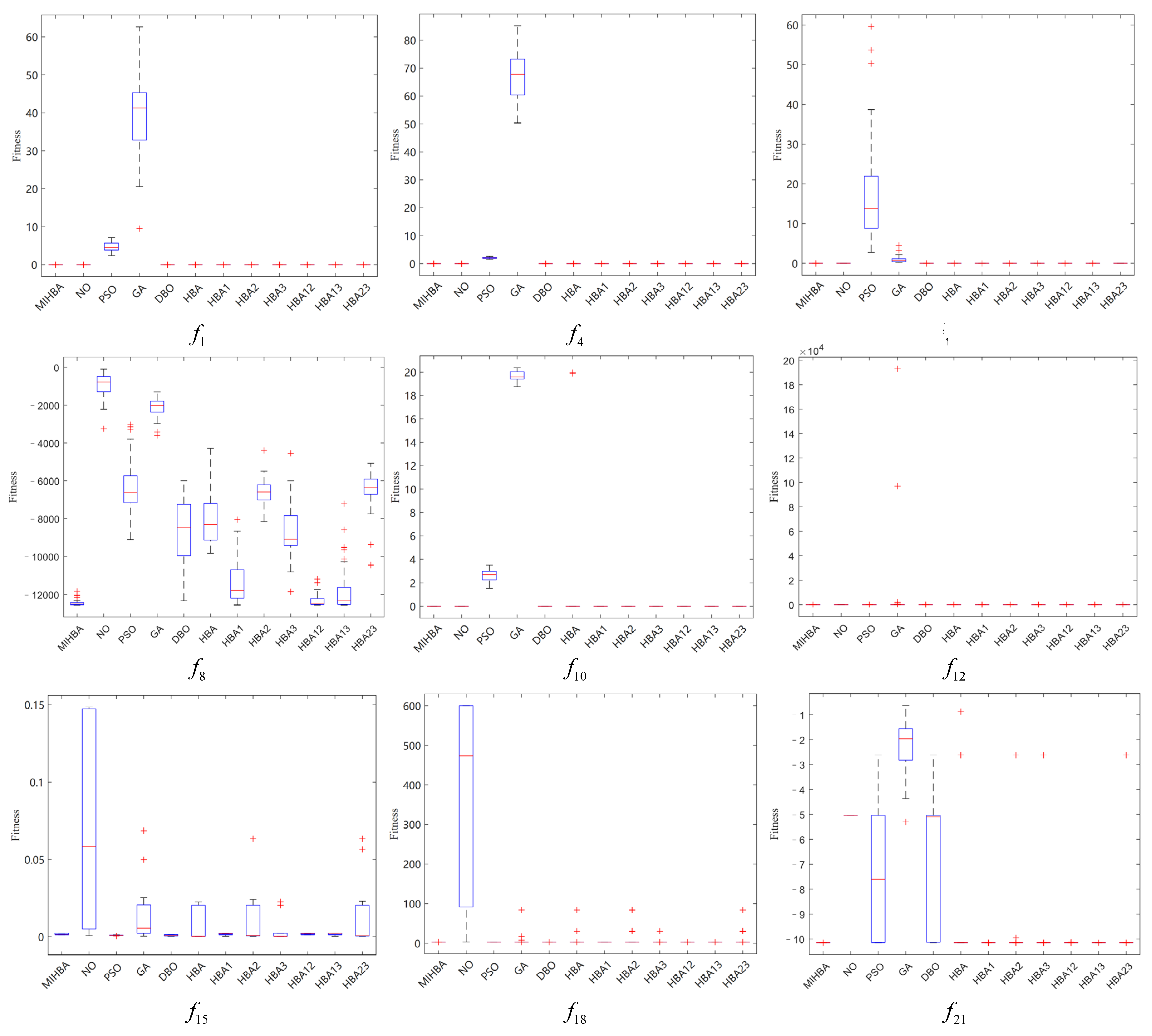
3.9. Stability Analysis

This section delves into the stability performance of the different algorithms through box plots. Each algorithm was tested with 50 independent runs. The experiments include three single-peak test functions, three multimodal test functions, and three fixed-dimension test functions for a comprehensive comparison. As shown in Figure 8, the box plot of the MIHBA is displayed side-by-side with the other compared algorithms to visually reveal the performance differences between them.

Figure 8 shows a box plot of MIHBA with the other 11 metaheuristics running 50 experiments independently. The results of the MIHBA are optimal except for $f_{12}$ and $f_{18}$, especially on $f_8$. On $f_{12}$ and f₁₈, MIHBA is stable, but there are individual outliers. MIHBA showed better stability in the experiment, suggesting that improvements to HBA are effective.

4. Application

To demonstrate the global optimization capability of the improved algorithm MIHBA, four engineering design problems are tested in this section. They are gear system design problem, pressure vessel design problem, three-bar truss design problem and reducer design problem, and the constraints are handled by applying the penalty function method. We choose the top four algorithms MIHBA, HBA, DBO and PSO ranked by Friedman test results for comparison to evaluate the performance of MIHBA. The comparison experiment is set with a population size of 30, the number of iterations is 500, and the loop experiment is conducted 50 times.

4.1. Gear Train Design Problems

A gear train consists of multiple gears that transmit motion and power, change speed, direction, and torque. Gear systems are widely used in automotive transmissions, differentials, etc. to accelerate, decelerate and steer. The design needs to consider the geometric parameters and meshing conditions to ensure that the transmission requirements are met. The transmission ratio determines the effect of deceleration or speed increase, and the design needs to consider the transmission ratio, efficiency, and cost, as shown in Figure 9. Its mathematical model is given in Equation (19).

$$\begin{array}{l}Consider\begin{array}{c}\end{array}\overrightarrow{x}=\left[x_1,x_2,x_3,x_4\right]=\left[N_1,N_2,N_3,N_4\right],\\ Minimize\begin{array}{c}\end{array}f(\overrightarrow{x})={\left({\displaystyle \frac{1}{6.931}}-{\displaystyle \frac{x_3{x}_2}{x_1{x}_4}}\right)}^2,\\ Variab\begin{array}{c}\end{array}lerange\begin{array}{c}\end{array}{x}_1,x_2,x_3,x_4\in \{12,13,\cdots ,60\}\end{array}$$

(19)

MIHBA is used to optimize the gear train design problem, and the results are compared with those of Friedman test for the top three algorithms: DBO, HBO, and PSO. As shown in the experimental results in

Table 9. Comparative experimental results for gear train design problems.

Algorithm	Optimum Value				Optimal Cost
	${\mathit{N}}_1$	${\mathit{N}}_2$	${\mathit{N}}_3$	${\mathit{N}}_4$
PSO	46	26	12	47	9.9216 × 10−10
DBO	60	12	13	18	2.7265 × 10−8
HBA	54	12	37	57	8.8876 × 10−10
MIHBA	43	19	16	49	2.7009 × 10−12

, the optimal values obtained by MIHBA are less than the other 3 algorithms, which indicates that MIHBA obtains better values and performs better in the gear train design problem. In this problem, the Optimal cost of MIHBA is reduced by two orders of magnitude compared to HBA.

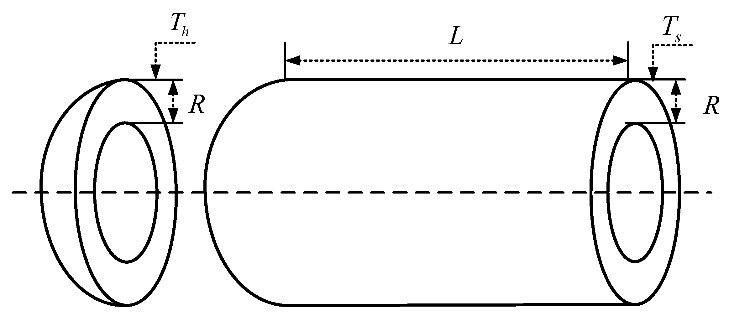
4.2. Pressure Vessel Design Problems

The pressure vessel design problem is a classical optimization problem that involves minimizing the cost of a pressure vessel while satisfying specific constraints. The mathematical model for the four parameters of this problem is given in Equation (20), and a diagram of the pressure vessel design problem is given in Figure 10.

$$\begin{array}{l}Consider\begin{array}{c}\end{array}\overrightarrow{x}=\left[x_1,x_2,x_3,x_4\right]=\left[T_s, T_h,R,L\right]\\ Minimize\begin{array}{c}\end{array}f(\overrightarrow{x})=0.6224x_1{x}_3{x}_4+1.7781x_2{x}_3^2+3.1661x_1^2{x}_4+19.84x_1^2{x}_3\\ Subject\begin{array}{c}\end{array}to\begin{array}{c}\end{array}{g}_1(\overrightarrow{x})=-x_1+0.0193x_3\le 0\\ \begin{array}{ccc}\begin{array}{cc}& \end{array}& & \end{array}\begin{array}{c}\end{array}{g}_2(\overrightarrow{x})=-x_2+0.00954x_3\le 0\\ \begin{array}{ccc}\begin{array}{cc}& \end{array}& & \end{array}\begin{array}{c}\end{array}{g}_3(\overrightarrow{x})=-\pi x_3^2{x}_4-{\displaystyle \frac{4}{3}}\pi x_3^3+1296000\le 0\\ \begin{array}{ccc}\begin{array}{cc}& \end{array}& & \end{array}\begin{array}{c}\end{array}{g}_4(\overrightarrow{x})=x_4-240\le 0\\ Variable\begin{array}{c}\end{array}range\begin{array}{c}\end{array}{x}_1,x_2\in [0,99];x_3,x_4\in [10,200]\end{array}$$

(20)

As shown in the experimental results in

Table 10. Results of comparative experiments on pressure vessel design problems.

Algorithm	Optimum Value				Optimal Cost
	${\mathit{T}}_{\mathit{s}}$	${\mathit{T}}_{\mathit{h}}$	$\mathit{R}$	$\mathit{L}$
PSO	8.8652 × 10−1	4.3823 × 10−1	4.5933 × 101	1.3428 × 102	6.0978 × 103
DBO	9.8781 × 10−1	4.8827 × 10−1	5.1182 × 101	8.9237 × 101	6.3489 × 103
HBA	1.0888 × 100	5.4029 × 10−1	5.6377 × 101	5.4621 × 101	6.6714 × 103
MIHBA	7.9079 × 10−1	3.9089 × 10−1	4.0974 × 101	1.9109 × 102	5.9073 × 103

, the optimal values obtained by MIHBA are less than the other three algorithms, indicating that MIHBA obtains better values and performs better in the pressure vessel design problems. In this problem, the Optimal cost of MIHBA is reduced by 11.45% compared to HBA.

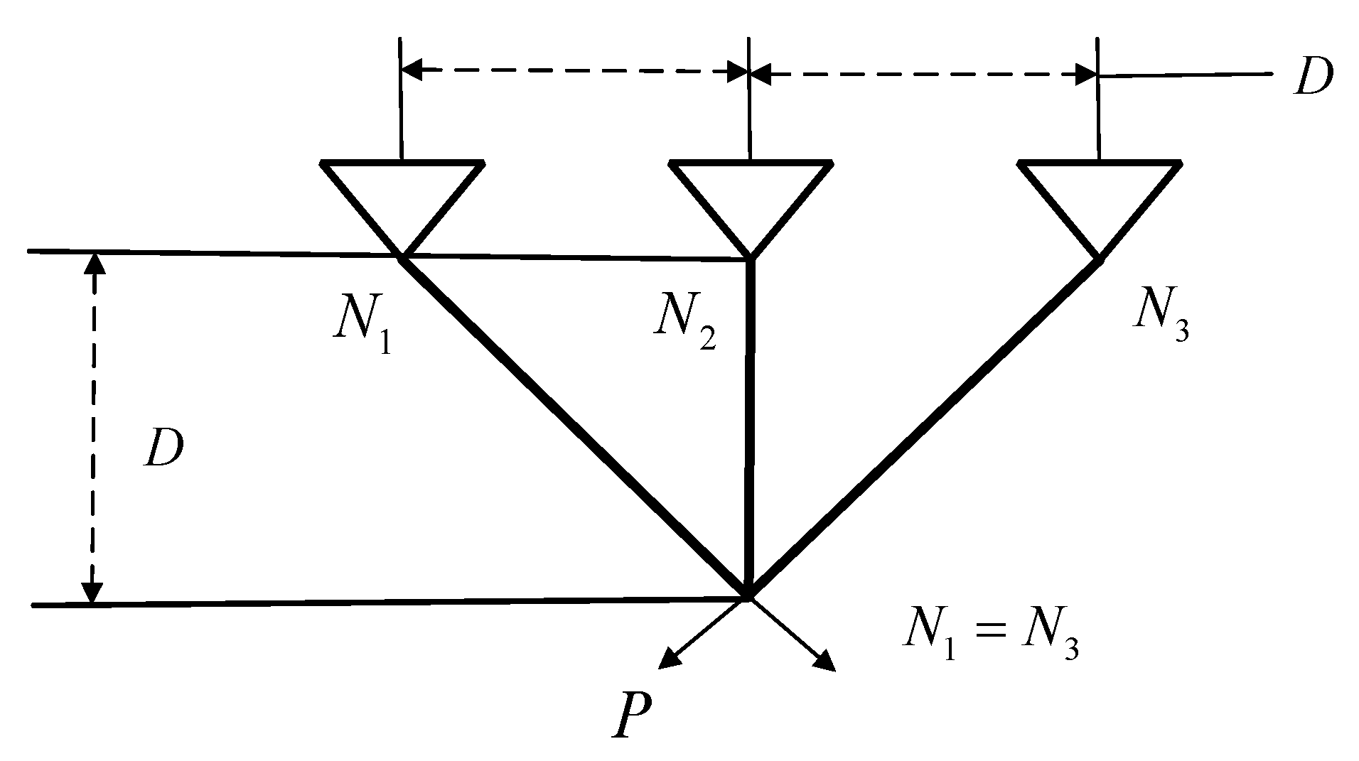
4.3. Three-Rod Truss Design Problems

The three-bar truss design problem is a classical structural optimization problem that involves mechanics and optimization theory. In this problem, the objective is to design a truss consisting of three rods that minimizes the weight of the truss under given loads and constraints while satisfying the strength, stiffness, and stability requirements, and reduces the cost of designing problems for a three-rod truss. The mathematical model for the parameters of this problem is given in Equation (21), and a diagram of the three-bar truss design problem is given in Figure 11.

$$\begin{array}{l}Consider\begin{array}{c}\end{array}\overrightarrow{x}=\left[x_1,x_2\right]=\left[N_1,N_2\right]\\ Minimize\begin{array}{c}\end{array}f(\overrightarrow{x})=L^{*}\left(2\sqrt{2}{x}_1+x_2\right)\\ Subject\begin{array}{c}\end{array}to\begin{array}{c}\end{array}{g}_1(\overrightarrow{x})={\displaystyle \frac{\sqrt{2}{x}_1+x_2}{\sqrt{2}{x}_1^2+2x_1{x}_2}}P-\delta \le 0\\ \begin{array}{cccc}& & & \end{array}\begin{array}{c}\end{array}{g}_2(\overrightarrow{x})={\displaystyle \frac{x_2}{\sqrt{2}{x}_1^2+2x_1{x}_2}}P-\delta \le 0\\ \begin{array}{cccc}& & & \end{array}\begin{array}{c}\end{array}{g}_3(\overrightarrow{x})={\displaystyle \frac{1}{\sqrt{2}{x}_2+x_1}}P-\delta \le 0\\ Variable\begin{array}{c}\end{array}range\begin{array}{c}\end{array}{x}_1,x_2\in [0,1]\\ Where\begin{array}{c}\end{array}L=100,P=2,\delta =2\end{array}$$

(21)

As shown in the experimental results in

Table 11. Comparative experimental results for the three-bar truss design problems.

Algorithm	Optimum Value		Optimal Cost
	${\mathit{N}}_1$	${\mathit{N}}_2$
PSO	7.8489 × 10−1	4.1908 × 10−1	263.9078
DBO	7.9007 × 10−1	4.0433 × 10−1	263.8983
HBA	7.9240 × 10−1	3.9780 × 10−1	263.9059
MIHBA	7.8862 × 10−1	4.0840 × 10−1	263.8958

, the optimal values obtained by MIHBA are smaller than the other three algorithms, indicating that MIHBA obtains better values and performs better in the three-bar truss design problem.

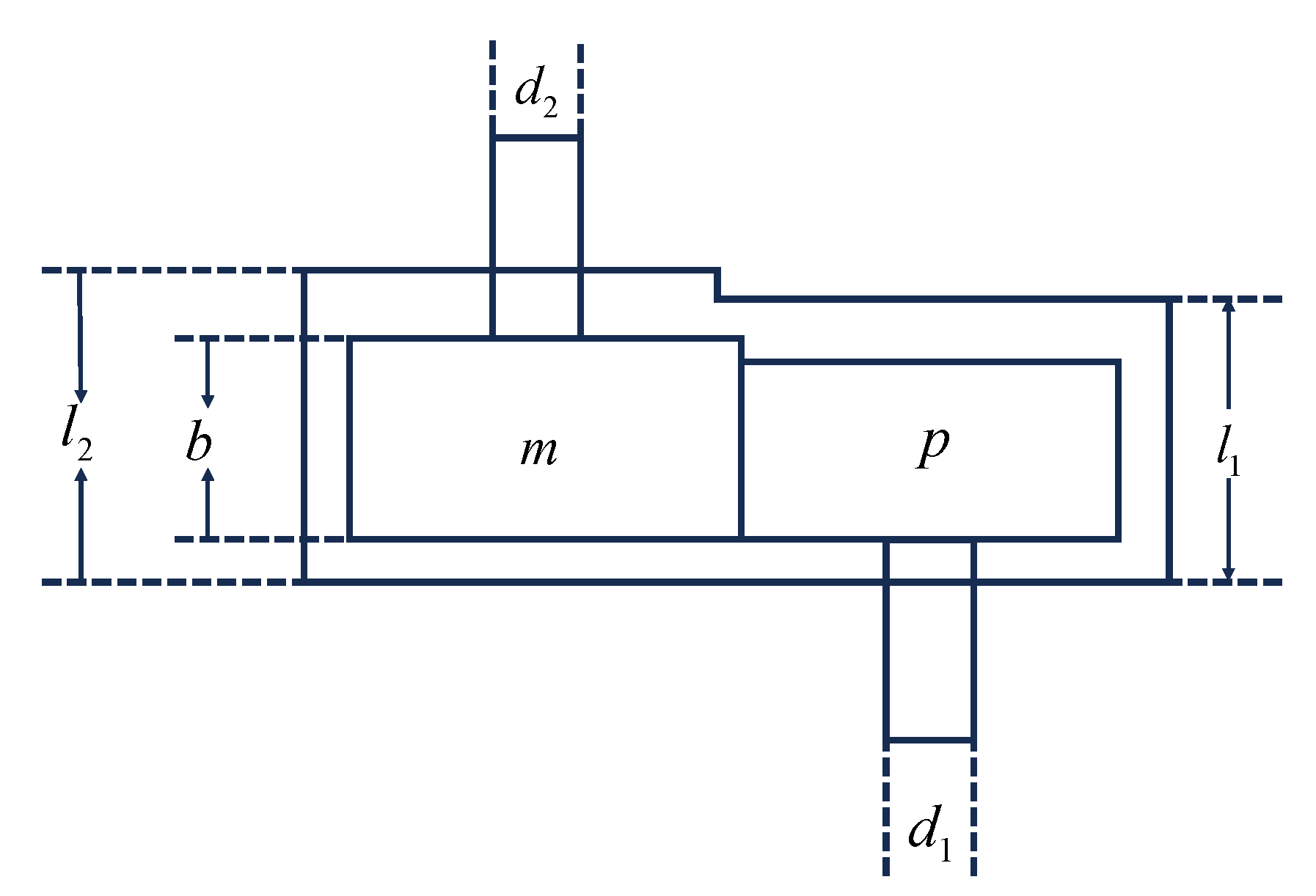
4.4. Reducer Design Problems

In the field of engineering design, the gearbox design problem is a typical optimization challenge that aims to minimize weight and design cost while satisfying a set of key performance constraints. This problem involves seven major design variables: the tooth face width $b$, the gear module $m$, the number of pinion teeth $p$, the lengths of the two shafts $l_1$ and $l_2$, and the diameters of the two shafts $d_1$ and $d_2$. Together, these variables determine the size, performance, and weight of the gearbox. To ensure the safety and reliability of the reducer, the design process must adhere to 11 stringent constraints, including bending stresses on the gear teeth, surface pressures, transverse shaft deflections, and stresses on the shaft. The gearbox design problem is shown in Figure 12, and its mathematical model is given in Equation (22).

$$\begin{array}{l}\mathit{\text{Consider}} \overrightarrow{x}=[x_1,x_2,x_3,x_4,x_5,x_6,x_7]=[b,m,p,l_1,l_2,d_1,d_2]\\ \mathit{\text{Minimize}} f(\overrightarrow{x})=0.7854x_1{x}_2^2(3.3333x_3^2+14.9334x_3-43.0934)\\ -1.508x_1(x_6^2+x_7^2)+7.4777(x_6^3+x_7^3)+0.7854(x_4{x}_6^2+x_5{x}_7^2)\\ \mathit{\text{Subject to}} g_1(\overrightarrow{x})=\frac{27}{x_1{x}_2^2{x}_3}-1\le 0\\ g_2(\overrightarrow{x})=\frac{397.5}{x_1{x}_2^2{x}_3^2}-1\le 0\\ g_3(\overrightarrow{x})=\frac{1.93x_4^3}{x_2{x}_6^4{x}_3}-1\le 0\\ g_4(\overrightarrow{x})=\frac{1.93x_5^3}{x_2{x}_7^4{x}_3}-1\le 0\\ g_5(\overrightarrow{x})=\frac{\sqrt{{\left(745x_4/\left(x_2{x}_3\right)\right)}^2+16.9\times {10}^6}}{110x_6^3}-1\le 0\\ g_6(\overrightarrow{x})=\frac{\sqrt{{\left(745x_5/\left(x_2{x}_3\right)\right)}^2+157.5\times {10}^6}}{85x_7^3}-1\le 0\\ g_7(\overrightarrow{x})=\frac{x_2{x}_3}{40}-1\le 0\\ g_8(\overrightarrow{x})=\frac{5x_2}{x_1}-1\le 0\\ g_9(\overrightarrow{x})=\frac{x_1}{12x_2}-1\le 0\\ g_{10}(\overrightarrow{x})=\frac{1.5x_6+1.9}{x_4}-1\le 0\\ g_{11}(\overrightarrow{x})=\frac{1.1x_7+1.9}{x_5}-1\le 0\\ \mathit{\text{Variable range}} x_1\in [2.6,3.6],x_2\in [0.7,0.8],x_3\in [17,28],\\ x_4\in [7.3,8.3],x_5\in [7.8,8.3],x_6\in [2.9,3.9],x_7\in [5.0,5.5]\end{array}$$

(22)

As shown in the experimental results in

Table 12. Comparative experimental results for pressure vessel design problems.

Algorithm	Optimum Value							Optimal Cost
		$\mathit{m}$		${\mathit{l}}_1$	${\mathit{l}}_2$	${\mathit{d}}_1$	${\mathit{d}}_2$
PSO	3.6	0.7	17	8.3	8.3000 × 100	3.3522 × 100	5.5000 × 100	3.1977 × 103
DBO	3.6	0.7	17	8.3	8.3000 × 100	3.3522 × 100	5.2869 × 100	3.0560 × 103
HBA	3.6	0.7	17	8.3	7.7154 × 100	3.9000 × 100	5.2867 × 100	3.2093 × 103
MIHBA	3.6	0.7	17	7.3	7.7153 × 100	3.3502 × 100	5.2867 × 100	2.9945 × 103

, the optimal values obtained by MIHBA are less than the other three algorithms, indicating that MIHBA obtains better values and performs better in the gearbox design problem. In this problem, the optimal cost of MIHBA is 6.69% lower than that of HBA.

5. Conclusions

The honey badger algorithm has important applications in the engineering field, as it can not only efficiently find the global optimal solution in complex search spaces, but also maintain a balance between exploration and exploitation, converge quickly, and be applicable to a wide range of engineering optimization problems. However, the honey badger algorithm may encounter the problems of slow convergence and easy to fall into local optimum in some cases. In this paper, the honey badger algorithm is analyzed in depth and several key improvements are proposed. These improvements include the use of Halton sequence for population initialization, the introduction of water wave dynamic density factor, and the use of a learning method based on the principles of lens imaging. These innovative strategies significantly improve the algorithm’s search power and the quality of the solution, making it more effective in dealing with complex optimization problems. Initializing the population by Halton sequence increases the diversity of the population and thus prevents the algorithm from converging to a local optimum solution too early in the search process. This approach generates a uniformly distributed set of points in the multidimensional space, providing a more balanced starting point for the global search of the algorithm. The global and local search capability of the algorithm is improved by introducing the water wave dynamic density factor to simulate the propagation, refraction, and breaking wave motion in the solution space. This dynamic density factor allows the algorithm to explore the vast search space more efficiently. In addition, a learning method based on the lens imaging principle is used to further improve the algorithm’s ability to escape from local optimal solutions. This strategy promotes communicative learning among group members by introducing new dynamics into the search process and helps to maintain the diversity of the algorithms. Finally, experiments on 23 benchmark test functions and 4 engineering design problems validate the effectiveness of the improvements. The excellent performance of MIHBA in solving complex optimization problems has been demonstrated in experiments, especially in nonlinear and multi-objective problems, which are difficult to solve using traditional mathematical methods. The advancement of MIHBA makes it a powerful tool for future work, and it has a wide range of applications spanning across many fields, such as engineering, artificial intelligence, and economic management. Whether it is model training in machine learning, structural optimization in engineering design, portfolio management in economics, or path planning in logistics, MIHBA can provide efficient solutions. Its flexibility and efficiency bode well for driving innovation and improving efficiency in the industry while closely aligning academic discoveries with industry needs. In short, MIHBAs not only has theoretical advantages, but also shows wide applicability and strong problem-solving ability in practical applications. MIHBA will play a greater role in future work to meet the needs of more industries.

Although we have made significant progress, there are still many opportunities for further improvement. The Fast Evolutionary Programming (FEP) algorithm proposed in the literature [46] can significantly improve the computational efficiency of the algorithm by parallelization strategies, especially by using modern computing resources such as GPUs, cloud computing, and other modern computing resources. Reference [47] proposes a method capable of automatically reconstructing robot models and automatically running motion simulations in a physical simulation environment by combining physical simulation modeling with Simscape Multibody and a multi-objective optimization approach with genetic algorithms in order to search for and solve the dimensions and control parameters of the robot in motion simulation. The time complexity of MIHBA proposed in this paper is not improved over that of HBA, but the time consumption is increased. In the future, we will reduce the time consumption of this algorithm and use it for solving inverse kinematics of quadrupled robots.

References

1. Xu, Y.; Cao, H.; Shi, J.; Pei, S.; Zhang, B.; She, K. A comprehensive multi-parameter optimization method of squeeze film damper-rotor system using hunter-prey optimization algorithm. Tribol. Int. 2024, 194, 109538. [Google Scholar] [CrossRef]
2. Jing, R.; Song, B.; Gao, R.; Yang, C.; Hao, X. A variable gradient descent shape optimization method for guide tee resistance reduction. J. Build. Eng. 2024, 95, 110161. [Google Scholar] [CrossRef]
3. Zhao, B.; Liu, X. A transient formulation of entropy and heat transfer coefficients of Newton’s cooling law with the unifying entropy potential difference in compressible flows. Int. J. Therm. Sci. 2024, 205, 109253. [Google Scholar] [CrossRef]
4. Lian, J.; Hui, G.; Ma, L.; Zhu, T.; Wu, X.; Heidari, A.; Chen, Y.; Chen, H. Parrot optimizer: Algorithm and applications to medical problems. Comput. Biol. Med. 2024, 172, 108064. [Google Scholar] [CrossRef] [PubMed]
5. Dehghani, M.; Montazeri, Z.; Trojovská, E. Coati Optimization Algorithm: A new bio-inspired metaheuristic algorithm for solving optimization problems. Knowl.-Based Syst. 2023, 259, 110011. [Google Scholar] [CrossRef]
6. Deng, L.; Liu, S. Snow ablation optimizer: A novel metaheuristic technique for numerical optimization and engineering design. Expert Syst. Appl. 2023, 225, 120069. [Google Scholar] [CrossRef]
7. Amiri, M.; Hashjin, N.; Montazeri, M. Hippopotamus optimization algorithm: A novel nature-inspired optimization algorithm. Sci. Rep. 2024, 14, 5032. [Google Scholar] [CrossRef]
8. Wang, J.; Wang, W.; Hu, X. Black-winged kite algorithm: A nature-inspired meta-heuristic for solving benchmark functions and engineering problems. Artif. Intell. Rev. 2024, 57, 98. [Google Scholar] [CrossRef]
9. Fan, Z.; Xiao, Z.; Li, X.; Huang, Z.; Zhang, C. MSBWO: A Multi-Strategies Improved Beluga Whale Optimization Algorithm for Feature Selection. Biomimetics 2024, 9, 572. [Google Scholar] [CrossRef] [PubMed]
10. Azizi, M.; Aickelin, U.; Khorshidi, H.A.; Baghalzadeh Shishehgarkhaneh, M. Energy valley optimizer: A novel metaheuristic algorithm for global and engineering optimization. Sci. Rep. 2023, 13, 226. [Google Scholar] [CrossRef]
11. Zolfi, K. Gold rush optimizer: A new population-based metaheuristic algorithm. Oper. Res. Decis. 2023, 33, 113–150. Available online: https://api.semanticscholar.org/CorpusID:258203735 (accessed on 16 April 2023).
12. Wang, P.; Xin, G. Quantum theory of intelligent optimization algorithms. Acta Autom. Sin. 2023, 49, 2396–2408. [Google Scholar] [CrossRef]
13. Trojovská, E.; Dehghani, M.; Trojovský, P. Zebra Optimization Algorithm: A New Bio-Inspired Optimization Algorithm for Solving Optimization Algorithm. IEEE Access 2022, 10, 49445–49473. [Google Scholar] [CrossRef]
14. Abdel-Basset, M.; Mohamed, R.; Jameel, M.; Abouhawwash, M. Nutcracker optimizer: A novel nature-inspired metaheuristic algorithm for global optimization and engineering design problems. Knowl.-Based Syst. 2022, 262, 110248. [Google Scholar] [CrossRef]
15. Abualigah, L.; Elaziz, M.; Sumari, P.; Geem, Z.; Gandomi, A. Reptile Search Algorithm (RSA): A nature-inspired meta-heuristic optimizer. Expert Syst. Appl. 2022, 191, 116158. [Google Scholar] [CrossRef]
16. Dehkordi, A.; Sadiq, A.; Mirjalili, S.; Ghafoor, K. Nonlinear-based Chaotic Harris Hawks Optimizer: Algorithm and Internet of Vehicles application. Appl. Soft Comput. 2021, 109, 107574. [Google Scholar] [CrossRef]
17. Jena, B.; Naik, M.K.; Wunnava, A.; Panda, R. A Differential Squirrel Search Algorithm. Adv. Intell. Comput. Commun. 2021, 202, 143–152. [Google Scholar] [CrossRef]
18. Faramarzi, A.; Heidarinejad, M.; Stephens, B.; Mirjalili, S. Equilibrium optimizer: A novel optimization algorithm. Knowl.-Based Syst. 2020, 191, 105190. [Google Scholar] [CrossRef]
19. Zhao, W.; Zhang, Z.; Wang, L. Manta ray foraging optimization: An effective bio-inspired optimizer for engineering applications. Eng. Appl. Artif. Intell. 2020, 87, 103300. [Google Scholar] [CrossRef]
20. Liu, Z.; Nishi, T. Multipopulation Ensemble Particle Swarm Optimizer for Engineering Design Problems. Math. Probl. Eng. 2020, 2020, 1450985. [Google Scholar] [CrossRef]
21. Hashim, F.; Houssein, E.; Hussain, K.; Mabrouk, M.; Al-Atabany, W. Honey Badger Algorithm: New metaheuristic algorithm for solving optimization problems. Math. Comput. Simul. 2022, 192, 84–110. [Google Scholar] [CrossRef]
22. Bansal, A.; Sangtani, V.; Bhukya, M. Optimal configuration and sensitivity analysis of hybrid nanogrid for futuristic residential application using honey badger algorithm. Energy Convers. Manag. 2024, 315, 118784. [Google Scholar] [CrossRef]
23. Jose, R.; Paulraj, E.; Rajesh, P. Enhancing Steady-State power flow optimization in smart grids with a hybrid converter using GBDT-HBA technique. Expert Syst. Appl. 2024, 258, 125047. [Google Scholar] [CrossRef]
24. Wilson, A.; Kiran, W.; Radhamani, A.; Bharathi, A. Optimizing energy-efficient cluster head selection in wireless sensor networks using a binarized spiking neural network and honey badger algorithm. Knowl.-Based Syst. 2024, 299, 112039. [Google Scholar] [CrossRef]
25. Jiang, M.; Ding, K.; Chen, X.; Cui, L.; Zhang, J.; Cang, Y. Cgh-gto method for model parameter identification based on improved grey wolf optimizer, honey badger algorithm, and gorilla troops optimizer. Energy 2024, 296, 131163. [Google Scholar] [CrossRef]
26. Ren, X.; Li, L.; Ji, B.; Liu, J. Design and analysis of solar hybrid combined cooling, heating and power system: A bi-level optimization model. Energy 2024, 292, 130362. [Google Scholar] [CrossRef]
27. Wang, B.; Kang, H.; Sun, G.; Li, J. Efficient traffic-based IoT device identification using a feature selection approach with Lévy flight-based sine chaotic sub-swarm binary honey badger algorithm. Appl. Soft Comput. 2024, 155, 111455. [Google Scholar] [CrossRef]
28. Zhang, S.; Wang, J.; Li, Y.; Zhang, S.; Wang, Y.; Wang, X. Improved honey badger algorithm based on elementary function density factors and mathematical spirals in polar coor-dinate systema. Artif. Intell. Rev. 2024, 57, 55. [Google Scholar] [CrossRef]
29. Huang, P.; Zhou, Y.; Deng, W.; Zhao, H.; Luo, Q.; Wei, Y. Orthogonal opposition-based learning honey badger algorithm with differential evolution for global optimization and engineering design problems. Alex. Eng. J. 2024, 91, 348–367. [Google Scholar] [CrossRef]
30. Zhang, J.; Zhang, T.; Li, C. Migration time prediction and assessment of toxic fumes under forced ventilation in underground mines. Undergr. Space 2024, 18, 273–294. [Google Scholar] [CrossRef]
31. Zhong, H.; Cong, M.; Wang, M.; Du, Y.; Liu, D. HB-RRT: A path planning algorithm for mobile robots using Halton sequence-based rapidly-exploring random tree. Eng. Appl. Artif. Intell. 2024, 133, 108362. [Google Scholar] [CrossRef]
32. Duan, Y.; Yu, X. A collaboration-based hybrid GWO-SCA optimizer for engineering optimization problems. Eng. Appl. Artif. Intell. 2023, 2013, 119017. [Google Scholar] [CrossRef]
33. Huang, Y.; Liu, Q.; Song, H.; Han, T.; Li, T. CMGWO: Grey wolf optimizer for fusion cell-like P systems. Heliyon 2024, 10, e34496. [Google Scholar] [CrossRef] [PubMed]
34. Zheng, Y. Water wave optimization: A new nature-inspired metaheuristic. Comput. Oper. Res. 2015, 55, 1–11. [Google Scholar] [CrossRef]
35. Yu, F.; Guan, J.; Wu, H.; Chen, Y.; Xia, X. Lens imaging opposition-based learning for differential evolution with cauchy perturbation. Appl. Soft Comput. 2024, 152, 111211. [Google Scholar] [CrossRef]
36. Choi, T.; Pachauri, N. Adaptive search space for stochastic opposition-based learning in differential evolution. Knowl.-Based Syst. 2024, 300, 112172. [Google Scholar] [CrossRef]
37. Bernardo, M.; Daniel, Z.; Erik, C.; Fernando, F.; Alma, R. A better balance in me-taheuristic algorithms: Does it exist? Swarm. Evol. Comput. 2020, 54, 100671. [Google Scholar] [CrossRef]
38. Abdi, G.; Sheikhani, A.; Kordrostami, S.; Zarei, B.; Rad, M. Identifying communities in complex networks using learning-based genetic algorithm. Ain Shams Eng. J. 2024, in press. [Google Scholar] [CrossRef]
39. Lyu, Y.; Jin, X.; Xue, Q.; Jia, Z.; Du, Z. An optimal configuration strategy of multi-chiller system based on overlap analysis and improved GA. Build. Environ. 2024, 266, 112117. [Google Scholar] [CrossRef]
40. Abualigah, L.; Al-qaness, M.; Abd, E. The non-monopolize search (NO): A novel single-based local search optimization algorithm. Neural Comput. Appl. 2024, 36, 5305–5332. [Google Scholar] [CrossRef]
41. Zhu, D.; Shen, J.; Zhang, Y.; Li, W.; Zhu, X.; Zhou, C.; Cheng, S.; Yao, Y. Multi-strategy particle swarm optimization with adaptive forgetting for base station layout. Swarm Evol. Comput. 2024, 91, 101737. [Google Scholar] [CrossRef]
42. Hu, Q.; Zhou, N.; Chen, H.; Weng, S. Bayesian damage identification of an unsymmetrical frame structure with an improved PSO algorithm. Structures 2023, 57, 105119. [Google Scholar] [CrossRef]
43. Lu, Q.; Chen, Y.; Zhang, X. Grinding process optimization considering carbon emissions, cost and time based on an improved dung beetle algorithm. Comput. Ind. Eng. 2024, 197, 110600. [Google Scholar] [CrossRef]
44. Röhmel, J. The permutation distribution of the Friedman test. Comput. Stat. Data Anal. 1997, 26, 83–99. [Google Scholar] [CrossRef]
45. Dewan, I.; Rao, B. Wilcoxon-signed rank test for associated sequences. Stat. Probab. Lett. 2005, 71, 131–142. [Google Scholar] [CrossRef]
46. Zhuo, Y.; Zhang, T.; Du, F.; Liu, R. A parallel particle swarm optimization algorithm based on GPU/CUDA. Appl. Soft Comput. 2023, 144, 110499. [Google Scholar] [CrossRef]
47. Xiao, Y.; Yin, K.; Chen, X.; Chen, Z.; Gao, F. Multi-objective optimization design method for the dimensions and control parameters of curling hexapod robot based on application performance. Mech. Mach. Theory 2024, 204, 105831. [Google Scholar] [CrossRef]
Figure 1. Population initialization. (a) Random distribution map, (b) Halton distribution map, (c) Random initialized particle swarm distribution histogram, (d) Halton initialized particle swarm distribution histogram.
Algorithms 17 00573 g001
Figure 2. Four different convergence factors. (a) The original convergence factor shown in Equation (3), (b) the sinusoidal convergence factor shown in Equation (10), (c) the power-of-five convergence factor demonstrated in Equation (11), and (d) the water wave dynamic density factor shown in Equation (12).
Algorithms 17 00573 g002
Figure 3. LOBL schematic.
Algorithms 17 00573 g003
Figure 4. Overall flowchart of the improved algorithm.
Algorithms 17 00573 g004
Figure 5. Average convergence curves of MIHBA and comparative algorithms on single-peak test functions.
Algorithms 17 00573 g005
Figure 6. Average convergence curves of MIHBA and comparison algorithm on multimodal test functions.
Algorithms 17 00573 g006
Figure 7. Average convergence curves of MIHBA and comparison algorithms on fixed dimensional test functions.
Algorithms 17 00573 g007
Figure 8. Box-line diagram of MIHBA and comparison algorithms.
Algorithms 17 00573 g008
Figure 9. Diagram of gear system design problems.
Algorithms 17 00573 g009
Figure 10. Pressure vessel design problem map.
Algorithms 17 00573 g010
Figure 11. Problematic diagram of three-rod truss design.
Algorithms 17 00573 g011
Figure 12. Schemes follow the same formatting.
Algorithms 17 00573 g012