Search on an NK Landscape with Swarm Intelligence: Limitations and Future Research Opportunities

Abstract

Swarm intelligence has promising applications for firm search and decision-choice problems and is particularly well suited for examining how other firms influence the focal firm’s search. To evaluate search performance, researchers examining firm search through simulation models typically build a performance landscape. The NK model is the leading tool used for this purpose in the management science literature. We assess the usefulness of the NK landscape for simulated swarm search. We find that the strength of the swarm model for examining firm search and decision-choice problems—the ability to model the influence of other firms on the focal firm—is limited to the NK landscape. Researchers will need alternative ways to create a performance landscape in order to use our full swarm model in simulations. We also identify multiple opportunities—endogenous landscapes, agent-specific landscapes, incomplete information, and costly movements—that future researchers can include in landscape development to gain the maximum insights from swarm-based firm search simulations.

1. Introduction

Firm managers are often faced with complex problems that require searching across many, potentially interdependent elements in order to make a choice with significant financial consequences [1]. Examples include developing new products, designing organizational processes, or assembling resources. To examine these problems, strategic management and organizational science scholars often employ simulations of search strategies [2]. To evaluate strategy performance, scholars typically apply the search strategy to a performance or fitness landscape. The leading tool for this, the NK model, has been highly influential in the strategy and management science literature and has been applied to a variety of search problems [3]. Using NK, the researcher can create a performance landscape consisting of N components with K interdependencies. As K increases, the landscape becomes more rugged, with more peaks and valleys [4].

Recently, scholars interested in how competitors influence firm search have turned to swarm intelligence models [5]. Unlike previous firm search models that focused only on the firm’s own performance feedback, swarm models allow for the various behaviors of other firms to influence the focal firm’s search strategy. For instance, Chen, Miller, and Toh (2023) develop a swarm intelligence model that provides a flexible way to incorporate a range of competitive influences, and they demonstrate how to use patent filings and patent citation data to fit the model parameters and assess search performance [5]. However, to investigate many problems, scholars will want to develop simulations to enable them to abstract from the constraints of real-world data. Swarm simulations appear to have many promising applications for firm search and choice problems, but to utilize simulations effectively, the researcher needs to devise a performance landscape in order to evaluate the effectiveness of different search strategies. The best way to form a search landscape for swarm remains unclear. A natural place to start is to simulate swarm search on the current leading landscape tool—NK.

In this paper, we assess whether NK provides a suitable performance landscape to conduct realistic swarm-based simulations of firm behavior. Note that our focus is not on evaluating the effectiveness of our swarm algorithm on the NK landscape, as one might evaluate the effectiveness of different optimization models to solve a particular problem; rather, we want to know if the swarm-NK combination allows one to study firm search phenomena in a realistic and insightful manner. We apply the Boids-based algorithm of Chen et al. [5] to various NK landscapes. We find that because search on an NK landscape is limited to movements along the hypercube rather than continuous movements in real space, we cannot harness the full power of our swarm model. In fact, we can only have one variable influence search at a time, thus collapsing our multivariate model into a simple univariate model. Therefore, using NK to generate the performance landscape constrains our swarm model from incorporating a full range of information from the environment. A different way to generate the performance landscape is needed to harness the full potential of our swarm model.

Through our investigation, we also uncover a variety of potential technical needs that could allow strategy and organizational scholars to apply swarm models in a richer way. Our main contribution is identifying necessary features (such as more appropriate landscape attributes) to improve swarm search. We hope that by identifying these gaps, researchers, including those in computer science and adjacent fields, can contribute to the development of swarm search and its application to firm search and decision-choice problems. We briefly summarize the potential research directions below.

Future Research Directions

• A payoff landscape or function that allows for continuous movement so that the full value of swarm in modeling agent (firm or human) behavior can be realized.
• Endogenous landscapes that allow payoffs to change as a function of agents positions on the landscape.
• Agent-specific landscapes that allow for researchers to explore heterogeneous returns to agent actions.
• Allowing information between agents, their locations, and their performance to be uncertain or incomplete.
• Including the cost of movements into the framework rather than implicitly assuming free movements on the landscape.

The paper is structured as follows: Section 2 briefly discusses the NK landscape. Section 3 describes the swarm model. Section 4 describes search algorithms for NK landscapes. Section 5 displays the swarm simulation results. Section 6 discusses the limitations of NK landscapes for swarms. Section 7 lays out future research directions. Section 8 concludes the article.

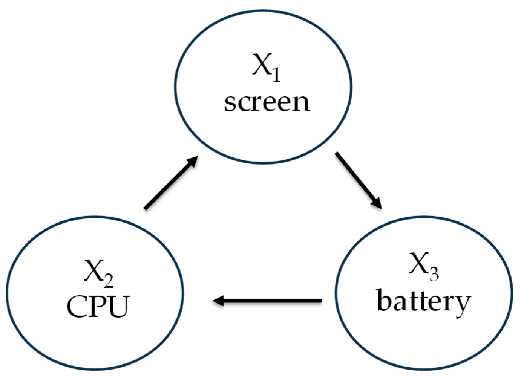
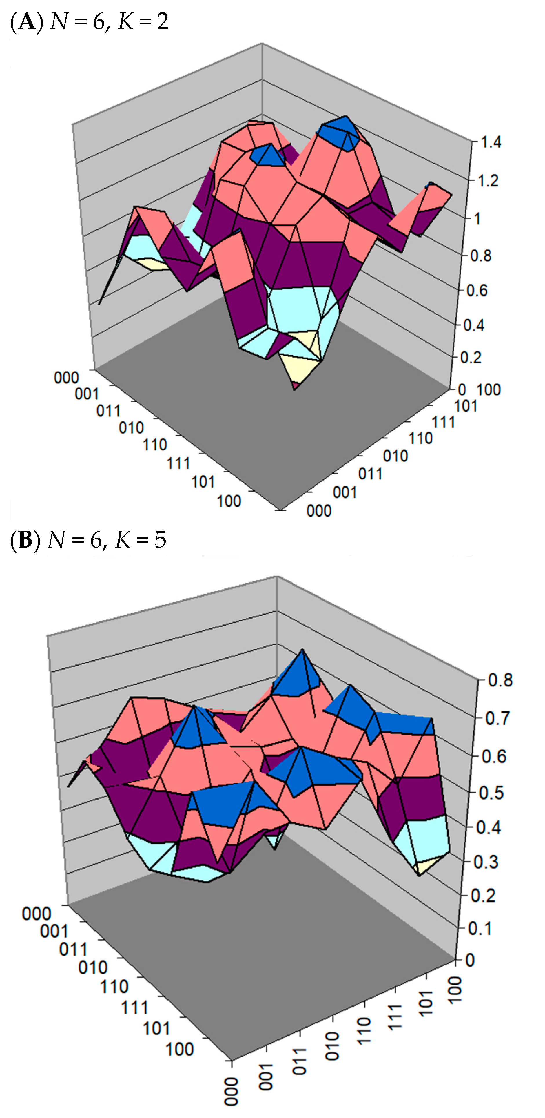
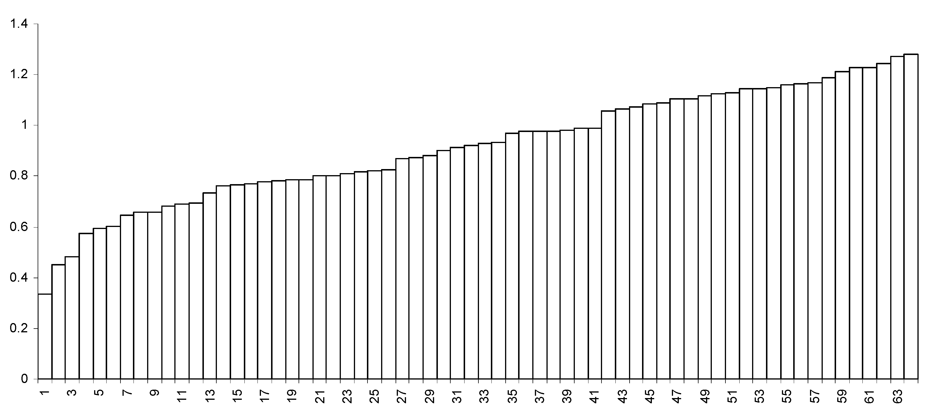
2. NK Landscape

2.1. Background

The NK landscape model is a computational tool used for studying complex systems. Introduced by Stuart Kauffman in the late 1980s to study biological systems [6,7], NK has since found applications in various disciplines, including strategic management, economics, and organizational studies, to examine firm choice [8].

In an NK landscape model, a system consists of N components, each of which can exist in a certain state. Each component’s state is influenced by K other components. The total possible states for a system are 2^N. Each combination of component states has a ‘fitness’ associated with it, which is a measure of how well the system is performing in that particular state. Depending on the interactions among components, the fitness or performance landscape can be visualized as a surface with peaks (high fitness) and valleys (low fitness). A smooth landscape has fewer local optima, while a rugged landscape has many.

In a rugged landscape, finding the global optimum is challenging [9]. Firms must strike a balance between exploiting known solutions (climbing the local peak) and exploring new potential solutions (searching elsewhere in the landscape). As K (interdependencies) increases, the landscape becomes more rugged. Rugged landscapes represent highly interdependent environments, which deteriorates the performance of local search. On rugged landscapes, agents need to adopt more flexible and adaptive search strategies.

While being a powerful tool, the NK model has limitations. First, it reduces the complex interactions of real-world systems into binary choices, which we will show later, which constrains their potential to be combined with swarm intelligence models. Second, the model assumes that interactions between components are randomly distributed and remain constant, which might not be the case in real-world scenarios. Third, setting appropriate N and K values to accurately represent a real-world system can be challenging. Ganco and Hoetker (2009) provide a nice review of the NK landscape used in the strategy literature and details of the NK landscape implementation [3].

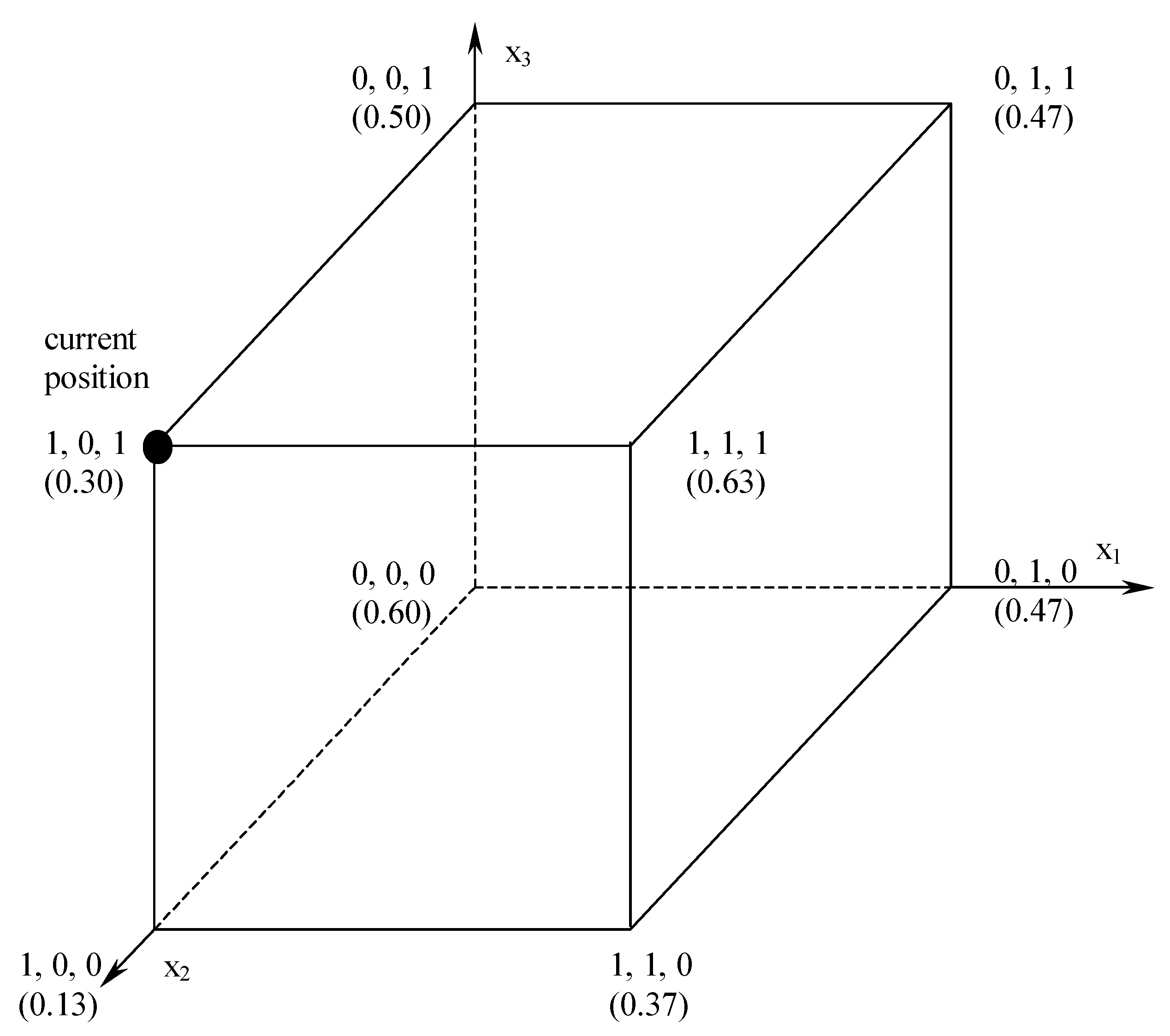
2.2. Mathematical Development of NK

In the strategy and organization literature, an NK landscape is usually described by a set of binary choices. As a result, the landscape is a high-dimensional hypercube. Csaszar (2018) gives an example of three major components of a computer: the screen, CPU, and battery. These three components are interdependent. His diagram is reproduced here in Figure 1.

In Figure 1, the arrows represent the direction of influence. The battery depends on the screen, the CPU depends on the battery, and the screen depends on the CPU. These interdependencies are usually described by an interaction matrix (IM). Figure 1 can be written formally as follows:

$$I=\begin{array}{cc}& \begin{array}{}{x}_1{x}_2{x}_3\end{array}\\ \begin{array}{c}{x}_1\\ x_2\\ x_3\end{array}& \left[\begin{array}{ccc}1& 0& 1\\ 1& 1& 0\\ 0& 1& 1\end{array}\right]\end{array}$$

(1)

In which the direction of influence goes from top to left. In other words, each row describes how a component is influenced by the other components. In other words, $x_1$ (first row) is influenced by itself and $x_3$, $x_2$ (second row) is influenced by itself and $x_1$, and $x_3$ (third row) is influenced by itself and $x_2$.

The NK landscape model is usually described as an N-dimensional hypercube with binary (0/1) values at each node. We can visualize an N = 3 hypercube as shown in Figure 2. Each node, from $[0,0,0]$ to $[1,1,1]$, represents each component’s state. In this binary setting, there are only two states (e.g., on or off).

If we examine $x_1$ (screen), since we know it is influenced by only $x_3$ (CPU), we should have the following information for fitness ${\varphi }_1(x_1,x_3)$. Similarly, we have ${\varphi }_2(x_2,x_1)$ and ${\varphi }_3(x_3,x_2)$. Simply speaking, each sub-fitness function ${\varphi }_i$ is evaluated for all components that influence component i. We write it out explicitly as follows:

$${\varphi }_1(x_1,x_3)=\left\{\begin{array}{l}{\varphi }_1(0,0)\\ {\varphi }_1(0,1)\\ {\varphi }_1(1,0)\\ {\varphi }_1(1,1)\end{array}\right.\hspace{1em}{\varphi }_2(x_2,x_1)=\left\{\begin{array}{l}{\varphi }_2(0,0)\\ {\varphi }_2(0,1)\\ {\varphi }_2(1,0)\\ {\varphi }_2(1,1)\end{array}\right.\hspace{1em}{\varphi }_3(x_3,x_2)=\left\{\begin{array}{l}{\varphi }_3(0,0)\\ {\varphi }_3(0,1)\\ {\varphi }_3(1,0)\\ {\varphi }_3(1,1)\end{array}\right.$$

(2)

$$\varphi (x_1,x_2,x_3)={\varphi }_1(x_1,x_3)+{\varphi }_2(x_2,x_1)+{\varphi }_3(x_3,x_2)$$

(3)

For example,

$$\varphi (1,0,1)={\varphi }_1(1,1)+{\varphi }_2(0,1)+{\varphi }_3(1,0)$$

(4)

The entire landscape is the hypercube, which includes all the possible points, as demonstrated in Figure 2. The fitness values are presented in parentheses (the global peak is 0.6333 at 1, 1, 1). The major drawback of Figure 2 is that the landscape it represents cannot be visualized.

In a general sense, the fitness function of any choice of policy can be written as:

$$\varphi (x_1,\cdots ,x_N)=\frac{1}{N}{\displaystyle {\sum }_{i=1}^N}{\varphi }_i(x_i\in I_i)$$

(5)

where $x_i=0,1$ and $I_i$ represents the ith row of the interaction matrix I.

Once the number of components is greater than 3, it is not possible to graphically draw the hypercube. Furthermore, the hypercube cannot present a visual of the landscape. As a result, it is common in the NK landscape literature to collapse the N-dimensional hypercube into a three-dimensional landscape, which can then be visualized, as in Figure 3 [10]. However, the usual description of a 3-D collapsed landscape often seen in the literature is not an actual collapse of the hypercube but rather an imaginary portrait to mimic the ruggedness of the landscape [11]. As seen in Figure 3, high K results in a rugged landscape, while low K results in a smooth landscape.

In this paper, we first follow Ganco and Hoetker [3] and use $N=6$ to demonstrate our swarm simulations. We set up two cases: K = 2 to represent a few interdependencies, and K = 5 to represent the maximum interdependencies.

For example, when $N=6$, then there are $2^6=64$ choices from $[0,0,0,0,0,0]$ to $[1,1,1,1,1,1]$ (or 0–63 in decimal representation). Hence, there are 64 fitness values, one for each choice. In other words, this is a six-dimensional hypercube. Each sub-fitness function ${\varphi }_i$ is used as in Equation (5).

3. Swarm Intelligence Algorithms

3.1. Background

Swarm intelligence is the collective behavior of a decentralized system [12]. The motivation for swarm intelligence comes from animals, such as birds, ants, bees, and fish, that rely on group effort to achieve their basic survival needs, like seeking food or avoiding prey [13]. Swarm intelligence has been used to study the behaviors of biological organisms, tackle technical problems in engineering and medicine, and solve optimization problems [14]. In this subsection, we briefly review the literature that applies swarm to optimization and technical problems before turning to our main focus in Section 3.2—using the Boids [15] version of swarm to study agent search behavior. Perhaps the most active area of swarm-related research is its application to solve optimization problems [14]. Eberhart and Kennedy (1995) were the first to adapt the behavioral model of swarm into an objective-seeking algorithm known as particle swarm optimization (PSO) [16]. Their model “artificializes” the group behavior of a flock of birds seeking food. Via bird-to-bird chirping (i.e., peer-to-peer communication), all birds fly to the loudest sound of chirping. Shi and Eberhart (1998) improve the model by adding an inertia term to seek a balance between exploitation and exploration [17]. Since then, researchers have applied PSO to a variety of contexts. For instance, PSO has been used for efficient frontier estimation [18], portfolio optimization [19,20,21,22,23,24], interest rate modeling [25], earnings forecasting [26], and inventory management [27].

A search on an NK landscape is composed of making multiple binary decisions. Researchers have modified the PSO algorithm to operate on binary problems [28] like modeling genes. For example, Lee et al. (2008) and Di Caro (2019) introduce a modified binary PSO in which binary and continuous positions can be connected via a response/sigmoid function like in the logit model [29,30]. Later work developed a momentum search algorithm to enhance how PSO searches [31]. Recent research examines how to alter velocity, momentum, exploration, and exploitation to make binary PSO more effective and efficient [32]. In this paper, for our purposes, we use a fixed value cutoff as opposed to the response/sigmoid function as in Lee et al. (2008).

Swarm optimization models have also been applied in conjunction with other methods to solve a variety of problems. For instance, swarm intelligence has been applied to tune hyperparameters in ensemble deep learning models [33], enhance neural networks [34,35], and supplement other deep learning approaches [36]. The relative performance of different swarm intelligence algorithms is not always understood; however, there is burgeoning work in this area. For instance, Guerra et al. (2023) compare how four swarm algorithms perform in optimizing unscented Kalman filter parameters in a robotics application [37]. We refer those interested in algorithm performance comparisons in technical applications or dimension reduction to the following work [38,39,40,41].

3.2. Swarm Intelligence to Model Agent Behavior

Swarm intelligence can be used to analyze human behavior. For instance, swarm intelligence has been used to examine blog posts to understand human collective behavior [42]. It has also been proposed as a tool to understand the dynamic casual mechanisms that underlie human team outcomes [43]. Minar et al. (1996) created an agent-based simulations software for performing multiagent simulations [44]. Coen and Maritan (2011) use Minar et al.’s software to develop an agent-based model of resource allocation, exploring how the firm’s search ability and initial capability endowment influence performance in a competitive environment [45].

In this paper, we simulate firm search on a performance landscape. Our departure point is Chen et al. [5], who apply swarm intelligence to examine how firms search for new technological inventions. They fit an augmented version of Reynold’s model to patent data to assess if a firm’s search is influenced by other firms or by its own past performance. Since our goal is to simulate the Reynold’s Boids model on an NK landscape, we briefly discuss this model before proceeding to the mathematical development.

Reynold (1987) [15] was the first to “artificialize” natural intelligence by creating the Boids (or bird-oid object) computer algorithm. For any given bird, Reynold devises a set of linear equations (vectors) that combine to determine how the bird should fly to its next destination. The equations contain three factors: separation, alignment, and cohesion. As their names suggest, “separation” is to avoid collision with other birds, “alignment” controls how a particular bird should fly in a direction by referencing its fellow birds, and “cohesion” decides how fast a particular bird should fly to its next target position. Reynold’s swarm model is extremely easy to implement. There are countless versions of Boids, some of which add obstacles, objective destinations, or mazes. We now turn to the mathematical development of our swarm model.

3.3. Mathematical Development of Swarm

In a swarm, let $i$ be firm (fish) $i=1\cdots m$, t be the time, and $j$ be a corporate function $j=1\cdots n$. Let ${\stackrel{\rightharpoonup }{x}}_t^{(i)}$ represent the position of the set of choices of the ith firm at time $t$ and $x_{j,t}^{(i)}$ be the jth element. For the sake of completeness, define $F$ as the set of firms $F=\{f^{(1)},\cdots ,f^{(m)}\}$ whose positions at time $t$ we define by the $n\times m$ matrix $X_t=\{{\stackrel{\rightharpoonup }{x}}_t^{(1)},\cdots ,{\stackrel{\rightharpoonup }{x}}_t^{(m)}\}$.

The velocity of a firm is defined as follows:

$${\stackrel{\rightharpoonup }{v}}_t^{(i)}=w_A{\stackrel{\rightharpoonup }{v}}_{A,t}^{(i)}+w_C{\stackrel{\rightharpoonup }{v}}_{C,t}^{(i)}+w_L{\stackrel{\rightharpoonup }{v}}_{L,t}^{(i)}+w_S{\stackrel{\rightharpoonup }{v}}_{S,t}^{(i)}+w_P{\stackrel{\rightharpoonup }{v}}_{P,t}^{(i)}$$

(6)

where each element in vector ${\stackrel{\rightharpoonup }{v}}_t^{(i)}$ is $v_{j,t}^{(i)}$ with $i=1\cdots m$ and $j=1\cdots n$ and ${\Sigma }_{x=A}^P{w}_x=1$. Each sub-velocity is defined as follows:

$$\begin{array}{l}{\stackrel{\rightharpoonup }{v}}_{A,t}^{(i)}=\mathrm{avg}\left({\stackrel{\rightharpoonup }{v}}_{t-1}^{(j\ne i)}|f_{t-1}^{(j)}\in F\right)-{\stackrel{\rightharpoonup }{v}}_{t-1}^{(i)}\\ {\stackrel{\rightharpoonup }{v}}_{C,t}^{(i)}=\mathrm{avg}\left({\stackrel{\rightharpoonup }{x}}_{t-1}^{(j\ne i)}|f_{t-1}^{(j)}\in F\right)-{\stackrel{\rightharpoonup }{x}}_{t-1}^{(i)}\\ {\stackrel{\rightharpoonup }{v}}_{L,t}^{(i)}={\alpha }_L({\stackrel{\rightharpoonup }{g}}_{t-1}-{\stackrel{\rightharpoonup }{x}}_{t-1}^{(i)})\\ {\stackrel{\rightharpoonup }{v}}_{S,t}^{(i)}=\max \left\{\left|{\stackrel{\rightharpoonup }{x}}_t^{(i)}-{\stackrel{\rightharpoonup }{x}}_{t-1}^{(i)}\right|,\epsilon \right\}\\ {\stackrel{\rightharpoonup }{v}}_{P,t}^{(i)}=(1-{\alpha }_P){\stackrel{\rightharpoonup }{u}}_t^{(i)}+{\alpha }_P({\stackrel{\rightharpoonup }{p}}_t^{(i)}-{\stackrel{\rightharpoonup }{x}}_t^{(i)})\end{array}$$

(7)

where ${\stackrel{\rightharpoonup }{v}}_{A,t}^{(i)}$ is the alignment velocity, which is to follow the velocities of others; ${\stackrel{\rightharpoonup }{v}}_{C,t}^{(i)}$ is the cohesion velocity, which is to follow the center position of others; ${\stackrel{\rightharpoonup }{v}}_{L,t}^{(i)}$ is the velocity to follow the leader; ${\stackrel{\rightharpoonup }{v}}_{S,t}^{(i)}$ is the separation velocity; and finally, ${\stackrel{\rightharpoonup }{v}}_{P,t}^{(i)}$ is itself a weighted average of a random component (i.e., exploration) ${\stackrel{\rightharpoonup }{u}}_t^{(i)}$ and a tendency toward its best memory ${\stackrel{\rightharpoonup }{p}}_t^{(i)}$.

The historically personal best ${\stackrel{\rightharpoonup }{p}}_t^{(i)}$, which is the best over the entire history $t$, is computed as follows:

$${\overrightarrow{p}}_i(t)=\underset{t}{\max }\{\varphi ({\stackrel{\rightharpoonup }{x}}_t^{(i)})\}$$

(8)

The leader (global best), which is, at any given time, the best across all firms, is computed as follows:

$$\overrightarrow{g}(t)=\underset{i}{\max }\{\varphi ({\stackrel{\rightharpoonup }{x}}_t^{(i)})\}$$

(9)

In ${\stackrel{\rightharpoonup }{v}}_{P,t}^{(i)}$, it contains a random number ${\stackrel{\rightharpoonup }{u}}_t^{(i)}$ for the purpose of exploration. It also has a tendency toward its own historical best ${\stackrel{\rightharpoonup }{p}}_t^{(i)}-{\stackrel{\rightharpoonup }{x}}_t^{(i)}$, along with other velocities that reflect the exploitation of the swarm. Finally, the positions are updated periodically:

$${\stackrel{\rightharpoonup }{x}}_{t+1}^{(i)}={\stackrel{\rightharpoonup }{x}}_t^{(i)}+{\stackrel{\rightharpoonup }{v}}_t^{(i)}$$

(10)

Unlike a typical swarm that is usually cast on a real space, the NK landscape is a hypercube with binary values. As a result, the usual swarm moves in Equation (6) do not apply. To build a swarm model for the NK landscape, we limit our canvas to only binary values (0/1). This means that firms are only allowed to jump from node to node in the hypercube, as demonstrated in Figure 4.

There can be only two types of moves in such a swarm: movement from one node to any other node on the hypercube (i.e., long jumps), as in Figure 4A, and movement along the edges of the hypercube (i.e., hill climbing), as in Figure 4B.

With such limitations in movements, it is clear that the search conducted by swarm intelligence cannot follow Equation (6) to compute a weighted average of all the components. Instead, agents must choose only one component in Equation (6) to make a move. Also, we must remove alignment and cohesion (since a firm cannot move to the center of other firms, nor can it move in the same direction as the weighted average of the velocities of others) and separation (since there is no reason why two firms cannot take the same position). We also remove the personal best in the last part of Equation (7) and allow only ${\stackrel{\rightharpoonup }{v}}_{P,t}^{(i)}={\stackrel{\rightharpoonup }{u}}_t^{(i)}$. This is because (i) there cannot be a weighted average and (ii) following your personal best will result in a forever-stable position. At each iteration, an agent determines randomly if he wants to move toward the leader (global best), which represents full exploitation, or move randomly, which represents full exploration.

We note that the NK landscape is not the only landscape where firms make choices. Alignment, cohesion, and separation can be incorporated when other landscape models are considered. This will be the subject of future research.

In a regular swarm, the fitness function $\varphi (\cdot )$ is given in accordance with the main goal of the search. Here, it is computed by summing a series of sub-functions as defined in Equation (5). Each sub-function ${\varphi }_i(\cdot )$ contains only variables that influence variable i, which is defined by the interaction matrix. This is a tedious binary search, and a sample code is provided below.

In many NK landscapes documented in the literature, this function is randomly generated from a Gaussian distribution.

Finally, the pseudocode for a swarm of fish (firms or agents) is provided below.

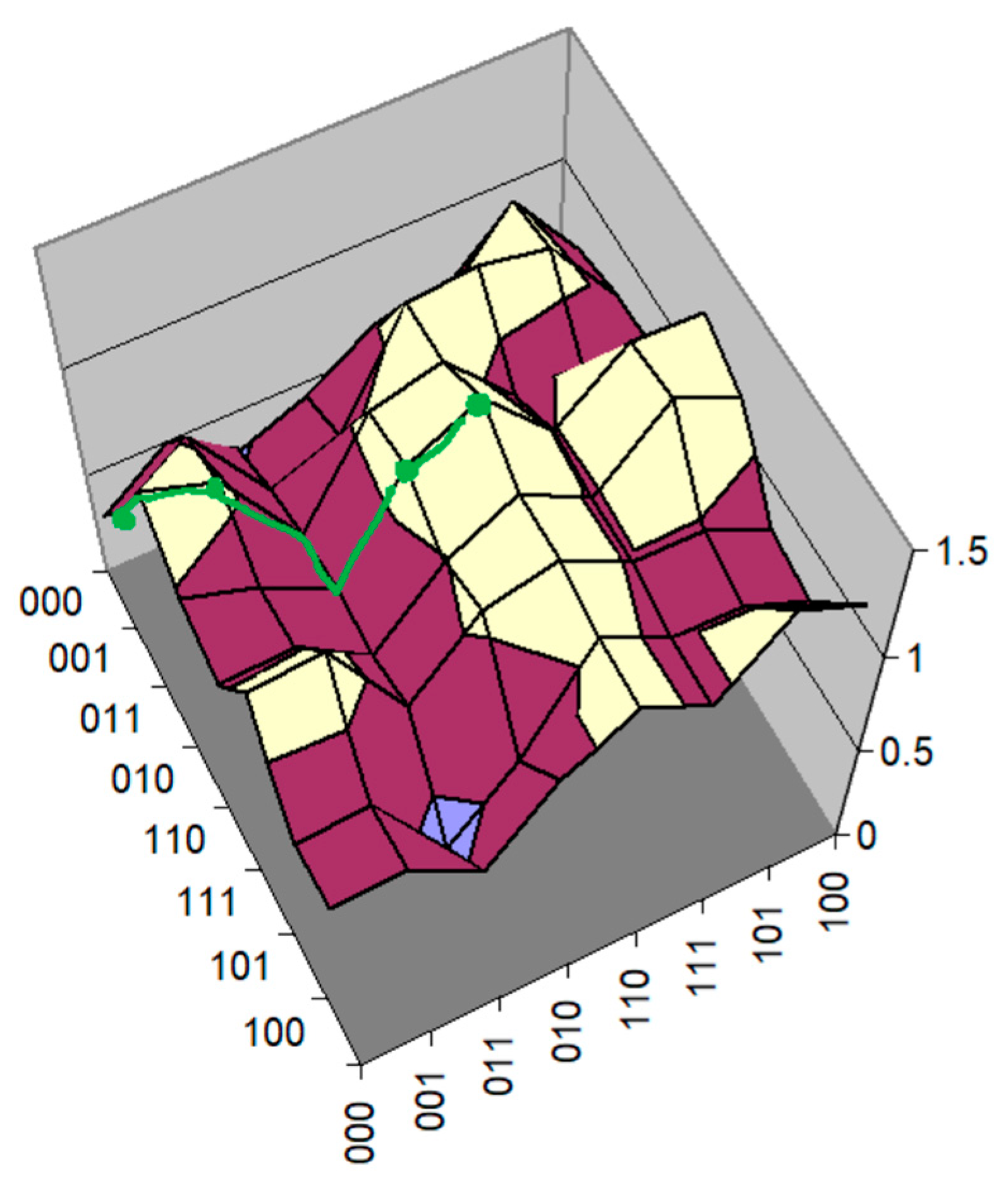
4. Search Algorithms

The objective of the search is to find the highest-performing ‘peak.’ The researcher can use various search algorithms, from naïve search (i.e., random moves) to more realistic search algorithms, that capture the behaviors of single or multiagents. In most applications, search on NK landscapes has a single agent, or if it has multiple agents, the agents are unaware of each other’s movements [46]. Agents communicate only in an NKCS (co-evolutionary system) landscape.

There are three standard search strategies in the literature [47] that have been applied to NK landscapes:

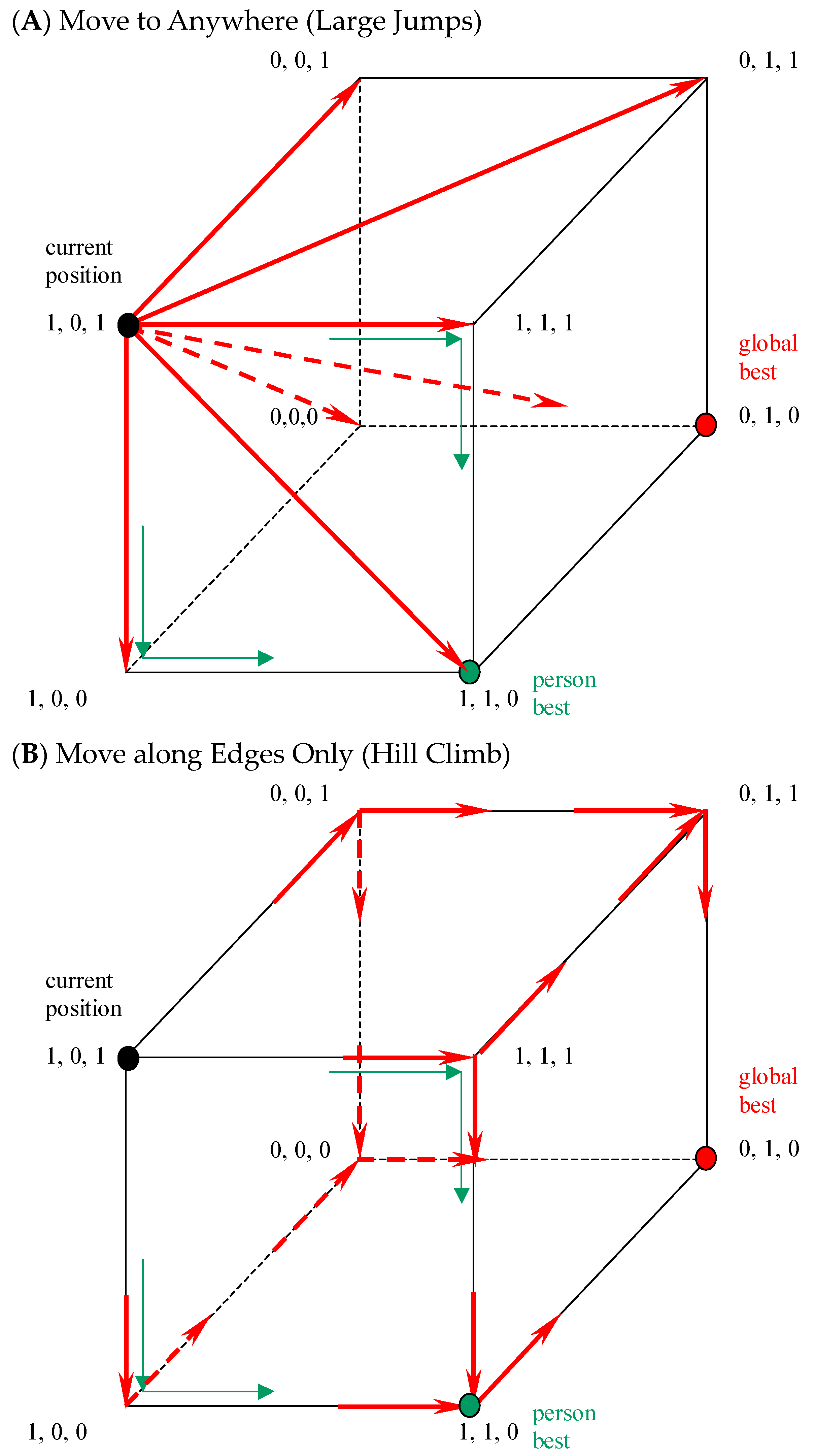
• One-mutant change or hill climb, where an agent chooses a new location from one of its one-mutant neighbors, such as 101 to 001, 111, or 100, if the fitness value of the new location is higher.
• Fitter-dynamics: an agent chooses a new location from the best of its one-mutant neighbors.
• Greedy dynamics (i.e., large or long jump), where an agent chooses a new location from all of its mutant neighbors, whoever has the highest fitness value.

The first two relate to local searches, while the third one relates to distant searches requiring large jumps on the landscape. However, as criticized by Arend (2022), most NK large jumps are achieved by random numbers (i.e., lack of using the knowledge of other firms) [47]. Movements in the swarm model are guided by the intelligence of Equation (5), which include local and large jumps.

Several scholars have studied the NK landscape with similar algorithms to swarm. Wu (2022) uses the directed Erdős–Rényi random network model to study the NK landscape [48]. The Erdős–Rényi network is a special case of the swarm model. It is more limited than the standard swarm model in that each agent can only see partial information about the other agents. Bahceci (2014) uses a memory-based search where agents look for the highest fitness point on the landscape and move along the surface of the landscape based upon their strategy and their memories [11]. This is analogous to swarm in that the former is part of leader following and random exploration and the latter is pursing personal best, both of which are included in (5). In other words, Bahceci’s search algorithm is a special case of swarm intelligence.

Finally, we note that a rich body of literature exists on different search strategies [1,49,50,51,52,53,54]. In this paper, we focus on some standard search strategies to demonstrate swarm search on the NK landscape.

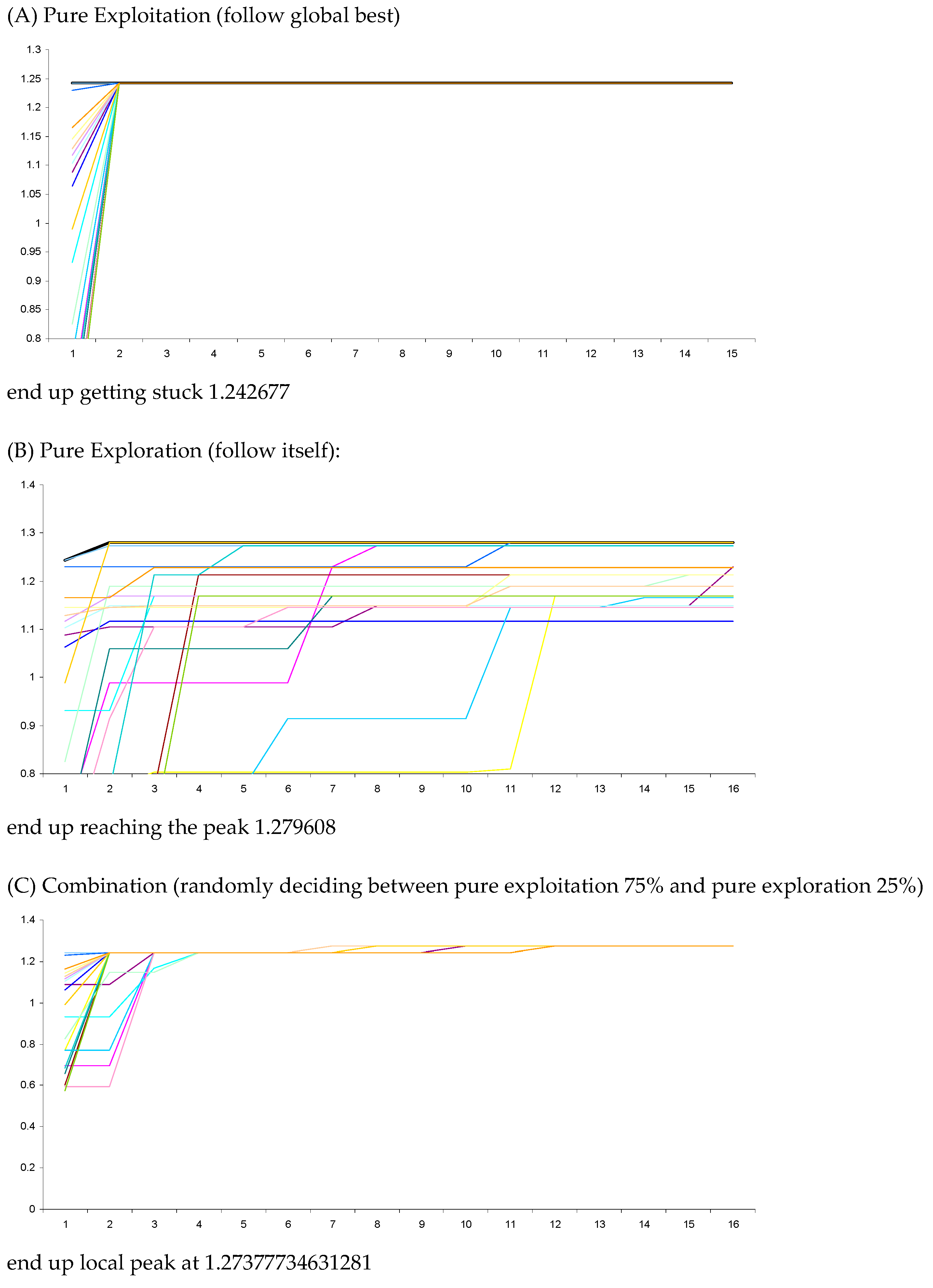
5. Results

Our first experiment is to replicate the work of Ganco and Hoetker (2009) [3]. As in Ganco and Hoetker, we set up a population of $N=6$ with two types of interdependencies: $K=2$ and $K=5$. The former represents a smooth landscape, and the latter a rugged one. The interaction matrix (IM) for $K=2$ is given in (11) and for $K=5$ is given in (11) and (12).

$$I=\begin{array}{cc}& x_1{x}_2{x}_3{x}_4{x}_5{x}_6\\ \begin{array}{l}{x}_1\\ x_2\\ x_3\\ x_4\\ x_5\\ x_6\end{array}& \left[\begin{array}{cccccc}1& 1& & & & 1\\ 1& 1& 1& & & \\ & 1& 1& 1& & \\ & & 1& 1& 1& \\ & & & 1& 1& 1\\ 1& & & & 1& 1\end{array}\right]\end{array}$$

(11)

$$I=\begin{array}{cc}& x_1{x}_2{x}_3{x}_4{x}_5{x}_6\\ \begin{array}{l}{x}_1\\ x_2\\ x_3\\ x_4\\ x_5\\ x_6\end{array}& \left[\begin{array}{cccccc}1& 1& 1& 1& 1& 1\\ 1& 1& 1& 1& 1& 1\\ 1& 1& 1& 1& 1& 1\\ 1& 1& 1& 1& 1& 1\\ 1& 1& 1& 1& 1& 1\\ 1& 1& 1& 1& 1& 1\end{array}\right]\end{array}$$

(12)

To compute any fitness value, Equation (13) is computed as follows (where each component is only affected by two other components):

$$\begin{array}{r}\varphi (x_1,\cdots ,x_6)={\varphi }_1(x_1,x_2,x_6)+{\varphi }_2(x_2,x_1,x_3)+{\varphi }_3(x_3,x_2,x_4)+{\varphi }_4(x_4,x_2,x_3)\\ +{\varphi }_5(x_5,x_4,x_6)+{\varphi }_6(x_6,x_1,x_5)\end{array}$$

(13)

While (14) is computed as follows (where each component is affected by all other 5 components):

$$\varphi (x_1,\cdots ,x_6)={\displaystyle {\sum }_{i=1}^6}{\varphi }_i(x_1,\cdots ,x_6)$$

(14)

Hence, in each of the sub-fitness tables, there will be $2^3=8$ values, each of which is randomly drawn from a uniform distribution. For (15), they are:

$$\begin{array}{l}{\varphi }_1(0,0,0)=u_{1,1}\\ {\varphi }_1(0,0,1)=u_{1,2}\\ {\varphi }_1(0,1,0)=u_{1,3}\\ {\varphi }_1(0,1,1)=u_{1,4}\\ {\varphi }_1(1,0,0)=u_{1,5}\\ {\varphi }_1(1,0,1)=u_{1,6}\\ {\varphi }_1(1,1,0)=u_{1,7}\\ {\varphi }_1(1,1,1)=u_{1,8}\end{array}\begin{array}{l}{\varphi }_2(0,0,0)=u_{2,1}\\ {\varphi }_2(0,0,1)=u_{2,2}\\ {\varphi }_2(0,1,0)=u_{2,3}\\ {\varphi }_2(0,1,1)=u_{2,4}\\ {\varphi }_2(1,0,0)=u_{2,5}\\ {\varphi }_2(1,0,1)=u_{2,6}\\ {\varphi }_2(1,1,0)=u_{2,7}\\ {\varphi }_2(1,1,1)=u_{2,8}\end{array}\cdots \begin{array}{l}{\varphi }_6(0,0,0)=u_{6,1}\\ {\varphi }_6(0,0,1)=u_{6,2}\\ {\varphi }_6(0,1,0)=u_{6,3}\\ {\varphi }_6(0,1,1)=u_{6,4}\\ {\varphi }_6(1,0,0)=u_{6,5}\\ {\varphi }_6(1,0,1)=u_{6,6}\\ {\varphi }_1(1,1,0)=u_{6,7}\\ {\varphi }_1(1,1,1)=u_{6,8}\end{array}$$

(15)

where $u_{i,j}$ is a uniform number for function $i$ and the order of binary $j$. Given a binary number, say 011, we can translate it to a decimal number of 3, which is the 4th random number. We use a fixed seed, and all the random numbers are precalculated. For (16), there are $2^6=64$ values as follows:

$$\begin{array}{lll}{\varphi }_1(0,0,0,0,0,0)=u_{1,1}& & {\varphi }_6(0,0,0,0,0,0)=u_{6,1}\\ {\varphi }_1(0,0,0,0,0,1)=u_{1,2}& & {\varphi }_6(0,0,0,0,0,1)=u_{6,2}\\ \hspace{1em}⋮& \cdots & \hspace{1em}⋮\\ {\varphi }_1(1,1,1,1,1,1)=u_{1,64}& & {\varphi }_6(1,1,1,1,1,1)=u_{6,64}\end{array}$$

(16)

As mentioned earlier, it is common to collapse the hypercube into a three-dimensional graph. We follow Ganco and Hoetker (2009) to plot the result in Figure 5.

As argued by Bahceci (2014), there is no clear systematic way to perform this task. As we can see, Ganko and Hoetker (2009) simply randomly arrange the x-axis to be the first three variables ($x_1~x_3$) and y-axis the last three variables ($x_4~x_6$) with no particular order. As a consequence, it is difficult to see the smoothness and ruggedness. Panel A of Figure 5 is $N=6$ and $K=2$ (smooth), and Panel B of Figure 5 is $N=6$ and $K=5$ (rugged).

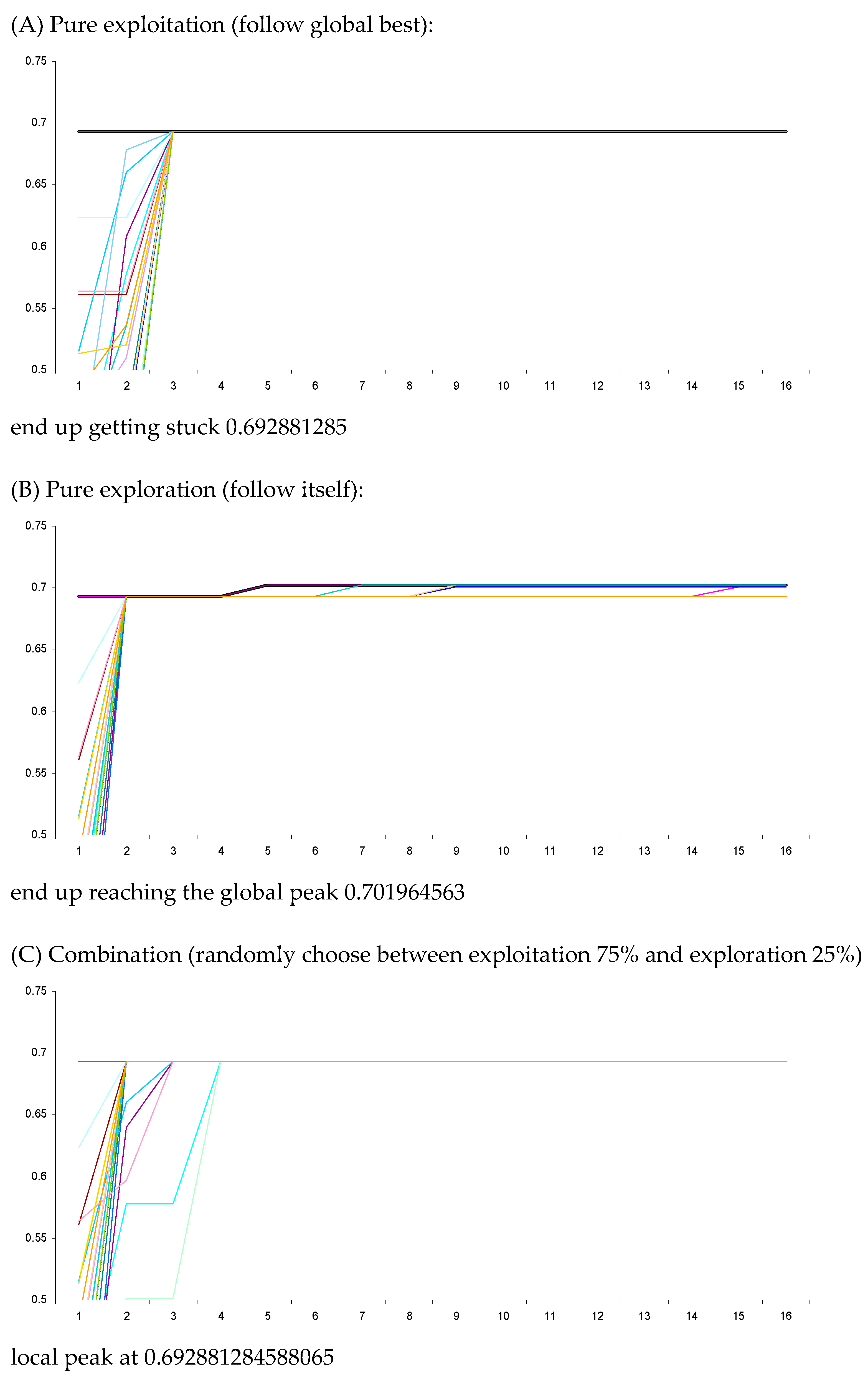
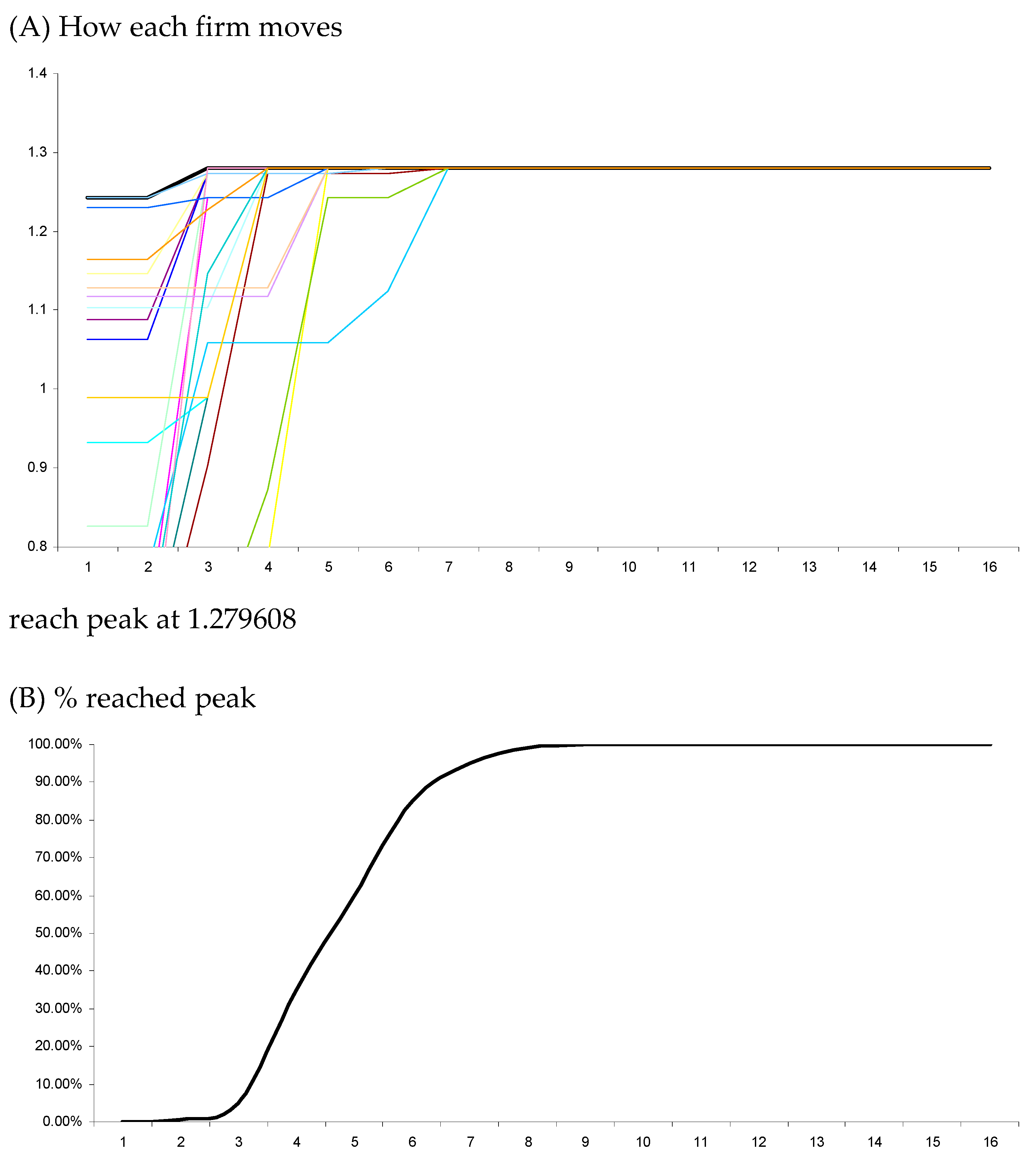
5.1. Global Search

Now we start our swarm simulations. In the first set of simulations, we allow for large jumps (i.e., global search). Each firm can see all the positions (hence fitness values) of other firms. In other words, all firms can see the entire landscape.

The NK landscape is simulated as described in the previous section. The sorted values are plotted in Figure 6. The global peak is 1.279608, positioned at {0, 1, 0, 1, 1, 0}. We also note that the 95th percentile (roughly the 4th highest observation) is 1.229603 positioned at {1, 0, 0, 1, 0, 1}, and the 90th percentile (roughly the 7th highest observation) is 1.189652 positioned at {1, 1, 1, 0, 0, 0}.

The maximum value (global peak) is 1.279608. The 95th percentile (roughly the 61st observation) is 1.229603, and the 90th percentile (roughly the 58th observation) is 1.189652.

Seeing the entire landscape, each firm then decides how to move. There are three possible choices for moving. One, the firm can follow the global best position of the other firms, which we call pure exploitation as the firm is purely exploiting its information gained from the environment. Two, the firm can forge its own path by exploring the landscape on its own, which we call exploration. Third, the firm can randomly toggle between exploration and exploitation, like in a multiarmed bandit model.

We use 20 firms and stop after 16 iterations. The initial position of each firm is randomly generated, and the fitness value is calculated. The results are reported in Figure 7.

Panel A of Figure 7 presents the result of pure exploitation. In this simulation, every firm seeks to move toward the best fitness among its peers. As we can see, in two iterations, all fish stop moving as they all reach a local peak of 1.242677 (the third highest fitness level, see Figure 6) as opposed to a global peak of 1.279608. This is because each firm can jump to the best position quickly. Since this happens so quickly, without exploration, everyone stops.

Panel B of Figure 7 presents the result of pure exploration. However, a firm will only move if a new position is better than its current one (i.e., firms have memory). We can see that all firms move toward the global peak, which is 1.279608. Given that there are only 64 nodes but there are 20 firms, it is understandable that one firm will very soon find the peak, and eventually every firm will find the peak.

Panel C presents the results of the random combination of exploration and exploitation. We set 75% for exploitation and 25% for exploration and each firm randomly choosing between the two. We reach a local peak at 1.273777 (the second-best fitness value, see Figure 6). This is in between pure exploitation and pure exploration, as expected. It is clear by looking at Panel C that exploitation brings very quickly every firm to 1.242677, but instead of getting stuck there, after six iterations, one firm finds a higher position in the landscape and brings everyone else there. Hence, all firms will end up at the global peak.

In terms of visualizing the climbing along the landscape as commonly depicted in the literature, such as Figure 3B, we plot firm #4 in Figure 8.

Figure 8 is the same landscape as Figure 5A, with the path of firm #4 marked. The positions through which firm #4 travels are given below the graph. It is clear that the collapsed landscapes given in Figure 7 do not provide an accurate description of the exact path on which each firm travels.

Next, we present the results of $N=6$ and $K=5$, which we report in Figure 9. Similar to Figure 7, there are three panels for pure exploitation, pure exploration, and combination.

In this case, the landscape is extremely rugged. Again, only pure exploration can reach the peak, which is shown in Figure 9B. Like the previous result, pure exploitation (Figure 9A) is stuck at a local peak for similar reasons. Finally, the combination will eventually reach the global peak (Figure 9C).

One interesting observation is the contrast between Figure 7B and Figure 9B, where the case of pure exploration is present in both landscapes. In a smooth landscape, such as Figure 7B, each firm reaches the global peak gradually and slowly. This is expected, as neighborhoods are just slightly better than the current position. On the contrary, in the case of a rugged landscape, large improvements in fitness can be very nearby, and hence jumps in fitness are more likely. Furthermore, the global peak is likely to be just nearby (for some firms). This is observed in Figure 9B.

Another interesting observation from Figure 9B is that many firms seem to get stuck for a long time before they move. We see this after step 4. The green firm takes a move in step 6, the brown firm in step 8, and the red firm in step 15. There are still many other firms that have not moved at all. This is reasonable, as the landscape is rugged.

One puzzling observation of Figure 9B is that all firms seem to have large jumps to the same location at the very beginning (steps 1~3). This could be just coincidental (it is a simulation, after all).

As a conclusion, we find that exploration outperforms exploitation. This is consistent with the finding by Wu (2022) [47]. This indicates that, in a high-dimensional NK landscape, following peers too closely is very likely to land on a local peak.

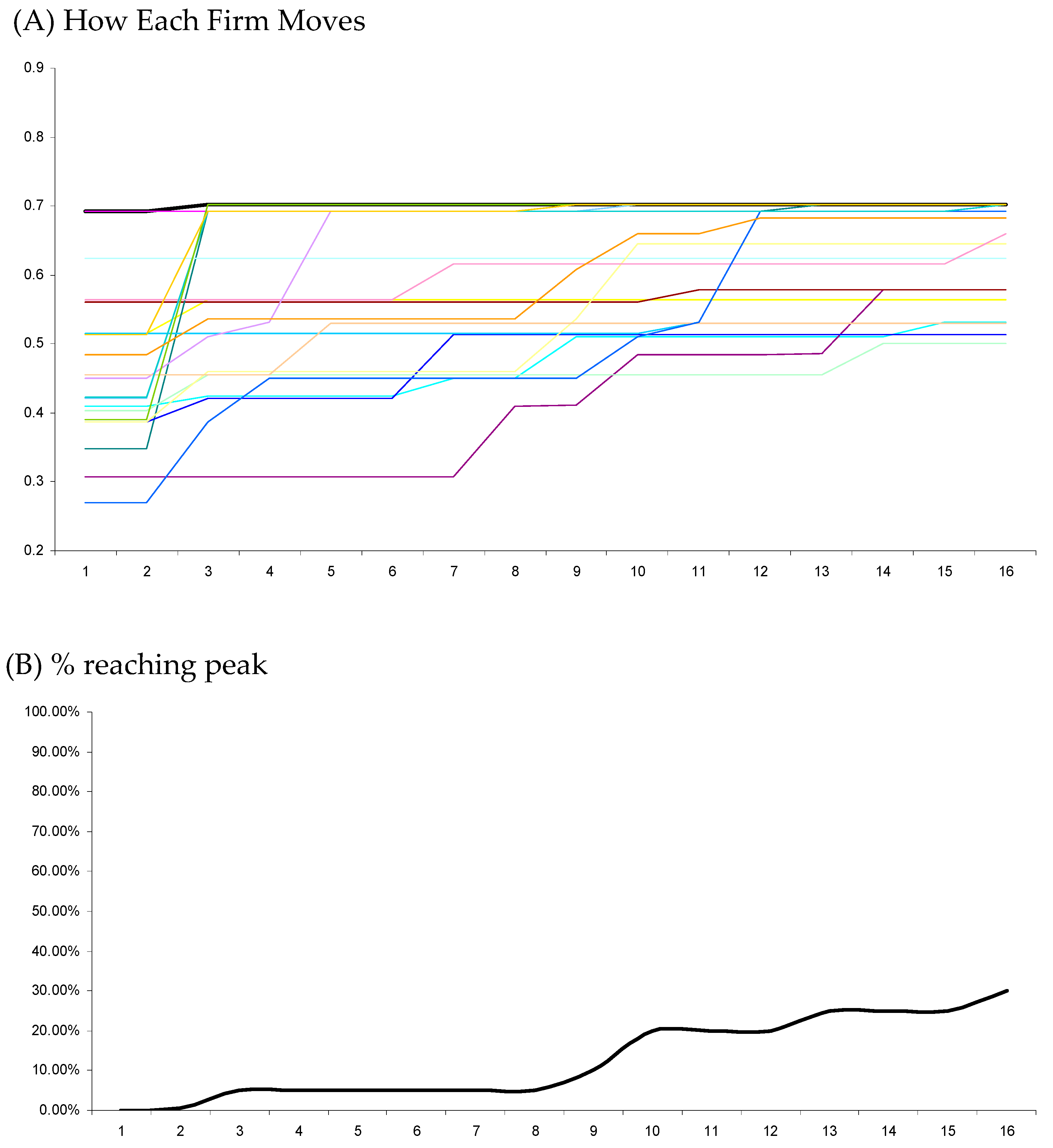
5.2. Local Search

In this sub-section, we provide the results of a local (one-mutant) search. Each firm can still see the global best but cannot move there in one step. Instead, it must move to its immediate neighbor position. For example, 101 can only move to 001, 111, or 100. The main two reasons for such a constraint are that jumps are costly, and firms are not easily (politically or economically) able to perform large jumps. While one could incorporate costs for large jumps (with cost made proportional to distance in a linear or nonlinear fashion), in this paper, for the sake of demonstrating swarm performance, we treat them as two separate cases. It is understandable that once jump costs are prohibitively high, firms will choose to only perform local searches, and on the other extreme, when jumps are free, firms may pursue large jumps (however, as we see in the previous sub-section, large jumps may not end up at the global optimum).

The simulations in this sub-section are only conducted using a combination of both exploitation and exploration. The result for the smooth landscape ($N=6$ and $K=2$) is reported in Figure 10.

As in Figure 9C, Figure 10A shows that firms gradually reach their peak. Due to slower and more gradual movements, it takes longer for all firms to reach the global maximum. Following the literature, we now plot the percentage of firms reaching the global peak in Figure 10B. This is similar to the literature in that the curve is concave right before every firm reaches its peak. Different from the literature, we find that the curve is convex at the beginning.

We display the result for the rugged landscape ($N=6$ and $K=5$) in Figure 11.

Not surprisingly, in the case of a rugged landscape, it takes longer to research the global peak. This can be easily seen by comparing Figure 10 and Figure 11. In Figure 10, all firms reach the global peak at step 7, and yet in Figure 11, less than 10% of firms reach the peak by step 7. Even by step 16 (the maximum number of iterations in our simulations), only 40% can reach the global peak (see Figure 11B). Eventually, all firms will reach the global peak if given enough time.

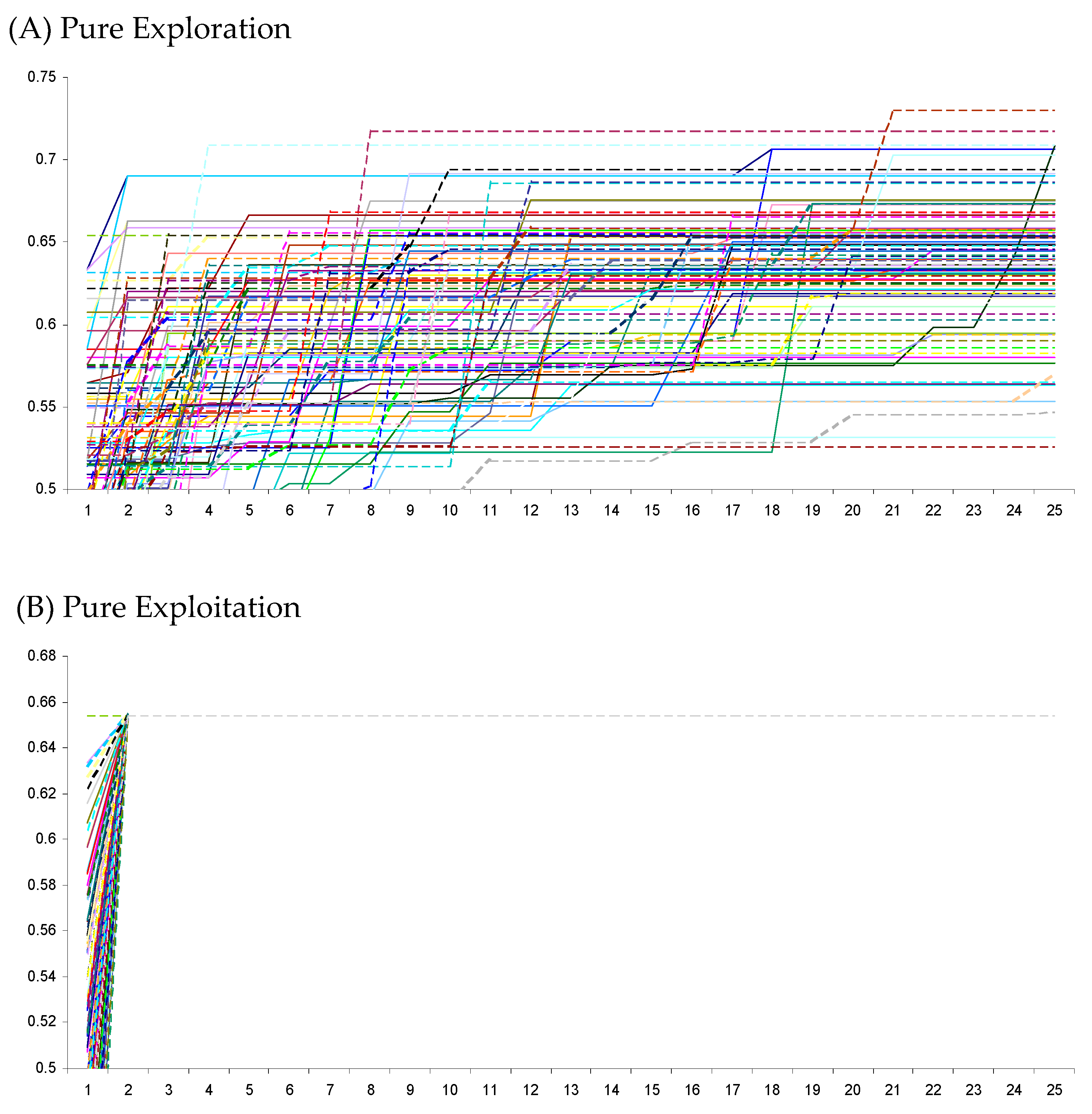
5.3. Large N

In this sub-section, we simulate large samples to see if the results change as compared to small samples. In the literature, researchers typically do not set N to be greater than 20, because at N = 20, the hypercube has a dimension of 2²⁰ = 1,048,576. In our simulations, we use N = 15. We also increase the number of firms to 100, which is a much smaller amount compared to the large space of over 1 million dimensions. As for K, we perform simulations for two cases: K = 14, the most rugged landscape, and the other is a randomly chosen K. In the latter case, we randomly choose K by setting a 50% chance that any other component has an influence on or not on component $i$. Specifically, for a component $i$, we randomly decide if any component $j\ne i$ has an influence or not on component $i$. Hence, on average, K is roughly 7. While we can make the landscape smoother, the result already seems quite conclusive, hence indicating no such need for a smoother landscape.

We present the results for the smooth case in Figure 12 and for the rugged case in Figure 13. Panel A of both figures depicts the case of pure exploration, and Panel B of both figures depicts the case of pure exploitation. We can see that Figure 12 and Figure 13 mimic the results of the previous one with a smaller N. In the case of a smooth landscape (Figure 12, as compared with Figure 7), pure exploration can bring everyone to the peak, yet more slowly when the landscape is larger. And in the case of pure exploitation, firms stop searching very quickly, an identical result found in the smaller landscape. In the case of an extremely rugged landscape (Figure 13, as compared with Figure 9), the situation is the same, which shows that firms do not jump to the global peak at 0.673668.

To conclude, the larger landscape does not provide any more insight than the smaller landscape in Ganco and Hoetker (2009). This is due to the nature of the landscape—a hypercube with binary choices. When a firm searches such a landscape, there is not much flexibility for the firm to move along the hypercube—it can either rely upon its own experience or it follows the leader of the group. Therefore, with such limited choices, larger or smaller landscapes do not make a difference. We conjecture that the sub-group arguments made in the literature also make no substantial differences. Instead, one must include other considerations, such as the differential costs of various choices, to alter the results. We summarize the results and discuss the limitations and opportunities for further development in the following two sections.

6. Discussion of Simulation Results and Identification of Limitations of the NK Landscape for Swarm-Based Search

6.1. Discussion of Simulation Results

We run multiple simulations comparing exploration and exploitation search strategies on smooth and rugged landscapes and with a small and large number of firms. We also examine performance when firms are restricted to one-mutant search strategies. We label following the global best as “exploitation” and randomly exploring on its own as “exploration”. Exploration tends to outperform exploitation if gauged by the probability of a focal firm reaching the highest peak or the number of firms reaching the highest peak. If we take a snapshot at some intermediate point in the simulation (say t = 10), then exploitation typically creates the highest value for firms on average, as firms quickly converge to the best-known location (in terms of payoff), which is unlikely to be the global maximum but may be higher than a random location on the hypercube. Overall, the results may not be that surprising. Early in the simulation run, firms gain more information by copying other firms (maximizing over N other locations) as compared to exploring randomly, so exploitation performs better but will likely result in the firm finding a local rather than global optima.

While we can technically discuss which search strategy performs best under a given set of criteria, it is unclear if such an assessment has practical meaning to the study of firm search due to the limitations the NK landscape places on our swarm model, specifically the use of only one information input from firms rather than a more sophisticated set of inputs (as given in Equations (6) and (7)). The one information input we used was the global best position from the entire firm population. While we could choose some other formulation (a different reference set, etc.), the main limitation is that we can only use one factor rather than multiple factors. The swarm model that we present in Equations (6) and (7) provides a rich way to capture a variety of influences from the environment. These equations can be modified in a variety of ways to capture realistic behaviors. Using the NK landscape, the way swarm can model influences from other firms is too simplistic.

6.2. Further Discussion of NK Limitations for Swarm-Based Search Studies

Prior literature has made extensive use of the NK landscape to represent a combination of interdependent decisions. By modeling each decision as a binary choice that can have interdependencies with other (binary) choices, modelers using NK have produced numerous insights about firms’ or individuals’ search behaviors, which have greatly benefited the strategy and organization literature. While the simplicity of the NK landscape—the hypercube of binary coordinates—is arguably one of its strengths, it also creates several limitations.

First, the NK landscape seems more ideally suited for examining the performance feedback-driven search of one agent rather than how multiple agents influence each other’s search through multiple variables, which is the main application and advantage of swarm in the search literature. NK forces the agent to move along the (0/1) nodes of the hypercube rather than in a real-dimensional space. Therefore, models that take multiple variables (like in Equation (7)) and inform the agent’s search through a weighted average (like in Equation (6)) cannot be fully utilized and instead collapse to one variable input. The ability to draw nuanced inferences about competitive interactions (e.g., imitation, differentiation, etc.) from search is thereby eliminated, which constrains the swarm model’s ability to address interesting search problems.

Second, in our application of the NK landscape, we assume that all firms face the same performance landscape, which may not be realistic. Returns to a position on the landscape could be a function of other firm factors, such as unique resources and capabilities, not captured in the simulation model. This poses no problem for most researchers who apply NK to model one agent’s search but could make multiagent search unrealistic if agents are heterogeneous. Note that such a problem is not specific to NK landscapes but is true for any payoff structure that does not vary across agents. Nevertheless, to make the best use of swarm, a more flexible performance landscape structure is needed.

Overall, the benefits of the NK landscape for individual search limit its ability to appropriately capture a landscape suitable for multiagent search where agents influence each other’s search trajectories through multiple variables.

7. Directions for Future Research

In this section, we discuss how future research can address gaps in swarm modeling as applied to firm search.

7.1. The Need for a Flexible Landscape

The stylized 3-D representation of the NK landscape, as seen in Figure 3, depicts landscapes of different ruggedness, and this stylized view provides powerful insights into the challenges of search. To reap the benefits of swarm models in their application to firm search, researchers need a way to create multidimensional landscapes that can capture the same essence of ‘varying ruggedness’ but can be searched by multiple agents in a continuous way. Those in computer science or related fields that work on search algorithms can contribute to the strategy and management science literature by developing methods of creating such landscapes. Some scholars have begun to examine this problem [55].

7.2. Landscape and Search Process Extensions

Researchers interested in firm/agent search could benefit from the development of several extensions to performance landscapes and search processes. Below, we call for several extensions that, when combined with swarm, could allow the model to better illuminate the challenges of developing search strategies in the real world.

7.2.1. Endogenous Landscapes

From our understanding, the prior literature using search simulations has only considered exogenously given payoffs or performance landscapes. In such work, users generate a landscape based on some parameters and then analyze the search on the landscape. The agent’s position on the landscape does not affect the payoff, which of course makes sense for many of the research questions in which single agent search has been applied. In the analysis of multiagent search, it can make sense for agent positions to alter the payoffs. Consider simulating a firm search across innovation topics, according to Chen et al. (2023). One might expect that the more firms that develop products using the same knowledge, the lower the returns on using such knowledge. From the perspective of the performance landscape, the height of the hill (payoff) falls as more agents take a position on the hill. Endogenizing the landscape in this way can allow researchers to examine more nuanced strategies that better reflect the reality of market competition.

7.2.2. Agent-Specific Landscapes

As discussed in the limitations section above, it is unrealistic to believe that firms with varying endowments of resources and capabilities will perform in the same way by taking the same position on the landscape. To incorporate heterogeneity in the search–performance relationship without directly modeling the heterogeneity, future work could model each agent (firm) on their own landscape. Information about other agents and their payoffs in their own landscapes could be incorporated into the focal agent’s search in its own landscape. Such an approach could illuminate questions regarding whether incorporating information on rivals benefits the focal firm’s search strategy when the extent to which payoffs to the same position vary across firms.

7.2.3. Incomplete Information

Swarm search typically allows the agent to absorb information from a reference group in its complete form. In other words, the agent has complete information on the location and performance of those in the reference group (i.e., F in Equation (7)). In reality, the focal firm is unlikely to know the exact performance of those in the reference group or to be able to link the position in space (e.g., position in knowledge space) to the performance of the firm. Therefore, adding noise to the signal through a random error term or devising other means of making the signal incomplete could have useful applications to the study of search under uncertainty.

7.2.4. Costly Movements

To our knowledge, most search papers allow for the costliest movements across the landscape. In the application of firm search for technological innovations, moving across knowledge topics or technologies is not costless. Incorporating costs could have several benefits. First, incorporating costly movement into the model can allow researchers to better compare search strategies that incur different costs. For instance, local search—searching in the neighborhood of the firm’s location on the landscape—could be less costly than distant search—searching in faraway neighborhoods—as the costs of discovery of new (to the firm) knowledge likely vary based on the firm’s current knowledge stock (as given by the firm’s current and prior positions on the landscape). Second, firms may differ in their cost of search due to their unique external factors (e.g., firm-specific access to the labor market or their own cost of capital) or internal factors (e.g., firm-specific resources and capabilities). Optimal search strategies may differ as these factors differ, and a cost function could allow the researcher to easily incorporate such elements into the model framework. Third, budget constraints could be combined with costs to simulate a resource-constrained search.

8. Conclusions

Recent work by Chen et al. (2023) proposes using swarm-bases search to examine how competitors influence search. Although Chen et al. demonstrate how to fit swarms to data, many problems related to competitive dynamics and search will be better examined with simulation. However, the literature has not considered how to best build a landscape to study firm search with swarms. We apply swarm search to the workhorse landscape model in strategy and organizational search literature—NK. While scholars have generated many valuable insights into firm decision problems using search on NK landscapes, we find that it is not well suited for swarm. We discuss these limitations and identify multiple research opportunities to improve landscapes as well as other features that could improve swarm’s ability to address search problems. We hope to encourage those working with algorithms, such as scholars in computer science and related fields, to help develop tools that can be applied to firm and agent choice problems.

References

- Buamann, O.; Schmitd, J.; Stieglitz, N. Effective search in rugged performance landscapes: A review and outlook. J. Manag. 2019, 45, 285–318. [Google Scholar] [CrossRef]
- Levinthal, D.A.; Marengo, L. Simulation modelling and business strategy research. In The Palgrave Encyclopedia of Strategic Management; Palgrave Macmillan: London, UK, 2018; pp. 1–5. [Google Scholar]
- Ganco, M.; Hoetker, G. NK modeling methodology in the strategy literature: Bounded search on a rugged landscape. In Research Methodology in Strategy and Management; Emerald Group Publishing Limited: Bingley, UK, 2009; Volume 5, pp. 237–268. [Google Scholar] [CrossRef]
- Csaszar, F.A. A note on how NK landscapes work. J. Organ. Des. 2018, 7, 15. [Google Scholar] [CrossRef]
- Chen, R.-R.; Miller, C.D.; Toh, P.K. Modeling firm search and innovation trajectory using swarm Intelligence. Algorithms 2023, 16, 72. [Google Scholar] [CrossRef]
- Kauffman, S.; Levin, S. Towards a general theory of adaptive walks on rugged landscapes. J. Theor. Biol. 1987, 128, 11–45. [Google Scholar] [CrossRef]
- Kauffman, S.; Weinberger, E. The NK Model of rugged fitness landscapes and its application to the maturation of the immune response. J. Theor. Biol. 1989, 141, 211–245. [Google Scholar] [CrossRef]
- Levinthal, D.A. Adaptation on Rugged Landscapes. Manag. Sci. 1997, 43, 934–950. [Google Scholar] [CrossRef]
- Kaul, H.; Jacobson, S.H. Global optima results for the Kauffman NK model. Math. Program. 2005, 106, 319–338. [Google Scholar] [CrossRef]
- Rivkin, J.W.; Siggelkow, N. Patterned interactions in complex systems: Implications for exploration. Manag. Sci. 2007, 53, 1068–1085. [Google Scholar] [CrossRef]
- Bahceci, E. Competitive Multi-Agent Search. Ph.D. Dissertation, University of Texas at Austin, Austin, TX, USA, December 2014. [Google Scholar]
- Beni, G.; Wang, J.; Iglesias, A. Swarm Intelligence in Cellular Robotic Systems. In Proceedings of the NATO Advanced Workshop on Robots and Biological Systems, Tuscany, Italy, 26–30 June 1989; Springer: Berlin/Heidelberg, Germany, 1989; pp. 703–712. [Google Scholar] [CrossRef]
- Bonabeau, E.; Dorigo, M.; Theraulaz, G. Swarm Intelligence: From Natural to Artificial Systems; OUP: Cary, NC, USA, 1999. [Google Scholar]
- Beni, G. Swarm Intelligence. In Encyclopedia of Complexity and Systems Science; Meyers, R.A., Ed.; Springer: New York, NY, USA, 2009; pp. 1–32. [Google Scholar] [CrossRef]
- Reynolds, C. Flocks, herds and schools: A distributed behavioral model. In SIGGRAPH ’87, Proceedings of the 14th Annual Conference on Computer Graphics and Interactive Techniques, Anaheim, CA, USA, 27–31 July 1987; Association for Computing Machinery: New York, NY, USA, 1987; pp. 25–34. [Google Scholar]
- Eberhart, R.; Kennedy, J. Particle swarm optimization. In Proceedings of the IEEE International Conference on Neural Networks, Perth, WA, Australia, 27 November–1 December 1995; Volume 4, pp. 1942–1948. [Google Scholar]
- Shi, Y.; Eberhart, R.C. A modified particle swarm optimizer. In Proceedings of the IEEE International Conference on Evolutionary Computation, Anchorage, AK, USA, 4–9 May 1998; pp. 69–73. [Google Scholar]
- Woodside-Oriakhi, M.; Lucas, C.; Beasley, J. Heuristic algorithms for the cardinality constrained efficient frontier. Eur. J. Oper. Res. 2011, 213, 538–550. [Google Scholar] [CrossRef]
- Zhu, H.; Wang, Y.; Wang, K.; Chen, Y. Particle swarm optimization (PSO) for the constrained portfolio optimization problem expert systems with applications. Exp. Syst. Appl. 2011, 38, 10161–10169. [Google Scholar] [CrossRef]
- Cura, T. Particle swarm optimization approach to portfolio optimization. Nonlinear Anal. Real World Appl. 2009, 10, 2396–2406. [Google Scholar] [CrossRef]
- Raei, R.; Alibeiki, H. Portfolio optimization using particle swarm optimization method. Financ. Res. J. 2010, 12, 1–20. [Google Scholar]
- Thakkar, A.; Chaudhari, K. A comprehensive survey on portfolio optimization, stock price and trend prediction using particle swarm optimization. Arch. Comput. Methods Eng. 2021, 28, 2133–2164. [Google Scholar] [CrossRef]
- Erwin, K.; Engelbrecht, A. Multi-guide set-based particle swarm optimization for multi-objective portfolio optimization. Algorithms 2023, 16, 62. [Google Scholar] [CrossRef]
- Erwin, K.; Engelbrecht, A.P. Set-Based particle swarm optimization for portfolio optimization. In Proceedings of the International Conference on Swarm Intelligence, ANTS Conference, Barcelona, Spain, 26–28 October 2020; pp. 333–339. [Google Scholar]
- Lahmiri, S. Interest rate next-day variation prediction based on hybrid feedforward neural network, particle swarm optimization, and multiresolution techniques. Phys. A Stat. Mech. Its Appl. 2016, 444, 388–396. [Google Scholar] [CrossRef]
- Gao, W.; Su, C. Analysis of earnings forecast of blockchain financial products based on particle swarm optimization. J. Comput. Appl. Math. 2020, 372, 112724. [Google Scholar] [CrossRef]
- Sohrabi, M.; Zandieh, M.; Shokouhifar, M. Sustainable inventory management in blood banks considering health equity using a combined metaheuristic-based robust fuzzy stochastic programming. Socio-Econ. Plan. Sci. 2023, 86, 101462. [Google Scholar] [CrossRef]
- Eberhart, R.C. A discrete binary version of the particle swarm algorithm. In Proceedings of the 1997 IEEE International Conference on Systems, Man, and Cybernetics. Computational Cybernetics and Simulation, Orlando, FL, USA, 12–15 October 1997; pp. 4104–4108. [Google Scholar]
- Lee, S.; Soak, S.; Oh, S.; Pedrycz, W. Modified binary particle swarm optimization. Prog. Nat. Sci. 2008, 19, 1161–1166. [Google Scholar] [CrossRef]
- Di Caro, G. Lecture Notes (Chapter 16 of Collective Intelligence: From Multi-Agent Systems to Swarms); Carnegie Mellon University: Pittsburgh, PA, USA, 2019. [Google Scholar]
- Dehghani, M.; Samet, H. Momentum search algorithm: A new meta-heuristic optimization algorithm inspired by momentum conservation law. SN Appl. Sci. 2020, 2, 1720. [Google Scholar] [CrossRef]
- Nguyen, B.H.; Xue, B.; Andreae, P.; Zhang, M. A new binary particle swarm optimization approach: Momentum and dynamic balance between exploration and exploitation. IEEE Trans. Cybern. 2021, 51, 589–603. [Google Scholar] [CrossRef]
- Shokouhifar, A.; Shokouhifar, M.; Sabbaghian, M.; Soltanian-Zadheh, H. Swarm intelligence empowered three-stage ensemble deep learning for arm volume measurement in patients with lymphedema. Biomed. Signal Process. Control 2023, 85, 105027. [Google Scholar] [CrossRef]
- Kumar, A.; Kumar, S.A.; Dutt, V.; Dubey, A.K.; Garcia-Diaz, V. IoT-based ECG monitoring for arrhythmia classification using Coyote Grey Wolf optimization-based deep learning CNN classifier. Biomed. Signal Process. Control 2022, 76, 103638. [Google Scholar] [CrossRef]
- Mahmoodzadeh, A.; Nejati, H.R.; Mohammadi, M.; Ibrahim, H.H.; Rashidi, S.; Rashid, T.A. Forecasting tunnel boring machine penetration rate using LSTM deep neural network optimized by grey wolf optimization algorithm. Expert Syst. Appl. 2022, 209, 118303. [Google Scholar] [CrossRef]
- Yang, X.; Zhao, D.; Yu, F.; Heidari, A.A.; Bano, Y.; Ibrohimov, A.; Liu, Y.; Cai, Z.; Chen, H.; Chen, X. An optimized machine learning framework for predicting intradialytic hypotension using indexes of chronic kidney disease-mineral and bone disorders. Comput. Biol. Med. 2022, 145, 105510. [Google Scholar] [CrossRef]
- Guerra, J.F.; Garcia-Hernandex, R.; Llama, M.A.; Santibanez, V. A comparative study of swarm intelligence metaheuristics in ukf-based neural training applied to the identification and control of robotic manipulator. Algorithms 2023, 16, 393. [Google Scholar] [CrossRef]
- Tomassetti, G.; Cagnina, L. Particle swarm algorithms to solve engineering problems: A comparison of performance. J. Eng. 2013, 2013, 435104. [Google Scholar] [CrossRef]
- Papazoglu, G.; Biskas, P. Review and comparison of genetic algorithm and particle swarm optimization in the optimal power flow problem. Energies 2023, 16, 1152. [Google Scholar] [CrossRef]
- Kicska, G.; Kiss, A. Comparing swarm intelligence algorithms for dimension reduction in machine learning. Big Data Cogn. Comput. 2021, 5, 36. [Google Scholar] [CrossRef]
- Selvaraj, S.; Choi, E. Survey of swarm intelligence algorithms. In ICSIM ’20, Proceedings of the 3rd International Conference on Software Engineering and Information Management, Sydney, NSW, Australia, 12–15 January 2020; ACM: New York, NY, USA, 2020; pp. 69–73. [Google Scholar] [CrossRef]
- Banerjee, S.; Agarwal, N. Analyzing collective behavior from blogs using swarm intelligence. Knowl. Inf. Syst. 2012, 33, 523–554. [Google Scholar] [CrossRef]
- O’Bryan, L.; Beier, M.; Salas, E. How approaches to animal swarm intelligence can improve the study of collective intelligence in human teams. J. Intell. 2020, 8, 9. [Google Scholar] [CrossRef]
- Minar, N.; Burkahrt, R.; Langston, C.; Askenzi, M. The Swarm Simulation System: A Toolkit for Building Multi-Agent Simulations. Santa Fe Institute Working Paper. 1996. Available online: https://EconPapers.repec.org/RePEc:wop:safiwp:96-06-042 (accessed on 13 October 2023).
- Coen, C.A.; Maritan, C.A. Investing in Capabilities: The Dynamics of Resource Allocation. Organ. Sci. 2011, 22, 99–117. [Google Scholar] [CrossRef]
- Padget, J.; Vidgen, R.; Mitchell, J.; Marshall, A.; Mellor, R. Sendero: An extended, agent-based implementation of Kauffman’s NKCS model. J. Artif. Soc. Soc. Simul. 2009, 12, 1–8. [Google Scholar]
- Arend, R.J. Balancing the Perceptions of NK Modeling with Critical Insights. J. Innov. Entrep. 2022, 11, 23. [Google Scholar] [CrossRef]
- Wu, J. Withholding Knowledge; Department of Logic and Philosophy of Science, University of California at Irvine: Irvine, CA, USA, 2022. [Google Scholar]
- Kauffman, S.A.; Macready, W.G. Search strategies for applied molecular evolution. J. Theor. Biol. 1995, 173, 427–440. [Google Scholar] [CrossRef]
- Merz, P. Memetic Algorithms for Combinatorial Optimization Problems: Fitness Landscapes and Effective Search Strategies. Ph.D. Dissertation, Fachbereich 12, Elektrotechnik und Informatik, Lemgo, Germany, 2006. [Google Scholar]
- Krasnogor, N.; Smith, J. Emergence of profitable search strategies based on a simple inheritance mechanism. In GECCO’01, Proceedings of the 3rd Annual Conference on Genetic and Evolutionary Computation, San Francisco, CA, USA, 7–11 July 2001; ACM: New York, NY, USA, 2001; pp. 432–439. [Google Scholar]
- Bausseur, M.; Goeffon, A.; Lareux, F.; Saubion, F.; Vigneron, V. On the attainability of NK landscapes global optima. In Proceedings of the Seventh Annual Symposium on Combinatorial Search (SoCS 2014), Prague, Czech Republic, 15–17 August 2014; Association for the Advancement of Artificial Intelligence: Washington, DC, USA, 2021; Volume 5, pp. 28–34. [Google Scholar] [CrossRef]
- Geisendorf, S. Searching NK fitness landscapes: On the trade off between speed and quality in complex problem solving. Comput. Econ. 2010, 35, 395–406. [Google Scholar] [CrossRef]
- Li, W.; Meng, X.; Huang, Y. Fitness distance correlation and mixed search strategy for differential evolution. Neurocomputing 2021, 458, 514–525. [Google Scholar] [CrossRef]
- Harrison, J.R.; Kemp, A.; Saetre, A.S. Attraction-based fitness landscapes for computational decision search. In Proceedings of the PICMET ‘17: Technology Management for Interconnected World, PICMET, Portland, OR, USA, 9–13 July 2017. [Google Scholar]
Disclaimer/Publisher’s Note: The statements, opinions and data contained in all publications are solely those of the individual author(s) and contributor(s) and not of MDPI and/or the editor(s). MDPI and/or the editor(s) disclaim responsibility for any injury to people or property resulting from any ideas, methods, instructions or products referred to in the content. |
© 2023 by the authors. Licensee MDPI, Basel, Switzerland. This article is an open access article distributed under the terms and conditions of the Creative Commons Attribution (CC BY) license (https://creativecommons.org/licenses/by/4.0/).
Share and Cite
Chen, R.-R.; Miller, C.D.; Toh, P.K. Search on an NK Landscape with Swarm Intelligence: Limitations and Future Research Opportunities. Algorithms 2023, 16, 527. https://doi.org/10.3390/a16110527
Chen R-R, Miller CD, Toh PK. Search on an NK Landscape with Swarm Intelligence: Limitations and Future Research Opportunities. Algorithms. 2023; 16(11):527. https://doi.org/10.3390/a16110527
Chicago/Turabian StyleChen, Ren-Raw, Cameron D. Miller, and Puay Khoon Toh. 2023. "Search on an NK Landscape with Swarm Intelligence: Limitations and Future Research Opportunities" Algorithms 16, no. 11: 527. https://doi.org/10.3390/a16110527
APA StyleChen, R.-R., Miller, C. D., & Toh, P. K. (2023). Search on an NK Landscape with Swarm Intelligence: Limitations and Future Research Opportunities. Algorithms, 16(11), 527. https://doi.org/10.3390/a16110527