1. Introduction
The use of side information in a supervised machine learning (ML) setting, proposed in [
1], was referred to as
privileged information, and was further developed in [
2], who extended the paradigm to unsupervised learning. As illustrated in [
3], privileged information refers to data which neither belong to the input space nor to the output space but are still beneficial for learning. In general, side information may, for example, be knowledge given by a domain expert.
In our work, side information comes separate to the training and test data, but unlike other approaches such as the one described above, it can be used by the ML algorithm not only during training but also during testing. In particular, we concentrate on supervised neural networks (NNs) and do not constrain the side information to be fed into the input layer of the network, which constitutes a non-trivial extension of the paradigm. To distinguish between the two approaches we refer to the additional information used in the previous approaches, when the information is only visible during the training phase, as privileged information, and in our approach, when the information is visible during both the train and test phases, simply as
side information. In our model, side information is fed into the NN from a knowledge base, which inspects the current input data and searches for relevant side information in its memory. Two examples of the potential use of side information in ML are the use of azimuth angles as side information for images of 3D chairs [
4], and the use of dictionaries as side information for extracting medical concepts from social media [
5].
Here, we present an architecture and formalism for side information, and also a proof of concept of our model on a couple of datasets to demonstrate how it may be useful in the sense of improving the performance of an NN. We note that side information is not necessarily useful in all cases, and, in fact, it could be malicious, causing the performance of an NN to decrease.
Our proposal for incorporating side information is relatively simple when side information is available, and, within the proposed formalism, it is straightforward to measure its contribution to the ML. It is also general in terms of the choice of neural network architecture that is used, and able to cater for different formats of side information.
To reiterate, the main research question we address here is when side information comes separate to the training and test data, what is the effect, on the ML algorithm, of making use of such side information, not only during training but also during testing? The rest of the paper is organised as follows: In
Section 2, we review some related work, apart from the privileged information already mentioned above. In
Section 3, we present a neural network architecture that includes side information, while in
Section 4 we present our formalism for side information based on the difference between the loss of the NN without and with side information, where side information is deemed to be useful if the loss decreases. In
Section 5, we present the materials and methods used for implementing the proof of concept for side information based on two datasets, while in
Section 6 we present the results and discuss them. Finally, in
Section 7, we present our concluding remarks.
2. Related Work
We now briefly mention some recent related research. In [
6], a language model is augmented with a very large external memory, and uses a nearest-neighbour retrieval model to search for similar text in this memory to enhance the training data. The retrieved information can be used during the training or fine-tuning of neural language models. This work focuses on enhancing language models, and, as such, does not address the general problem of utilising side information.
In a broad sense, our proposal fits into the informed ML paradigm with prior information, where prior knowledge is independent from the input data; has a formal representation; and is integrated into the ML algorithm [
7]. Moreover, human knowledge may be input into an ML algorithm in different formats, through examples, which may be quantitative or qualitative [
8]. In addition, there are different ways of incorporating the knowledge into an ML algorithm, say an NN, for example, by modifying the input, the loss function, and/or the network architecture [
9]. Another trend is that of incorporating physical knowledge into deep learning [
10], and more specifically encoding differential equations in NNs, leading to physics-informed NNs [
11].
Our method of using probabilistic facts, described in
Section 3, is a straightforward mechanism for extracting the information that is needed from the knowledge base in order to integrate them into the neural network architecture in a flexible manner. Moreover, our proposal allows feeding side information into any layer of the NN, not just into the input layer, which is to the best of our knowledge novel.
Somewhat related is also neuro-symbolic artificial intelligence (AI), where neural and symbolic reasoning components are tightly integrated via neuro-symbolic rules; see [
12] for a comprehensive survey of the field, and [
13] which looks at combining ML with semantic web components. While NNs are able to learn non-linear relationships from complex data, symbolic systems can provide a logical reasoning capability and structured representation of expert knowledge [
14]. Thus, in a broad sense, the symbolic component may provide an interface for feeding side information into an NN. In addition, a neuro-symbolic framework was introduced in [
15] that supports querying, learning, and reasoning about data and knowledge.
We point out that, as such, our formalism for incorporating side information into an NN does not attempt to couple symbolic knowledge reasoning with an NN as does neuro-symbolic AI [
12,
15]. The knowledge base, defined in
Section 3, acts as a repository, which we find convenient to describe in terms of a collection of facts providing a link, albeit weak, to neuro-symbolic AI. For example, in
Section 5, in the context of the well-known MNIST dataset [
16], we use expert knowledge on whether an image of a digit is peculiar as side information for the dataset, and inject this information directly into the NN, noting that we do not insist the side information exists for all data items.
3. A General Method for Incorporating Side Information
To simplify the model under discussion, let us assume a generic neural network (NN) with input and output layers and some hidden layers in-between. We use the following terminology: is the input to the NN at time step t, is the true target value (or simply the target value), is the estimated target value (or the NN’s output value), and is the side information, defined more precisely below.
The side information comes from a knowledge base, , containing both facts (probabilistic statements) and rules (if–then statements). To start off, herein, we will restrict ourselves to side information in the form of facts represented as triples, , with p being the probability that the instance z is a member of class c, and where a class may be viewed as a collection of facts. In other words, the triple can be written as , which is the likelihood of z given c. We note that facts may not necessarily be atomic units, and that side information such as is generally viewed as a conjunction of one or more facts.
Let us examine some examples of side information facts, demonstrating that the knowledge base can, in principle, contain very general information:
- (i)
is the probability of a headache being a . Here, is a textual instance and the likelihood is .
- (ii)
is the probability that the background of is ; in this case the probability could denote the proportion of the background of the image. Here, is an image instance and the likelihood is .
- (iii)
is the probability that is . Here, is a segment of an ECG time series instance and the likelihood is .
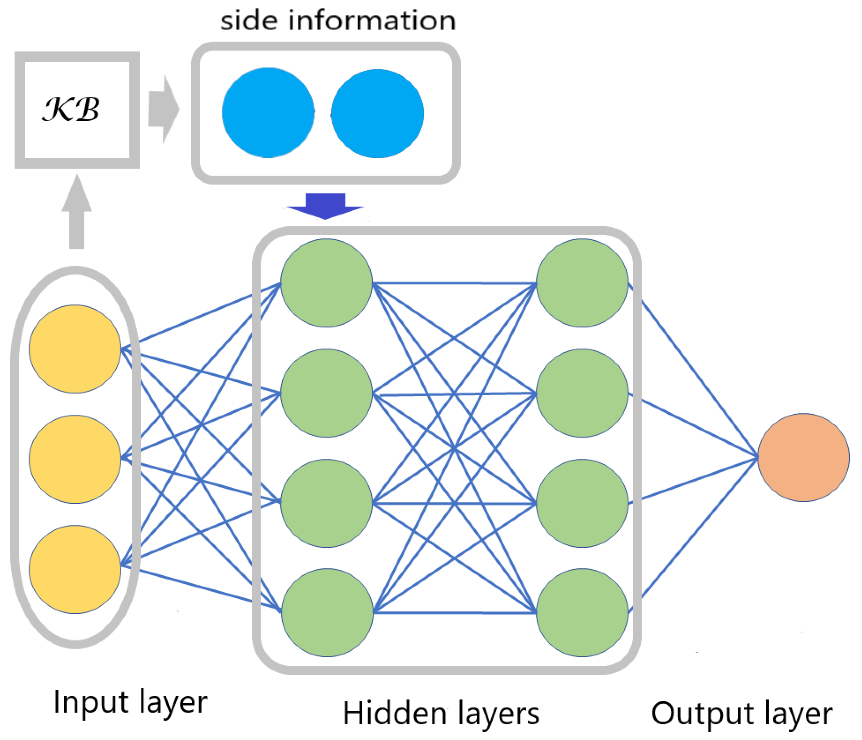
The architecture of the neural network incorporating side information is shown in
Figure 1. We assume that the NN operates in discrete time steps, and that at the current time step,
t, instance
is fed into the network and
is its output. As stated above, we will concentrate on a knowledge base of facts, and detail what preprocessing may occur to incorporate facts into the network as side information. It is important that the preprocessing step at time
t can only access the side information and the input presented to the network at that time, i.e., it cannot look into the past or the future. It is, of course, sensible to assume that one cannot access inputs that will be presented to the network in the future at times greater than
t, and regarding the past, at times less than
t, the reasoning being that this information is already encoded in the network. Moreover, the learner may not be allowed to look into the past due to privacy considerations. On a high level, this is similar to continual learning (CL) frameworks where a CL model is updated at each time step using only the new data and the old model, without access to data from previous tasks due to speed, security, and privacy constraints [
17].
As noted in the caption of
Figure 1, side information may be connected to the rest of the network in several ways through additional nodes. The decision of whether, for example, to connect the side information to the first or second hidden layers and/or also to the output node can be made on the basis of experimental results. We emphasise that in our model, side information is available in both the training and test phases.
Let
be the input instance to the network at time step
t and
represent the side information at time
t, where
is a set of constraints which may be empty. To clarify how side information is incorporated into an NN, we give, in Algorithm 1, high-level pseudo-code corresponding to the architecture for side information, as shown in
Figure 1.
| Algorithm 1 Training or testing with side information |
- 1:
is the input to the network at time step t during the train or test phase - 2:
layer of the network that the side information is fed into - 3:
the set of constraints on the knowledge base - 4:
for time step do - 5:
is fed as input to the network - 6:
- 7:
an encoding of is fed into the network at layer - 8:
output of the network - 9:
end for
|
We stipulate that , i.e., we can either first compute the result of applying to , resulting in , and then constrain to , or, alternatively, we can first constrain to , resulting in , and then apply to . For this reason, from now on, we prefer to write instead of , noting that when is empty, i.e., , then . We leave the internal working of unspecified, although we note that it is important that the computational cost of is low.
The set of constraints may be application-dependent, for example, on whether is text- or image-based. Moreover, for a particular dataset we may constrain knowledge-based queries to a small number of one or more classes. To give a more concrete example, if , i.e., the input to the network is an image, and we have constrained the knowledge base to the class , then its output will be of the form . In this case, the knowledge base matches the input image precisely and returns in its probability of being . In the more general case, the knowledge base will only match part of the input.
More specifically, we let be the result of applying the knowledge base to the input , where each , for , encodes a fact , so that the probability, , for , will be fed to the network as side information. From a practical perspective it will be effective to set a non-negative threshold such that is included in only when .
We also assume for convenience that the number of facts returned by
that are fed into the network as side information is fixed at a maximum, say
m, and that they all pass the threshold, i.e.,
. Now, if there are more than
m facts that pass the threshold, then we only consider the top
m facts with the highest probabilities, where ties are broken randomly. On the other hand, if there are less than
m facts that pass the threshold, say
, then we consider the values for the
facts that did not pass the threshold as missing. A simple solution to deal with the missing values is to consider their imputation [
18], and in particular, we suggest using a constant imputation [
19] replacing the missing values with a constant such as the mean or the median for the class, which will not adversely affect the output of the network. We observe that if
for all inputs
in the test data, but not necessarily in the training data, then side information is reduced to privileged information.
Now, assuming that all the side information is fed directly into the first hidden layer, as is the input data, then it can be shown that using side information is equivalent to extending the input data by m values through a preprocessing step, and then training and testing the network on the extended input. When side information is fed into other layers of the network this equivalence breaks down.
4. A Formalism for Side Information
Our formalism for assessing the benefits of side information is based on quantifying the difference between the loss of the neural network without and with side information; see (
1) below. Additionally, we provide detailed analysis for two of the most common loss functions,
squared loss and
cross-entropy loss [
20]; see (
2) and (
3), respectively, below.
Moreover, in (
5) we present the notion of being
individually useful at time step
t, which is the smallest non-negative
such that the probability that the difference in loss at
t when side information is absent and present is larger than a given non-negative margin,
, which is greater than or equal to
. When side information is individually useful for all time steps it is said to be
globally useful. Furthermore, in (
6) we modify (
5) to allow for the concept of side information being
useful on average.
To clarify the notation, we assume that is the input to the NN at time t, is the target value given input , is the estimated target value given , i.e., the output of the NN when no side information is available for , and is the estimated target value given and side information , i.e., the output of the NN when side information is present for .
To formalise the contribution of the side information, let
be the NN loss on input
and
be the NN loss on input
with side information
. The difference between the loss from
and the loss from
, where
and
, is given by
Now assuming squared loss for a regression problem, we obtain
which has a positive solution when
, i.e., both terms in the last equation are negative, or
, i.e., both these terms are positive.
If we restrict ourselves to binary classifiers, then squared loss reduces to the well-known Brier score [
21]. Inspecting (
2) for this case, when
we have the constraint
, ensuring both terms are negative. Correspondingly, when
, we have the constraint
, ensuring that both terms are positive; note that in this case,
is intuitive since the classifier returns the probability of
being 1, i.e., estimating the chance of a positive outcome.
On the other hand, assuming cross-entropy loss for a classification problem, we obtain
which has a positive solution when
.
In this case, if we restrict ourselves to binary classifiers, then cross-entropy loss reduces to the well-known logarithmic score [
21]. Here, we need to note that a positive solution always exists, since the binary cross-entropy loss is given by
when the estimated target value is
, and similarly replacing
with
when the estimated target value is
.
Now, we would like the probability,
, for
and a given margin,
, for the difference between
and
to be minimised; that is, we wish to evaluate
The probability in (
5) can be estimated by parallel or repeated applications of the train and test cycle for the NN without and with side information, and the losses
and
are recorded for every individual run in order to minimise over
for a given
. Each time the NN is trained its parameters are initialised randomly and the input is presented to the network in a random order, as was done in [
22]; other methods of randomly initialising the network are also possible [
23].
When (
5) is satisfied, then we say that side information is
individually useful for
t, where
. In the case when side information is individually useful for all
we say that side information is (strictly)
globally useful. We define side information to be
useful on average if the following modification of (
5) is satisfied:
noting that we can estimate (
6) in a similar way to estimating (
5) with the difference that, in order to minimise over
for a given
, the average loss is calculated for each run of the NN.
In the case where the greater or equal operator (≥) in the inequality
, contained in (
5), is substituted with equality to zero (
) or is within a small margin thereof (i.e.,
is close to 0), we may say that side information is
neutral. Moreover, we note that there may be situations when side information is
malicious, which can be captured by swapping
and
in (
5). We will not deal with these cases herein and leave them for further investigation. (Similar modifications can be made to (
6) for side information to be neutral or malicious on average.)
We note that malicious side information may be adversarial, i.e., intentionally targeting the model, or simply noisy, which has a similar effect but is not necessarily deliberate. In both cases, the presence of side information will cause the loss function to increase. Here, we do not touch upon the methods for countering adversarial attacks, which is an ongoing endeavour [
24].
5. Materials and Methods
As a proof of concept of our model of side information, we consider two datasets. The first is the
Modified National Institute of Standards and Technology (MNIST) dataset [
16]. It is a handwritten,
pixel image, digit database consisting of a training set of 60,000 instances and a test set of 10,000 instances. These are the standard sizes of training and test for MNIST, which result in about 85.7% of the data being used for training and about 14.3% reserved for testing. This is a classification problem where there are 10 labels each depicting a digit identity between 0 and 9.
Our second experiment is based on the House Price dataset, which is adapted from the Zillow’s home value prediction Kaggle competition dataset [
25], which contains 10 input features as well as a label variable [
26]. The dataset consists of 1460 instances. The main task is to predict whether the house price is above or below the median value according to value of the label variable being 1 or 0, respectively, so it is therefore a binary classification problem.
For both experiments we utilised a
fully connected feedforward neural network (FNN) containing two hidden layers, as well as a softmax output layer; see also
Figure 1 and Algorithm 1 regarding the modification of the neural network to handle side information. Our experiments mainly aim at evaluating whether or not the utilisation of side information is beneficial to the performance of the learning algorithm, i.e., whether it is useful. This is achieved by evaluating the difference between the respective NN losses without and with side information. The experiments demonstrate the effectiveness of our approach in improving the learning performance, which is evidenced by a reduction in the loss (i.e., improvements in the accuracy) of the classifiers, for each of the two experiments, during the test phase.
In both experiments, all the reported classification accuracy values and usefulness estimates (according to (
5) and (
6)) are averaged over 10 separate runs of the NN. For every experiment, we also report the statistical significance values of the differences between the corresponding classification accuracy values, without and with side information. To this effect, we perform a paired
t-test to assess the difference in accuracy levels obtained, where the null hypothesis states that the corresponding accuracy levels are not significantly different.
For each run out of the 10 repetitions, the parameters of the NN are initialised randomly. In addition, the order via which the input data are presented to the network is also randomly shuffled during each run. Also, missing side information values are replaced with the average value of the side information for the respective class label. The number of epochs used is 10, with a batch size of 250. The adopted loss used in both experiments is the cross-entropy loss.
5.1. MNIST Dataset
For this dataset we add side information in the form of a single attribute, giving information about how peculiar the handwriting of the corresponding handwritten digit looks. The spectrum of values is between 0, which refers to a very odd-looking digit with respect to its ground-truth identity, and 1, which denotes a very standard-looking digit; we also made use of three intermediate values, , and . This side information was coded manually for of the test and training data, and was fed into the network through the knowledge base right after the first hidden layer. In accordance with the adopted FNN architecture, we believe that adding side information after the first hidden layer best highlights the utilisation of the proposed concept of side information, since if the side information was to be added prior to that (i.e., before the first layer), its impact would have been equivalent to extending the input. Otherwise, adding it after the second hidden layer (although technically possible) may not enable the side information to sufficiently impact the learning procedure. According to the representation, the side information here can be generated as .
As mentioned earlier, an FNN with two hidden layers is utilised. The first hidden layer consists of 350 hidden units, whereas the second hidden layer contains 50 hidden units (these choices are reasonable given the size and structure of the dataset), followed by a softmax activation. Similar to numerous previous works in ML, we focus on comparisons based on an FNN with a certain capacity (two hidden layers in our case, rather than five or six, for instance) in order to concentrate on assessing the algorithm rather than the power of a deep discriminative model.
5.2. House Price Dataset
The FNN utilised in this experiment consists of two hidden layers, followed by a softmax activation. The first hidden layer consists of 12 hidden units, while the second consists of 4 hidden units (these choices are reasonable given the size and structure of the dataset). A portion of of the data is reserved for the test set.
Out of the 10 features, we experimented with one feature at a time being kept aside. Whilst the other 9 features are presented as input to the input layer of the NN in the normal manner, the aforementioned 10th feature is used to generate side information, which is fed to the NN through the knowledge base right after the first hidden layer. The reasoning behind selecting this location for adding the side information is similar to the one highlighted with MNIST. According to the representation, here, the side information can be generated as , where the feature in question varies according to the one left out.


