Activation Function Dynamic Averaging as a Technique for Nonlinear 2D Data Denoising in Distributed Acoustic Sensors

Abstract

This work studies the application of low-cost noise reduction algorithms for the data processing of distributed acoustic sensors (DAS). It presents an improvement of the previously described methodology using the activation function of neurons, which enhances the speed of data processing and the quality of event identification, as well as reducing spatial distortions. The possibility of using a cheaper radiation source in DAS setups is demonstrated. Optimal algorithms’ combinations are proposed for different types of the events recorded. The criterion for evaluating the effectiveness of algorithm performance was an increase in the signal-to-noise ratio (SNR). The finest effect achieved with a combination of algorithms provided an increase in SNR of 10.8 dB. The obtained results can significantly expand the application scope of DAS.

1. Introduction

Distributed fiber optic sensors are one of the most dynamically developing scientific and technical areas today [1,2,3,4]. Practice shows that they can be used to obtain information regarding the distribution of factors of almost any origin affecting the optical sensor. Distributed fiber optic sensors capable of recording events at a high frequency are of particular interest. As the frequencies detected by the instruments of this type in most cases turn out to be acoustic, such distributed sensors have also become known as acoustic (Distributed Acoustic Sensors—DAS) [5,6,7,8,9,10,11,12]. Since they make it possible to register the optical fiber longitudinal deformation changes at each point with frequencies from units of hertz to tens of kilohertz, it is not surprising that their use was not limited to the quite obvious functions of protection of perimeters, pipelines, and critical infrastructure facilities, but began to develop towards metrology and flaw detection. Such problems quite often require one to search for individual acoustic frequencies inherent in certain events or defects. For instance, in [13], the acoustic signal of a sensor cable laid along the railway track and perceiving the vibrations of passing trains was studied. In [14,15], the problem of fluid flow monitoring was considered. In [16], an attempt was made to solve the problem of the pipeline state monitoring and protection using DAS. In all cases, a useful signal consists of one or more individual peaks in the acoustic spectrum. Each of them must be identified by frequency and spatial coordinate. Together with other reflectometric methods that study slowly changing physical quantities in new materials and structures [17,18,19,20], distributed acoustic sensors for flaw detection problems form a complete understanding of the object’s behavior in a wide range of external conditions [21,22]. Thus, in [21], distributed acoustic monitoring was used to study the operating regimes of a gas turbine. The nature of useful data and noise visually largely coincides with the images obtained in [13,14]. The authors of [22] used DAS to study the spectral composition of self-oscillations of aircraft structures. Similar problems frequently arise in various fields of science and technology and are often solved by acoustic emission sensors [23,24,25]. However, this type of sensor has its own limitations. One of them is the inability to monitor the entire object, since in most of their technical implementations, these sensors are pointwise. As stated in [26], the detection of small details and flaws can be quite easily carried out with pointwise sensors, whereas it is not suitable for studying the whole mechanism assembled from such elements. Tested objects constructed from individual simple elements have a much higher probability of failure than these individual elements. To study such breakdowns, pointwise sensors are not applicable. Thus, some of distributed sensors were purpose-built to study the acoustic emissions of whole machines and assemblies [26,27,28]. Since the characteristic frequencies of acoustic emissions are much higher than those used by typical DAS, it was necessary to extend the frequency response of optoelectronic systems. Various effective approaches have been used for this: studied area frequency domain transition (since a continuous signal is used, the time between the pulses no longer limits the upper acoustic frequency) [29]; the use of fiber Bragg gratings (each grating in the fiber can be interrogated as a separate sensor) [30,31]; the use of pulses with different laser frequencies (allows one not to wait for the previous pulse comeback to send a new one—the maximum recording frequency of 80 kHz was reached for a fiber length of 5 km) [32].

These and other hardware approaches have efficiently extended the DAS frequency response range. However, the pervasion of the technology in new industries has put forward a new requirement—commercial availability. The reduction in system component requirements has helped to decrease their cost, but it has revealed a number of other problems. One of them is signal-to-noise ratio (SNR) degradation when using simpler and more affordable narrow-band laser setups [33,34]. This problem seems to be serious for the applications posed above, since one or another frequency component may have insufficient amplitude and will be identified as noise. The solution proposed in the same paper utilizes digital signal processing methods. In most state-of-the-art commercial DAS systems, the obtained data are interpreted by means of artificial intelligence [35,36,37]. This is explained by the fact that the nature of the recorded signal is characterized by multifrequency, and its shape and spectral composition do not have clear identification criteria. Most neural network methods are based on the principle of a “black box”, inside of which neural connections are formed. But it is highly desirable to use a well-formalizable and understandable methodological apparatus to solve the problems of flaw detection. Therefore, the following work will involve traditional analytical methods only.

The processing of such data obtained by coherent reflectometric systems, in addition to the traditional fast discrete Fourier transform, in some cases includes the use of fairly simple software filters based on a moving differential or a moving averaging, as well as some nonlinear transformations [38,39,40,41].

Previously, in [38], simple digital filters were applied to increase the SNR of a cost-effective DAS system for applications such as biology and agriculture. The sensor was exposed to single-frequency acoustic events and their combinations. The use of multiple algorithms together resulted in a significant system SNR increase (by 8–10 dB). It should be noted that the event’s spatial localization efficiency was not studied in the previous work [38]. Later, it was found that the proposed combination of software filters is able to distort the spatial distribution of events. Another identified drawback of the algorithms sequence from [38] is the insufficient program code execution time when processing large data arrays.

Currently, most distributed fiber optic sensors are specialized. This also applies to distributed acoustic sensors. Various simplifications, design features, and signal processing regimes in many cases limit the scope of such systems to one of the following: flaw detection, geophysics, perimeter security, etc. It has been already noted that this trend is a condition of the cost reduction and, as a result, of the spread of distributed acoustic sensor technology in various branches of science and technology. But is this condition essential? Our study below shows that even when using a simplified setup, one can receive a signal with a quality level that is satisfying for customers from different industries. Some processing methods, including a modified one, in various combinations will be used to solve the problems that arise in various areas of research. Thus, it will be shown that their productive variation ensures the achievement of the maximum signal-to-noise ratio. In the future, this will allow one to create a methodology for choosing the optimal algorithm for each case (our research team has already solved this problem for distributed fiber optic sensors based on the stimulated Brillouin scattering principle, where it is also possible to use simple and cheap laser sources [42,43,44]).

The purpose of this work was to develop an algorithm devoid of the above disadvantages, which would allow us to increase the DAS signal SNR without distorting the events’ spatial pattern within a reasonable operating time. We propose a modified 2D version of the filtering sequence as such an algorithm. In the field of distributed sensors, this approach is called “image processing” by analogy with photo processing algorithms, where the subject being studied is a two-dimensional data array [45,46,47].

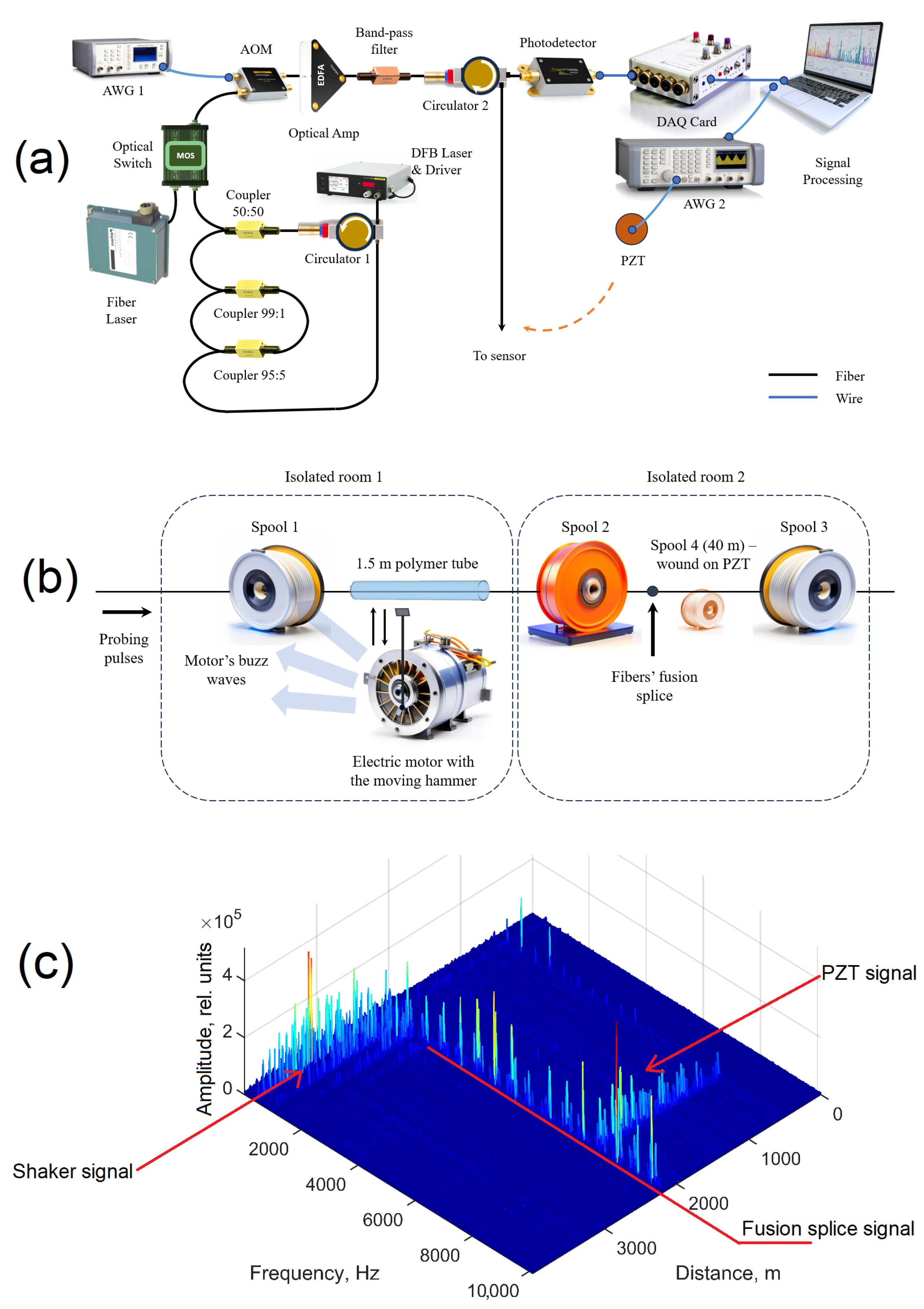
2. Setup and Methods

DAS traces were recorded using a commercial laser with a wavelength of 1552.5 nm and a homemade radiation source based on a telecom laser with a wavelength of 1548.5 nm. The experimental setup previously used in [33] is shown in Figure 1a.

The homemade source bandwidth was significantly reduced, reaching a value of about 6 kHz, using an external fiber resonator and the effect of its frequency capturing by the laser. This mode operation was achieved with two polarization-maintaining fiber splitters and a circulator. The splitters formed an annular fiber filter, and the circulator closed the laser output to itself through a 3.75 m long fiber-optic resonator. The bandwidth of the commercial DAS laser—Koheras Adjustik, NKT Photonics—was 100 Hz. A sensing element made of 4 km SMF-28 optical fiber was interrogated by rectangular pulses with a power of about 100 mW and 100 ns duration, formed by an acousto-optic modulator, EDFA, 2 GHz bandpass filter, and each of the investigated radiation sources in turn. The sensing element impacts were performed utilizing a shaker through 1.5 m of a plastic tube at a distance of approximately 3400 m, with a frequency of 500 Hz and a piezoelectric transducer (PZT) at a distance of about 1800 m, with the frequency of 8000 Hz.

The studied optical fiber was divided into three spools (Figure 1b). The fiber on the Spool 1, as well as its separate fragment, which was placed in a plastic tube 1.5 m long, were located in the acoustically isolated room 1. The PEACO-GDK125 DC motor (Peaco Support, Ltd., Shenzhen, China) was also located there. A piston mechanism was attached to the shaft of its rotor, driving a small hammer. The hammer head moved reciprocally, perpendicular to the axis of symmetry of the plastic tube and the optical fiber located in it. At the highest point of the movement, the hammer struck the plastic tube. The fundamental tone of the hammer strokes had a frequency of 500 Hz, while the noise of the motor had a much wider range, also due to frequencies above the fundamental tone. These sound waves affected all objects in the isolated room 1, including Spool 1. The remaining spools were placed in the isolated room 2. The fiber output of Spool 2 was fusion-spliced to the fiber tip of Spool 3 using a Fujikura 80S arc welder. The first 40 m of the Spool 3 fiber was wound onto a piezoelectric ceramic transducer (PZT) producing an 8 kHz frequency vibration (Spool 4). Thus, two events should be distinguishable on the trace: a pointwise event (in isolated room 2) and a combined one—a pointwise event together with a distributed one (in isolated room 1). The fusion splice location is also viewed as a pointwise event. At the same time, practice has shown that connections between fibers of almost any type show phantom peaks at frequencies that, in fact, are not present in the signal. A set of such frequencies can be seen in the middle of a trace or heatmap. The acoustic vibrations emitted in these two isolated rooms do not mix, which is also visible on heat maps. The variation in the intensity of vibrations along the length of the fiber on Spool 1 can be explained by the fact that one side of the spool is closer to the sound source. It is rather difficult to reliably determine the period of these variations from the heat map, since the line was probed with a pulse whose duration was much greater than the circumference of the spool neck.

As expected, the commercial DAS laser provided the higher SNR (Figure 2,

Table 1. Comparison of the studied algorithms application results.

Laser Type	Event Frequency, kHz	SNR, dB
		No Filtering	MA-MD	AFDA	MA-MD and AFDA
Commercial	0.5	18.8	27.3	22.5	29.2
	8	19.6	19.6	23.3	23.4
Homemade	0.5	15.7	25.0	19.3	26.5
	8	17.9	19.2	21.4	22.8

). The DAQ card sampling rate was 200 MHz. Thus, one period between the pulses was sampled by 8000 points, ensuring that about 25,000 DAS traces could be recorded each second.

The obtained data were then structured as a time series for each recorded point of the optical fiber (as the dependence of the point amplitude on time). Each time series consisted of about 900 points. The data in the time domain were subjected to a fast Fourier transform, and eventually, the data were presented either as three-dimensional surfaces or as so-called “heat maps”. The color and height of the peaks reflected the event (noise or useful signal) amplitude, while the remaining two dimensions reflected its frequency and disposition along the fiber. Next, heat maps or their individual cross sections were processed using the algorithms or their combinations, which are described in the paper below.

2.1. Moving Averaging–Moving Differential

The moving averaging–moving differential (MA-MD) technique has proven itself in time series processing and economics. In addition, attempts have repeatedly been made to process DAS data with it [39]. This method allows one to eliminate the small fluctuations of values and to highlight more significant trends with relatively easy implementation, low computational costs, and acceptable computation time. Another common technology for denoising and classifying DAS events is the neural network. However, this requires significant information and computational resources, at least during the stage of training. In a sense, the MA-MD algorithm can be represented as a bandpass filter, where the set of amplified and suppressed frequencies is determined by the window size of each of the two constituents that make up the method. As a rule, each frequency band requires its own window size for the best gain.

In addition, it was found that the most common DAS implementation of the MA-MD method involves the application of both components in a time domain [39]. This generates a relationship between the quality of the received data, estimated by SNR, and the window size of the constituent parts of the technique—moving averaging and moving differential, respectively.

The following equation can be used to calculate an approximately suitable MD window size:

$${}_{w_{MD}=\left(2k+1\right)\mathrm{floor}\left(\frac{{\nu }_s}{2\nu }\right),}$$

(1)

where k is an integer from 0 to ∞; floor() returns an integer part of a number; ${\nu }_s$ is the sensor sampling frequency (i.e., the number of the traces recorded per second); and $\nu$ is the center frequency of the band in which the presence of a useful signal is expected.

In this case, the MA window size can be taken to be approximately equal to the calculated MD window size. Thus, for noise reduction by the MA-MD method, a window size of 25 counts is suitable for the frequency range of 500 Hz and 1–2 counts are suitable for 8000 Hz band. Some frequency bands (multiples) may feature a window size that provides qualities of processing which are not at the maximum for each, but satisfactory for both of them.

It was decided to test these hypotheses in practice. The test utilized the data acquired from the commercial laser. The following formula was applied to its time domain:

$$d{s}_1^{(w_{MA},w_{MD})}=\frac{1}{w_{MA}}\left({\displaystyle \sum _{i=1+w_{MD}}^{w_{MA}+w_{MD}}{s}_i}-{\displaystyle \sum _{i=1}^{w_{MA}}{s}_i}\right),$$

(2)

where $d{s}_1^{(w_{MA},w_{MD})}$ is the first processed signal level value, $w_{MA}$ is the MA window size, $w_{MD}$ is the MD window size, and $s_i$ is the i-th signal level value.

The obtained results are presented in Figure 3. It can be seen that they are in fairly good agreement with the formula. For the 500 Hz event, the maximum SNR fell on the MA and MD window size values of 23 and 20 or 19 and 24 counts, respectively. And for the 8000 Hz event, they fell on 7 and 1. Fortunately, the latter window sizes also provide the sufficient SNR for the 500 Hz frequency band.

In [39], it is also stated that the window sizes are completely interchangeable, and it is possible to calculate only half of this matrix (Figure 3a,b) to determine the SNR distribution by the MA-MD window sizes in a specific frequency range. However, practice has shown that this is true, with some error. In those frequency regions for which the optimal MD window size is relatively large, the symmetry can, indeed, be observed, with a slight deviation (the line of symmetry passes through the points (11; 10) and (33; 32)). Apparently, the same shift does not allow one to fully see the symmetry for the 8 kHz band, since one of the areas of optimal window sizes goes beyond the allowable values (Figure 3b, top). Nevertheless, in each case, in order to obtain a good SNR increase, one can calculate the MD window size based on Equation (1) and use it to select the most appropriate MA window size.

An obvious disadvantage of the algorithm is the partial data loss, which takes place at the end of the processed time series. The value of this loss depends on the sum of the MA and MD window sizes.

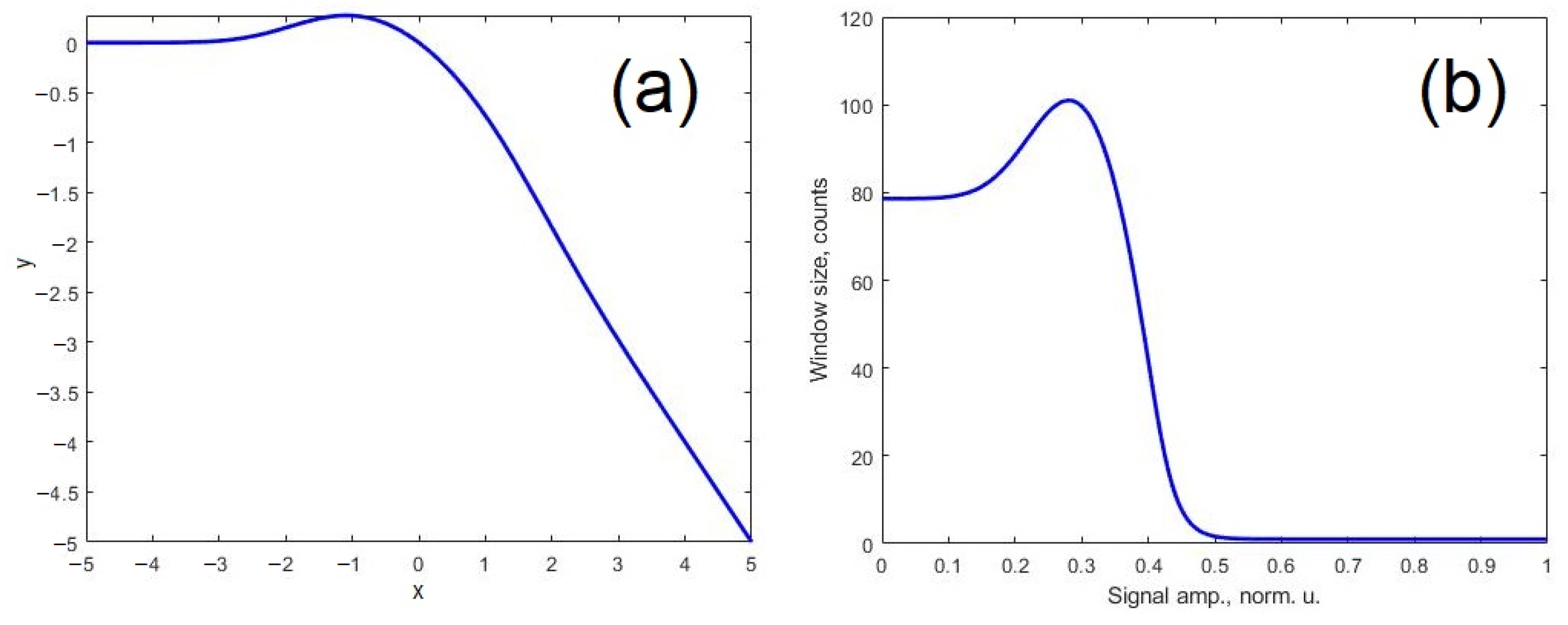
2.2. FDDA Refinement

When the MA-MD pre-processing stage was completed, it became necessary to use the refined version of the FDDA—the frequency domain dynamic averaging algorithm. Its previous implementation assumed that the moving window size was inversely proportional (linearly) to the normalized signal intensity. This led to the realization that, occasionally, some signal components could be mistakenly interpreted as noise and suppressed, and in other cases, on the contrary, some unwanted noise peaks could be identified as useful signals and amplified. It is obvious that the dependence of the moving window size on the signal magnitude needs to be made more sensitive.

Considering the case in which the useful signal is represented by single-frequency components or their combinations, the signal in the spectrum can be divided into three groups according to the intensity normalized to 1:

(1)

Intensities within I₁ and I₂ (assuming that I₁ = 0; I₂ = 0.2). This region contains the noise of the photodetector. If it is averaged with the maximal window size, then its influence is practically zeroed. However, this will lead to an increase in the number of mathematical operations and a decrease in the algorithm speed. It will also blur the boundaries of neighboring (possibly useful) components of the spectrum. Thus, for these intensity components, it is preferable to set the moving window size to about 80% of the maximal allowable one ($w_{\max }$).

(2)

Intensities within I₂ and I₃ (I₂ = 0.2; I₃ = 0.4). Another type of unwanted component may appear in this area: various phantom peaks. The practice of operating inexpensive laser sources has shown that they appear quite often. Sometimes they are electrical in nature and pass through the entire signal in time, frequency, or spatial domains. Since the proposed algorithm will operate in 2D mode, it may help to solve this problem. It is assumed reasonable to use the maximal window size for this intensity region.

(3)

Intensities within I₃ and I₄ (I₃ = 0.4; I₄ = 1). Obviously, this signal contains the main useful part. Such frequency components should not be smoothed across the spectrum, so the averaging window size should be minimal (ideally zero).

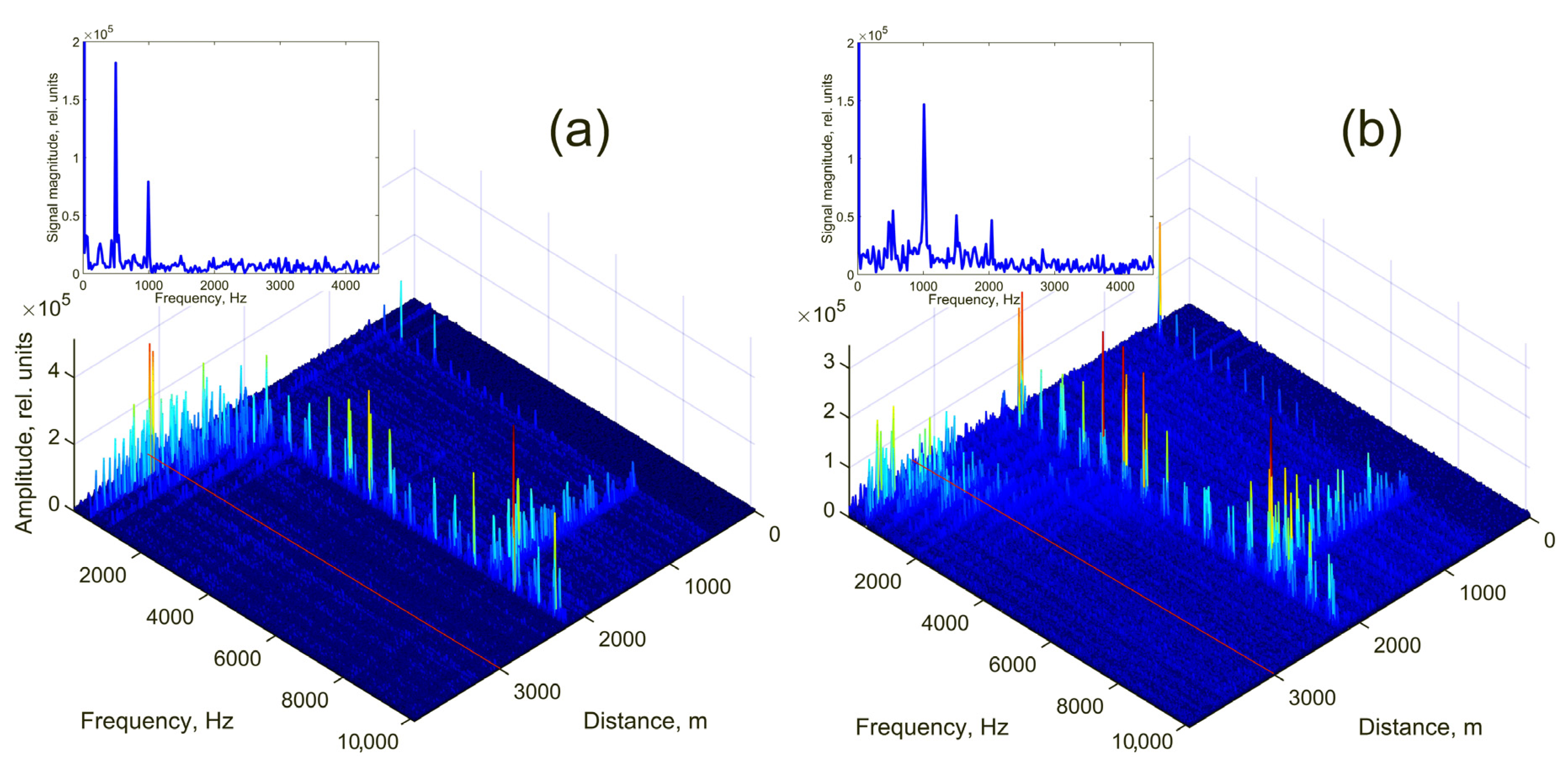
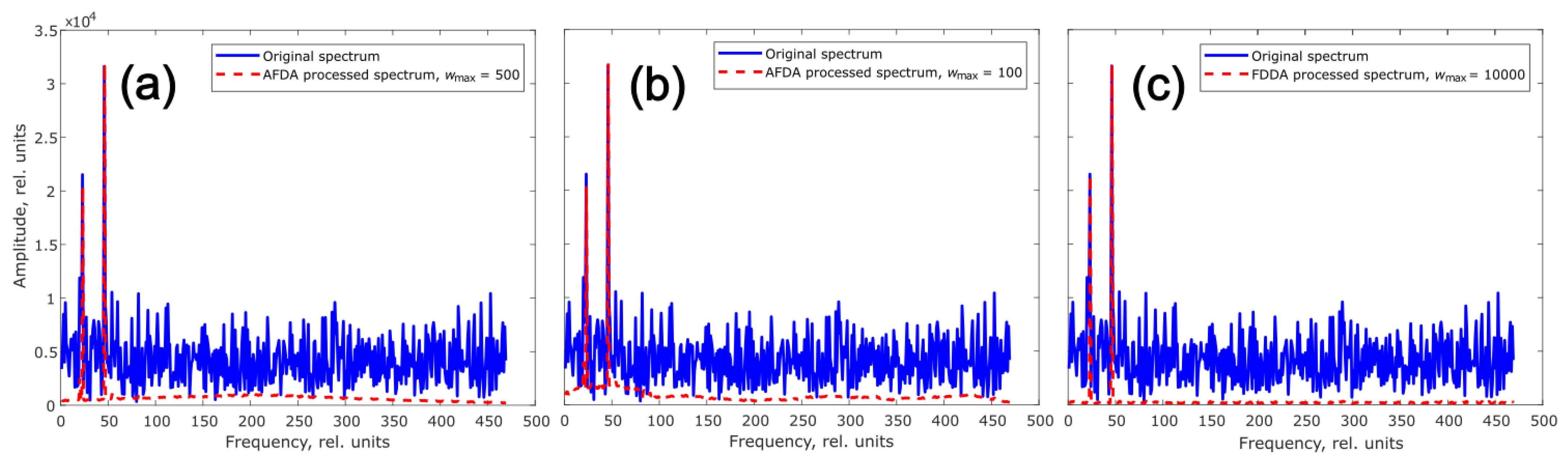
It may seem that different types of noise can be combined into one category, but we have classified them as categories 2 and 3 intentionally. Our solution can be explained as follows. First, noises of different natures require different averaging window sizes. Therefore, this implies dividing the filter operation function into several areas. Secondly, the function should be able to adapt flexibly to various types of experimental data. More areas in a function provide more adjustment options. Of course, characterizing noises solely by their amplitude does not provide a complete description of them. To use this method, it is necessary to have some basic knowledge about the signal that the sensor sends out in each individual case. For example, if a high-quality, stabilized, coherent radiation source is being used, then the likelihood of phantom peaks is much lower. This means that Region 2 of the activation function must be adjusted in such a way that additional peaks are not eliminated, but highlighted. Or if we receive a sensor signal from the first meters of the line, then the signal-to-noise ratio is quite high already in the raw data. This means that some perturbations in Region 1 should not be excluded from the data, since these may be low-intensity useful signals. Thus, the method of filtering noises by their intensity is not applicable to signals of unknown origin.

In case shown above, these three areas are set stepwise, so the processed signal will be significantly distorted. It was discovered that the FDDA algorithm demonstrated earlier operates with a threshold filter (has an abrupt drop in the graph, showing the dependence of the window size on the intensity); therefore, the spectral components are significantly distorted in the region of their substructure.

According to the points 1–3, it is necessary to choose a smooth function for signal processing, in which the values of I₁–I₄ can be easily variable.

Some neuron activation functions in artificial intelligence systems have similar features. The Gaussian Error Linear Unit (GELU) function, for example, has three regions that can be adapted in order to solve this issue by simple inversion (Figure 4a):

$$y=-\frac{x}{2}\left\{1+\mathrm{erf}\left[\frac{x}{\sqrt{2}}\right]\right\}$$

(3)

where $\mathrm{erf}$ is the Gauss error function.

The third area, however, does not fully meet the requirements above, so it is proposed to modify this function by combining it with the exponential one (Figure 4b):

$$\mathrm{windowsize}=A(1-y)w_{\max }+1,$$

(4)

where $y=(3)$ if $x<B$ and

$$y=\frac{1}{1+e^{-3y+C}}$$

(5)

if $x\ge B$.

$$x=\frac{Ds}{s_t}-E$$

(6)

where $s$ is the signal level value in the current point and $s_t$ is the “threshold” signal level value. $A$ = 0.776, $B$ = 0.55585, $C$ = 2.3, $D$ = 9.8, and $E$ = 5.8—these are empirically selected constants.

The parameters of this function can be easily adjusted to various signals obtained using a distributed acoustic sensor.

The original FDDA algorithm featured three variable parameters: $w_{\max },$ s, and the difference between s and the subsequent signal level value. The updated algorithm, AFDA—activation function dynamic averaging—has two variables: $w_{\max }$ and $s_t,$ the latter of which determines the point where the functions are combined. In both cases, the estimated parameter was SNR.

It has been assumed that $w_{\max }$ should not exceed the length of the dataset. The fact is that, in order to avoid data loss and edge effects, full copies of the original dataset were inserted into the areas to the left and right of it. In turn, the areas around this array were filled with zeros. These areas’ sizes were equivalent to half of the maximal window size. In the mentioned side datasets, the influence of the edge effects arising from this did not matter. But when the window size was large (it exceeds the length of the original data array), zero values from the extreme regions overlapped the window during averaging, leading to an attractive-looking image of the processed data: the noise signal became almost zero while the useful signal became significantly highlighted (Figure 5c).

Nevertheless, such a result is implausible, since the original signal typically does not include many values of zero. The result obtained in this case was very close to the operation of a threshold filter that cuts off the signal below a given threshold level. If the useful signal is close to the spectrum edges, a large $w_{\max }$ leads to an influence of this signal on the noise region during averaging and causes various kinds of distortions, for example, an appearance of a “dip” in the location of the processed spectrum (Figure 5a) or an emerging of phantom side peaks. However, the areas to the left and right of the original dataset still needed to be filled with something. In general, the useful signal can be located anywhere, and the noise is somewhat different for different spectra. It is not possible to fill this region with noise samples while retaining an acceptable calculation time. The average signal value of the spectrum is also strongly influenced by the high-amplitude useful signal. For this reason, and also since in many cases (including the studied one), the useful signal in the DAS spectrum is represented by much fewer samples than the noise, it was decided to use the spectrum signal level mode. This mode fills only half the maximum averaging window size in the designated areas. In our case, the mode of the spectrum signal level indicates one of the most frequently occurring values of a signal level in it. Limiting $w_{\max }$ to the length of the original data sample still did not eliminate the spectrum distortion caused by taking into account large values of the useful signal when the window moves over a noise region far from them (Figure 5a).

An experiment regarding iterating over different $w_{\max }$ values when processing the same spectra at constant $s_t$ led to the conclusion that $w_{\max }$ should be approximately equal to the local bandwidth of the useful signal (Figure 5b). In this case, acceptable noise suppression was achieved, and the maximum (middle) of the “pedestal” fell in the middle of the useful signal band.

In this work, we applied the algorithm sequentially to the frequency and to the spatial domain (to the frequency and spatial cross sections in Figure 2). Since the method had 2 variable ($w_{\max }, s_t$) and 1 estimated (SNR) parameter, it was decided to search for the optimal values for two types of the useful signal cross sections using heatmaps (Figure 6a,b).

The optimal value of $w_{\max }$ for the cross section 6c (Figure 6c) was 98 counts, and $s_t$ was 0.51. For cross section 6d (Figure 6d), these values were 180 counts and 0.85, respectively. The obtained results allowed us to draw conclusions not only regarding the existence similarity of optimal values for similar ratios of amplitudes and the local signal bandwidth in the spatial or frequency domain, but also regarding the validity of the previous assumptions. Thus, the useful signal bandwidth in the frequency domain was about 100 rel. units, and in the spatial, about 200. The calculated optimal $w_{\max }$ values turned out to be approximately equal. Therefore, when processing the 2D data (acoustic spectrum distribution over space, Figure 2, for instance) with AFDA, firstly, all of the frequency-domain cross sections were processed with $w_{\max }$ = 100 rel. units, and the spatial ones with $w_{\max }$ = 200 rel. units. It also has been noticed that it is this sequence that results in a slightly better SNR than the opposite.

3. Results

The presented modifications of the FDDA algorithm made it possible to reduce the calculation time by approximately eightfold (

Table 2. Algorithms’ computation time comparison.

Algorithm	Computation Time, s	Spatial Resolution, m
MA-MD	13.1	1
AFDA	24.9	1
FDDA	200.0	100

) and to make the results more plausible by reducing spatial distortions (Figure 7b) inherent to the original technique. In addition, the use of an activation function instead of a threshold algorithm improved the events’ classification quality, showing that the shaker signal was more broadband and distributed in space than the PZT signal (Figure 7).

Data obtained using either the homemade or the commercial laser were processed with the presented implementation of MA-MD or AFDA, both individually and combined. The obtained results are presented in Figure 8. The corresponding SNR values for each case are presented in Table 1. This SNR was calculated for the data sets presented in Figure 8, as follows:

$$\mathrm{SNR}=10{\log }_{10}\left[\frac{s_{\max }}{\left({\displaystyle \sum _{j=1}^k{\displaystyle \sum _{i=1}^n{s}_{i,j}-s_{\max }}}\right)/(k·n-1)}\right]$$

(7)

where $s_{\max }$ is the maximum useful signal level value in the data set; $s_{i,j}$ is the i, jth data set value, k is the data set size in spatial domain, and n is the data set size in the frequency domain.

It can be seen that in all the studied cases, it was the combined use of the MA-MD and AFDA algorithms that led to the greatest increase in SNR. In addition, MA-MD is the most efficient when processing a signal with a frequency of 500 Hz, while AFDA is more efficient when processing a signal with the frequency of 8 kHz. Processing using any of the studied algorithms makes it possible to approximate the SNR of DAS data obtained using the homemade laser to the SNR of data obtained using the commercial laser. For the homemade laser, the most optimal MA and MD windows values for each of the useful signal frequencies turned out to be slightly different from those for the commercial laser. Thus, for the homemade laser and 500 Hz event, the MA and MD window sizes were 14 counts and 20 counts, respectively, or 19 counts and 15 counts. For the 8 kHz event, these values were 1 and 1, respectively. Just as in the first case, matrix symmetry was observed, similar to Figure 3a, as well as interchangeability of the window sizes with a small error. In the second case, the optimal window sizes turned out to be completely interchangeable and equal. This was probably caused by a slight impact frequency shift, which is actually present in the data and has already been stated by our team [33].

4. Discussion

The noise reduction algorithms studied herein and applied to DAS data processing have similar computational times. The use of any of them makes it possible to achieve output DAS data characteristics from the use of a simple and affordable homemade laser similar to those of the commercial laser source. This provides an opportunity to make distributed acoustic monitoring less expensive and, therefore, more accessible.

To prove this statement, an extreme noise data filtering case was considered. Homemade laser-obtained raw data were resampled. Thus, an ADC sampling rate of 1.25 MHz instead of 200 MHz was simulated. Next, a random noise was added to it, and the resulting dataset (Figure 9a) was processed by the AFDA algorithm. The algorithm kept working even in these difficult conditions and provided an SNR increase of 2.6 dB (Figure 9b), which made it possible to distinguish the signal from the noise.

The study results show that the algorithms have different efficiency levels for different event frequencies. Also, some restrictions on the types of processed signals follow from the very nature of these algorithms. In addition, the time spent on post-processing can be quite a critical parameter in some applications. Thus, there is a need to differentiate algorithms according to the types and frequencies of processed events in order to reduce the calculation time and maintain an acceptable quality of the output data. MA-MD is best suited for single signals or far-spaced multiple frequency bands; provided that the event frequency is approximately known in advance, the resulting loss of data portion at the end of each time sequence is not significant, and the frequency band for which SNR is increased, but does not exceed 1/2 of the sensor sampling frequency. AFDA, in turn, is most efficient when processing wide-band signals, as well as single useful signals which are randomly distributed over the entire spectrum or in the presence of multiple harmonics. Its works adequately as long as the useful signal fraction in the data is less than the noise fraction over the total occupied spatial or frequency domain. It does not require information about the expected event frequency, although data on the approximate magnitude and width (in frequency and spatial domains) of the most significant signal components may be needed for the best performance. It is inferior to MA-MD when processing single signals from a known frequency band in the low-frequency region (relative to the sampling frequency). However, it is a good complement to MA-MD in cases in which computation time is not the most important parameter. A raw data set consisting of 7,560,000 samples was processed by the MA-MD, AFDA, and FDDA algorithms in turn. In each case, the computation time was recorded to evaluate the computational complexity. The results are presented in Table 2.

The use of AFDA method avoids spatial distortions caused by FDDA’s edge effects. The maximum size of such distortions is half the maximum length of the scanning window. The AFDA method does not provide for edge effects, so the spatial resolution when using it is determined only by the length of the probing pulse and the sampling frequency of the data acquisition card. Thus, for a scanning window length of 200 m, the spatial resolution when using the FDDA method is 100 m, and when using the AFDA method it is 10 m, since the pulse length is 100 ns (Table 2).

The MA-MD computation time, of course, slightly depends on the MA and MD window sizes. Its value, shown in Table 2, was achieved with a window size of 1. If changed to 25, the computation time would become16 s.

Meanwhile, the current MA-MD implementation, which has been repeatedly applied to DAS data, has asymmetrical MA and MD window positions relative to the point under processing. The resulting data loss at the end of the processed time series has already been mentioned. But an important aspect of the feature under discussion is the higher probability of data distortion, since the current value of a point takes into account only the signal values at subsequent points, but not at previous ones. A window that is symmetrical in the area of the point under processing, however, will either result in a loss of data at both ends of the time series or in the problem of filling areas at the beginning and end. In this work, a similar problem was solved for the AFDA algorithm and frequency or time cross sections of DAS data. The upcoming research will, most likely, be aimed at finding a solution to the problem of the MA-MD algorithm. In addition, it should include the calculation of SNR dependence on the frequency of the useful signal provided by the use of each of the algorithms. This will allow for the determination of the most efficient performance range of the MA-MD and AFDA methods. Such an estimate is necessary because, in this work, it was found out that the resulting SNR depended on how the signal frequency correlated with the sampling frequency.

Such cost-effective sensors can also be widely used in biology and agriculture, where there is a need for distributed acoustic monitoring, and suitability of fiber optic DAS for this has already been confirmed [48]. It is important to note that pest registration [49] and the monitoring of the state of beneficial insects [50] or plant crops [51] are associated precisely with the specific tracking of frequency bands in the signal spectrum, and therefore, the results of this work can be very useful.

The described features of the algorithms and their possible applications are summarized in

Table 3. Features and potential applications of the studied algorithms.

Algorithm	Most Suitable Event Type	Limitations	Potential Applications
MA-MD	Pointwise	Requires event frequency information; partial data loss; high frequencies reduce efficiency	Railway monitoring, pest registration, flow metering
AFDA	Distributed; high-frequency	The signal fraction should be less than noise fraction; may require information on signal characteristics	Flaw detection, perimeter security, bee and plant monitoring

.

Another interesting direction of future work may be the application of the developed method in the time domain. In this case, the time domain refers to the intensity of the acoustic vibration as a function of time at a single point in the optical fiber. In sound engineering, non-linear processing is widely applied to such data. For example, when there is a need to make the sound denser, by compensating the changing distance from the sound source (singer) to the sensor (microphone), a compression procedure is applied. When the task is to make the dynamics of intensity variation more noticeable, the reverse procedure is used—expanding. In classical sound engineering, these processing methods operate on the principle of raising intensity values to a power, and the exponent determines whether the signal becomes dynamically more diverse or not. Processing an audio signal using an inverted activation function is somewhat similar to expanding, since loud sounds will become even louder, and quiet ones even quieter. In this case, quiet sounds will lose their readability due to averaging over time (an effect similar to delay and reverb). It is expected that this will be useful for isolating a voice from extraneous noise (for example, other voices) for the purpose of further speech recognition.

5. Conclusions

In this work, we describe a new approach for the non-linear 2D processing of data from a distributed acoustic sensor implemented in both the time and frequency domains. when using an inexpensive radiation source, it allows various types of noise to be excluded, leading to a maximum increase in the signal-to-noise ratio of the received data. Basic information regarding the supposed nature of noises allows us to rank them by intensity (rather than by frequency, as is usually the case) and to adjust filtering parameters for each type of noise. Through the refinement of simple and undemanding DAS noise reduction algorithms, an improvement in their performance was achieved: the processed data SNR was increased, and spatial distortions and operating time were reduced (compared to the FDDA technique). Thus, the dynamic averaging algorithm began to work up to eight times faster, providing an increase in SNR of 3.7 dB on its own and in combination with MA-MD by 10.8 dB. The differentiation of algorithms by types of processed actions has been proposed. All of this makes it possible to reduce the DAS cost and increase accessibility, hence expanding the scope of their application.

The SNR enhancement was achieved due to a new method, which involves using the inverted activation function to determine the best averaging parameters. In fact, the key varying calculation options are the parameters of this function, as well as the window sizes when calculating the moving differential and moving averaging. In the future, the selection of these parameters can be entrusted to artificial intelligence. After training the system, this will not require serious additional computing resources. We expect that the proposed combined application of algorithms and artificial intelligence methods will expand the possibilities surrounding distributed acoustic sensor utilization for the registration of voice commands [52,53,54] and their origin localization in smart home systems, smart production [55,56,57], and other Internet of Things applications [58].

References

1. Karapanagiotis, C.; Krebber, K. Machine Learning Approaches in Brillouin Distributed Fiber Optic Sensors. Sensors 2023, 23, 6187. [Google Scholar] [CrossRef]
2. Fomiryakov, E.A.; Bengalskii, D.M.; Kharasov, D.R.; Nanii, O.E.; Nikitin, S.P.; Treshchikov, V.N. Influence of Laser Phase Noise on the Operation of a Coherent Reflectometer Using Fiber with Arrays of Artificial Reflectors. Optoelectron. Instrum. Data Process. 2023, 59, 77–99. [Google Scholar] [CrossRef]
3. Alekhin, I.N.; Dashkov, M.V.; Nikulina, T.G. Application of the polarization reflectometry for estimating the distribution of mechanical stress in optical fiber. In Proceedings of the Optical Technologies for Telecommunications 2018, Ufa, Russia, 24 June 2019; Volume 11146, pp. 460–467. [Google Scholar]
4. Taranov, M.A.; Gorshkov, B.G.; Alekseev, A.E. Achievement of an 85 km distance range of strain (temperature) measurements using low-coherence Rayleigh reflectometry. Instrum. Exp. Technol. 2020, 63, 527–531. [Google Scholar] [CrossRef]
5. Kharasov, D.R.; Bengalskii, D.M.; Vyatkin, M.Y.; Nanii, O.E.E.; Fomiryakov, E.A.; Nikitin, S.P.; Popov, S.M.; Chamorovsky, Y.K.; Treshchikov, V.N. Extending the operation range of a phase-sensitive optical time-domain reflectometer by using fibre with chirped Bragg gratings. Quantum Electron. 2020, 50, 510. [Google Scholar] [CrossRef]
6. Lin, Z.; Zhao, Z.; Liu, D.; Tang, M. Ultra-high Frequency Vibration Measurement using Fading Suppressed Coherent φ-OTDR with Randomized Sampling. In Proceedings of the 2022 Conference on Lasers and Electro-Optics (CLEO), San Jose, CA, USA, 15–20 May 2022; pp. 1–2. [Google Scholar]
7. Gorshkov, B.G.; Alekseev, A.E.; Simikin, D.E.; Taranov, M.A.; Zhukov, K.M.; Potapov, V.T. A Cost-Effective Distributed Acoustic Sensor for Engineering Geology. Sensors 2022, 22, 9482. [Google Scholar] [CrossRef] [PubMed]
8. Hartog, A.; Liokumovich, L.B.; Ushakov, N.A.; Kotov, O.I.; Dean, T.; Cuny, T.; Constantinou, A. The use of multi-frequency acquisition to significantly improve the quality of fibre-optic distributed vibration sensing. In Proceedings of the 78th EAGE Conference and Exhibition 2016, Vienna, Austria, 30 May–2 June 2016; pp. 1–5. [Google Scholar]
9. Zhirnov, A.A.; Choban, T.V.; Stepanov, K.V.; Koshelev, K.I.; Chernutsky, A.O.; Pnev, A.B.; Karasik, V.E. Distributed acoustic sensor using a double sagnac interferometer based on wavelength division multiplexing. Sensors 2022, 22, 2772. [Google Scholar] [CrossRef] [PubMed]
10. Zhirnov, A.A.; Chesnokov, G.Y.; Stepanov, K.V.; Gritsenko, T.V.; Khan, R.I.; Koshelev, K.I.; Chernutsky, A.O.; Svelto, C.; Pnev, A.B.; Valba, O.V. Fiber-Optic Telecommunication Network Wells Monitoring by Phase-Sensitive Optical Time-Domain Reflectometer with Disturbance Recognition. Sensors 2023, 23, 4978. [Google Scholar] [CrossRef]
11. Wang, Y.; Xu, R.; Deng, Z.; Liang, Y.; Jiang, J.; Wang, Z. High-Performance Distributed Acoustic Sensing with Coherent Detection. In Proceedings of the 2022 IEEE 10th International Conference on Information, Communication and Networks (ICICN), Zhangye, China, 23–24 August 2022; pp. 485–488. [Google Scholar]
12. Yablochkin, K.A.; Dashkov, M.V. Study of the vibration detection using few-mode optical fiber. In Proceedings of the XVII International Scientific and Technical Conference “Optical Technologies for Telecommunications”, Kazan, Russia, 22 May 2020; Volume 11516, pp. 236–242. [Google Scholar]
13. Wang, S.; Liu, F.; Liu, B. Semi-supervised deep learning in high-speed railway track detection based on distributed fiber acoustic sensing. Sensors 2022, 22, 413. [Google Scholar] [CrossRef]
14. Egan, D.A.; James, S.W.; Tatam, R.P. A polarization-based optical fibre vibrometer. Meas. Sci. Technol. 1997, 8, 343. [Google Scholar] [CrossRef]
15. Titov, A.; Fan, Y.; Jin, G.; Tura, A.; Kutun, K.; Miskimins, J. Experimental investigation of distributed acoustic fiber-optic sensing in production logging: Thermal slug tracking and multiphase flow characterization. In Proceedings of the SPE Annual Technical Conference and Exhibition, New Orleans, LA, USA, 5–8 October 2020; p. D041S044R006. [Google Scholar]
16. Peng, Z.; Jian, J.; Wen, H.; Gribok, A.; Wang, M.; Liu, H.; Huang, S.; Mao, Z.-H.; Chen, K.P. Distributed fiber sensor and machine learning data analytics for pipeline protection against extrinsic intrusions and intrinsic corrosions. Opt. Express 2020, 28, 27277–27292. [Google Scholar] [CrossRef]
17. Matveenko, V.; Kosheleva, N.; Serovaev, G.; Fedorov, A. Measurement of Gradient Strain Fields with Fiber-Optic Sensors. Sensors 2022, 23, 410. [Google Scholar] [CrossRef] [PubMed]
18. Gao, L.; Qian, J.; Han, C.; Qin, S.; Feng, K. Experimental Study of Deformation Measurement of Bored Pile Using OFDR and BOTDR Joint Optical Fiber Sensing Technology. Sustainability 2022, 14, 16557. [Google Scholar] [CrossRef]
19. Abedin, S.; Biondi, A.M.; Wu, R.; Cao, L.; Wang, X. Structural health monitoring using a new type of distributed fiber optic smart textiles in combination with optical frequency domain reflectometry (OFDR): Taking a pedestrian bridge as case study. Sensors 2023, 23, 1591. [Google Scholar] [CrossRef]
20. Murayama, H.; Kageyama, K.; Uzawa, K.; Igawa, H.; Omichi, K.; Machijima, Y. Distributed fiber-optic sensing system with OFDR and its applications to structural health monitoring. In Proceedings of the Second International Conference on Smart Materials and Nanotechnology in Engineering, Weihai, China, 20 October 2009; Volume 7493, pp. 118–125. [Google Scholar]
21. Stepanov, K.V.; Zhirnov, A.A.; Sazonkin, S.G.; Pnev, A.B.; Bobrov, A.N.; Yagodnikov, D.A. Non-invasive acoustic monitoring of gas turbine units by fiber optic sensors. Sensors 2022, 22, 4781. [Google Scholar] [CrossRef] [PubMed]
22. Bakhoum, E.G.; Zhang, C.; Cheng, M.H. Real time measurement of airplane flutter via distributed acoustic sensing. Aerospace 2020, 7, 125. [Google Scholar] [CrossRef]
23. Nordon, A.; Waddell, R.J.; Bellamy, L.J.; Gachagan, A.; McNab, D.; Littlejohn, D.; Hayward, G. Monitoring of a heterogeneous reaction by acoustic emission. Analyst 2004, 129, 463–467. [Google Scholar] [CrossRef]
24. Chen, B.; Wang, Y.; Yan, Z. Use of acoustic emission and pattern recognition for crack detection of a large carbide anvil. Sensors 2018, 18, 386. [Google Scholar] [CrossRef]
25. Zhang, L.; Ji, H.; Liu, L.; Zhao, J. Time–frequency domain characteristics of acoustic emission signals and critical fracture precursor signals in the deep granite deformation process. Appl. Sci. 2021, 11, 8236. [Google Scholar] [CrossRef]
26. Haile, M.A.; Bordick, N.E.; Riddick, J.C. Distributed acoustic emission sensing for large complex air structures. Struct. Health Monit. 2018, 17, 624–634. [Google Scholar] [CrossRef]
27. Mendoza, E.; Prohaska, J.; Kempen, C.; Esterkin, Y.; Sun, S.; Krishnaswamy, S. Distributed fiber optic acoustic emission sensor (FAESense™) system for condition based maintenance of advanced structures. In Proceedings of the Optical Sensors, Rio Grande, PR, USA, 14–17 July 2013; p. SM4C-4. [Google Scholar]
28. Liang, S.; Zhang, C.; Lin, W.; Li, L.; Li, C.; Feng, X.; Lin, B. Fiber-optic intrinsic distributed acoustic emission sensor for large structure health monitoring. Opt. Lett. 2009, 34, 1858–1860. [Google Scholar] [CrossRef]
29. Marcon, L.; Galtarossa, A.; Palmieri, L. High-frequency high-resolution distributed acoustic sensing by optical frequency domain reflectometry. Opt. Express 2019, 27, 13923–13933. [Google Scholar] [CrossRef] [PubMed]
30. Paitz, P.; Edme, P.; Schmelzbach, C.; Doetsch, J.; Gräff, D.; Walter, F.; Lindsey, N.; Chalari, A.; Fichtner, A. Distributed Acoustic Sensing from mHz to kHz: Empirical Investigations of DAS instrument response. Copernic. Meet. 2020, EGU2020, 7343. [Google Scholar]
31. Tang, J.; Cai, L.; Li, C.; Yang, M.; Guo, H.; Gan, W. Distributed acoustic sensors with wide frequency response based on UWFBG array utilizing dual-pulse detection. Opt. Fiber Technol. 2021, 61, 102452. [Google Scholar] [CrossRef]
32. Iida, D.; Toge, K.; Manabe, T. High-frequency distributed acoustic sensing faster than repetition limit with frequency-multiplexed phase-OTDR. In Proceedings of the Optical Fiber Communication Conference, Anaheim, CA, USA, 20–24 March 2016; p. M2D-6. [Google Scholar]
33. Escobedo, J.B.; Jason, J.; López-Mercado, C.A.; Spirin, V.V.; Wuilpart, M.; Mégret, P.; Korobko, D.A.; Zolotovskiy, I.O.; Fotiadi, A.A. Distributed measurements of vibration frequency using phase-OTDR with a DFB laser self-stabilized through PM fiber ring cavity. Results Phys. 2019, 12, 1840–1842. [Google Scholar] [CrossRef]
34. Popov, S.M.; Butov, O.V.; Bazakutsa, A.P.; Vyatkin, M.Y.; Chamorovskii, Y.K.; Fotiadi, A.A. Random lasing in a short Er-doped artificial Rayleigh fiber. Results Phys. 2020, 16, 102868. [Google Scholar] [CrossRef]
35. Bublin, M. Event detection for distributed acoustic sensing: Combining knowledge-based, classical machine learning, and deep learning approaches. Sensors 2021, 21, 7527. [Google Scholar] [CrossRef]
36. Shiloh, L.; Eyal, A.; Giryes, R. Efficient processing of distributed acoustic sensing data using a deep learning approach. J. Light. Technol. 2019, 37, 4755–4762. [Google Scholar] [CrossRef]
37. Shi, Y.; Wang, Y.; Zhao, L.; Fan, Z. An event recognition method for Φ-OTDR sensing system based on deep learning. Sensors 2019, 19, 3421. [Google Scholar] [CrossRef]
38. Turov, A.T.; Konstantinov, Y.A.; Barkov, F.L.; Korobko, D.A.; Zolotovskii, I.O.; Lopez-Mercado, C.A.; Fotiadi, A.A. Enhancing the Distributed Acoustic Sensors’(DAS) Performance by the Simple Noise Reduction Algorithms Sequential Application. Algorithms 2023, 16, 217. [Google Scholar] [CrossRef]
39. Zhu, X.; Zhao, S.; Li, X.; Zhang, R.; Kong, M. Optimization of the moving averaging–moving differential algorithm for Φ-OTDR. Appl. Opt. 2022, 61, 5633–5639. [Google Scholar] [CrossRef]
40. Liang, Y.; Wang, Z.; Lin, S.; Wang, Y.; Jiang, J.; Qiu, Z.; Liu, C.; Rao, Y. Optical-pulse-coding phase-sensitive OTDR with mismatched filtering. Sci. China Inf. Sci. 2022, 65, 192303. [Google Scholar] [CrossRef]
41. Poddubrovskii, N.R.; Lobach, I.A.; Kablukov, S.I. Signal Processing in Optical Frequency Domain Reflectometry Systems Based on Self-Sweeping Fiber Laser with Continuous-Wave Intensity Dynamics. Algorithms 2023, 16, 260. [Google Scholar] [CrossRef]
42. Lopez-Mercado, C.A.; Korobko, D.A.; Zolotovskii, I.O.; Fotiadi, A.A. Application of Dual-Frequency Self-Injection Locked DFB Laser for Brillouin Optical Time Domain Analysis. Sensors 2021, 21, 6859. [Google Scholar] [CrossRef] [PubMed]
43. Barkov, F.L.; Krivosheev, A.I.; Konstantinov, Y.A.; Davydov, A.R. A Refinement of Backward Correlation Technique for Precise Brillouin Frequency Shift Extraction. Fibers 2023, 11, 51. [Google Scholar] [CrossRef]
44. Krivosheev, A.I.; Konstantinov, Y.A.; Krishtop, V.V.; Turov, A.T.; Barkov, F.L.; Zhirnov, A.A.; Garin, E.O.; Pnev, A.B. A Neural Network Method for The BFS Extraction. In Proceedings of the 2022 International Conference Laser Optics (ICLO), St. Petersburg, Russia, 20–24 June 2022. [Google Scholar]
45. Qian, X.; Wang, Z.; Wang, S.; Xue, N.; Sun, W.; Zhang, L.; Zhang, B.; Rao, Y. 157 km BOTDA with pulse coding and image processing. In Proceedings of the Sixth European Workshop on Optical Fibre Sensors, Limerick, Ireland, 31 May–3 June 2016; Volume 9916, pp. 395–398. [Google Scholar]
46. Soto, M.A.; Ramírez, J.A.; Thévenaz, L. Optimizing image denoising for long-range Brillouin distributed fiber sensing. J. Light. Technol. 2017, 36, 1168–1177. [Google Scholar] [CrossRef]
47. Hu, Y.; Shang, Q. Performance enhancement of BOTDA based on the image super-resolution reconstruction. IEEE Sens. J. 2021, 22, 3397–3404. [Google Scholar] [CrossRef]
48. Ashry, I.; Mao, Y.; Al-Fehaid, Y.; Al-Shawaf, A.; Al-Bagshi, M.; Al-Brahim, S.; Ng, T.K.; Ooi, B.S. Early detection of red palm weevil using distributed optical sensor. Sci. Rep. 2020, 10, 3155. [Google Scholar] [CrossRef]
49. Ashry, I.; Wang, B.; Mao, Y.; Sait, M.; Guo, Y.; Al-Fehaid, Y.; Al-Shawaf, A.; Ng, T.K.; Ooi, B.S. CNN–Aided Optical Fiber Distributed Acoustic Sensing for Early Detection of Red Palm Weevil: A Field Experiment. Sensors 2022, 22, 6491. [Google Scholar] [CrossRef]
50. Abdollahi, M.; Giovenazzo, P.; Falk, T.H. Automated beehive acoustics monitoring: A comprehensive review of the literature and recommendations for future work. Appl. Sci. 2022, 12, 3920. [Google Scholar] [CrossRef]
51. Khait, I.; Lewin-Epstein, O.; Sharon, R.; Saban, K.; Goldstein, R.; Anikster, Y.; Zeron, Y.; Agassy, C.; Nizan, S.; Sharabi, G.; et al. Sounds emitted by plants under stress are airborne and informative. Cell 2023, 186, 1328–1336. [Google Scholar] [CrossRef]
52. Shang, Y.; Yang, J.; Chen, W.; Yi, J.; Sun, M.; Du, Y.; Huang, S.; Zhao, W.; Qu, S.; Wang, W.; et al. Speech signal enhancement based on deep learning in distributed acoustic sensing. Opt. Express 2023, 31, 4067–4079. [Google Scholar] [CrossRef]
53. Xu, R.; Sun, J.; Wang, Y.; Zhang, S.; Zhong, W.; Wang, Z. Speech Enhancement Based on Array-processing-assisted Distributed Fiber Acoustic Sensing. IEEE Sens. J. 2023, 23, 11656–11661. [Google Scholar] [CrossRef]
54. Tomboza, W.; Guerrier, S.; Awwad, E.; Dorize, C. High sensitivity differential phase OTDR for acoustic signals detection. IEEE Photonics Technol. Lett. 2021, 33, 645–648. [Google Scholar] [CrossRef]
55. Iliev, Y.; Ilieva, G. A Framework for Smart Home System with Voice Control Using NLP Methods. Electronics 2022, 12, 116. [Google Scholar] [CrossRef]
56. Froiz-Míguez, I.; Fraga-Lamas, P.; Fernández-Caramés, T.M. Design, Implementation and Practical Evaluation of a Voice Recognition Based IoT Home Automation System for Low-Resource Languages and Resource-Constrained Edge IoT Devices: A System for Galician and Mobile Opportunistic Scenarios. IEEE Access 2023, 11, 63623–63649. [Google Scholar] [CrossRef]
57. Torad, M.A.; Bouallegue, B.; Ahmed, A.M. A voice controlled smart home automation system using artificial intelligent and internet of things. TELKOMNIKA 2022, 20, 808–816. [Google Scholar] [CrossRef]
58. Sangaiah, A.K.; Javadpour, A.; Ja’fari, F.; Zavieh, H.; Khaniabadi, S.M. SALA-IoT: Self-reduced internet of things with learning automaton sleep scheduling algorithm. IEEE Sens. J. 2023. [Google Scholar] [CrossRef]
Figure 1. (a) The DAS traces’ acquisition setup, applying the commercial and the homemade laser. AWG—arbitrary waveform generator; DFB—distributed feedback; DAQ—data acquisition system; MOS—manual optical switch. (b) The schematics of the experiment and fiber optic sensing element. (c) The phenomena that took place and were detected.
Algorithms 16 00440 g001
Figure 2. (a) Data obtained with the commercial laser; (b) data obtained with the homemade laser; inserts represent spectra (frequency domain cross sections) at a distance of 3000 m (red lines).
Algorithms 16 00440 g002
Figure 3. SNR dependence on the MA and MD window size for 500 Hz (a) and 8000 Hz (b) events; the commercial laser obtained DAS data, processed using MA-MD technique with MA and MD window sizes (c) 19 and 24 counts, respectively; (d) 7 and 1 counts, respectively.
Algorithms 16 00440 g003
Figure 4. (a) Inverse GELU function; (b) form of the activation function for the maximum averaging window size of w max = 100 counts, and threshold-normalized signal level value of s t = 0.6.
Algorithms 16 00440 g004
Figure 5. Original and AFDA-processed spectra at different w max , s t = 0.5; (a) w max = 500; (b) w max = 100 counts. (c) Original and FDDA-processed spectrum at w max = 10,000 counts.
Algorithms 16 00440 g005
Figure 6. SNR dependence on s t and w max . (a): SNR dependence when processing the frequency cross section (c); (b) SNR dependence when processing the spatial cross section (d).
Algorithms 16 00440 g006
Figure 7. (a) Original data set; (b) data processed by the FDDA algorithm, with red arrows indicating excessive spatial distortions; (c) data processed by the AFDA algorithm.
Algorithms 16 00440 g007
Figure 8. Data (af) obtained using the commercial laser (CL); (gl) obtained using the homemade laser—HL; (a,g) without filtering; (b,h) filtered with AFDA; (c,e,i,k) filtered with MA-MD; (d,f,j,l) filtered with MA-MD and AFDA. (c,d,i,j) MA-MD was adjusted to a 500 Hz frequency band; (e,f,k,l) MA-MD was adjusted to an 8 kHz frequency band.
Algorithms 16 00440 g008
Figure 9. Extremely noisy data filtering with AFDA. (a) Original noisy data set, SNR = 7.3 dB; (b) data processed by the AFDA algorithm, SNR = 9.9 dB.
Algorithms 16 00440 g009