Optimal Integrated Single-Framework Algorithm for the Multi-Level School Bus Network Problem

Abstract

In many states in the United States, school bus fleets are assigned to serve students sequentially at three levels—high school, middle school, and elementary school; however, in past studies, each of these stages in the problem was considered separately. This study introduces a novel integrated school bus problem that considers the sequential operation of fleets for all three levels in a unified framework. An example of a hypothetical network was developed and tested to demonstrate the developed algorithm. The algorithm successfully handled the integration of school buses’ optimal route generation while meeting all constraints. The results showed that the routings with the integrated single-framework algorithm can reduce the total costs by 4.5% to 12.4% compared to the routings with the separated level algorithm. Also, it showed that the total costs of the integrated routing framework for different morning and afternoon time windows are 8.28% less than the same routings (identically reversed) for the morning and afternoon time windows.

1. Introduction

The school bus system is an essential transportation mode for public school students in most states in the U.S. Since each system covers quite a wide area, contains multiple depots for the buses, and serves many high schools, middle schools, and elementary schools, optimizing the operation is a complicated problem. Among the many aspects of school bus operations, one of the fundamental problems is optimizing the school bus routings. Optimal routing of school buses not only minimizes operating costs but also improves the level of service for students by minimizing their in-vehicle travel times. However, as mentioned, school bus routing is a complex problem because, in most cases, a bus leaves a depot and covers a high school, a middle school, and an elementary school in one trip.

Optimizing school bus routing is crucial for ensuring efficient resource allocation and cost savings for educational institutions. Additionally, effective routing enhances student wellness, reduces environmental impact, and improves overall logistical efficiency. The benefits of routing optimization for transit service operators have been broadly considered in past studies [1,2,3], and, similarly, optimization of school bus routes not only benefits the service provider by decreasing the route length and fleet size but also can benefit students by decreasing their in-vehicle traveling time. Bertsimas and Delarue [4] believed optimization of school bus routings could save USD 5 million annually in Boston. Also, optimization of scheduling and start times of schools may save even more costs [5,6].

One of the main complaints of parents of students who use school buses in the U.S. is that their children spend a long time on the bus, even if their home is close to the school. To address this issue, the school buses should have different routes for morning and afternoon time windows with different stopping sequences. According to past studies, about 19% of students in the U.S. live within one mile of the school and use school bus services [7]. Therefore, providing a better school bus routing algorithm that minimizes the in-vehicle travel time of students is important for students and their parents.

To solve the multi-level school bus routing problem more effectively, rather than solving three independent separate routing problems for each school level, this research develops an integrated single-framework optimization algorithm for multi-level school bus routings in order to consider the nature of the school bus operation, which contains multiple levels of high schools, middle schools, and elementary schools in a single trip. Also, this research compares two routing sets created by the developed algorithm—one for the same routings (identically reversed) for morning and afternoon time windows and the other for the different routing sets for morning and afternoon time windows that optimize routings for individual time windows—to show cost savings achieved by individually optimized routings for each time window and to discuss the policy and planning aspects of such routings.

2. Literature Review

The iconic yellow color for public school buses was established in the late 1930s as part of a nationwide effort to standardize and enhance the safety of school bus transportation. Since then, the U.S. public school bus system has evolved, influenced by various factors such as geographic and demographic shifts, educational policy reforms, and continuous improvements in vehicle design and safety standards [8]. While Canada’s school bus system closely mirrors that of the United States, boasting a similar structure and safety protocols, other countries often have distinct arrangements for their public school transportation systems, reflecting their unique infrastructural and educational needs.

In the UK, local education authorities determine school transport arrangements, which may not always follow a set-tier system like in North America. Instead, buses may serve multiple age groups simultaneously, depending on the region and school times. Morning and afternoon transport aligns with the start and end times of the schools, which are less staggered than in the U.S., resulting in a more synchronized bus schedule [9]. Australian school bus services cater to various school levels, with some areas offering more dedicated services than others. The timing of these services typically follows the school day, with morning services before school starts and afternoon services following school dismissal [10].

In the 1970s, many scholars considered the school bus routing problem (SBRP) to improve the efficiency and economic performance of school bus services [11,12,13,14]. Basically, the SBRPs, by nature, are like vehicle routing problems (VRPs), as they all seek the efficient size of a fleet on an optimal route. However, the objective functions and constraints may be varied in SBRPs. Since the VRPs are designed to serve passengers (or goods) by alighting/boarding (delivering/picking up) at the same time, the time windows and the vehicles’ capacity constraints are emphasized more in these types of problems. The SBRPs, however, highlight serving all students within allowed time windows and total vehicle travel time constraints. For a better insight into various types of VRPs, the reader is referred to the literature review studies [15,16,17,18,19,20,21,22].

The first attempts at developing SBRPs, conducted between the early 1970s and the 1990s, mostly focused on considering single/multiple school(s) and a limited number of constraints. Bennett and Gazis [12] introduced the SBRP with a single school. They proposed a basic SBRP model to minimize total student traveling time, and bus capacity was the model’s main constraint. At the same time, Angel et al. [11] proposed a school bus scheduling algorithm to minimize the number of routes, vehicle traveled distance, bus load, and traveling time for each route; the main constraints were bus capacity and traveling time limitations for some routes. Later, Bodin and Berman [14] completed this algorithm by adding the routing capability to it and considering minimization of total bus travel as the goal of the algorithm with a traveling time window for students.

Continuing that work, Newton and Thomas [13] solved an SBRP by considering multiple schools and minimizing the total bus travel time and number of routes, with student traveling time and bus capacity as the main constraints of their model. Dulac et al. [23] developed a single school SBRP model by considering the number of stops, length of routes, and fleet capacity; the model aimed to minimize the total number of bus routes and corresponding distances. Later, Bowerman et al. [24] developed a single school multi-objective SBRP aimed at minimizing the number of routes, total bus length, bus loads, and walking distance of students while considering bus capacity and the total travel time. Finally, Braca et al. [25] solved a multi-school, multi-objective SBRP for a New York City study to find the optimal fleet size by considering bus capacity, student traveling distance, and school time window.

In the 2000s, more sophisticated constraints were added to the SBRP algorithms. First, Li and Fu [26] added new constraints on the earliest pick-up time of students while their proposed algorithm tried to minimize the total number of buses required and the total traveling time of students. They used a heuristic method to transform the problem into a Traveling Salesman Problem (TSP). Schittekat et al. [27] considered the concept of temporary stops in the algorithm, which are potential spots within walking distance for students; therefore, the school bus will not serve as a door-to-door service. The objective function of their proposed model included minimizing students’ walking distance and school bus travel time. Second, the school buses serve only one educational stage at a time, while three separate time windows are connected to each other in reality, so the algorithm should consider three separate time windows in a unit framework in order to generate optimal routes for the whole time period. Finally, in reality, and in the case of the United States, the school buses serve two separate time windows—morning and afternoon. This means that school buses leave the depot early in the morning to pick up high school students and deliver them to their designated high schools, then the buses leave the high schools and travel to middle school students’ locations to pick them up and deliver them to the middle schools, and, finally, the buses will leave the middle schools for elementary students’ locations to pick them up and deliver them to elementary schools. Therefore, the other contribution of this study is to consider all three separate time windows together in each of these frameworks for morning and afternoon time periods as an integrated multi-period scope (IM).

The reader is referred to the literature review studies on SBRPs [28,29] for a more comprehensive discussion of past developed school bus routing algorithms. These studies categorized the SBRP’s features based on their practical aspects. Most of the past studies used real (R) network data rather than hypothetical (H); similarly, many studies used a single-period time window (S) scope of the problem, while some recent studies developed a multi-period scope (M) that considered both morning and afternoon time windows. Regarding the object function of SBRPs, most of the studies consider the minimization of fleet size (F), buses’ traveled distance or time (BTD), and students’ traveled distance or time (STD), while other objects like the minimization of students’ time loss (STL) and students’ walking distance (SWD) are frequently used. As to the constraints, capacity of buses (C) and school time window (TW) were used predominantly, while maximum riding time (MRT) and maximum students’ walking time (MWT) were used frequently. Finally, regarding the approach to solving the problem, initial problems, especially in recent decades, used simple computer-based and heuristics methods; however, in recent years, by considering more complex concepts of the SBRP, most of the studies used metaheuristics and hybrid methods. Upon reviewing the background studies, the authors found limited knowledge available on solving the SBRP within an integrated framework. However, such integrity ensures efficient resource utilization and potentially reduces both operational costs and environmental impacts. Therefore, the current study tries to address this gap by providing a more realistic integrated SBRP, wherein the sequential operation of fleet services across all three tiers is addressed simultaneously within an IM scope.

Table 1. Selected studies about multi-school bus routing problems.

Study	Network	Problem Scope	Problem Size		Objective Function	Constraints	Approach
			Schools	Students
Hargroves and Demetsky [30]	R	S	21	8537	F, TBD	C, MRT	Computer-based analytical
Russell and Morrel [31]	R	S		140	TBD	C, MRT	Clarke–Wright algorithm
Chen, Kallsen [32]	R	S	6	2413	F, TBD	C, MRT	Computer-based analytical
Braca, Bramel [25]	R	S	73	838	F	C, MRT, TW	Location-based heuristic
Spada, Bierlaire [33]	R	S	12	274	STL	C, TW	Simulated annealing and tabu search
Fügenschuh [34]	R	S	348		F, TBD	TW	Heuristics
Park, Tae [35]	R	M	100	32,048	F	C, MRT, TW	Mixed load algorithms
Faraj, Sarubbi [36]	R	S	23	944	TBD	C, MRT, TW	GRASP-like heuristic
Campbell, North [37]	R	S	100	2000	TBD	C, MRT, TW	Three-phase heuristic
Bögl, Doerner [38]	H	S	8	500	TBD, SWD	C, TW	Heuristics
Yao, Cao [39]	H	S	2	1088	TBD	C	Ant colony optimization
de Souza Lima, Pereira [40]	R	S	20	500	TBD	C	Multi-objective iterated local search
Caceres, Batta [41]	R	M	118		F, TBD	C, MRT, TW	Column-generation based
Miranda, de Camargo [42]	R	M	65	2774	F, TBD	C, MRT, MWT, TW	Iterated local search
Mokhtari and Ghezavati [43]	H	S	50	5906	F	C, MRT, TW	Hybrid multi-objective ant colony optimization
Babaei and Rajabi-Bahaabadi [44]	H	S	100	434	TBD, TSD	C, TW	Hybrid route decomposition heuristic and ant colony optimization
Current study	H	IM	9	720	TBD, TSD	C, MRT, TW	Simulated annealing

summarizes selected studies about multi-school bus routing problems.

3. Model

The time value of students may not be the most important object in most school bus problems; however, from the observation and interviews with the parents, they have concern about their children’s travel time on the bus. Therefore, the main objective of the problem is to minimize the total costs of the school bus transit system, including the operating costs of the school bus service operator and travel time of the students.

The proposed problem is multiple school bus routings consisting of a single depot and multiple schools in three separate levels—high school, middle school, and elementary school. The problem consists of defining less costly routes to visit exactly once for boarding in the morning time windows and alighting students in the afternoon time windows at the same locations. In the morning time window, each route starts at the depot and then visits the high school, middle school, and elementary school in order while collecting and dropping students off at each school and coming back to the depot to finish the route. In the afternoon, each route must start at the depot and then visit the high school, middle school, and elementary school, in order, while collecting and dropping students off at their homes and coming back to the depot to finish the route. The school buses serve all students and never violate the vehicle capacity or time window constraints. The mathematical formulation is as follows.

Parameters:

• ${\mathit{I}}_{\mathit{s}}^{\mathit{t}}$: Number of students of school s of (t = 1: Elementary school, t = 2: Middle school, t = 3: High school)
• ${\mathit{o}}_{\mathit{k}}:originofbus\mathit{k}inmorning$
• K: Total number of buses
• ${\mathit{n}}^{\mathit{t}}$: Number of schools (t = 1: Elementary school, t = 2: Middle school, t = 3: High school)
• ${\mathbf{d}}_{\mathbf{i}\mathbf{j}}^{\mathbf{s}}$ = direct distance between the home of student i and the home of student j of school s
• ${\mathbf{d}}_{{\mathbf{i}\mathbf{o}}_{\mathbf{k}}}^{\mathbf{s}}$ = direct distance between student i of school s and start location of bus k
• ${\mathit{d}\mathit{i}\mathit{s}}_{\mathit{i}0}^{\mathit{s}}$ = direct distance between student i of school s and and school s locations
• Speed: bus speed
• Timeratio: maximum allowed ratio for students (in bus trip time/direct time to school)
• cycle_time = 60 min; allowed time for transferring each of middle school, high school, and elementary students
• C = capacity of buses
• M: a big enough number
• ${\mathbf{C}}_{\mathbf{T}}:\mathrm{t}\mathrm{i}\mathrm{m}\mathrm{e}\mathrm{v}\mathrm{a}\mathrm{l}\mathrm{u}\mathrm{e}\mathrm{o}\mathrm{f}$ each student per hour
• ${\mathbf{C}}_{\mathbf{O}}:\mathrm{u}\mathrm{n}\mathrm{i}\mathrm{t}\mathrm{o}\mathrm{p}\mathrm{e}\mathrm{r}\mathrm{a}\mathrm{t}\mathrm{i}\mathrm{n}\mathrm{g}\mathrm{c}\mathrm{o}\mathrm{s}\mathrm{t}\mathrm{o}\mathrm{f}\mathrm{s}\mathrm{c}\mathrm{h}\mathrm{o}\mathrm{o}\mathrm{l}\mathrm{b}\mathrm{u}\mathrm{s}\mathrm{p}\mathrm{e}\mathrm{r}\mathrm{k}\mathrm{i}\mathrm{l}\mathrm{o}\mathrm{m}\mathrm{e}\mathrm{t}\mathrm{e}\mathrm{r}$

Variables:

$${\mathit{v}}_{\mathit{k}}^{\mathit{s}}=\left\{\begin{array}{l}1\hspace{1em}\hspace{1em}buskisusedtotransferstudentsofschoolnumbers\\ 0\hspace{1em}\hspace{1em}otherwise\hspace{1em}\hspace{1em}\hspace{1em}\hspace{1em}\hspace{1em}\hspace{1em}\hspace{1em}\hspace{1em}\hspace{1em}\hspace{1em}\hspace{1em}\hspace{1em}\hspace{1em}\hspace{1em}\hspace{1em}\hspace{1em}\hspace{1em}\hspace{1em}\hspace{1em}\hspace{1em}\hspace{1em}\hspace{1em}\hspace{1em}\hspace{1em}\hspace{1em}\hspace{1em}\hspace{1em}\hspace{1em}\hspace{1em}\hspace{1em}\hspace{1em}\hspace{1em}\hspace{1em}\hspace{1em}\hspace{1em}\hspace{1em}\hspace{1em}\hspace{1em}\hspace{1em}\hspace{1em}\hspace{1em}\hspace{1em}\hspace{1em}\hspace{1em}\hspace{1em}\end{array}\right.$$

$${\mathit{y}}_{\mathit{i}\mathit{k}}^{\mathit{s}}=\left\{\begin{array}{l}1\hspace{1em}\hspace{1em}buskisusedtotransferstudentiofschoolnumbers\\ 0\hspace{1em}\hspace{1em}otherwise\hspace{1em}\hspace{1em}\hspace{1em}\hspace{1em}\hspace{1em}\hspace{1em}\hspace{1em}\hspace{1em}\hspace{1em}\hspace{1em}\hspace{1em}\hspace{1em}\hspace{1em}\hspace{1em}\hspace{1em}\hspace{1em}\hspace{1em}\hspace{1em}\hspace{1em}\hspace{1em}\hspace{1em}\hspace{1em}\hspace{1em}\hspace{1em}\hspace{1em}\hspace{1em}\hspace{1em}\hspace{1em}\hspace{1em}\hspace{1em}\hspace{1em}\hspace{1em}\hspace{1em}\hspace{1em}\hspace{1em}\hspace{1em}\hspace{1em}\hspace{1em}\hspace{1em}\hspace{1em}\hspace{1em}\hspace{1em}\hspace{1em}\hspace{1em}\hspace{1em}\end{array}\right.$$

$${\mathit{\alpha }}_{\mathit{i}\mathit{j}\mathit{k}}^{\mathit{s}}=\left\{\begin{array}{l}1\hspace{1em}\hspace{1em}\hspace{1em}\hspace{1em}schoolsstudentjispickedup\left(droppedoff\right)afterstudentiinbusk\\ 0\hspace{1em}\hspace{1em}\hspace{1em}\hspace{1em}otherwise\hspace{1em}\hspace{1em}\hspace{1em}\hspace{1em}\hspace{1em}\hspace{1em}\hspace{1em}\hspace{1em}\hspace{1em}\hspace{1em}\hspace{1em}\hspace{1em}\hspace{1em}\hspace{1em}\hspace{1em}\hspace{1em}\hspace{1em}\hspace{1em}\hspace{1em}\hspace{1em}\hspace{1em}\hspace{1em}\hspace{1em}\hspace{1em}\hspace{1em}\hspace{1em}\hspace{1em}\hspace{1em}\hspace{1em}\hspace{1em}\hspace{1em}\hspace{1em}\hspace{1em}\hspace{1em}\hspace{1em}\hspace{1em}\hspace{1em}\hspace{1em}\hspace{1em}\hspace{1em}\hspace{1em}\hspace{1em}\hspace{1em}\hspace{1em}\hspace{1em}\hspace{1em}\hspace{1em}\hspace{1em}\hspace{1em}\hspace{1em}\hspace{1em}\end{array}\right.$$

$${\mathit{\alpha }}_{\mathit{i}0\mathit{k}}^{\mathit{s}}=\left\{\begin{array}{l}1\hspace{1em}\hspace{1em}\hspace{1em}\hspace{1em}thebuskgoestodestinationafterschoolsstudentiispickedup\left(droppedoff\right)\\ 0\hspace{1em}\hspace{1em}\hspace{1em}\hspace{1em}otherwise\hspace{1em}\hspace{1em}\hspace{1em}\hspace{1em}\hspace{1em}\hspace{1em}\hspace{1em}\hspace{1em}\hspace{1em}\hspace{1em}\hspace{1em}\hspace{1em}\hspace{1em}\hspace{1em}\hspace{1em}\hspace{1em}\hspace{1em}\hspace{1em}\hspace{1em}\hspace{1em}\hspace{1em}\hspace{1em}\hspace{1em}\hspace{1em}\hspace{1em}\hspace{1em}\hspace{1em}\hspace{1em}\hspace{1em}\hspace{1em}\hspace{1em}\hspace{1em}\hspace{1em}\hspace{1em}\hspace{1em}\hspace{1em}\hspace{1em}\hspace{1em}\hspace{1em}\hspace{1em}\hspace{1em}\hspace{1em}\hspace{1em}\hspace{1em}\hspace{1em}\hspace{1em}\hspace{1em}\hspace{1em}\hspace{1em}\hspace{1em}\hspace{1em}\hspace{1em}\hspace{1em}\hspace{1em}\hspace{1em}\hspace{1em}\hspace{1em}\hspace{1em}\hspace{1em}\hspace{1em}\hspace{1em}\hspace{1em}\hspace{1em}\hspace{1em}\end{array}\right.$$

$${\mathit{\alpha }}_{\mathit{i}0\mathit{k}}^{\mathit{s}}=\left\{\begin{array}{l}1\hspace{1em}\hspace{1em}\hspace{1em}\hspace{1em}buskstartsfromoriginbeforeschoolsstudentiispickedup\left(droppedoff\right)\\ 0\hspace{1em}\hspace{1em}\hspace{1em}\hspace{1em}otherwise\hspace{1em}\hspace{1em}\hspace{1em}\hspace{1em}\hspace{1em}\hspace{1em}\hspace{1em}\hspace{1em}\hspace{1em}\hspace{1em}\hspace{1em}\hspace{1em}\hspace{1em}\hspace{1em}\hspace{1em}\hspace{1em}\hspace{1em}\hspace{1em}\hspace{1em}\hspace{1em}\hspace{1em}\hspace{1em}\hspace{1em}\hspace{1em}\hspace{1em}\hspace{1em}\hspace{1em}\hspace{1em}\hspace{1em}\hspace{1em}\hspace{1em}\hspace{1em}\hspace{1em}\hspace{1em}\hspace{1em}\hspace{1em}\hspace{1em}\hspace{1em}\hspace{1em}\hspace{1em}\hspace{1em}\hspace{1em}\hspace{1em}\hspace{1em}\hspace{1em}\hspace{1em}\hspace{1em}\hspace{1em}\hspace{1em}\hspace{1em}\hspace{1em}\hspace{1em}\hspace{1em}\hspace{1em}\hspace{1em}\hspace{1em}\hspace{1em}\hspace{1em}\hspace{1em}\hspace{1em}\hspace{1em}\end{array}\right.$$

$${\mathit{D}}_{\mathit{i}\mathit{k}}^{\mathit{s}}=distancetravelleduptostudentiofschoolsbybusk$$

$$\mathit{T}\mathit{o}\mathit{t}\mathit{a}\mathit{l}{\mathit{D}}_{\mathit{k}}=totaldistancetravelledbybusk$$

$$\mathit{A}{\mathit{T}}_{\mathit{i}}^{\mathit{s}}=Vehiclearrivaltimetothestudentiofschoolshome$$

$$\mathit{W}{\mathit{T}}_{\mathit{i}}^{\mathit{s}}=Invehicletraveltimeofstudentiofschools$$

$$\mathit{U}{\mathit{C}}_{\mathit{k}=\mathrm{used}\mathrm{capacity}\mathrm{of}\mathrm{bus}\mathrm{k}}$$

Objective function

$$z=\min {\sum }_{s=1}^{n^t}{\sum }_{i=1}^{I_s^t}{C}_T*W{T}_i^s+{\sum }_{k=1}^K{C}_O*{TotalD}_k$$

(1)

Constraints

$${\sum }_{k=1}^K{y}_{ik}^s=1\hspace{1em}\hspace{1em}\hspace{1em}i=\mathrm{1,2},\dots ,I_s^t\hspace{1em}s=1,\dots ,n^t\hspace{1em}\hspace{1em}$$

(2)

$${\sum }_{i=1}^{I_s^t}{y}_{ik}^s\le M{v}_k^s\hspace{1em}\hspace{1em}\hspace{1em}k=\mathrm{1,2},\dots .K,s=1,\dots ,n^t\hspace{1em}$$

(3)

$${\sum }_{s=1}^{n^t}{v}_k^s\le 1\hspace{1em}\hspace{1em}\hspace{1em}k=\mathrm{1,2}.\dots ,K$$

(4)

$${2*{(\alpha }_{ijk}^s}_{}+{\alpha }_{jik}^s)\le (y_{ik}^s+y_{jk}^s)\hspace{1em}i,j=\mathrm{1,2},\dots .I_s^t;i\ne j.k=\mathrm{1,2}\dots ,K,s=1,\dots ,n_t$$

(5)

$${\sum }_{k=1}^K{\sum }_{j=1}^{I_s^t}{\alpha }_{ijk}^s+{\sum }_{k=1}^K{\alpha }_{i0k}^s\ge 1\hspace{1em}i=1,\dots ,I_s^t\hspace{1em}s=\mathrm{1,2},\dots ,n^t$$

(6)

$${\sum }_{\mathrm{k}=1}^K{\sum }_{i=1}^{I_s^t}{\alpha }_{ijk}^s+{\sum }_{k=1}^K{\alpha }_{0jk}^s\ge 1\hspace{1em}\hspace{1em}\hspace{1em}s=\mathrm{1,2},...,{\mathrm{n}}^{\mathrm{t}},j=\mathrm{1,2},\dots ,I_s^t\hspace{1em}$$

(7)

$${\sum }_{j=1}^{I_s^t}{{\alpha }_{0jk}^s}_{}=v_k^s\hspace{1em}\hspace{1em}\hspace{1em}\hspace{1em}\hspace{1em}\hspace{1em}\hspace{1em}\hspace{1em}\hspace{1em}s=1,\dots ,n_t\hspace{1em}\hspace{1em}\hspace{1em}k=\mathrm{1,2}\dots ,K$$

(8)

$${\sum }_{i=1}^{I_s^t}{{\alpha }_{i0k}^s}_{}=v_k^s\hspace{1em}\hspace{1em}\hspace{1em}\hspace{1em}\hspace{1em}\hspace{1em}\hspace{1em}\hspace{1em}s=1,\dots ,n_t\hspace{1em}\hspace{1em}\hspace{1em}\hspace{1em}k=\mathrm{1,2}\dots ,K\hspace{1em}\hspace{1em}\hspace{1em}\hspace{1em}$$

(9)

$$D_{jk}^s\ge D_{ik}^s-M(1-{\alpha }_{ijk}^s)+d_{ij}^s\hspace{1em}\hspace{1em}s=1,\dots ,n_t,i\&j=\mathrm{1,2},\dots ,I_s^t;i\ne jk=\mathrm{1,2}\dots ,K$$

(10)

$$D_{ik}^s\ge d_{0_{k}i}^s-M\left(1-y_{ik}^s\right)\hspace{1em}\hspace{1em}\hspace{1em}s=1,\dots ,n_{t}i=1.2.\dots .I_s^t;i\hspace{1em}k=\mathrm{1,2}\dots ,K$$

(11)

$$A{T}_i^s\ge {\sum }_{k=1}^K\frac{D_{ik}^s}{speed}\hspace{1em}\hspace{1em}\hspace{1em}\hspace{1em}\hspace{1em}\hspace{1em}\hspace{1em}\hspace{1em}\hspace{1em}\hspace{1em}\hspace{1em}s=1,\dots ,n_t\hspace{1em}\hspace{1em}i=\mathrm{1,2},\dots ,I_s^t$$

(12)

$$W{T}_i^s=\frac{{\mathrm{T}\mathrm{o}\mathrm{t}\mathrm{a}\mathrm{l}\mathrm{D}}_{\mathrm{k}}}{speed}-A{T}_i^s\hspace{1em}\hspace{1em}i=,2.\dots .I_s^{t}s=1,\dots ,n_t$$

(13)

$$W{T}_i^s\le Timeratio*\frac{{dis}_{i0}^s}{speed}\hspace{1em}\hspace{1em}\hspace{1em}s=1,\dots ,n_{t}i=\mathrm{1,2},\dots ,I_s^t\hspace{1em}\hspace{1em}$$

(14)

$$A{T}_i\le DOC*\frac{d_{i0}}{speed}\hspace{1em}\hspace{1em}\hspace{1em}i=1.2.\dots .I$$

(15)

$$A{T}_i^s+\frac{{dis}_{i0}^s}{speed}\le \mathrm{c}\mathrm{y}\mathrm{c}\mathrm{l}\mathrm{e}\mathrm{t}\mathrm{i}\mathrm{m}\mathrm{e}\hspace{1em}\hspace{1em}\hspace{1em}s=1,\dots ,n_t,i=\mathrm{1,2},\dots ,I_s^t$$

(16)

$${UC}_k={\sum }_{s=1}^{n^t}{\sum }_{i=1}^{I_s^t}{y}_{ik}^s\le \mathrm{C}\hspace{1em}\hspace{1em}\hspace{1em}k=\mathrm{1,2},\dots ,K$$

(17)

$${\mathrm{T}\mathrm{o}\mathrm{t}\mathrm{a}\mathrm{l}\mathrm{D}}_{\mathrm{k}}\ge D_{ik}^S+{dis}_{i0}^s-M\left(1-y_{ik}^s\right)\hspace{1em}\hspace{1em}\hspace{1em}s=1,\dots ,n_t,i=\mathrm{1,2},\dots ,I_s^t\hspace{1em}$$

(18)

$$v_k^s=\left(0.1\right),{\alpha }_{ijk}^s=(0.1),\hspace{1em}{y}_{ik}^s=(0.1)$$

$$D_{ik}^s\ge 0,\hspace{1em}Total{D}_k\ge 0,\hspace{1em}A{T}_i^s\ge 0,\hspace{1em}W{T}_i^s\ge 0,\hspace{1em}U{C}_k\ge 0\hspace{1em}$$

Formula (1) is the objective function of the problem. It tries to minimize the waiting time for all students and the total driving distance. Constraint (2) specifies that each student at each school is served by exactly one bus. Constraint (3) ensures that if a student is assigned to a bus, the related bus is considered as a used bus for that school. Equation (4) makes sure that each bus is only assigned to one school. Equations (5)–(7) define the path of each bus. Equations (6) and (7) ensure that each passenger is assigned a path. Also, zero is the index used for the origin/destination. Each path starts from an origin and ends at the destination (in the morning, the destination of the bus is the related school). Equations (8) and (9) ensure that every route starts from the origin and ends at the school (for the morning), and multiple trips on the bus are not allowed. Equations (10) and (11) calculate the total traveled distance up to student i of school s. For the first student picked up, the total traveled distance of the bus is the direct distance from the bus’s origin to the student’s home.

Equation (12) defines the arrival time of the bus for students. Equation (13) calculates the bus waiting time for students, and Equation (14) is a time ratio constraint. It ensures that the total waiting time of each student is less than the direct travel time of the student to the school multiplied by the direct index. Constraint (14) is an additional time ratio constraint, and Constraint (16) is the cycle time constraint that ensures all students will be at school at the desired time. Equation (17) is a capacity constraint. The total traveled distance is defined using Equation (18).

4. Algorithm

Past studies recognized the SBRP as an NP-hard problem [35]; therefore, in order to solve the problem in the proposed mode, a simulated annealing (SA) algorithm, one of the most efficient metaheuristic approaches for solving VRP and TSP problems, has been applied [45,46,47]. The local search strategy of the SA method allows the algorithm to escape from local minima and jump into the solution space to find a global optimum solution. Although the computation times of SA may be longer than those of other efficient and successful metaheuristics for VRPs, SA considers all possible answers, even those that may provide non-optimal solutions. Therefore, this algorithm searches for the optimal solution in a wider space that is suitable for solving permutation problems like VRPs and TSPs [48].

The developed algorithm has two sub-algorithms. The first sub-algorithm defines the origins of travel for buses, which defines how many school buses are available at the schools or at the depot. Since the travel origin of buses in each time window is different and all of the time windows must be considered in a unit framework, this sub-algorithm defines the available buses in each school for each time window. For example, the travel origin of buses serving high school students in the morning time window is only a single depot; however, the travel origins of buses serving middle school students are two high schools. Therefore, this algorithm, in every single stage of the framework, determines the origins and destinations of buses. In other words, the algorithm dictates that a bus, after leaving an origin (for example, high school number 1), should be assigned to a specific middle school (for example, middle school number 3). This assignment is based on the location of students who are assigned to the same school. In this sub-algorithm, for example, if students i and j are living near each other and they both want to go to the same school, then the bus that serves student i most likely serves student j as well. This algorithm is based on the backward reduction algorithm (BRA) that calculates the distance between the original probability distribution of all possible alternatives and the probability distribution of the reduced alternatives; it then can find a near-optimal subset of alternatives given certain cardinality [49,50]. Therefore, this sub-algorithm first creates all possible alternatives, then deletes scenarios in an iterative process until it reaches the condition of a near-optimal subset. Algorithm 1 shows the implemented BRA for the optimal assignment of origins.

Algorithm 1 The developed BRA for origin assignment

Step 0: Initialization: Set s = 1 (school index),  desired_agents = J, i = 1(index of student),  selected_students = None, remained_ students = All students,    Step 1: Calculate sum of distance of each school s student’s home from others  Distance (i) = sum of distance of student i home from other students’ home Step 2: IF i < I, THEN  i = i+1 go to step 1, otherwise go to step 3   END IF Step 3: Find agents for school s:  Step 3.1: IF number of students in remained_ students set < desired_agents, THEN go to step 3.2, otherwise go to step 4   END IF Step 3.2: Find student i, from remained_students set in which his home is closest to others (find the minimum of distance) Step 3.3: Add i to selected_students set Step 3.4: Remove i from remained_students set and go step 3 Step 4: IF s < S, THEN   set s = s + 1 and go to step 1, otherwise go to step 5    END Step 5: Set s = 1, a = 1 and go to step 6 Step 6: Find origin for school s:  Step 6.0: Initialization:    remained_origins = set of available origins, selected_origins set for school s = Null Step 6.1: IF s <= S, THEN   go to step 6.2, otherwise go to step 7    END IF  Step 6.2: IF a <= desired_agents, THEN   go to step 6.3, otherwise go to step 6.1    END IF Step 6.3: Find origin o, from remained_origins set which is closest to the agent a (student) home.  Step 6.4: Remove o from remained_origins set and go step 6.5  Step 6.5: Add o to selected_origins set for school s  Step 6.6: set a = a+1 and go to step 6.2 Step 6.7: set s = s+1 and go to step 6.1 Step 7: End

The second sub-algorithm defines the optimal routing of school buses. At first, this sub-algorithm creates a random series of integers for the initial solution. The algorithm allocates school buses to students depending on the location of greater integers in the generated permutation, and then, based on the order of integers in the generated permutation, determines the routes of vehicles. For instance, in the presence of two vehicles and 10 students, a permutation of integers from 1 to 11 is produced. Suppose that the generated permutation is as follows: Path = [10, 1, 3, 4, 8, 11, 2, 9, 5, 7, and 6], then the route of the first bus would be generated by serving passengers 10, 1, 3, 4, and 8, respectively, and the second vehicle route is made by serving passengers 2, 9, 5, 7, and 6, respectively. After generating an initial feasible solution ($x^{initial}$), the SA algorithm tries to create a neighboring solution by perturbing the initial solution according to the cost of the neighboring solution (the value of a hypothesized objective function, which includes penalties for modeling constraints). If this cost ($x^{new}$) is less than that of the initial solution, then this new cost will be accepted; otherwise, it will be accepted with probability P = $e^{-\frac{∆f}{T}}$, where $∆f$ is the change in cost between the new solution and the previous solution and T is the initial temperature. The SA algorithm decreases the temperature during the iteration process of the optimal solution with a controlled ratio of ($\alpha =0.98$). In each iteration, the algorithm tries to improve the solution by searching its neighborhoods. For this purpose, the SA algorithm uses common swap, insertion, and reversion methods randomly. The algorithm attempts to reduce the value of the hypothesized objective function. The original and hypothetical objective functions are calculated as follows:

$$Z^{\mathrm{\prime }}=C_O\times Totalvehiclestravelleddistance+C_T\times Totalstudentsinvehicletraveltime$$

where C_O is the unit operating cost of each vehicle per kilometer and C_T is the time value of each passenger per hour. Basically, the SA algorithm improves the solution by using two transformation methods, move and replace, to explore the solution space. The move transformation explores groups of passengers that have the shortest distances closest to each other, including their destinations. Then, it selects a random route and allocates the random passengers on the routes according to the constraints. The replace highest average transformation is based on the average distance of every group of passengers; therefore, the algorithm selects random routes and allocates selected passengers in the route in order to minimize the cost. This permutable process (cooling schedule) will be ended when the temperature reaches below 0.001 and the final solution does not change in iterations. Finally, the best feasible solution found during the total iterations is presented as the final solution proposed by the algorithm.

The developed model was coded in MATLAB and run on a computer equipped with an Intel Core i7 4.0 GHz (16 GB of RAM) processor. Due to containing several binary variables, the model turns into an NP-hard problem. The pseudocode shown in Algorithm 2 describes the steps in the SA algorithm as applied to solve the proposed SBRP.

Algorithm 2 The developed SA algorithm to solve the proposed SBRP

Step 0: Initialization: Set s = 1 (school index), Best Cost = positive infinite, T = T0, alpha = 0.99, J = number of buses assigned to school s, Step 1: Create random solution  Considering the length of trip (number of students of school s + buses of school s (J) − 1)    set x as a random solution Step 2: Find optimal solution:   IF It1 < It1max, THEN   go to step 3, otherwise go to step 5    END IF Step 3: IF It2 < It2max, THEN   go to step 3.1, otherwise go to step 4    END IF  Step 3.1: Creating neighborhood:   set xnew = a neighborhood of x  Step 3.2: IF best cost for x < best cost for xnew, THEN   set x = xnew and go to step 4.5, otherwise go to step 4.3    END IF Step 3.3: p = exp-(cost xnew − cost x)/T*Cost x Step 3.4: Accept x = xnew by p -probability and reject- and x = xnew by (1 − p) and go to step 4.5 Step 3.5: Cost calculation for xnew Step 3.6: IF best cost for xnew > best cost, THEN  set bestsol = xnew    END IF Step 3.7: Reducing the temperature:   set T = alpha*T0 (0 < alpha < 1) Step 3.8: set It2 = It2 + 1 and go to step 3 Step 4: Set It1 = It1 + 1 and go to step 2 Step 5: IF bestsol is feasible, THEN   go to step 7, otherwise go to step 6 END IF Step 6: Show “The problem is not feasible; more vehicles is needed” Step 7: IF s < S, THEN   set s = s + 1 and go to step 1, otherwise go to step 8    END IF Step 8: Show results Step 9: END

5. Example

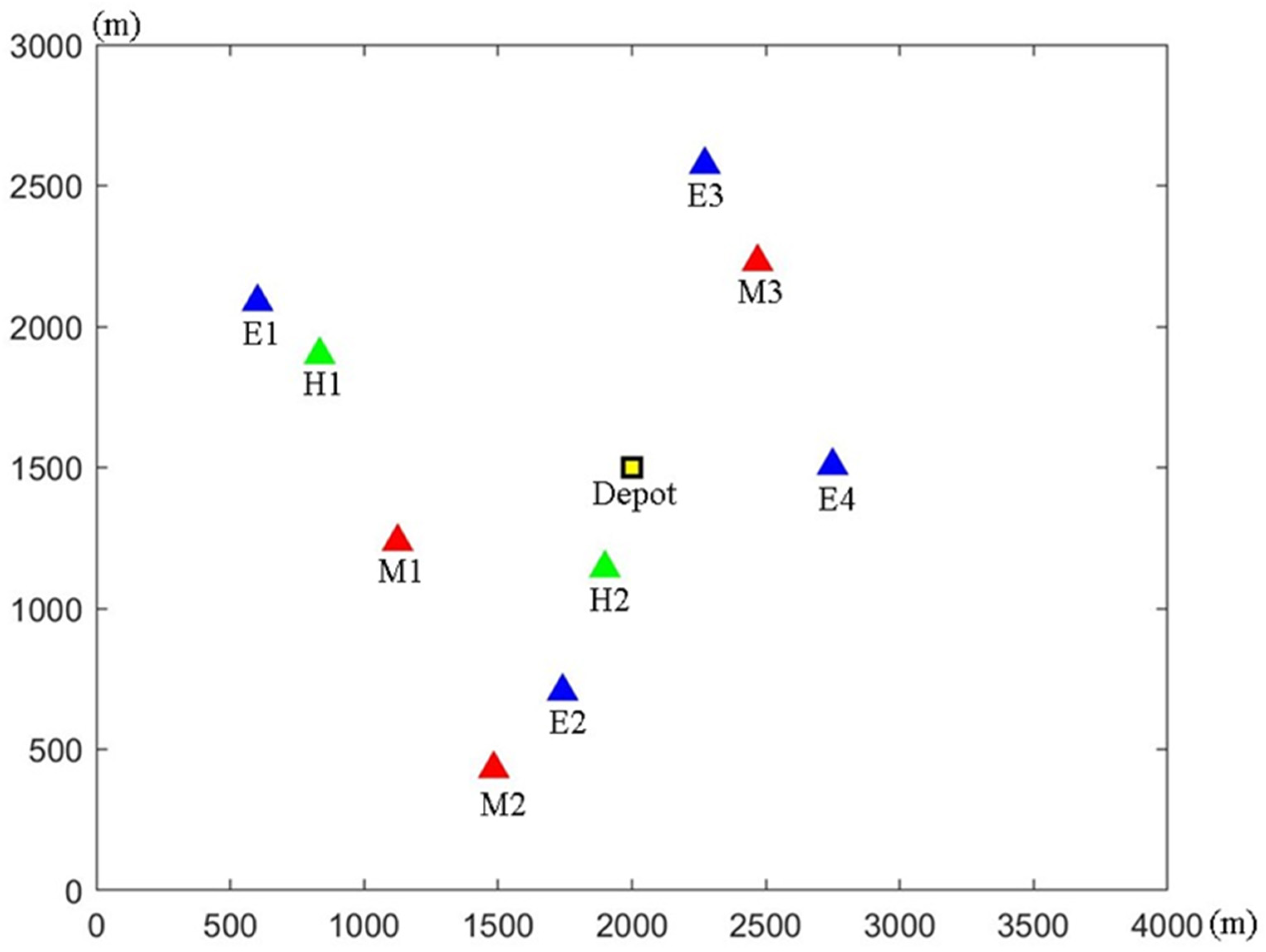
In order to test the algorithm, a hypothetical school bus network consisting of one bus depot, two high schools, three middle schools, and four elementary schools was developed for the simplified school bus operation.

It is assumed that there are 240 students for each level of schools, which means there are 240 students in two high schools (H1 and H2) with 120 students for each high school, three middle schools (M1, M2, and M3) with about 80 students for each middle school, and four elementary schools (E1, E2, E3, and E4) with 60 students for each elementary school; in total, there are 780 students in the network. It is assumed that a total of 12 buses are available, which means that 12 school buses can run every morning and afternoon. Also, it is assumed that each bus has a capacity of 30 seats and that the average speed of each bus is 30 km per hour. The bus operating cost is assumed to be USD 3 per kilometer, and the time value of each student is USD 10 per hour.

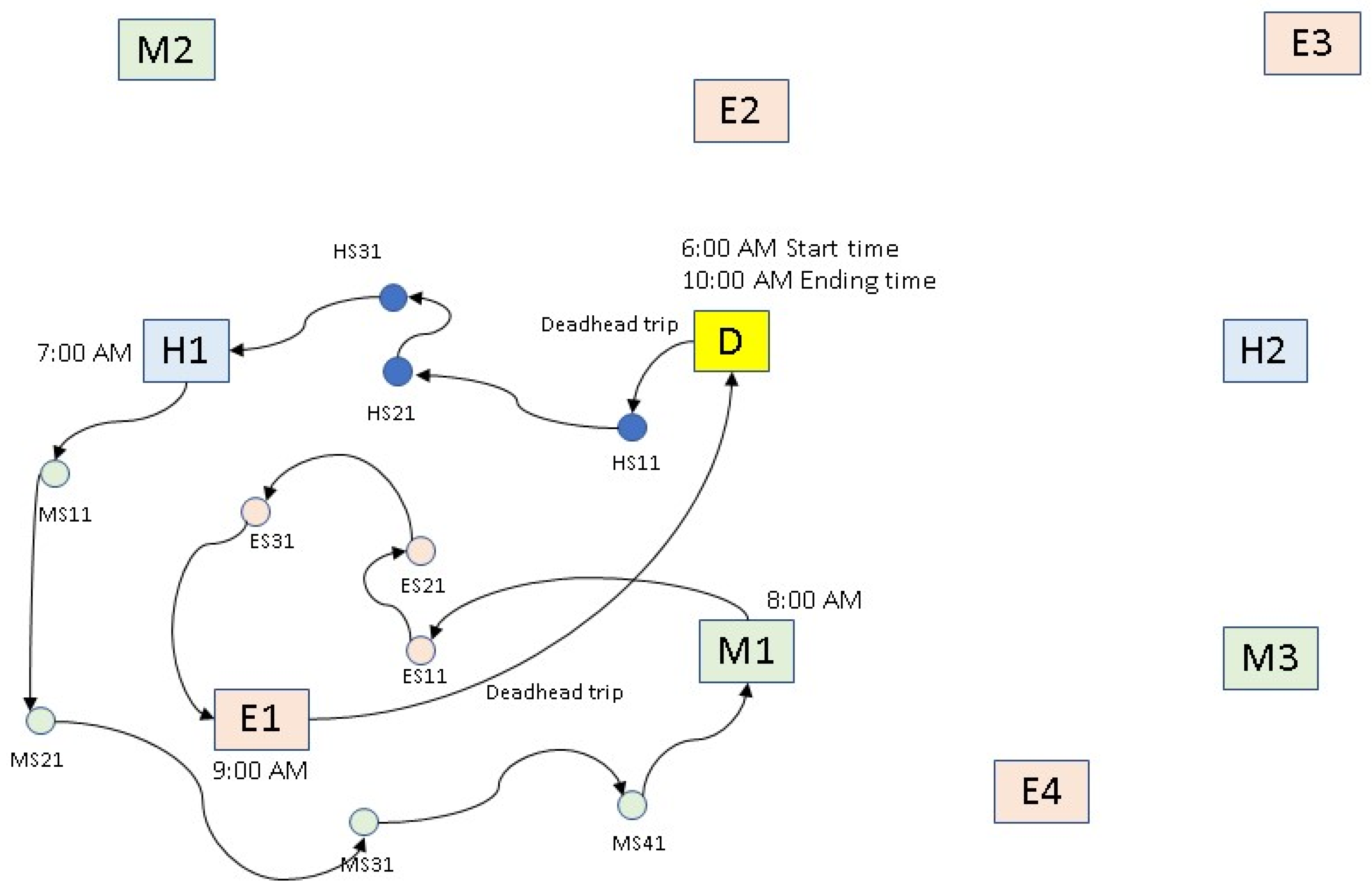
The problem has two separate time periods: morning and afternoon. In the morning, there are three time windows for each time period, and in the first time window (6 a.m. to 7 a.m.), the school buses only serve high school students by picking them up at their location and dropping them at their designated high schools. Then, in the second time window (7 a.m. to 8 a.m.), buses start their trips from high schools and go to middle schools while picking up only middle school students. In the last time window of the morning (8 a.m. to 9 a.m.), the buses start their trips from middle schools to elementary schools to serve elementary students. Finally, after serving all three levels of schools, the buses make deadhead trips to the depot.

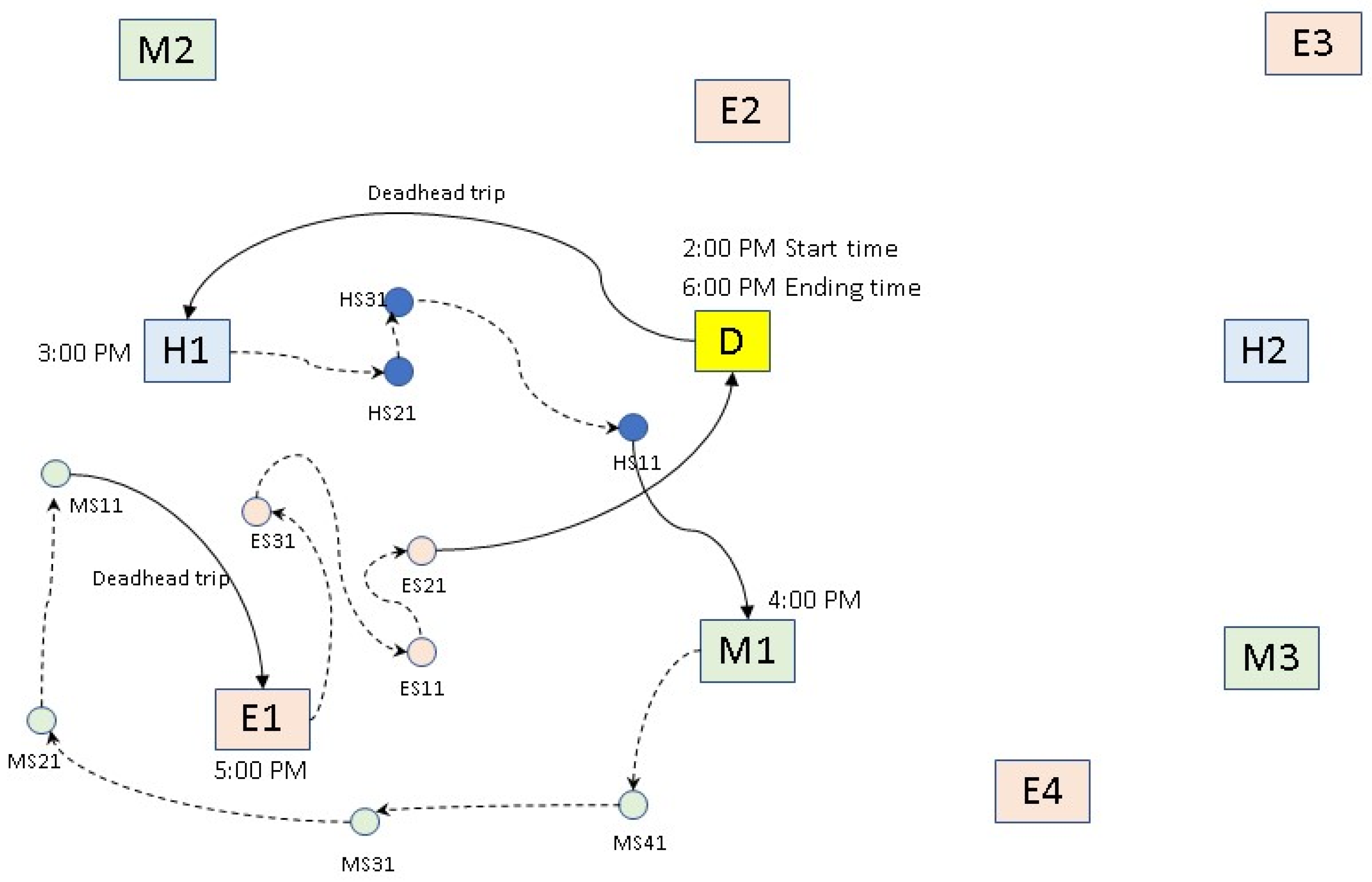
In the afternoon time window, the buses are running in a reverse process from their morning trips. The buses start with deadhead trips from the depot to high schools to pick up high school students at 2 p.m.; then, after delivering students to their stops or homes, the buses go directly to middle schools to pick up and deliver middle school students. After delivering the last student, the buses head to elementary schools to pick up and deliver elementary students. After delivering all elementary students, the buses make deadhead trips to the depot. Figure 1 and Figure 2 show the simplified conceptual operations of school buses during the morning and afternoon time windows. In Figure 2, the sequence of dropping off students may not be the exact opposite of the morning’s picking up sequence, and the routes with different sequences are indicated with dashed lines to show the difference. Also, Figure 3 shows the locations of schools in the example.

6. Results

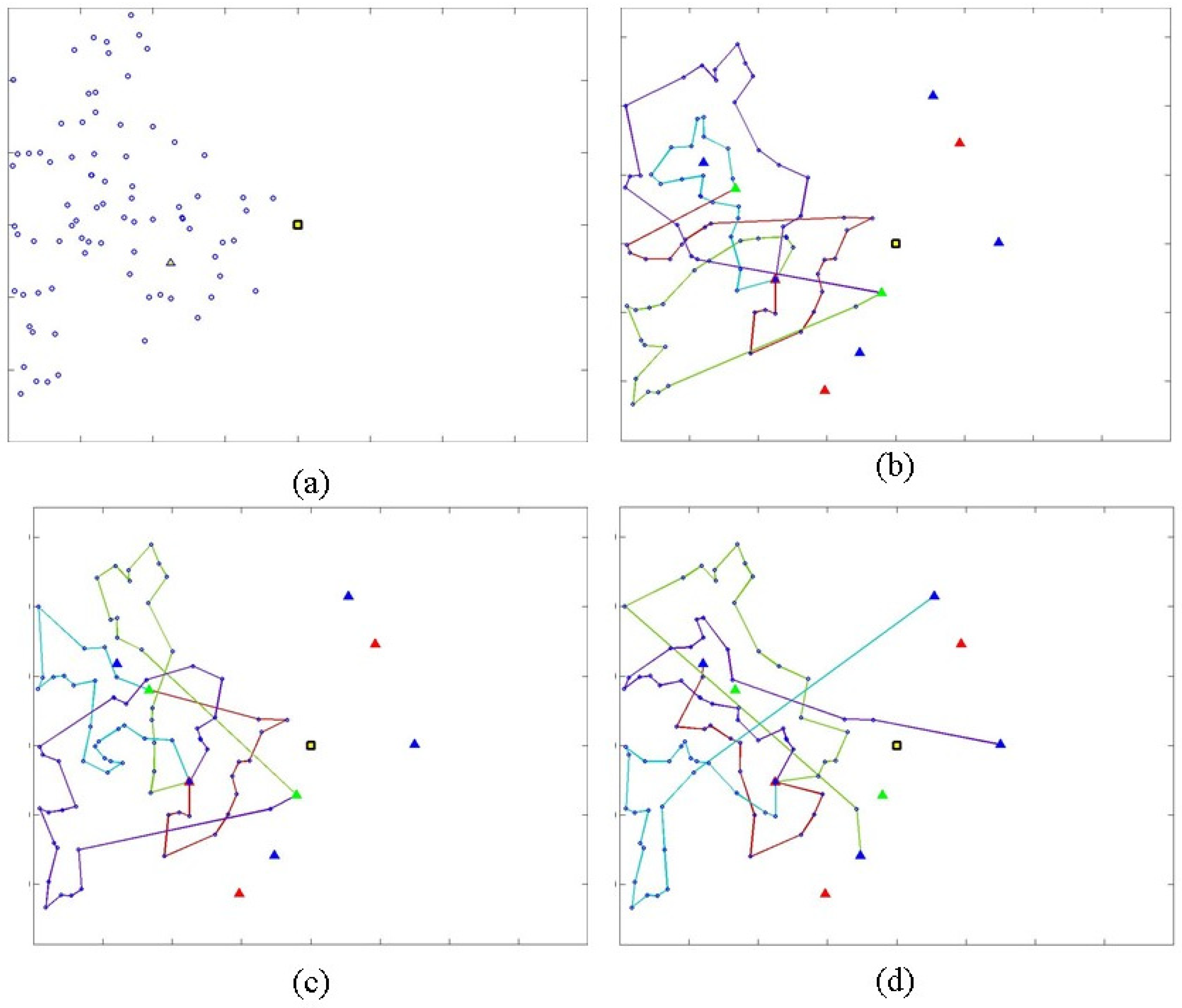
The algorithm successfully generated the school bus routings for both morning (AM) and afternoon (PM) periods. The following Figure 4, as an example, shows the routings in the afternoon period for middle school M1. In these figures, Figure 4a shows the location of students, Figure 4b represents the optimal routing when the routing is the same (identically reversed) for morning and afternoon time windows, Figure 4c represents the optimal routing for the morning time window, and Figure 4d shows the optimal routing for the afternoon time window.

The proposed algorithm provided a solution that optimally minimizes the total costs, including both the travel time of students and school bus operations costs. One of the main complaints of parents whose children use school buses in the U.S. is that their children have to remain on the bus for a long time while their homes are relatively close to the school. To address this issue, the school buses should have different routes for morning and afternoon time windows with different picking up and dropping off sequences that can decrease travel distance and the operating costs of the public school bus service. Although the amount of cost savings depends on the distribution of students and the scale of the problem, theoretically, the total costs of the public school bus operation would be reduced when it comes to choosing different routes for the morning and afternoon time windows.

To compare with the developed integrated single-framework algorithm, identically reversed routings with three separated levels were generated, and their costs were computed as shown in

Table 2. Summarized results of the model.

Routing Status	School	Time Window	Total Student Traveling Time (h)	Total Bus Traveling Distance (km)	Total Students Traveling Cost (USD)	Total Bus Operating Cost (USD)	Total Cost
							(USD)
Different routing for morning and afternoon (integrated framework)	HS	M	12.74	62.61	127.35	187.82	1815.96
	MS	M	12.29	61.6	122.86	184.81
	ES	M	11.18	60.81	111.82	182.44
	HS	A	12.84	59.57	128.4	178.71
	MS	A	11.7	63.61	117.01	190.83
	ES	A	11.96	54.76	119.63	164.27
Identically reversed same routing (integrated framework)	HS	M	14.61	60.22	146.1	180.65	1979.88
	MS	M	13.98	61.5	139.82	184.51
	ES	M	12.42	56.67	124.16	170.02
	HS	A	15.71	60.22	157.09	180.65
	MS	A	17.3	61.5	172.95	184.51
	ES	A	16.94	56.67	169.41	170.02
Different routing for morning and afternoon (separated framework)	HS	M	14.59	64.11	145.90	192.33	2001.64
	MS	M	13.91	63.21	139.10	189.63
	ES	M	12.34	62.48	123.40	187.44
	HS	A	15.78	60.54	157.80	181.62
	MS	A	16.24	63.14	162.40	189.42
	ES	A	17.03	54.1	170.30	162.30
Identically reversed same routing (separated framework)	HS	M	15.15	64.61	151.5	193.83	2072.05
	MS	M	14.56	63.88	145.56	191.65
	ES	M	12.9	63.37	129	190.1
	HS	A	16.34	61.83	163.37	185.5
	MS	A	17.9	65.77	179.01	197.32
	ES	A	17.55	56.57	175.51	169.7

. The computed total cost was USD 2072.05, and it was proved that USD 92.17 could be saved by the identically reversed routings with the integrated single-framework algorithm, which is equivalent to 4.5% savings. Different routings for morning and afternoon with an integrated single-frame algorithm saved USD 256.09 compared to identically reversed routings with a separated framework, which came out to 12.4% savings. This comparison shows that the integrated single-framework algorithm can produce more efficient routings than the separated-framework algorithm.

Moreover, in the present example of this study, the total costs of the integrated routing framework for different morning and afternoon time windows are 8.28% less than the same routings (identically reversed) for morning and afternoon time windows, while the bus operating cost is 1.67% higher when we implement the integrated routing framework for the different routings.

The results of the analysis also show that although high schools, middle schools, and elementary schools serve the same amount of students (240 students) with the same number of total buses (12 buses), the total cost for high schools is more than that of middle schools, and the total cost for middle schools is more than that of elementary schools, as shown in Table 2, because high schools serve the widest area with more dispersed students than do middle schools, and middle schools serve wider areas with more dispersed students than elementary schools do.

Table 3. Comparison of total costs in different scenarios.

Total Cost (USD)	Separated Models	Integrated Framework
The same routing for morning and afternoon (identically reversed)	2072.05	1979.88 (Saves about %4.5)
Different routing for morning and afternoon	2001.64 (Saves about %3.5)	1815.96 (Saves about %12.5)

summarizes comparisons of total costs for different scenarios.

7. Further Discussions

This research developed an optimal integrated school bus routing algorithm that serves three different levels of schools in a single framework. In most U.S. cities, the department of public school education covers all three levels of schools—high schools, middle schools, and elementary schools—and the school buses are delivering all three levels of students with three different time windows. In the morning, the school buses depart from the depot, first collecting and then delivering high school students. The buses depart from the high school to pick up middle school students, and after they are taken to school, the buses gather elementary school students and ferry them to school before returning, empty, to the depot. In the afternoon, the buses depart from the depot and go to high schools to pick up students. They deliver all high school students to their homes, then head to middle schools next, and then elementary schools until all students are delivered. After all deliveries, the buses return to the depot.

This research considers three levels of schools in three separate time windows in a single framework to optimize the entire routing for two different morning and afternoon time windows. This study has provided three main findings. First, the results of the comparison between the developed integrated single-framework algorithm and the identically reversed routing model with three separated levels showed that 4.5% of the total cost could be saved by using the identically reversed routings with the integrated single-framework algorithm. Different routings for morning and afternoon with the integrated single frame algorithm saved 12.4% compared to the identically reversed routings with the separated framework. This comparison showed that the integrated single-framework algorithm can produce more efficient routings than the separated-framework algorithm.

Second, arranging a different order of serving students for two time windows, morning and afternoon, may noticeably change the total costs of the system. In the proposed example of this study, two algorithms were applied; one algorithm generated two routing sets for morning and afternoon time windows, and the other algorithm generated the same (identically reversed) routing sets for morning and afternoon time windows. Obviously, two different routing sets for morning and afternoon time windows minimized total costs compared to the same (identically reversed) routing set since two different routing sets can optimize each time window even though picking up and dropping off locations are identical because buses’ origins and destinations (depot and schools) are different for morning and afternoon time windows. For this particular example, total costs with two different routing sets were 8.28% less compared to the single routing set.

Lastly, the total cost of a school bus transit service can be highly dependent on the geographic distribution of students. The results of our developed algorithm for the proposed example clearly show that although high schools, middle schools, and elementary schools serve the same number of students (240 students) with the same number of total buses (12 buses), total costs for serving high schools were the highest due to the larger area involved to cover more students per school. Likewise, middle school service (per school) costs more than that of elementary schools because of the larger areas covered with more widely dispersed students. Also, the results show a 1% increase in traveling distance results in approximately a 0.99% increase in the total operating cost.

8. Conclusions

This study developed an integrated optimization algorithm for multi-level school bus routing, aiming to enhance efficiency by combining trips for high schools, middle schools, and elementary schools. The research compared cost savings between identical routings for morning and afternoon versus distinct routings for each time window, highlighting the economic and planning benefits of tailored routings. The results of this study clearly showed that the integrated framework appears to be more efficient in terms of the balance between total student travel time, bus travel distance, and operating costs, resulting in a lower total cost. This indicates that, despite any potential complexities of integrating routes for morning and afternoon, the cost savings are significant. The separated framework consistently incurs higher total costs across all school levels (HS, MS, and ES) and time windows (M and A) compared to the integrated framework. This suggests that operating separate routes for the morning and afternoon is less cost-effective than integrating them.

In practical cases and for the implementation of this integrated algorithm, there are some issues that should be considered, such as flexibility in routing. Constraints and/or objectives that allow for dynamic routing in case of unforeseen circumstances like road closures, traffic, or emergencies might be modified. Real-time or historical traffic data to more accurately estimate travel times and avoid traffic congestion should be incorporated. In order to ensure service quality, objectives related to the quality of service, such as minimizing the number of stops each student must endure or ensuring that no student is on the bus for an excessively long duration, can be included. Lastly, equity considerations such as ensuring that the routing algorithm provides equitable service across different neighborhoods and avoiding bias toward certain areas are crucial.

Future studies can consider more aspects of the SBRP, including mixed loads of students, heterogeneous fleets, special-education students (both mixed and not mixed load), students’ walking distance, road network structure, load balancing, and the ability to relocate buses among schools [51].