Flexible Job Shop Scheduling Problem with Fuzzy Times and Due-Windows: Minimizing Weighted Tardiness and Earliness Using Genetic Algorithms

Abstract

The current requirements of many manufacturing companies, such as the fashion, textile, and clothing industries, involve the production of multiple products with different processing routes and products with short life cycles, which prevents obtaining deterministic setup and processing times. Likewise, several industries present restrictions when changing from one reference to another in the production system, incurring variable and sequence-dependent setup times. Therefore, this article aims to solve the flexible job shop scheduling problem (FJSSP) considering due windows, sequence-dependent setup times, and uncertainty in processing and setup times. A genetic algorithm is proposed to solve the FJSSP by integrating fuzzy logic to minimize the weighted penalties for tardiness/earliness. The proposed algorithm is implemented in a real-world case study of a fabric finishing production system, and it is compared with four heuristics adapted to the FJSSP such as earliest due date, critical reason, shortest processing time, and Monte Carlo simulation. Results show that the performance of the proposed algorithm provides efficient and satisfactory solutions concerning the objective function and computing time since it overperforms (more than 30%) the heuristics used as benchmarks.

1. Introduction

The assignment and sequencing of jobs to production resources represent a complex process in most manufacturing companies, even more in flexible job shop systems where the production scheduling problem has been proved to be a nondeterministic polynomial time-hard problem (NP-hard problem) [1,2], and for which optimal solution algorithms cannot provide solutions in reasonable computational times, especially for large and complex production plants. When considering the FJSSP, the concept of a set of machines in series is replaced by a set of work centers, where each work center contains a set of parallel machines that can have different processing times. In the FJSSP, each job follows a production route and can be processed on any machine that makes up a work center [3]. Moreover, the FJSSP requires a detailed discussion of the scheduling of orders importance from the point of due dates [4], implying the consideration of objective functions related to tardiness and earliness [5,6]. However, many FJSSP models proposed in the literature assume conditions far from reality, ignoring the recirculation of jobs in work centers or machines and considering certainty in all the parameters used to perform the production schedule.

In addition, the studies considering parameter uncertainty do not include variables such as setup times dependent on the operation sequence. In most scheduling models, processing time and due dates represent uncertain variables [7,8,9,10,11], and some studies use fuzzy logic theory to create a hybrid genetic algorithm to minimize makespan [12]. Furthermore, production scheduling problems optimizing earliness and tardiness have increased in relevance in recent years due to the growing interest in just-in-time production [13]. In realistic production scheduling problems, jobs finish as close as possible to due dates or within time-windows, due dates (due windows) since the early completion of jobs generates additional production and storage costs and inventory obsolescence; while late completion causes lost sales [5,14]. Therefore, optimal scheduling minimizing earliness and tardiness penalties can improve the economic effects of firms.

On the other hand, the complexity of the FJSSP requires the use of techniques that provide solutions in reasonable computational times to NP-hard problems. These solutions come from artificial intelligence techniques, which have been active in planning and scheduling for four decades [15]. Therefore, many heuristics and metaheuristics such as genetic algorithms, honey bee optimization, artificial bee colony, ant colony optimization, particle swarm optimization, simulated annealing, and hybrid approaches have been proposed to solve the FJSSP [16]. Chaudhry and Khan [17] performed a review of techniques addressing the FJSSP, highlighting ant colony optimization (ACO), artificial bee colony (ABC), artificial immune system (AIS), evolutionary algorithms, greedy randomized adaptive search procedure (GRASP), Integer/Linear programming, neighborhood search (NS), particle swarm optimization (PSO), simulated annealing (SA), tabu search (TS), mathematical programming, deterministic heuristics, hybrid techniques, and miscellaneous techniques. Evolutionary algorithms represent the most used techniques in the literature to solve the FJSSP and cover a wide variety of techniques including Biogeography-based optimization (BBO), Differential evolution (DE), Evolution strategy (ES), Gene expression programming (GEP), Genetic Algorithms (GA), Genetic programming (GP), Harmony Search (HS), Learning classifier system (LCS), Memetic Algorithms (MA), and Estimation of distribution algorithm (EDA). These techniques are effective for minimizing the maximum completion time of the jobs, better known as makespan [18], and they can also assume other objectives, such as reducing delivery times, minimizing tardiness, minimizing earliness, minimizing resource costs, minimizing flow time, and minimizing the number of tardy jobs [15,17].

Within artificial intelligence techniques, genetic algorithms are usually efficient for the optimization of complex systems, represent a good solver for combinatorial problems, provide a wide range of solutions [19], and have been used to solve many problems related to the FJSSP [20], becoming a powerful and successful technique for solving of NP-Hard problems due to the logic of evolutionary principles [21,22]. The genetic algorithm as an evolutionary algorithm has advantages as it is relatively easy to understand and apply and presents fault tolerance [23]. However, although it has been proven that this metaheuristic efficiently solves complex optimization problems, the parameter values must prevent premature convergences and promote the finding of global solutions instead of local solutions [24,25].

Liu, Yang, Xing, and Lu [26] presented a study considering a flexible job shop system, fuzzy parameters, and time windows, introduced a multi-objective programming problem with fuzzy time windows, and solved the problem through a multi-group genetic algorithm. Similarly, Zhang, Collart-Dutilleul, and Mesghouni [27] developed a model that incorporates time windows, capacity, and space constraints and uses mixed integer programming to limit cyclic activities. Shi, Zhang, and Li [26] use a rolling window rescheduling strategy and dynamic scheduling for the FJSSP with fuzzy delivery time, considering a trapezoidal delivery window to minimize energy consumption, maximum makespan, and consumer dissatisfaction, and solving this problem with an immune genetic algorithm.

Other studies have added restrictions to the FJSSP models to adapt to realistic problems and seek to fulfill several objectives considering multi-objective uncertainty environments [25,28]. In this sense, Jamrus et al. [29] propose a model where the processing time can be exact or fuzzy depending on the availability of job data, and the FJSSP is solved using a hybrid algorithm between a genetic algorithm and the particle swarm optimization algorithm. In most of these models, the fuzzy variables receive triangular membership functions due to the ease of their construction. Based on the abovementioned, this article aims to address the FJSSP considering due-window and fuzzy setup times with triangular membership functions to minimize the weighted penalties for tardiness/earliness through a genetic algorithm.

The present study contributes in multiple ways: Firstly, it develops a methodology to calculate the possibility of tardiness and earliness of a job, comparing the due-date time window with the fuzzy set of the completion time and using this result to calculate the penalty of tardiness and earliness in the objective function. Secondly, the study adapts GA and deterministic methods (heuristics and rules) for the specific assumptions of the proposed FJSSP model. Thirdly, it presents a novel solution representation for each chromosome of the GA in two ways, one to calculate the total penalty (objective function) and another for the mutation and crossover operators to minimize the chance of infectable chromosomes, reducing the use of repairing operators and the algorithm computing time. Fourthly, the proposed algorithm solves a real-world case study in the textile sector, demonstrating the algorithm’s applicability to industries with complex production systems.

2. FJSSP Description

Scheduling of job shop production is defined by four main research problems represented by Job Shop Scheduling Problem (JSSP), Flexible Job Shop Scheduling Problem (FJSSP), Dynamic Job Shop Scheduling Problem (DJSSP), and Flow Shop Scheduling Problem (FSSP) [19]. The classical JSSP represents one of the most difficult workshop problems, it assumes that there is no flexibility in the resources (including machines and tools) for each operation of every job. The FJSSP is an extension of the classical job shop scheduling problem allowing an operation to be processed by any machine from a given set [1]. The FJSSP consists of assigning and sequencing n jobs in m work center, each work center can have a different number of machines or resources, and each machine may process more than one type of operation [30]. In the FJSSP, each job is formed by a sequence of consecutive operations, each operation requires one machine, and each operation has to be performed to complete the job. This problem covers two difficulties namely the machine assignment problem (how to assign the operations on the machines) and the operation sequencing problem (how to sequence the operations on the machines) [31]. The general objective of the FJSSP is to improve the organization’s productivity while reducing production consumption by switching over the selectable machine and taking full advantage of the underutilized capacity, adjusting the processing workload on machines [32]. The performance measures, restrictions, and characteristics the model must comply with must be established to define the FJSSP model. The model proposed in this study is based on the following assumptions:

• All machines are available at the beginning of the scheduling horizon and can process only one job simultaneously.
• No job can start an operation until the previously assigned has finished or until a machine is available to perform that operation. Therefore, only one job operation can be executed at a time.
• Processing times are represented by fuzzy numbers and modeled by triangular membership functions.
• Once an operation of a job has started on a machine, it will not be interrupted until it finishes the total number of units of said job.
• Staff is available to perform each operation.
• Machine breakdown or downtime due to maintenance or repairs in the planning horizon are not considered.
• Setup times depend on the job sequence
• Setup times are represented by fuzzy numbers and modeled by triangular membership functions.
• Recirculation is allowed since a machine can perform several processes (not at the same time), so a job can be processed several times on the same machine.
• A time window defines the expected completion time for each job (interval to determine whether a job is completed on time).
• Machines in the same work center may have different processing times.

The mathematical model of the FJSSP is based on the study by Ortiz et al. [33] and Demir and Işleyen [34], where the objective functions minimize the number of late jobs and the Makes-pan, respectively. However, in these studies, the delivery dates are not represented with time intervals but with exact dates, and they do not consider the time of preparation depending on the sequence, for which we present adjustments to the mathematical model. The indices, sets, data, variables, and mathematical model formulation to optimize the FJSSP are as follows:

Indices:
$j$	Job index
$h$	Job index
$i$	Operation index
$k$	Machine index
$l$	Index of the positions in the sequencing
Parameters:
$n$	Total number of jobs
$m$	Total number of machines
$A_{kij}$	Binary parameter to indicate whether operation i of the job j is performed on machine k
$P_{kij}$	Processing time of operation i of the job j on machine k
$S_{kjh}$	Setup time in machine k if job j starts after completing job h
$M$	Very large number
$d_{jA}$	Lower limit of the due window of job j
$d_{jB}$	Upper limit of the due window of the job j
$w_j$	Weighting for job j
$w_T$	Weighting for tardiness
$w_E$	Weighting for earliness
Variables:
$X_{ijkl}$	Binary variable to indicate whether operation i of job j on machine k is sequenced in position l
$V_{ijk}$	Binary variable to assign operation j of job i on machine k
$T{M}_{kl}$	Start time of machine k at position l
$P{S}_{ij}$	Total process time (includes setup time) of operation i of job j
$T{I}_{ij}$	Start time of operation i of job j
$C_j$	Completion time of job j
$T_j$	Tardiness of job j
$E_j$	Earliness of job j

Model:

$$Min Z={\displaystyle \sum }{W}_i\left(T_{i }{W}_T+E_i{W}_E\right)$$

(1)

$$C_j\ge T{I}_{ij}+P{S}_{ij} \forall i,j$$

(2)

$$T_j\ge C_j-d_{jB} \forall j$$

(3)

$$E_j\ge d_{jA}-C_j \forall j$$

(4)

$${{\displaystyle \sum }}_k[(P_{kij}+S_{kjh})\times V_{ijk}]=P{S}_{ij} \forall i,j,h$$

(5)

$$T{I}_{ij}+P{S}_{ij} \le T{I}_{i+1j} \forall j \forall i=1,\dots ,I-1$$

(6)

$$T{M}_{kl}+P{S}_{ij}\times X_{ijkl}\le T{M}_{kl+1} \forall i,j,k \forall l=1,\dots ,L-1$$

(7)

$$T{M}_{kl}\le T{I}_{ij} \left(1-X_{ijkl}\right)\times M \forall i,j,k, l$$

(8)

$$T{M}_{kl}\le T{M}_{kl}\left(1-X_{ijkl}\right)\times M \forall i,j,k, l$$

(9)

$$V_{ijk}\le A_{kij} \forall i,j,k$$

(10)

$${{\displaystyle \sum }}_i{{\displaystyle \sum }}_j{X}_{ijkl}=1 \forall k,l$$

(11)

$${{\displaystyle \sum }}_k{V}_{ijk}=1 \forall i,j$$

(12)

$${{\displaystyle \sum }}_l{X}_{ijkl}=V_{ijk}\forall i,j,k$$

(13)

$$T{I}_{ij}, P{S}_{ij} \ge 0 \forall i,j$$

(14)

$$T{M}_{kl} \ge 0 \forall k,l$$

(15)

$$T_j, E_j \ge 0 \forall j$$

(16)

$$X_{ijkl}\in \left\{0,1\right\} \forall i,j,k, l$$

(17)

$$V_{ijk }\in \left\{0,1\right\} \forall i,j,k$$

(18)

Equation (1) minimizes the total weighted penalty of the jobs given by lateness and promptness, where the earliness of a job is defined as the maximum between zero and the difference between the lower limit of the due window and the completion time of said job $E_j=Max\left( 0 , d_{jA}-C_j \right)$, and the tardiness of a job is defined as the maximum between zero and the difference between the completion time and the upper limit of the due window of said job $T_j=Max\left( 0 , C_j-d_{jB} \right)$. Although the proposed model deals with two performance measures, these are represented in a single objective function (total penalty) that relates them through weights, which allows lateness and promptness to be assessed differently according to the decision-maker preferences. Constraint (2) calculates the completion time of the operations of each job. Constraints (3) and (4) define respectively the tardiness and earliness of each job based on the limits of the due dates. Constraint (5) ensures that the total processing time of each job includes the machine processing time and the setup time. Constraint (6) guarantees the compliance of precedence of operations. Constraint (7) ensures that machines can perform one operation at a time. Constraints (8) and (9) guarantee that any operation starts when the assigned machine is available, and the previous operation is completed. Constraint (10) establishes the relationship between the assigned machines and the operations assigned to those machines. Constraint (11) guarantees that each operation of each job is assigned to a position on a machine. Constraints (12) and (13) ensure that each operation is processed on the assigned machine and position. Constraints (14)–(18) define the variable domains.

3. Genetic Algorithm and Fuzzy Logic for the FJSSP

No efficient algorithm provides an optimal solution in short computing times to a combinatorial optimization problem such as the FJSSP, so it is necessary to use alternatives to complex and analytical methods [10,17]. These models provide optimal solutions in reasonable computational times only for small instances, which is infeasible for realistic problems, so metaheuristics are suggested to find feasible solutions in reasonable computing times [24]. 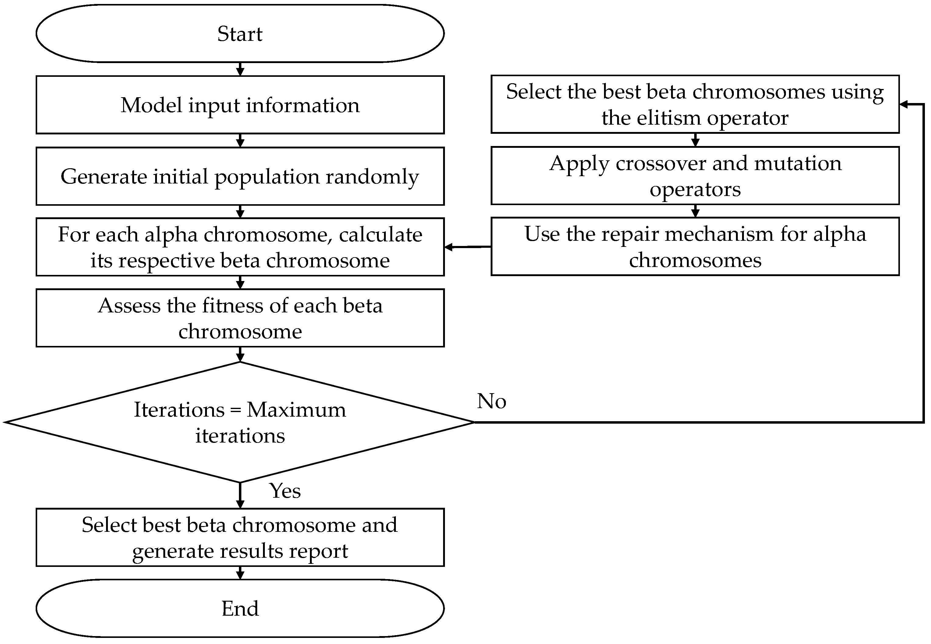Adaptive algorithms for production scheduling in fuzzy environments have delivered good results and have provided excellent solutions; therefore, genetic algorithms have become one of the most used metaheuristics to generate efficient and high-quality job sequences in flexible job shop systems [20,21,29,35]. Thus, this study proposes a genetic algorithm with fuzzy logic that follows the ones described in Figure 1 and detailed below.

Step 1. Enter the weight of each job j ($W_j$), the due window of each job $\left(d_{jA},d_{jB}\right)$, processing routes, available machines, processing times, sequence-dependent setup times, weight of tardiness ($w_T$) and earliness ($w_E$). Enter the genetic algorithm parameters such as Population (PB), Iterations (N), Elitism rate (ET), Crossover rate (PC), Mutation rate (MR).

Step 2. Generate the initial population randomly (number of chromosomes) based on the parameter PB, then calculate the number of operations required to complete all the scheduled jobs. In this step, PB chromosomes are randomly generated and are called alpha chromosomes. Each alpha chromosome represents a solution to the proposed scheduling problem; each gene has an input to assign a job randomly and establish the sequence to perform the operations, and another input to store a random number between 0 and 1 to assign the machine that performs the respective operation. A representation of an alpha chromosome is shown below in Figure 2.

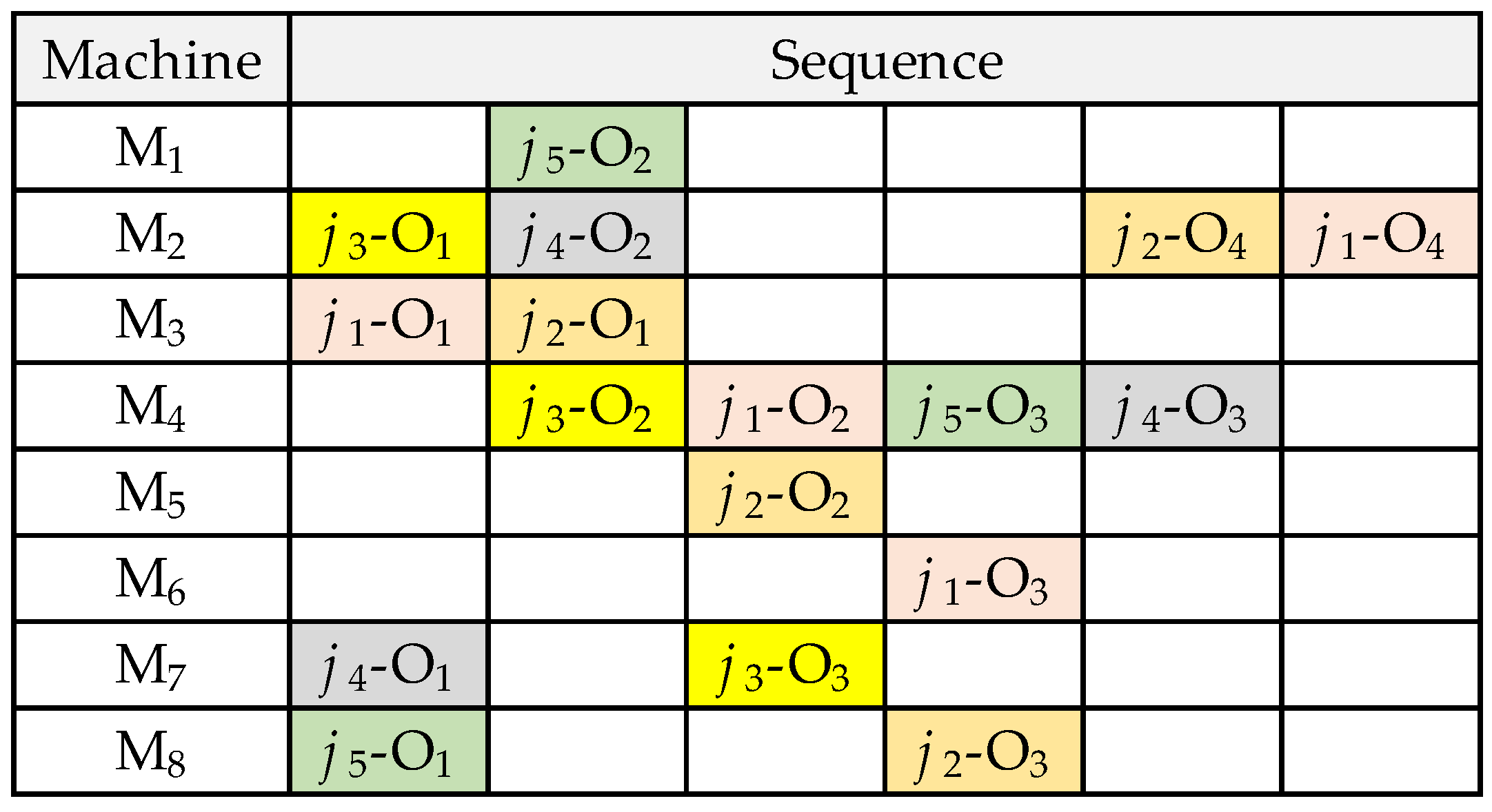
Step 3. Since the alpha chromosome is used to perform the crossover and mutation operators, the beta chromosome facilitates the evaluation of the objective function (fitness value). This chromosome representation enhances offspring feasibility, only requiring the repair of chromosomes by the number of operations per job. The beta chromosomes result from the alpha chromosomes by assigning in input 2 of each gene the machine that performs the operation for the job assigned in input 1. The machine assignment shown in Figure 3 compares the value stored in input 2 of the alpha chromosome with the probability assigned to each machine enabled to perform the operation indicated in input 1. All machines enabled to perform an operation receive the same selection probability. As an example, Figure 4 indicates the sequencing of jobs corresponding to the beta chromosome from Figure 3, where job 3 is shown to be assigned three operations, the first operation is assigned to machine 2 (j₃-O₁), the second operation is assigned to machine 4 (j₃-O₂), and the third operation is assigned to machine 7 (j₃-O₃).

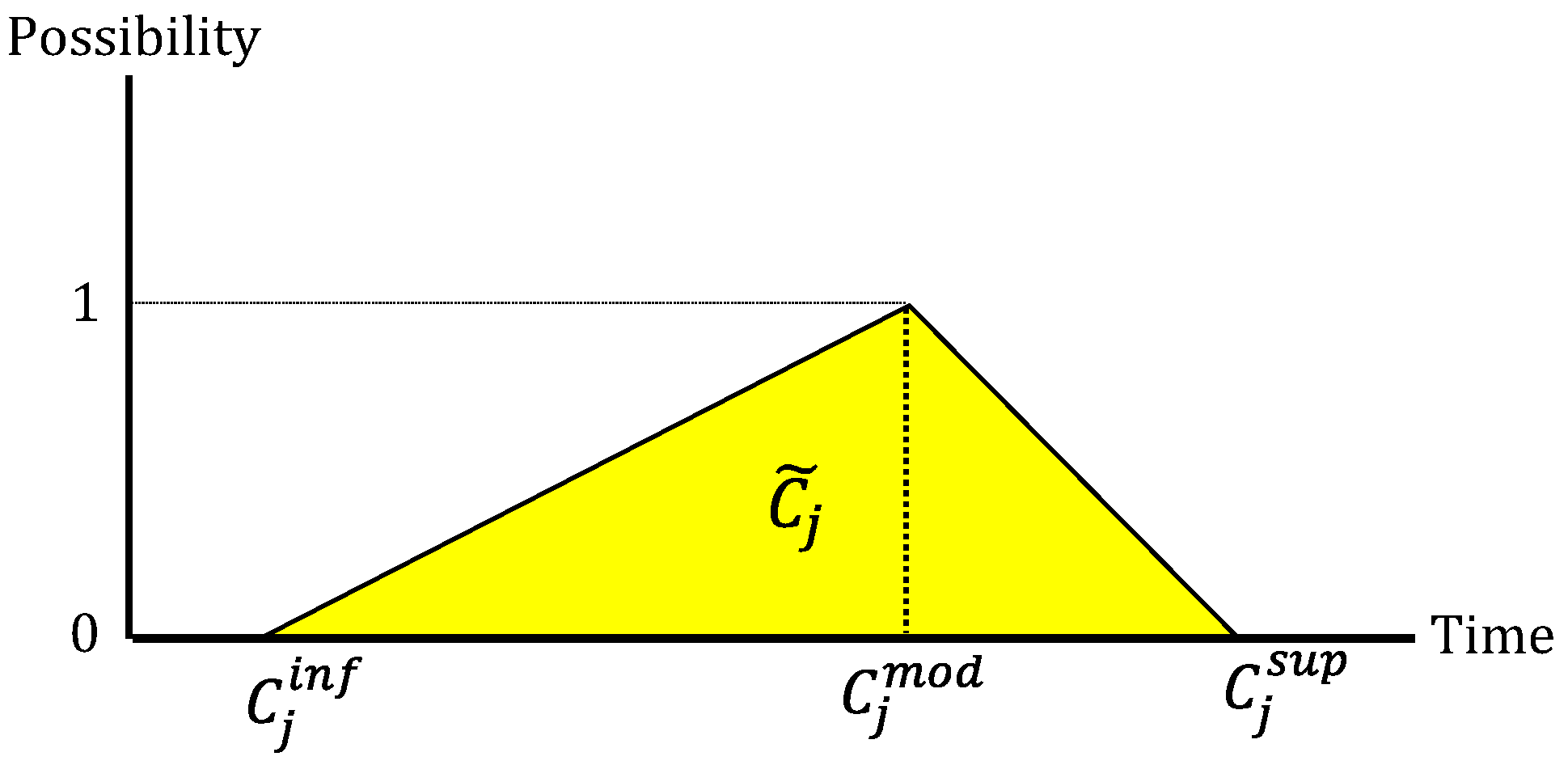
Step 4. The fuzzy completion time $\widetilde{C_j}$ of each job j must be calculated to assess the fitness of each beta chromosome. As shown in Equation (19), the completion time for a selected gene is calculated as the start time of the operation (maximum between the available time of machine i $\widetilde{T{M}_i}$ and the cumulative completion time of job j up to the evaluated gene $\widetilde{C_j }$) plus the setup time in machine i $\widetilde{S_{ilj}}$ and the processing time of operation o of job j in machine i $\widetilde{P_{jio}}$. The available time of machine i will be updated with the completion time of job j that has been processed in this machine ($\widetilde{T{M}_i}=\widetilde{C_j}$). In the proposed methodology, the fuzzy sets used have triangular membership functions such that $\widetilde{C_j}=\left(C_j^{inf},C_j^{mod}{C}_j^{sup}\right)$. The elements that make up the triangular fuzzy number are shown in Figure 5, and these can be calculated following Equations (20)–(22).

$$\widetilde{C_j}=\max (\widetilde{C_j }, \widetilde{T{M}_i})+\widetilde{P_{jio}}+\widetilde{S_{ilj}}$$

(19)

$$C_j^{inf}=\max (C_j^{inf}, T{M}_i^{inf})+P_{jio}^{inf}+A_{ilj}^{inf}$$

(20)

$$C_j^{mod}=\max (C_j^{mod}, T{M}_i^{mod})+P_{jio}^{mod}+A_{ilj}^{mod}$$

(21)

$$C_j^{sup}=\max (C_j^{sup}, T{M}_i^{sup})+P_{jio}^{sup}+A_{ilj}^{sup}$$

(22)

Likewise, it is necessary to calculate the fuzzy tardiness and earliness of each job to obtain the fitness of each chromosome. It requires comparing $\widetilde{C_j}$ with the limits of the due window ($d_{jA}$, $d_{jB}$). The fuzzy tardiness ($\widetilde{T_j}$) is determined by intercepting $\widetilde{C_j}$ with the tardiness interval ($I{T}_j$) that starts at $d_{jB}$ and is not bounded by an upper value $\left( d_{jB} ,+\infty \right)$. The fuzzy earliness of each job j ($\widetilde{E_j}$) is determined by the intercept of $\widetilde{C_j}$ with the earliness interval ($I{E}_j$) that starts at zero and ends at $d_{jA}$ $\left(0 , d_{jA}\right)$. 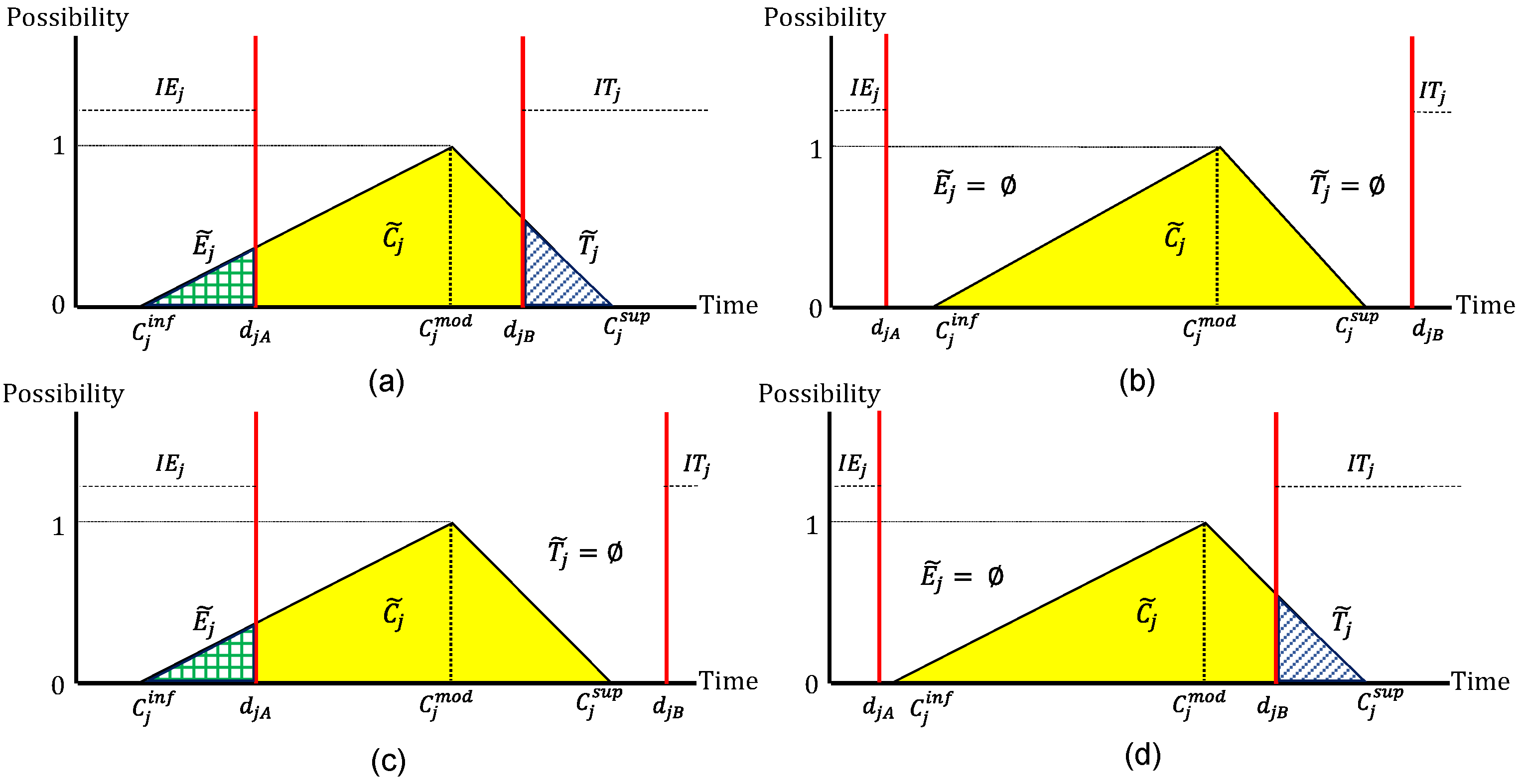Figure 6 illustrates the different cases in which fuzzy delay and fuzzy promptness can be configured. Figure 6a shows the first case where there is the possibility of completing job j early (earliness) or late (tardiness), but there is also the possibility of completing job j within the due window (on time and without penalties). Figure 6b shows the second case where job j cannot be delivered early (earliness) or late (tardiness), assuming a 100% possibility that job j will be completed within the due window despite considering uncertainty. Figure 6c shows the third case where job j cannot be completed late (tardiness), but there is a possibility that job j will be delivered early (earliness); however, when $C_j^{sup}\le d_{jA}$, there is a 100% possibility that job j will be completed early. Figure 6d shows the fourth case where job j cannot be delivered early (earliness), but there is a possibility that job j will be completed late (tardiness); however, when $C_j^{inf}\ge d_{jB}$, there is a 100% possibility that job j will be completed late.

Consequently, in some cases, it cannot be assured with certainty that a job j will be completed with earliness or tardiness, and in some cases, this possibility can be very high or low. Thus, when calculating the total weighted penalty of a job j, the possibility of occurrence of an advance $P_j^E$ or a delay $P_j^T$ will be considered. For this, Equation (23) describes the membership function ${\mu }_{Cj}\left(x\right)$ of the fuzzy completion time $\widetilde{C_j}$, Equations (24)–(26) show the centroid method to defuzzify the fuzzy earliness, and Equations (27)–(29) show the centroid method to defuzzify the fuzzy tardiness and obtain a real number where $E_j^{*}$ and $T_j^{*}$ represent the defuzzification value of earliness and tardiness of job j, $x{\mu }_{Ej}\left(x\right)$ and $x{\mu }_{Tj}\left(x\right)$ represent the membership function of the fuzzy earliness and tardiness.

$${\mu }_{Cj}\left(x\right)=\left\{\begin{array}{cc}0& six\le C_j^{inf}\hfill \\ \frac{x-C_j^{inf}}{c_j^{mod}-C_j^{inf}}& si{C}_j^{inf}<x\le C_j^{mod}\hfill \\ \frac{C_j^{sup}-x}{c_j^{sup}-C_j^{mod}}& si{C}_j^{mod}<x<C_j^{sup}\hfill \\ 0& six\ge C_j^{sup}\hfill \end{array}\right.$$

(23)

$$E_j^{*}=\frac{{{\displaystyle \int }}_{SE}^{.}x{\mu }_{Ej}\left(x\right)dx}{{{\displaystyle \int }}_{SE}^{.}{\mu }_{Ej}\left(x\right)}=\frac{{{\displaystyle \int }}_{SE}^{.}x{\mu }_{Cj}\left(x\right)dx}{{{\displaystyle \int }}_{SE}^{.}{\mu }_{Cj}\left(x\right)}$$

(24)

$$P_j^E=\frac{{{\displaystyle \int }}_{SE}^{.}{\mu }_{Ej}\left(x\right)dx}{{{\displaystyle \int }}_S^{.}{\mu }_{Cj}\left(x\right)}=\frac{{{\displaystyle \int }}_{SE}^{.}{\mu }_{Cj}\left(x\right)dx}{{{\displaystyle \int }}_S^{.}x{\mu }_{Cj}\left(x\right)}$$

(25)

$$E_j=\left(d_{jA}-E_j^{*}\right)\times P_j^E$$

(26)

$$T_j^{*}=\frac{{{\displaystyle \int }}_{ST}^{.}x{\mu }_{Tj}\left(x\right)dx}{{{\displaystyle \int }}_{ST}^{.}{\mu }_{Tj}\left(x\right)}=\frac{{{\displaystyle \int }}_{ST}^{.}x{\mu }_{Cj}\left(x\right)dx}{{{\displaystyle \int }}_{ST}^{.}{\mu }_{Cj}\left(x\right)}$$

(27)

$$P_j^T=\frac{{{\displaystyle \int }}_{ST}^{.}{\mu }_{Tj}\left(x\right)dx}{{{\displaystyle \int }}_S^{.}{\mu }_{Cj}\left(x\right)}=\frac{{{\displaystyle \int }}_{ST}^{.}{\mu }_{Cj}\left(x\right)dx}{{{\displaystyle \int }}_S^{.}x{\mu }_{Cj}\left(x\right)}$$

(28)

$$T_j=\left(T_j^{*}-d_{jB}\right)\times P_j^T$$

(29)

Once the earliness and tardiness of job j ($E_j$ and $T_j$) are obtained, Equation (30) calculates the total weighted penalty of the beta chromosome r or fitness value, considering the weight of earliness ($W_E$), the weight of lateness ($W_T$), and the weighting of job j ($W_j$).

$$Z_r={{\displaystyle \sum }}_1^n{W}_j\left(T_{j }{W}_T+E_j{W}_E\right)$$

(30)

Step 5. After evaluating the beta chromosomes, they are ordered from lowest to highest according to their fitness value (total weighted penalty), and the best chromosomes are selected to form part of the next generation using the elitism rate ($ET\times PB$).

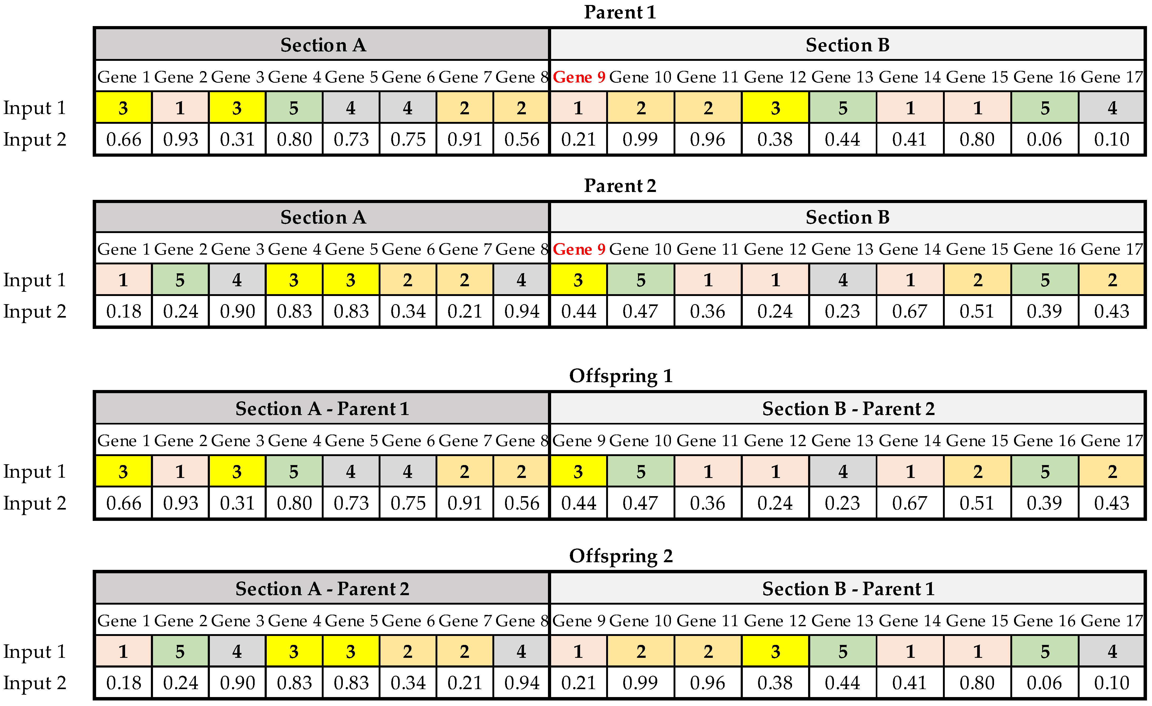
Step 6. The crossover operator completes the next generation by randomly selecting two alpha chromosomes from the current population (parents), then determining with the crossover probability (PC) whether the crossover operation is performed on the parents; or two offspring are generated identically to the parents. In the case of applying the crossover to the selected parents, a single crossing point is randomly chosen to divide each parent into two crossing sections, which are exchanged to form two offspring, as shown in Figure 7.

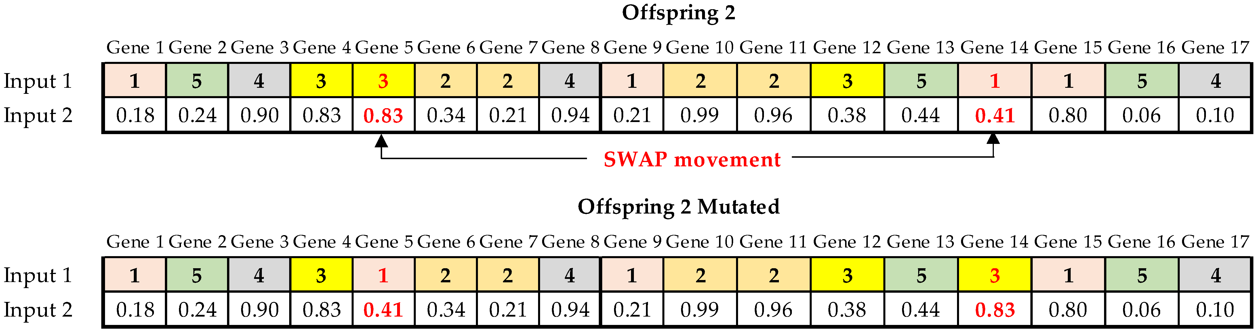
The mutation operator is applied after creating the offspring alphas, generating a random number for each offspring. If this random number is less than the probability of mutation MR, the mutation operation is performed using the swapping mutation method (exchange mutation), where two randomly chosen genes are exchanged through a SWAP movement [36,37] (see Figure 8).

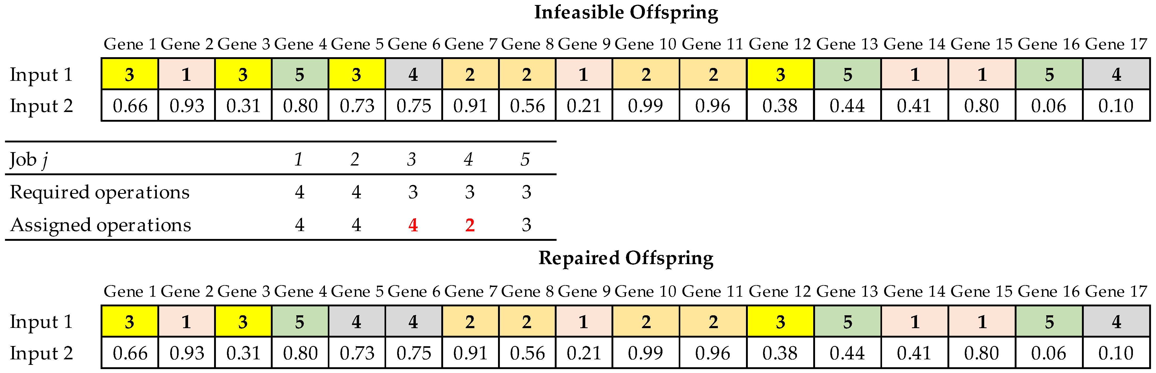
Step 7. After applying the crossover or mutation operator, infeasible offspring may be generated because one or more jobs do not have assigned the number of operations they require, so a job j appears more or fewer times in the offspring than the number of operations it must perform. As shown in Figure 9, the repair mechanism randomly exchanges one of the remaining operations for a missing one.

Step 8. The algorithm returns to Step after creating offspring alpha from the crossover and mutation operations to generate the respective beta chromosome. The fitness value is calculated for each chromosome in the new generation using Step 4.

Step 9. After performing all the iterations N of the algorithm, the best beta chromosome with the lowest total weighted penalty is selected as the best global solution. Then, the corresponding Gantt chart is created to represent the production schedule.

In summary, the basic structure of the proposed GA for the FJSSP is presented below in the Algorithm 1 through its pseudo-code.

Algorithm 1 Genetic Algorithm for the FJSSP

Input Data(); Bestglobal() Generate_initial_population() For p: = 1 to PB Calculate Beta Function();      Beta Fitness Function(); If Mobj(p) < bestfit then bestfit: = Mobj(p); Bestglobal(): = chromosome_beta(p); End if    End for For i: = 1 to Iterations   x: = 0; Sort population(); Elitism operator();   For l: = 1 to int(PB × ET)   x = x + 1; New_population(x): = Sorted_population(l);   End for Crossover Operator(); Mutation Operator(); For l: = 1 to int(PB × (1 − ET))   If Crossover(l) unfeasible then     Correction mechanism();     End if x = x + 1; New_population(x): = Offspring(l);   End for For p: = 1 to PB Calculate Beta Function();     Beta Fitness Function(); If Mobj(p) < bestfit then bestfit: = Mobj(p); Bestglobal(): = chromosome_beta(p); End if    End for End for Output Data();

4. Experiments

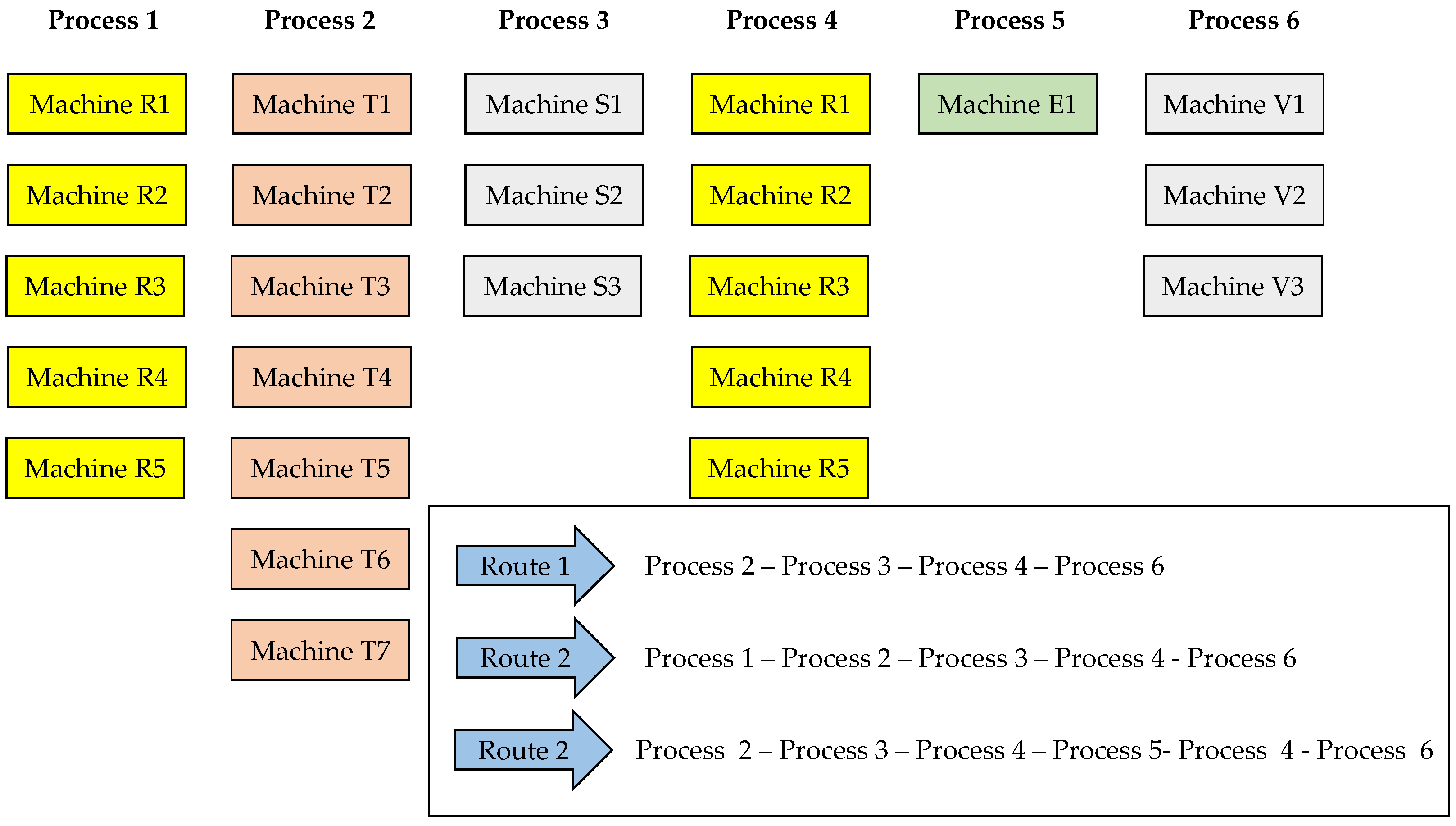
A scheduling problem was approached in a company dedicated to providing fabric finishing services to test the effectiveness of the proposed genetic algorithm in realistic environments. The production system has six processes or stages, 19 machines, some of which can perform more than one process (recirculation condition), and different processing routes for the products to be processed. The setup times are dependent on the schedule sequence due to color changes in the fabrics, and two scenarios of 20 and 30 jobs make up the production schedule. Figure 10 shows the production system highlighting the six processes, the machines enabled by each process, and the routes established within the production plant.

In order to execute and evaluate the proposed genetic algorithm, this study considers a 2k design of experiments for parameter tuning, taking as experimental factors the population (30, 50), number of iterations (1000, 2000), mutation rate (0.03, 0.1), and crossover rate (0.8, 0.9) based on the values proposed by Coello [38], Teekeng and Thammano [39], and Ruiz [40], and considering the conditions of the productive system addressed. The results of the parameter tuning are shown in

Table 1. Genetic algorithm parameter values.

Parameter	Value
Elitism rate	0.1
Mutation rate	0.1
Crossover rate	0.9
Population	50
Iterations	2000

. The number of jobs to be tested is equivalent to 20 and 30 production orders (jobs) because it represents an appropriate size of operations for the fabric finishing plant, in which processing times are high for each production order. The tardiness and earliness weighting parameters of the objective function for the production system are $w_T=1$ and $w_E=0.4$.

The genetic algorithm was compared with four heuristics to evaluate the effectiveness and performance of solving the FJSSP. The selected heuristics were EDD (Earliest Due Date), CR (Critical Reason), SPT (Shortest Processing Time), and Monte Carlo simulation. These heuristics were used in the production scheduling problems addressed by Salazar and Figueroa [41], Wang and Li [35], and González [42]. Likewise, three of these heuristics represent conventional priority rules (EDD, SPT, CR) that have been used by Ojstersek, Tang, and Buchmeister [4]. The adaptation of each heuristic to the flexible job shop system with fuzzy processing times and due windows is explained below.

4.1. Heuristic EDD

The heuristic EDD sequences the jobs according to the due date. This heuristic favors the highest priority jobs; however, it does not take advantage of reducing the setup times when successively processing jobs from the same family [43].

The first step of the heuristic calculates the average delivery time of each job j $d_{jM}$ by averaging the lower limit of the time window $d_{jA}$ and the upper limit of the time window $d_{jB}$, then the jobs are ranked from lowest to highest according to this value. In Step 2, the jobs are sequenced according to the ranking obtained in Step 1, forming a chromosome as in the genetic algorithm, with the difference that all the operations of each job j are located according to their average delivery time. Figure 11 shows an example of a solution (chromosome) sequencing five jobs (1, 2, 3, 4, and 5), which have 4, 4, 3, 3, and 3 operations, respectively. The order of the jobs according to their average delivery time is 3, 5, 2, 1, and 4.

In Step 3, the machine with the shortest time to complete the operation is assigned, allowing it to complete the operation in the shortest time. For this, it is necessary to defuzzify the processing times of the operation in each machine and the sequence-dependent setup times (for triangular functions, average the lower value, the mode value, and the upper value). Equation (31) shows that this result is added to the maximum between the available start time of the evaluated machine and the completion time of the previous operation of the processed job. After assigning the machines, the EDD heuristic solution shows the sequence of jobs, operations, and assigned machines (see Figure 11). In Step 4, the fitness of the chromosome constructed with the EDD heuristic is evaluated using the same procedure proposed to assess a beta chromosome generated by the proposed genetic algorithm.

$$C_j^{desf}=\max (C_j^{defu}, T{M}_i^{defu})+P_{jio}^{defu}+A_{ilj}^{defu}$$

(31)

4.2. Heuristic CR

The CR heuristic builds a sequence of jobs, ordering them from lowest to highest according to the value of the ratio between the remaining time to their delivery commitment and the remaining process time [41]. In the proposed problem, the remaining time to the delivery commitment of each job j is equal to the average delivery time of each job j, and the remaining processing time of each job j is equal to the sum of the average times of the operations that must be performed on different machines. For the problem addressed in this study, the CR heuristic is based on the following steps.

Calculate the average delivery time, total processing time, and sort jobs. For each job j, the average delivery time $d_{jM}$ must be calculated by averaging the lower limit of the time window $d_{jA}$ and the upper limit of the time window $d_{jB}$. Then the expected total processing time $P_j^{total}$ shown in Equation (32) must be calculated by adding the average processing times of each operation of job j. To calculate the average processing times in operation o of job j ($P_{jo}^{prom})$ shown in Equation (33) it is necessary to calculate the defuzzified processing time for job j on machine k ($P_{jok}^{defu}$), where $X_{jok}$ represents a binary variable that takes the value of 1 when machine k is enabled to perform operation o of job j. The critical ratio is calculated for each job $(C{R}_j)$ using Equation (34) and the jobs are ranked from lowest to highest according to this value. After sorting the jobs j according to the critical ratio, steps 2, 3, and 4 are applied in the same way as the EDD heuristic, thus obtaining the sequence and assignment for the FJSSP.

$$P_j^{total}={{\displaystyle \sum }}_{o=1}^O{P}_{jo}^{prom}$$

(32)

$$P_{jo}^{prom}=\frac{{{\displaystyle \sum }}_{k=1}^K{X}_{jok}{P}_{jok}^{defu}}{{{\displaystyle \sum }}_{k=1}^K{X}_{jok}}$$

(33)

$$C{R}_j=\frac{d_{jM}}{P_j^{total}}$$

(34)

4.3. Heuristic SPT

This heuristic indicates that the priority of the jobs to be processed must depend on the shortest processing time. In Step 1, calculate the total processing time for each job j $P_j^{total}$ using Equation (32), and then calculate the average processing time in operation o of job j ($P_{jo}^{prom})$ shown in Equation (33). Jobs are ranked from lowest to highest based on $P_j^{total}$. Then, Steps 2, 3, and 4 of the EDD heuristic are applied, thus obtaining the sequence and assignment for the FJSSP.

4.4. Monte Carlo Simulation

The Monte Carlo simulation randomly generates N solutions to select the schedule with the best result in the objective function. In Step 1, N chromosomes are created, and the jobs are randomly assigned to establish the sequence of operations. Figure 12 shows an example of a solution (chromosome) sequencing five jobs (1, 2, 3, 4, and 5), which have 4, 4, 3, 3, and 3 operations, respectively. Then, Step 3 and Step 4 of the EDD heuristic are applied to each chromosome, obtaining the fitness value of each solution. Finally, the solution that provides the best fitness value is selected. A total of 2000 iterations (random solutions) will be used to compare this heuristic with the proposed genetic algorithm.

The genetic algorithm and heuristics used as benchmarks were coded in Visual Studio 2013 developed by Microsoft Corporation (Redmond, Washington, USA), and the experimental instances were tested on a PC (CPU Intel Xeon (4-Core) E3-1220v5-3.0GHz, 16 GB RAM).

5. Results

When executing the different selected heuristics and comparing them with the proposed genetic algorithm, the following results were obtained in the scenarios considering 20 and 30 jobs.

Table 2. Results for the GA compared to the benchmarks.

Algorithm	Total Weighted Penalty		% Savings
	j = 20	j = 30	j = 20	j = 30
Genetic algorithm	442.94	980.95	-	-
Heuristic EDD	672.33	1420.79	34.12%	30.96%
Heuristic SPT	788.25	1596.87	43.81%	38.57%
Heuristic CR	626.18	1423.51	29.26%	31.09%
Monte Carlo Simulation	666.94	1510.56	33.59%	35.06%

shows the efficiency of the proposed algorithm over the selected heuristics, highlighting that the proposed genetic algorithm exceeds the benchmark solution by an average of 34.56%, obtaining savings of up to 43.81% compared to the SPT heuristic when considering 20 jobs and providing savings of up to 38.57% compared to a heuristic widely used in production systems such as the EDD heuristic when considering 30 jobs. Therefore, the proposed genetic algorithm provides efficient solutions to realistic problems in flexible job shop systems with sequence-dependent setup times.

Likewise,

Table 3. Completion time for the best solution considering 20 jobs.

Job j	Due Window		Completion Time
	${\mathit{d}}_{\mathit{j}\mathit{A}}$	${\mathit{d}}_{\mathit{j}\mathit{B}}$	${\mathit{C}}_{\mathit{j}}$	${\mathit{C}}_{\mathit{j}}^{\mathit{i}\mathit{n}\mathit{f}}$	${\mathit{C}}_{\mathit{j}}^{\mathit{m}\mathit{o}\mathit{d}}$	${\mathit{C}}_{\mathit{j}}^{\mathit{s}\mathit{u}\mathit{p}}$
1	64	72	55.6	51.3	55.4	60.1
2	78	102	97.2	90.9	96.7	104.1
3	58	72	61	56.4	60.9	65.6
4	50	62	32.6	30.3	32.4	35.1
5	98	110	99.1	91.8	98.5	107
6	80	92	63	58.2	62.9	67.8
7	106	116	103.6	97.1	103.1	110.8
8	200	216	165.5	152.6	164.7	179.1
9	128	136	119.1	111	118.4	127.9
10	224	232	117.7	109.8	117	126.3
11	193	215	120.7	112.5	120	129.6
12	267	287	122.6	114.2	121.9	131.7
13	272	288	163.9	151.2	163.1	177.3
14	296	312	129.4	119.9	128.6	139.6
15	192	208	146.5	135.8	145.8	157.9
16	360	376	162.8	150.3	162.1	176.1
17	288	304	140.9	130.9	140.3	151.6
18	260	272	156.4	144.4	155.7	169.2
19	318	328	159.6	147.3	158.9	172.7
20	198	209	99.6	93.1	99.1	106.6

and

Table 4. Completion time for the best solution considering 30 jobs.

Job j	Due Window		Completion Time
	${\mathit{d}}_{\mathit{j}\mathit{A}}$	${\mathit{d}}_{\mathit{j}\mathit{B}}$	${\mathit{C}}_{\mathit{j}}$	${\mathit{C}}_{\mathit{j}}^{\mathit{i}\mathit{n}\mathit{f}}$	${\mathit{C}}_{\mathit{j}}^{\mathit{m}\mathit{o}\mathit{d}}$	${\mathit{C}}_{\mathit{j}}^{\mathit{s}\mathit{u}\mathit{p}}$
1	64	72	34.5	32.1	34.4	36.9
2	78	102	100.7	93.1	100.4	108.5
3	58	72	99.4	91.9	99	107.1
4	50	62	107.5	99.1	107.1	116.2
5	98	110	114.9	105.5	114.5	124.5
6	80	92	29.2	27.4	29	31.1
7	106	116	135.7	125.6	135.3	146.2
8	200	216	138	127.8	137.6	148.6
9	128	136	121.8	112.2	121.4	131.7
10	224	232	102.1	94.5	101.7	110.1
11	193	215	119.8	109.9	119.3	130
12	267	287	63.6	60	63.2	67.7
13	272	288	161	148.1	160.6	174.4
14	296	312	177	163.1	176.5	191.4
15	192	208	179.8	166.3	179.3	193.9
16	360	376	149.9	138.3	149.5	162.1
17	288	304	161.7	149.4	161.3	174.3
18	260	272	180.5	166.3	179.9	195.2
19	318	328	171.3	157.8	170.8	185.2
20	198	209	173.6	160	173.1	187.7
21	312	317	160	147.2	159.5	173.3
22	174	182	104.6	96.8	104.2	112.9
23	222	230	168	155.5	167.6	180.9
24	342	350	181.5	167.8	181	195.7
25	400	404	163.5	150.4	163	177
26	406	420	178	164.6	177.5	192
27	392	400	140.6	130.1	140.1	151.4
28	440	448	182.1	167.9	181.5	197
29	296	304	183	169.1	182.5	197.4
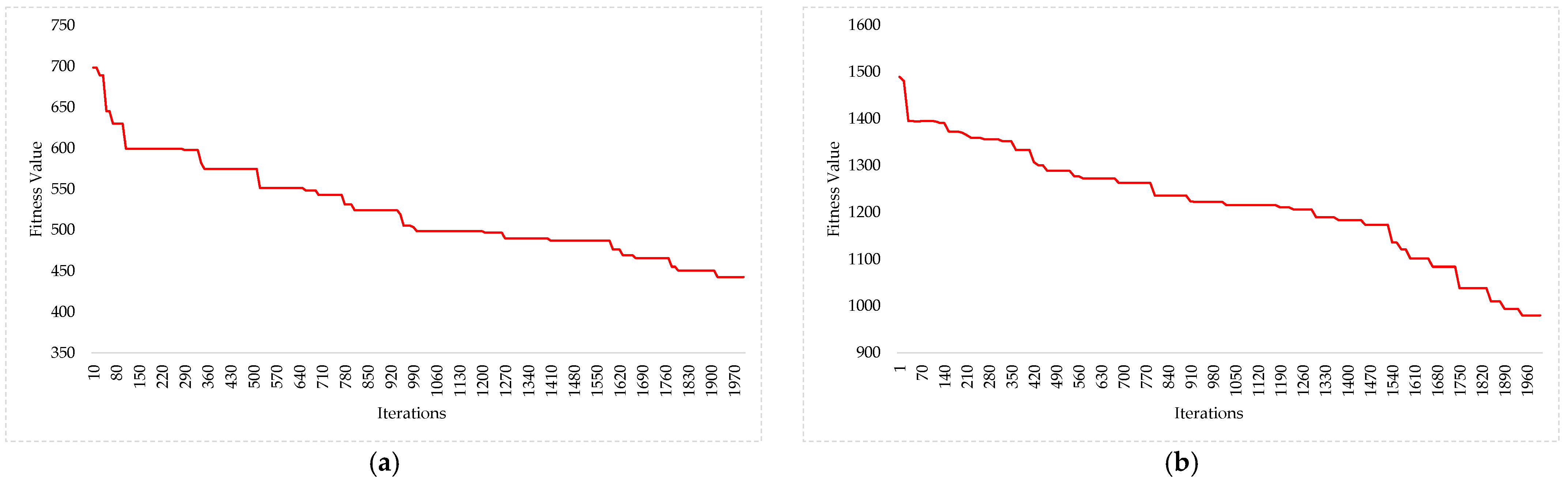
30	416	424	177.7	163.8	177.2	192.2

show the completion time of the jobs that make up the best solution obtained with the genetic algorithms when considering 20 and 30 jobs, respectively, which generated a weighted penalty value equal to 442.93 and 980.95.

Figure 13a,b respectively shows the evolution of the fitness value with the genetic algorithm throughout the generations (iterations) planned for the 20 and 30 jobs within the production system of the fabric finishing plant. Therefore, the algorithm is convergent because as the number of iterations (generations) increases, the solution obtained notably improves its total weighted penalty value. For the case of 20 jobs, after 1700 iterations, the improvements are reduced, while in the case of 30 jobs, upon reaching 2000 iterations, significant advances continue appearing in the objective function.

In addition to the analysis of the objective function of this study,

Table 5. Number of tardy jobs for the GA compared to the benchmarks.

Algorithm	Number of Tardy Jobs Based on Possibilities		% Savings
	j = 20	j = 30	j = 20	j = 30
Genetic algorithm	1	5	-	-
Heuristic EDD	5	15	80.0%	66.7%
Heuristic SPT	6	17	83.3%	70.6%
Heuristic CR	4	12	75.0%	58.3%
Monte Carlo Simulation	5	14	80.0%	64.3%

and

Table 6. Average possibility of tardy jobs for the GA compared to the benchmarks.

Algorithm	Average Possibility of Tardy Jobs		% Savings
	j = 20	j = 30	j = 20	j = 30
Genetic algorithm	0.50%	10.72%	-	-
Heuristic EDD	12.05%	47.06%	95.9%	77.2%
Heuristic SPT	13.96%	52.16%	96.4%	79.4%
Heuristic CR	9.55%	39.05%	94.8%	72.5%
Monte Carlo Simulation	12.79%	44.14%	96.1%	75.7%

present other performance indicators such as the number of tardy jobs (based on possibilities), and the average possibility of tardy jobs, where it is considered that a job j has tardiness possibility when $C_j^{sup}>d_{jB}$. Based on the results, the solution obtained with the GA provides only one job that can be late with a 0.50% chance when considering 20 jobs, while five jobs can be late with a 10.72% chance when considering 30 jobs. Likewise, the GA provides average savings of 79.6% in the number of late jobs compared to the benchmarks considering 20 jobs and maximum savings of 83.3% compared to the SPT heuristic. Similarly, GA provides average savings of 65.0% in the number of tardy jobs compared to the benchmarks considering 30 jobs and maximum savings of 70.6% compared to the SPT heuristic. Regarding the average possibility of tardy jobs, GA provides average savings of 95.8% compared to the benchmarks considering 20 jobs and average savings of 76.2% considering 30 jobs. Thus, it is confirmed that the proposed GA, in addition to providing satisfactory solutions in the weighted tardiness and earliness penalty, also provides satisfactory solutions regarding the possibility and number of tardy jobs.

Regarding computing time, the genetic algorithm requires an average of 10.5 min to find the best solution when considering 20 jobs and 2000 iterations, while it requires 17.6 min to find the best solution when considering 30 jobs and 2000 iterations. When comparing the computing time for 20 jobs against 30 jobs (50% increase in the number of jobs), the computing time increases on average by 68.3%, showing the combinatorial complexity and NP-hard nature of the FJSSP with sequence-dependent setup times. In this sense, it is relevant that decision-makers consider the trade-off between the solution quality and the computing time of the genetic algorithm to obtain satisfactory solutions in reasonable times for production systems.

6. Conclusions

This study addresses for the first time FJSSP in fuzzy environments considering parameters and constraints of real production systems such as sequence-dependent setup times, due windows, recirculation, and consideration of earliness and tardiness in objective functions. Due to the complexity of the FJSSP, it is necessary to use artificial intelligence techniques such as genetic algorithms, which provide satisfactory solutions in reasonable computation times. One of the main contributions of this article is the proposal of a genetic algorithm and four heuristics since they represent one of the first approaches to tackle the FJSSP considering the realistic conditions presented in this study and applied to a fabric finishing production system.

When comparing the results of the proposed genetic algorithm with different heuristics, it was possible to verify that, in all cases, the proposed methodology exceeded the performance of the heuristics by more than 30%, which shows the effectiveness of the proposed algorithm. Additionally, the GA provides satisfactory solutions regarding the possibility and number of tardy jobs. Moreover, the computing time of the genetic algorithm is viable for operating environments; therefore, it can be used daily in flexible job shop systems once the production orders are available. These results showed that the proposed genetic algorithm provides the best solutions for the FJSSP, outperforming heuristics widely used in production systems. Consequently, this study reduces the penalties related to earliness and tardiness and flexible job shop systems, increasing customer service and storage costs, inventory obsolescence, and lost sales.

Despite the contributions of the study, it still has some flaws. In the future, datasets such as BRdata [44], Kacem data [45], BCdata [46], and HUdata [47] can be used to test the efficiency and effectiveness of the proposed GA, and compare its performance with other metaheuristics such as ACO, ABC, AIS, NS, SA, TS, PSO, hybrid metaheuristics, and other evolutionary algorithms. Likewise, future studies could include orthogonal experiments for parameter tuning for both the genetic algorithm and the metaheuristics used as benchmarks. Future works could consider changes in work speed, limitations in transportation and storage within the production system, machine downtime, and stockout probabilities. Moreover, the proposed algorithm could be complemented with a local search algorithm to improve the fitness of the chromosomes and reduce the number of iterations necessary to find a satisfactory solution.