Article

Blocking Cyclic Job-Shop Scheduling Problems

by
Atabak Elmi
1,
Dhananjay R. Thiruvady
1,* and
Andreas T. Ernst
2
1
School of Information Technology, Faculty of Science, Engineering and Built Environment, Deakin University, Geelong, VIC 3125, Australia
2
School of Mathematics, Faculty of Science, Monash University, Melbourne, VIC 3800, Australia
*
Author to whom correspondence should be addressed.
Algorithms 2022, 15(10), 375; https://doi.org/10.3390/a15100375
Submission received: 1 September 2022 / Revised: 7 October 2022 / Accepted: 10 October 2022 / Published: 14 October 2022

Abstract

:
Cyclic scheduling is of vital importance in a repetitive discrete manufacturing environment. We investigate scheduling in the context of general cyclic job shops with blocking where there are no intermediate buffers between the machines. We also consider sequence-dependent setups (anticipatory and nonanticipatory), which commonly appear in different manufacturing environments. The choice of blocking condition, that is whether the sequence-dependent setups are anticipatory or not, significantly impacts the optimal schedules. We provide a novel mixed-integer programming (MIP) model for the above problem, namely blocking cyclic job-shop scheduling. Furthermore, we study the impact of sequence-dependent setups in this research. The problem is analysed in detail with respect to anticipatory and nonanticipatory setups and the efficiency of the proposed model is investigated via a computational study that is conducted on a set of randomly generated problem instances. The proposed MIP models are capable of solving small-to-medium-sized problems. Moreover, the analysis presented demonstrates that anticipatory setups directly affect blocking conditions, since intermediate buffers between the machines are not present. Hence, in systems with anticipatory setups, cycle times increase to a greater extent compared to systems with nonanticipatory setups.

1. Introduction

This study is concerned with a manufacturing system, namely cyclic job shop with blocking conditions. The cyclic job-shop scheduling problem is an extension of the well-known job-shop scheduling problem (JSSP) [1,2]. The original JSSP involves scheduling jobs, each of which consist of a number of operations, and the objective is to minimise the length of the schedule, or the makespan. Moreover, manufacturing systems often require schedules that are cyclic in nature and leading to additional complexities [3,4]. Cyclic or periodic scheduling produce schedules that are executed repeatedly in exactly the same manner on one or more machines [5]. The objective functions mainly used in cyclic scheduling are minimising cycle time, work-in-process, and mixes of them. The cycle time is the time period between two successive occurrences of the same operations, and the work-in-process is the number of jobs processed at the same time. The aim of cyclic scheduling in this research is to find a schedule with the minimum cycle time (common in manufacturing systems) [6]. Within the system, a set of jobs, known as the minimal part set (MPS) (For example, if the requirements are 1000 parts of type A, 3000 parts of type B and 2000 parts of type C, the MPS can be chosen as (A, B, B, B, C, C) and we repeat the production of the same MPS 1000 times.) is executed cyclically, in order to meet production requirements [7,8]. Referring to parts as jobs, for each MPS, the jobs go through the machines in exactly the same pattern, and each machine thereby processes the operations in an identical way in each cycle. An alternative view is that a single MPS is sent into a production line where exactly one MPS is completed and unloaded from it. The primary performance measure is the cycle time, or equivalently its reciprocal, the throughput rate, which measures how often the MPSs are produced in a fixed time interval. The JSSP itself is known to be among the most complex combinatorial optimisation problems [9], and the cyclic variant considered in this study incorporates further complexity.
Moreover, in several manufacturing systems, there exist production processes where no intermediate buffers exist between machines due to technical requirements or process characteristics. In the context of the JSSP, this implies that a job that completes processing on a machine has to remain on the same machine until the next machine in sequence is available for processing. Since the job cannot leave the machine that it is executing on, it effectively blocks the machine by not allowing other parts to enter it. In the literature, this is referred to as a blocking condition, which this study is also concerned with. Figure 1 presents an example of a blocking condition where job 1 (processing time of 30 units) needs to be processed on machine 1 followed by machine 2. We see in Figure 1a, if machine 2 is available to load and start executing job 1 when job 1 completes, then job 1 immediately moves to machine 2. Machine 1 is now available for other incoming jobs. However, if machine 2 is busy when job 1 is ready to move (Figure 1b), then job 1 stays on machine 1 thereby blocking it until machine 2 becomes free. Hence, machine 1 is also blocked for the time period that job 1 stays on it.
There are several well-studied scheduling problems with blocking conditions, including the manufacturing of concrete blocks [10], scheduling in the chemical industry [11], scheduling in the iron and steel industry [12], industrial waste and the manufacturing of metallic parts [13], and train scheduling [14].
A production line, structured as a job shop requires that: ( i ) the operations of each job of the MPS are assigned to the machines in advance and ( i i ) the routing (order of processing) of each job passing through the machines, not necessarily the same for each job, is known and fixed. The aim of the cyclic JSSP is to find the processing order in which the operations are repetitively processed on each machine a very large number of times. A sequence of the jobs, together with the starting times of all the operations, is referred to as a cyclic or periodical schedule. A regular time interval in which all the operations are repeated is referred to as the period or cycle time.
There have been numerous studies on cyclic scheduling [15,16,17,18,19,20]. However, there are far fewer studies on scheduling cyclic shops with blocking [21,22]. Hanen [2] developed a branch-and-bound approach to deal with a generalised version of the cyclic job shop by incorporating precedence constraints. This approach was used in the context of a computer pipeline. Song and Lee [23] investigated a scheduling problem for cyclic job shops with blocking where each machine had an input buffer of finite capacity. They developed Petri net models for the cyclic job shops with blocking. Cavory et al. [24] presented a general approach for solving the cyclic job-shop scheduling problem, based on the coupling of a genetic algorithm and a scheduler. This scheduler utilised a Petri net model of the linear precedence constraints between cyclic tasks. The goal of this genetic algorithm was to define an order of priority for jobs on the machines, to be used by the scheduler for solving resource conflicts. Brucker and Kampmeyer [22] described a model for cyclic machine-scheduling problems with blocking. In that study, a tabu search algorithm solved the considered problem with different neighbourhood structures. Kechadi et al. [25] proposed a recurrent neural network approach for the cyclic JSSP that attempted to find the optimum solution by minimising the energy state of the network. They also extended the recurrent neural network technique by coupling it with the Lagrangian relaxation method.
A more general cyclic JSSP with special restrictions has rarely been encountered in the literature. Nonetheless, a few studies have indeed investigated variants of this problem [26,27,28,29,30]. The studies by Kampmeyer [26] and Brucker and Kampmeyer [27] presented a mixed linear integer program for variants of the cyclic JSSP. Following this, Brucker et al. [28] made use of the same model to solve a problem in transportation. Brucker et al. [29] studied the cyclic JSSP with blocking and transportation and proposed a branch-and-bound method to solve the problem.
The authors wish to point out that there have been a significant number of research reports on the scheduling of blocking job shops and flow shops. Furthermore, there are studies on these problems that take into account setup times and resources such as robotics and servers. However, this study examines the cyclic aspects of the scheduling problem in job shops. The literature review presents the previous studies in this area, indicating that there are not enough studies on cyclic job-shop scheduling. The following are a few studies on cyclic scheduling in order to clarify their differences from the problems investigated in this paper. Gultekin et al. [31] considered cyclic scheduling, which involves processing a single part type on machines arranged in a flow-line arrangement. Their study focused on the cyclic scheduling of transportation operations. Then, Ghadiri Nejad et al. [32] studied a real-life example of the same problem with intermediate buffers and proposed a hybrid genetic algorithm for solving it. Furthermore, Foumani et al. [33] studied stochastic optimisation of two machine robotic cells processing a single type of part. Specifically, our study focuses on the cyclic job-shop scheduling problem, in which multiple jobs are processed on a set of machines in a different order.
The aim of our study was to bridge a gap in the literature, i.e., to investigate the line of research that concerns the cyclic JSSP with blocking and sequence-dependent setups. We propose a novel mathematical modelling approach for the cyclic job-shop scheduling. To the best of the authors’ knowledge, this is the first time in the literature that the proposed model schedules all the operations in a single cycle by breaking the operations that pass the cycle reference timeline. In addition, we conduct a detailed analysis of the effects of blocking conditions and the influence of anticipatory and nonanticipatory setups on the cycle times. The anticipatory setup can begin even if the job is not yet available to be processed but the machine that it is going to be processed on is idle, whereas the nonanticipatory setup can begin only if both job and machine are available.
The paper is organised as follows. Section 2 presents the cyclic JSSP together with an illustrative example. The mathematical notation and a formulation for the base problem without sequence-dependent setup times are introduced in Section 3. Section 4 discusses the extension of the problem with setup times and also provides the relevant constraints for anticipatory and nonanticipatory setups. In Section 5, we provide details of the experiments conducted and the ensuing results. Section 6 concludes the paper and discusses possibilities of future work.

2. Blocking Cyclic Job Shop Scheduling

In this section, we define the blocking cyclic job shop scheduling problem with sequence-dependent setups. We first introduce the terminology and notation that will be used throughout the remainder of this paper. We then discuss alternative ways of defining blocking during setups. To illustrate the problem and the differences between the two setup constraints, we provide a detailed example.
The problem can be defined as follows. Let N = { 1 , 2 , 3 , , J } , where J is the total number of jobs in an MPS. Each job j N contains a set of O j operations where I j = { 1 , 2 , 3 , , O j } . For each job, the sequence of operations is given in advance. Moreover, each operation is assigned to a machine M where the set of machines are M = { 1 , 2 , 3 , , K } . The sequence F j = { f 1 , f 2 , f 3 , , f ( O j ) } specifies the machines that the operation i I j of job j N will be processed on. Thereupon, f i = m denotes that the i t h operation would be processed on machine m M . Moreover, the processing time of the i t h operation of job j N is given by P j , i . Each job has at most one operation on each machine. Let J m be the set of jobs that have an operation on machine m and o ( j , m ) = i if f i = m for job j.
The assumptions are as follows:
  • Each machine has a set of operations to execute and can execute only one operation at a time.
  • The operations of a job are linked by precedence constraints.
  • Each job has its own unique path through the machines, independently of the other jobs.
  • Each operation is assigned to one particular dedicated machine and executed with no interruption and without pre-emption for a fixed processing time.
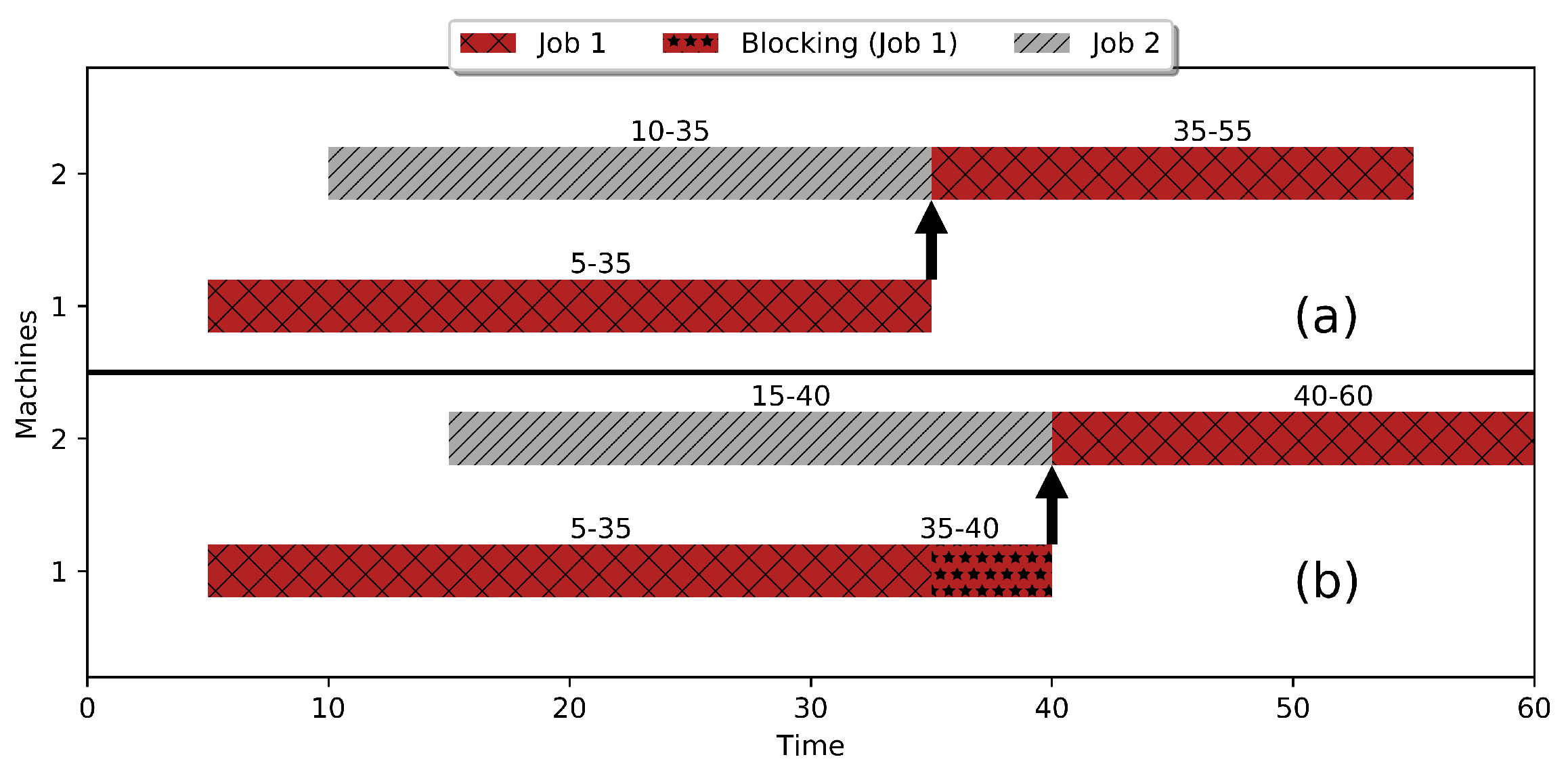
  • There are no buffers between machines, so jobs continue to occupy a machine after the end of an operation until the next machine is available.
One job of each type has to be completed per cycle. The objective is to minimise the cycle time. Until now, this has not considered the question of setup times.

2.1. Sequence-Dependent Setup Times

In the work by Panwalkar et al. [34] on task scheduling, it was found that 75% of problems occurring in practice required at least one setup which was dependent on the order of the execution of tasks. Moreover, in 15% of the problems, setup times between all pairs of tasks were required. In many real-world situations, such as those in the chemical, printing, pharmaceutical, and automobile industries, there may be several types of setup operations. For instance, between jobs, there can be cleaning or the changing of tools, and when considering a pair of jobs, there is a strong dependence on the preceding job. In the context of job shops, this type of setup is usually modelled as a sequence-dependent setup between jobs on the same machine.
In the literature, job-shop problems usually consist of two types of sequence-dependent setup times [35,36]. These are anticipatory setup times (AS) and nonanticipatory setup times (NS). For the case of AS, the setup can begin even if the job is not yet available to be processed but the machine that it is going to be processed on is idle, whereas for NS, the setup can begin only if both job and machine are available.
Due to blocking conditions often seen in limited or zero-buffered systems, we consider both types of setups separately in this research. Thereupon, in the case of AS, the setup must be done before loading the job when the corresponding machine is idle. Moreover, in the case of NS, the setup must be done only if both job and machine are available, and the job has been loaded on the machine. Figure 2 illustrates how anticipatory and nonanticipatory setups work with a small example.
Figure 3 shows the affect of setups on the CJSS with blocking conditions. Since there are no intermediate buffers between the machines, any job that completes an operation on a machine has to remain on the machine if the subsequent machine in its processing route is busy. However, if the subsequent machine is idle, the AS can commence on this machine before the job completes its operation on the current machine. The job can immediately move to the next machine after completing its operation. However, if the subsequent machine is busy and the job has completed its operation, the current machine gets blocked until the operation on that machine completes and also for AS. Figure 3 shows the differences of AS and NS, where AS affect the schedule by causing blocking conditions and NS occupy the machine before starting processing an operation.
To the best of the authors’ knowledge, the cyclic job-shop scheduling problem considering blocking conditions and sequence-dependent setup times at the same time have not been previously investigated in the literature.

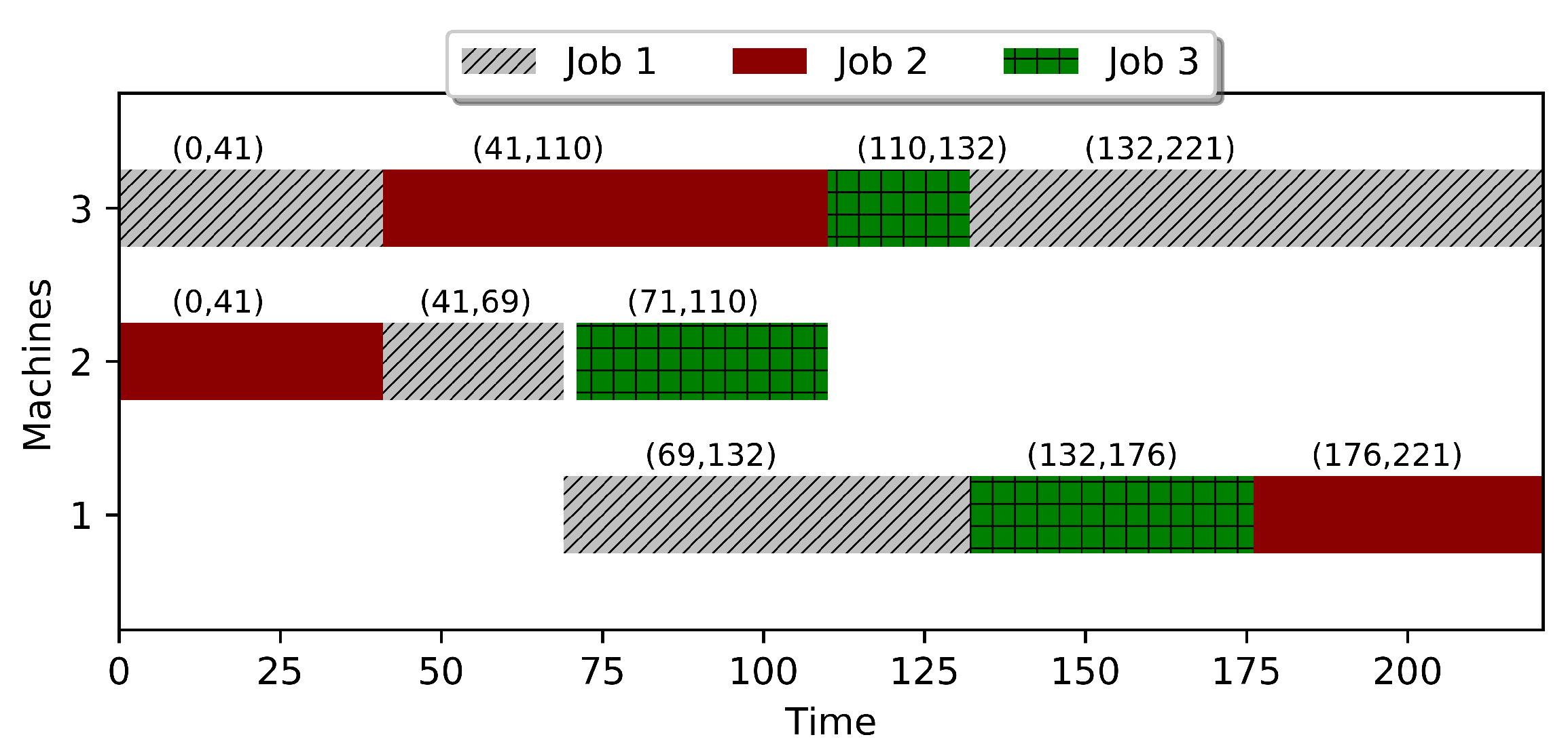
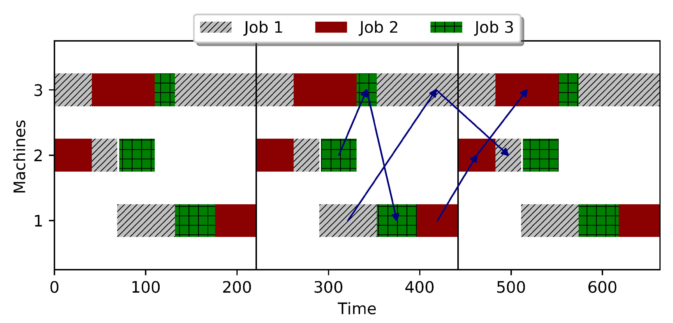
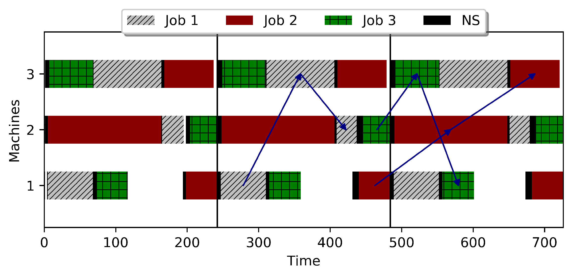
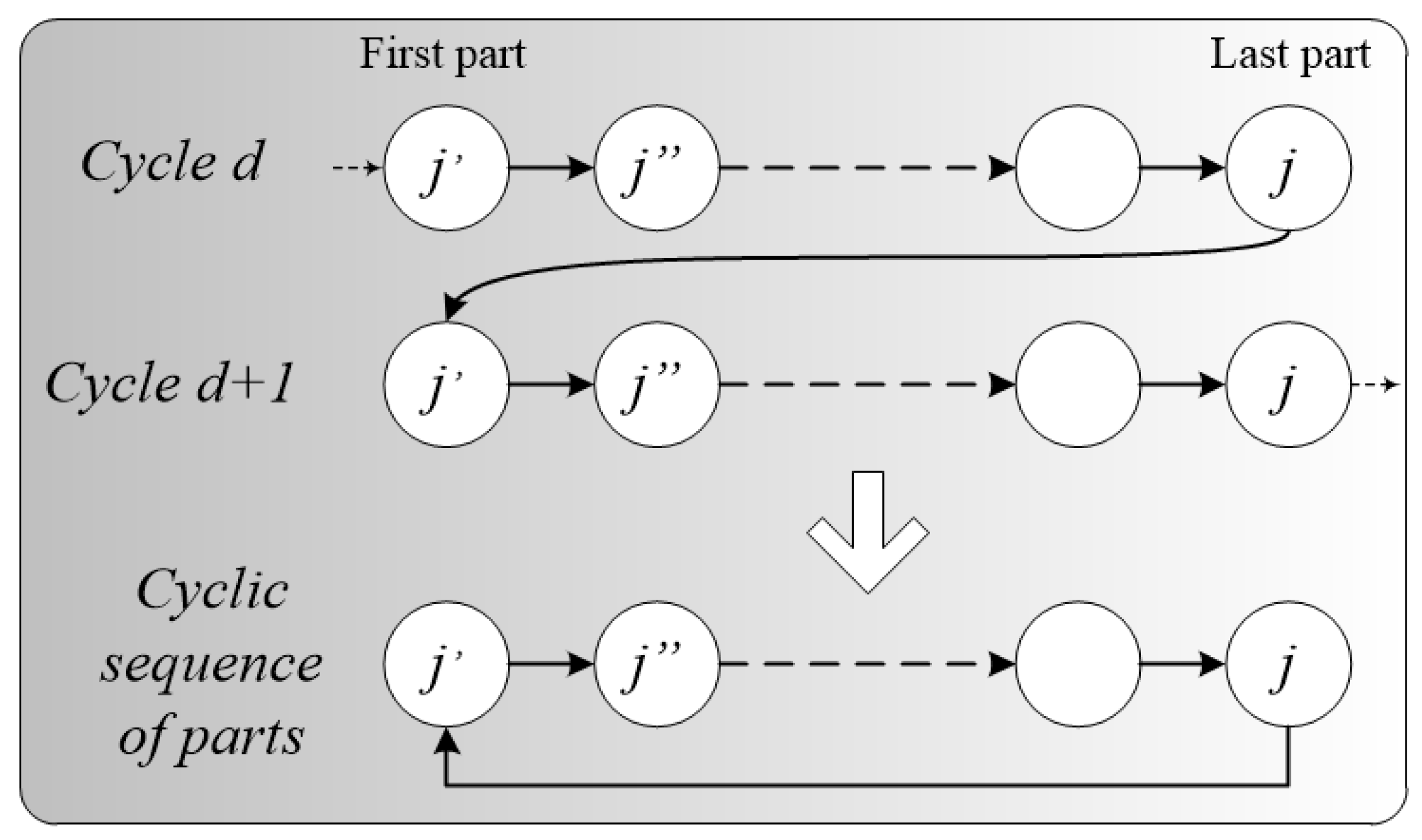
2.2. The Cyclic JSSP—An Example

We now provide a detailed example of the cyclic JSSP and work through a solution to the problem. We consider a test case, which consists of three machines and three jobs. Table 1 provides a breakdown of the related data including the sequence of machines that a job must be performed on and the associated processing times. Table 2 provides the sequence-dependent setup times between the jobs on each machine. For the purposes of comparing the AS and NS, we assume the A S j , j , m and N S j , j , m are equal.
Figure 4 provides an illustration of the optimal solution found for the example above without considering setups. The start time and departure time of all operations are detailed in the figure. In addition, Figure 5 demonstrates the three consecutive cycles of the problem instance within which the cyclic job-shop production is presented. A single MPS enters the production line in each cycle and the arrows indicate the processing route of the jobs from the same MPS. It also presents the route for each job through the cyclic schedule, which is a mapping to the classic blocking job-shop scheduling problem.
In similar fashion to the previous example, Figure 6 and Figure 7 show an optimal solution and three consecutive cycles, respectively, for the blocking CJSS problem with sequence-dependent anticipatory setups. The start time and departure time of all operations and sequence-dependent anticipatory setups are marked in black and are mentioned in the figure. We see three cycles associated with the optimal solution in Figure 7.
Again, Figure 8 and Figure 9 show examples of the optimal solution and three consecutive cycles, respectively, for the blocking CJSS problem with sequence-dependent nonanticipatory setups. The start time and departure time of all operations and required nonanticipatory sequence-dependent setup times are marked in black and are mentioned in the figure. We see three cycles associated with the optimal solution in Figure 9.

3. Mathematical Formulation of a Basic Model

In the following, we provide details of the mixed-integer linear programming (MILP) model for the basic cyclic job-shop scheduling (CJSS) problem without sequence-dependent setups. Due to the blocking conditions, the scheduling approach we used was based on the departure times of jobs from machines. The decision variables used in the proposed MILP model were:
X j , j , m 1 if job j immediately precedes job j on machine m; 0 otherwise;
R j , m 1 if machine m is occupied by job j at the beginning of a cycle; 0 otherwise;
B j , m 1 if job j is the first job to depart from machine m after the beginning of the cycle;
D j , i The departure time of job j from its i t h operation;
TThe cycle time;
U j , m An integer variable used to eliminate jobs’ sequence subtours on each machine m;
WA sufficiently large value, typically known as “Big M” in integer programming.
Note that the variable X determines the cyclic sequence of jobs on each machine. However, to do the scheduling of departure times, we need variables B to determine the first job on each machine. Similarly, R is used to capture the possibility that this first job has started processing before the start of the cycle so that the interval from the arrival of the part on the machine to the departure overlaps the cycle start time.

3.1. Occupied Machines Constraints

Scheduling all parts on all machines in a conceptual single cycle requires determining the occupied machines at the start of the cycle. Furthermore, based on the previously mentioned assumptions, each machine can process only one part at a time. The following constraint set (1) guarantees that each machine can be occupied by at most one part at the start time of the cycle.
j N R j , m 1 m M
We note that the occupied machines are determined in terms of the pressure of the processing constraints of parts and the operational constraints of machines that are presented in the following sections.

3.2. Processing Constraints of Each Part

In classic job-shop production systems, performing any operation on a part only starts after completing its previous operation. The CJSS problem can be considered to be a specific version of the classic problem. Consider that the i t h operation of part j is performed on machine m ( f i = m for part j), and if it is free at the beginning of the cycle, then the processing constraints are as follows:
D j , i 1 + P j , i D j , i
This states that the i t h operation of part j requires P j , i units of time to be elapsed. On the other hand, if machine m performing the i t h operation of part j is occupied at the beginning of the cycle by part j, then the related processing constraint would be as follows, due to the cyclic conditions:
D j , i 1 + P j , i D j , i + T
The binary variable R j , m is used to determine if the related machine m is occupied by part j at the start of the cycle. Hence, these processing restrictions can be formulated as constraints sets (4) and (5):
D j , o ( j , m ) 1 + P j , o ( j , m ) W R j , m D j , o ( j , m ) m M , j J m , 1 < o ( j , m )
D j , o ( j , m ) 1 + P j , o ( j , m ) D j , o ( j , m ) + T m M , j J m , 1 < o ( j , m )

3.3. Parts’ Sequence Determination on Machines

In addition, due to the cyclic scheduling, the relations between the cycles are established by the occupied machines at the start of the cycle. Actually, there is a cyclic sequence between the parts on each machine. To schedule the operations of all the parts in one cycle for each machine, the sequence of parts on each machine is considered to be determined based on the preceding and successor parts. The binary variable X determines the preceding and successor of all the parts on each machine. Thereupon, as illustrated in Figure 10, the first part in the next cycle is the successor of the last part in the present cycle.
To ensure the cyclic sequence of the parts, the following constraints sets (6)–(8) are used as follows:
j J m X j , j , m = 1 m M , j J m
U j , m U j , m + 1 J ( 1 X j , j , m ) m M , j j J m
The last of these constraints, (8), serves to eliminate the possibility of subtours in the sequence of parts [37].

3.4. Operational Constraints of Each Machine

The operational sequence constraints prevent the formation of conflicts in the usage of machines. Each machine should be unloaded before loading the next part on it and starting its processing operation. Figure 11 illustrates the operational sequence of parts on machines in the case where machine m is occupied or free at the start of the cycle.
To state the relation between the last and first parts of consecutive operations, the variable B is used. Variable B determines the first part that leaves each machine during the cycle time and the following constraints set (9) guarantees that each machine will have just one.
j J m B j , m = 1 m M
It is clear that if a machine is occupied by some part at the start of the cycle, then this part will be the first to depart, resulting in the following constraint set:
R j , m B j , m m M , j J m
Due to the operational sequence of parts on machines when the part j is the successor of part j on machine m then either
D j , i + P j , i D j , i or D j , i + P j , i D j , i + T .
The second inequality only holds for the case where j is the last part to depart from machine m before the end of the cycle and j departs at the start of the next cycle. The following constraints sets (12) and (13) are proposed based on these inequalities:
D j , o ( j , m ) + P j , o ( j , m ) M ^ ( 1 X j , j , m + B j , m ) D j , o ( j , m ) m M , j j J m
D j , o ( j , m ) + P j , o ( j , m ) D j , o ( j , m ) + T m M , j j J m
It should be also noted that in the case of a zero buffer between the machines, the completed parts have to remain on the machines until the machine for performing its next operation becomes available. If part j is the successor of part j on machine m then
D j , o ( j , m ) D j , o ( j , m ) 1 + T if machine m is idle at the start of the cycle with first job j D j , o ( j , m ) 1 otherwise
Note that the first case only arises if j departs m at the end of a cycle but part j does not arrive until the start of the next cycle. The constraints set (15) is formulated based on this inequality as follows:
D j , o ( j , m ) M ( 1 X j , j , m + B j m R j m ) D j , o ( j , m ) 1 m M , j j J m , 1 < o ( j , m )
This inequality holds if (a) j is after j on machine m so X j , j , m = 1 and (b) we do not have B j , m R j , m = 1 which would indicate that job j arrived after the start of the cycle.

3.5. Proposed Mathematical Programming Model

The proposed mathematical programming model is as follows:
[ M I P ] minimise T subject to C o n s t r a i n t s s e t s : ( 1 ) ( 15 ) T D j , o ( j , m ) m M , j J m X , R , B { 0 , 1 } T , D R + U R
In scheduling problems with buffers, safety times for the schedule need to be created and this increases the probability of a timely completion of the tasks. On the other hand, the problem described in this study assumes there is no buffer. In this respect, the number of feasible solutions decreases considerably, which increases the difficulty of the problem.

4. Blocking CJSS Problem with Sequence-Dependent Setup Times

We now extend the basic MIP formulation to incorporate the different types of setup times. Let A S j , j , m and N S j , j , m , respectively, denote the anticipatory and nonanticipatory sequence-dependent setup times (In the following sections AS refers to the anticipatory sequence-dependent setups, and NS refers to nonanticipatory sequence-dependent setups.) required on machine m where j is the successor job of j. The inequality Equation (11) was modified to Equation (16) for AS and Equation (17) for NS.
D j , i + A S j , j , m + P j , i D j , i or D j , i + A S j , j , m + P j , i D j , i + T
D j , i + N S j , j , m + P j , i D j , i or D j , i + N S j , j , m + P j , i D j , i + T

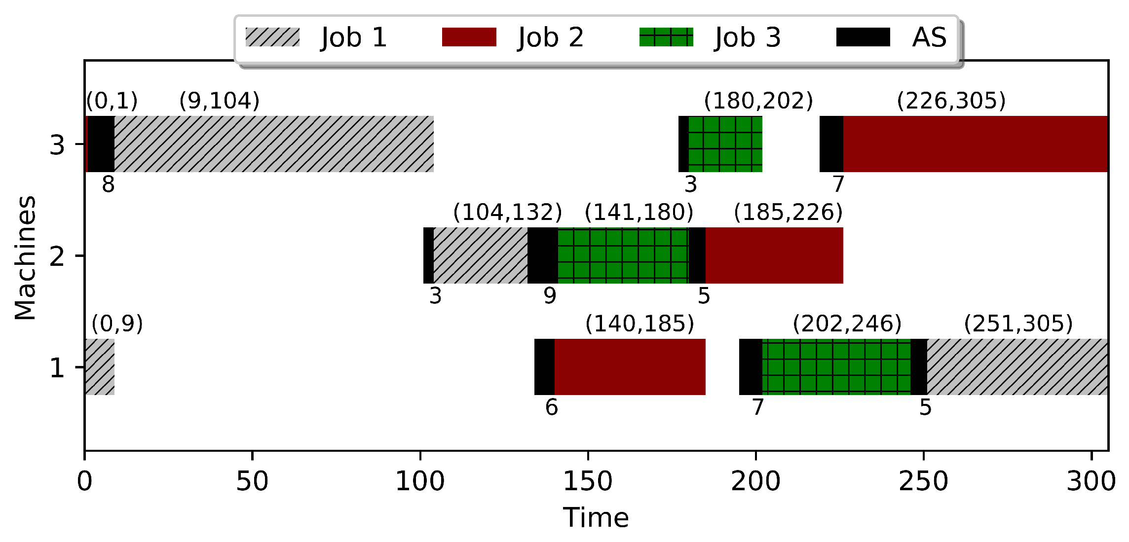
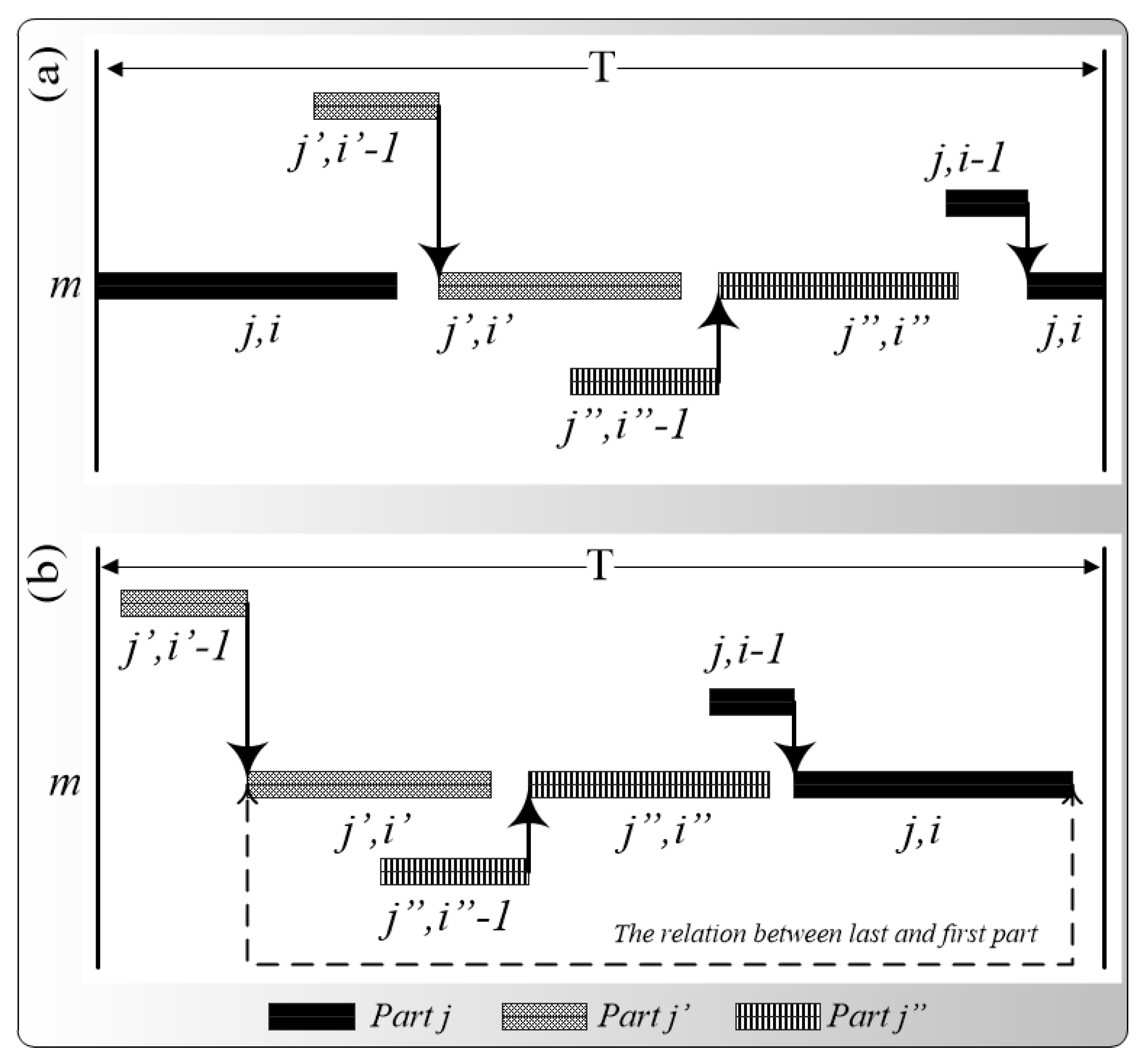
4.1. Blocking CJSS with Anticipatory Sequence-Dependent Setups (AS)

The MIP model was extended to consider AS. The constraints sets (12) and (13) were modified to (18) and (19) to ensure the operational sequence restrictions of jobs on machines based on the inequalities in Equation (16).
D j , o ( j , m ) + A S j , j , m + P j , o ( j , m ) M ^ ( 1 X j , j , m + B j , m ) D j , o ( j , m ) m M , j j J m
D j , o ( j , m ) + A S j , j , m + P j , o ( j , m ) D j , o ( j , m ) + T                                                             m M , j j J m
Additionally, a job cannot be loaded on the next machine before doing AS, even if both job and next machine are available. Therefore, as pointed in Figure 3, AS can cause blocking conditions. To ensure these restrictions, the inequalities in Equation (14) were modified as Equation (20).
D j , o ( j , m ) + A S j , j , m D j , o ( j , m ) 1 + T if machine m idle at start of cycle with first job j D j , o ( j , m ) 1 otherwise
Due to the inequalities in Equation (20), the constraints set (15) was also modified as follows.
D j , o ( j , m ) + A S j , j , m M ( 1 X j , j , m + B j m R j m ) D j , o ( j , m ) 1 m M , j j J m , 1 < o ( j , m )
The proposed mathematical programming model for the CJSS problem with sequence-dependent AS was extended as follows:
[ M I P A S ] minimise T subject to C o n s t r a i n t s s e t s : ( 1 ) ( 10 ) , ( 18 ) ( 21 ) T D j , o ( j , m ) m M , j J m X , R , B { 0 , 1 } T , D R + U R

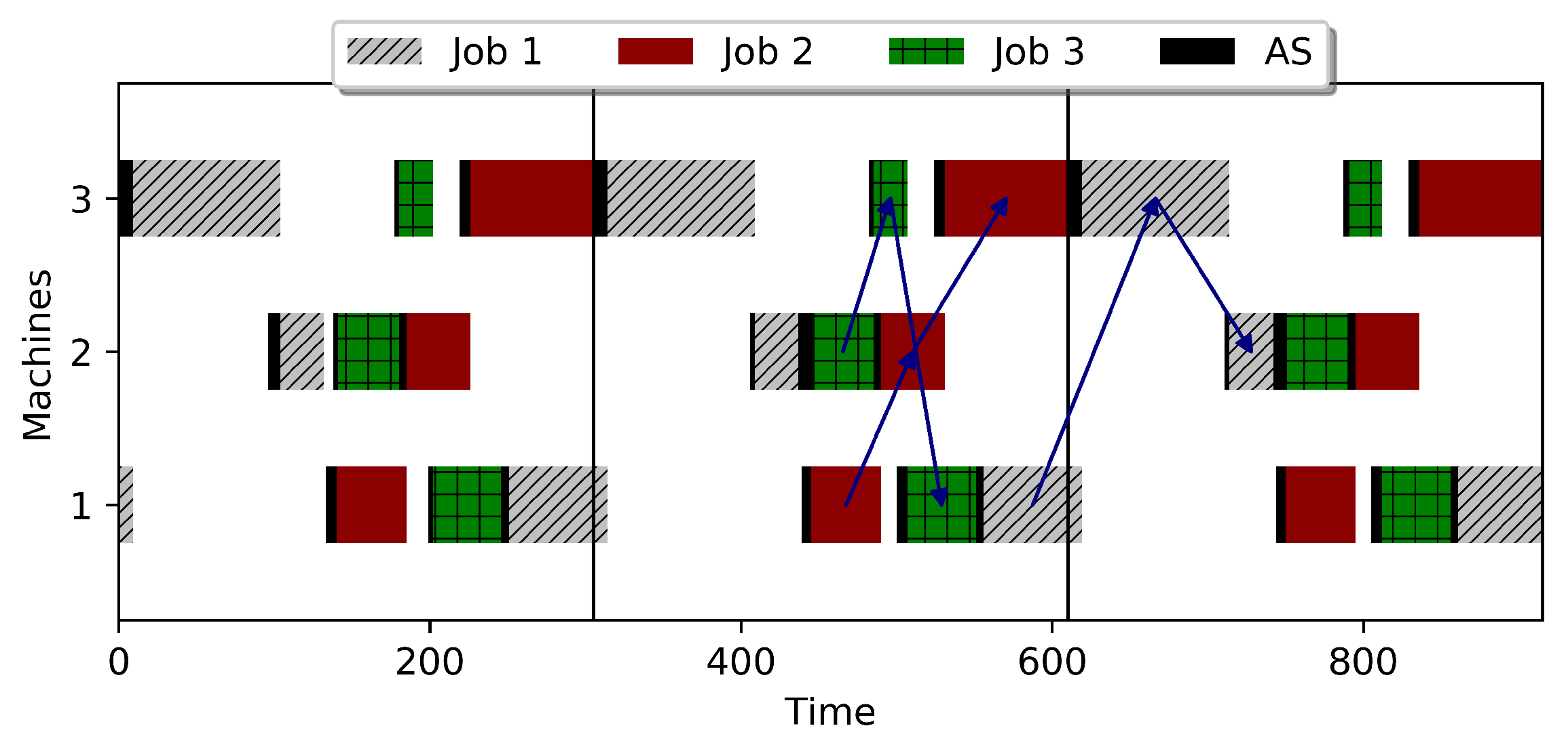
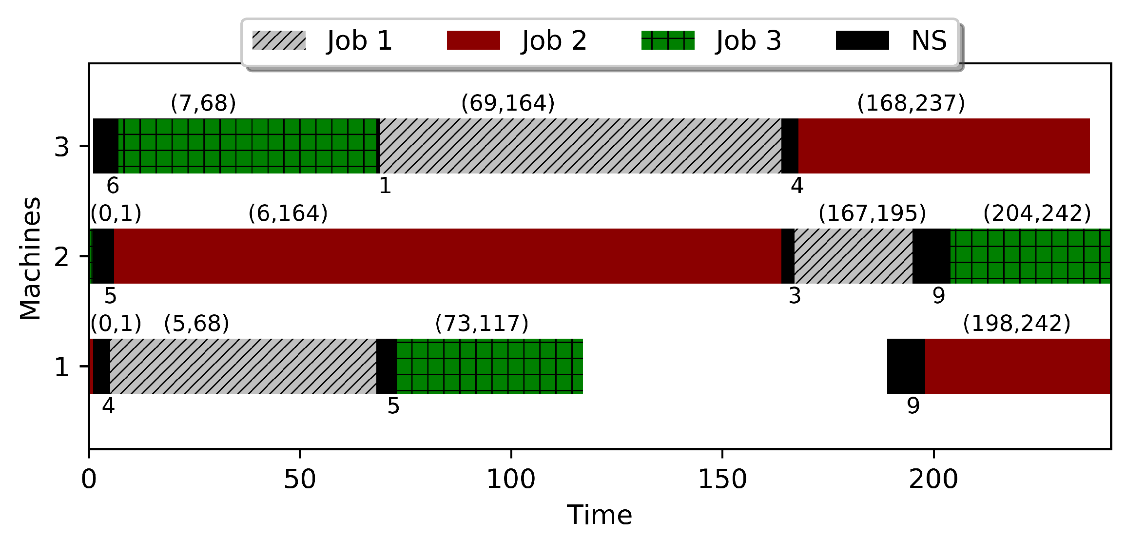
4.2. Blocking CJSS Problem with Nonanticipatory Sequence-Dependent Setups (NS)

As mentioned previously, NS need both the job and machine to be available. The constraints sets (12) and (13) were modified as follows to ensure that the operational sequence restrictions of jobs on machines according to the inequalities in Equation (17) in the nonanticipatory case.
D j , o ( j , m ) + N S j , j , m + P j , o ( j , m ) M ^ ( 1 X j , j , m + B j , m ) D j , o ( j , m ) m M , j j J m
D j , o ( j , m ) + N S j , j , m + P j , o ( j , m ) D j , o ( j , m ) + T                                                             m M , j j J m
Moreover, nonanticipatory setups directly affect the processing constraints as presented in Figure 2 for job j . The relationship between two consecutive operations of a job is stabilized considering the NS and processing time. NS need both the job and machine to be available, and hence, between two consecutive operations of a job there will be a time period to perform the NS. As a result, the NS directly affect the processing constraints. The inequalities in Equations (2) and (3) were presented for the case without any sequence-dependent setup times. To ensure these restrictions applied between two consecutive operations of a job in CJSS with NS, the inequalities in Equations (2) and (3) were extended to Equations (24) and (25).
D j , i 1 + N S j , j , m + P j , i D j , i
D j , i 1 + N S j , j , m + P j , i D j , i + T
where job j operates on machine m before job j, and N S j , j , m is the sequence-dependent NS. The variable R determined the occupying conditions, and hence, the processing constraints sets (4) and (5) were modified as constraints sets (26) and (27) based on Equations (24) and (25).
D j , o ( j , m ) 1 + X j , j , m × N S j , j , m + P j , o ( j , m ) W R j , m D j , o ( j , m ) m M , j j J m , 1 < o ( j , m )
D j , o ( j , m ) 1 + X j , j , m × N S j , j , m + P j , o ( j , m ) D j , o ( j , m ) + T                                                             m M , j j J m , 1 < o ( j , m )
Thus, the proposed MILP model for the CJSS problem with sequence-dependent nonanticipatory setups was extended as follows:
[ M I P N S ] minimise T subject to C o n s t r a i n t s s e t s : ( 1 ) , ( 6 ) ( 10 ) , ( 15 ) , ( 22 ) ( 27 ) T D j , o ( j , m ) m M , j J m X , R , B { 0 , 1 } T , D R + U R
The size of the basic formulation, as a function of an instance size with J jobs and K machines, is O ( J 2 K ) variables and O ( J 2 K ) constraints. The size is dominated by the X j , j , m variables with corresponding separation constraints (12)–(15) for each such X variable. The anticipatory and nonanticipatory variants simply modify the separation constraints but add neither new variables nor additional constraints.

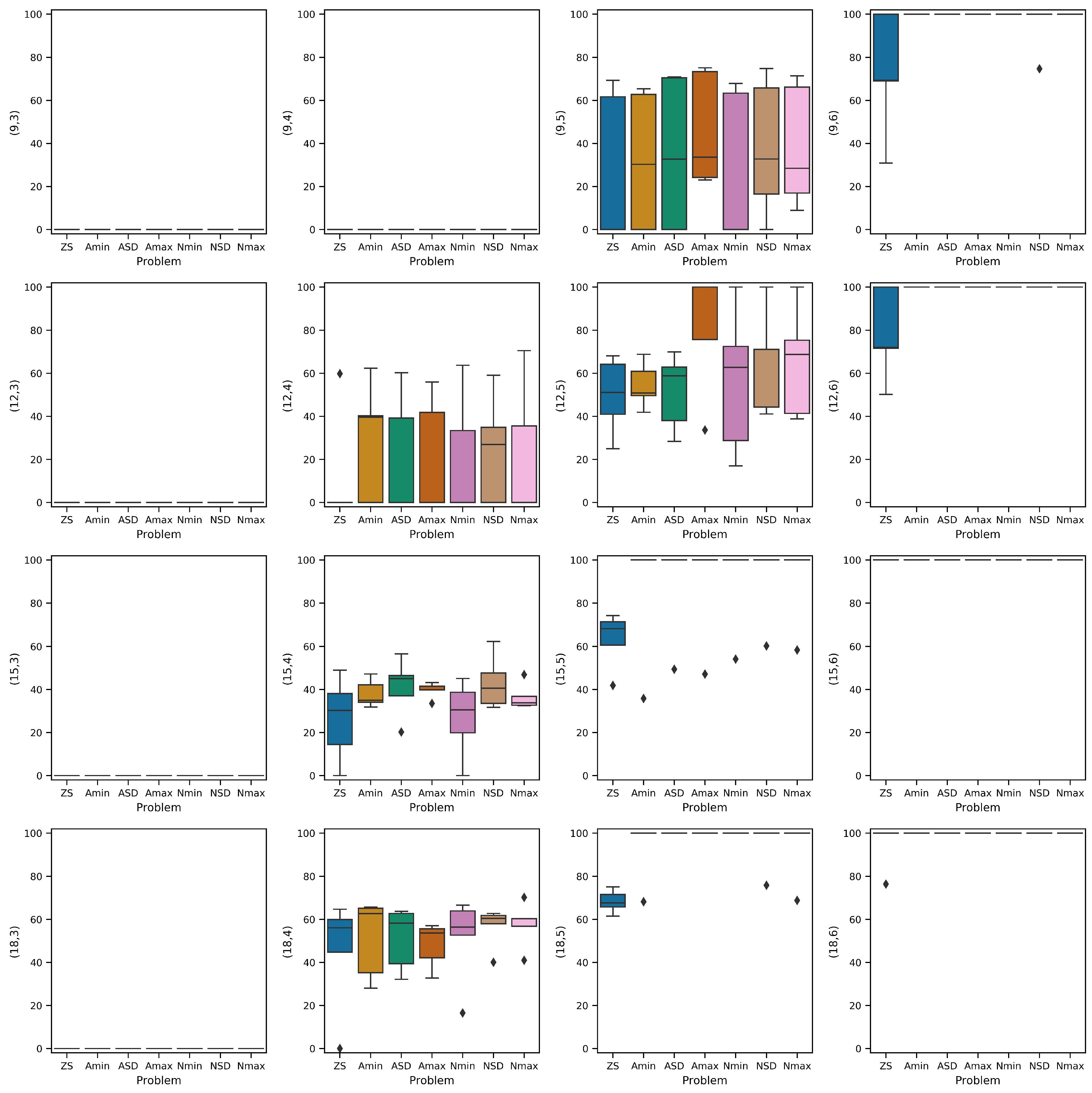
5. Experimental Settings and Results

In the literature, there is no benchmark dataset specifically designed for the cyclic JSS problem. Cyclic production systems have minimal part sets, which makes the problem significantly different to classic JSS. This leads to two major differences. First, the objective of the classic JSS is minimising the makespan, compared to cycle time in cyclic JSS. While both objectives have similarities, the resulting (optimal) schedules can be substantially different. Second, in the cyclic problem, there is less variety among the products but higher volumes relative to classic job shops. This leads to the size of the minimal part sets in cyclic JSS being smaller than the number of jobs in classic JSS. Due to the above reasons, for this study, we designed a number of benchmark problem instances (see Appendix A, which provides details of the algorithm for generating the instances) motivated by practical requirements and using typical characteristics seen in JSS.
The MIPs developed in this study were programmed in Python 3.6 and all experiments were conducted on MonARCH, the campus cluster at Monash University. Each run was given four cores and a limit of 10 GB memory. The MIP models were solved using Gurobi 9.0.1 (http://www.gurobi.com/ (accessed on 30 August 2022)). Each run was given one hour of execution time.
Table 3 shows the results of the MIP models for the blocking CJSS problem without setups, with sequence-dependent anticipatory and nonanticipatory setups. There were 16 problem instances with different combinations of machines (K) and jobs (J), which were generated by the method described above. The results were split in three jobs: (1) cyclic job shop without sequence-dependent setups, (2) cyclic job shop with anticipatory sequence-dependent setups, and (3) cyclic job shop with nonanticipatory sequence-dependent setups. For each MIP, the details provided include the number of constraints (#Cons), number of variables (#Vars), the objective value of the best feasible solution (BF), the lower bound (LB), the gap between the upper and lower bounds G a p = ( B F L B ) L B , and the total time taken. If no feasible solution was found, the corresponding BF and Gap columns have a dash (-).
First, we considered cyclic JSS on its own. We see that for problems with a small number of jobs (three) the optimal solution was always found, and the time required was often quite small (under 30 s) relative to the time limit. Additionally, for a small number of machines (9, 12) and four jobs, the optimal solutions could also be found. For a larger number of jobs (five), feasible solutions were found but often with large gaps. For problems with six jobs, no feasible solutions were found irrespective of the number of machines. Nonetheless, the MIP always found lower bounds (the quality of which could not be guaranteed).
Considering cyclic JSS with anticipatory setups, we see a similar pattern. However, in this case, the problems proved more difficult to solve with one more problem not being solved (18 machines and 5 jobs) compared to Cyclic JSS. Additionally, when solutions were found, if they were not optimal, the gaps were larger. This is not surprising, since the overhead of the anticipatory setup times makes the problem more complex.
Finally, considering cyclic JSS with nonanticipatory setups, we see that it became even harder (compared to cyclic JSS and cyclic JSS with AS) to find solutions within the allowed time limits. The nonanticipatory setup required a job moving between machines to immediately leave the machine that it was currently on, and this meant that the MIP model struggled more when attempting to find a feasible solution.
In order to further understand the impact of sequence-dependent setup times, we considered a constant setup time with the following two options: (a) MIN: use the minimum set up time in a problem instance as the standard setup time between all jobs and (b) MAX: use the maximum set up time in a problem instance as the standard setup time between all jobs. Furthermore, to account for random effects in the data, four different datasets were generated with the same problem sizes. Table 4 shows the results of the comparisons with these changes for five different datasets for each problem size. The first three columns show replication (Rep), machines (K), and jobs (J), and the following columns are split by the best feasible solution, lower bounds, and gaps. Within each, the results are split by the type of setup, i.e., no setups (ZS), anticipatory, and nonanticipatory. For the case with setups, the results are further split by sequence-dependent setups (SD), standard maximum setups (MAX), and standard minimum setups (MIN).
The results showed, as expected, that cycle times increased with increasing amounts of setup time. Furthermore, the MIP models for which setups were used led to more instances where solutions could not be found. For example, MAX compared to ZS clearly showed two instances where solutions were not found. Interestingly, MIN was able to find two solutions where no solution was found in the case of ZS.
The differences in cycle times in the systems with sequence-dependent and standard setups demonstrated the importance of considering the sequence-dependent setups in blocking cyclic job-shop systems. Moreover, the cycle times of problems with no setups and minimum nonanticipatory setups were very similar, whereas the minimum anticipatory setups were rather different. In previous sections, we discussed that anticipatory setups could cause blocking conditions on the machines. Table 4 demonstrates that the cycle times were smaller in the systems with nonanticipatory setups comparing to the systems with anticipatory setups. These points present the importance of anticipatory setups in blocking job-shop systems.
Figure 12 presents the performance of the proposed MIP modelling approach for CJSS and demonstrates the Gap for different size of test instances. The plots demonstrate that the proposed approach was able to solve all the instances with a small number of jobs (solved optimally or close to optimality) and show that it was an efficient approach for cyclic production systems with fewer product varieties. Moreover, the MIP approach could find solutions for the medium-size test instances with four jobs (considering all machine) and five jobs (with 9 and 12 machines) but struggled to prove optimality. For instances with a large number of jobs and machines, the MIP approach rarely found solutions (plots on the right of the figure). The plots for the instances with five jobs indicate that the complexity of CJSS problem with maximum anticipatory setup (Amax) was higher compared to that of the CJSS problem with maximum nonanticipatory setup (Nmax). Overall, Figure 12 shows that the MIP approach could be used efficiently in production systems with a lower range of product varieties.

6. Conclusions

The cyclic job-shop scheduling problem was investigated in this paper. A novel mixed-integer programming model was proposed for the problem based on the characteristics of cyclic scheduling. Thereupon, the operations were scheduled within a single cycle. The occupying machines at the start time of the cycle had an important effect on solution quality due to the characteristics of the job-shop problem. Technological manufacturing cells, such as robotic cells, were attempted in order to eliminate or decrease the number of buffers. Thereupon, manufacturing systems without buffers were encountered in real situations. This study investigated the problem where the machines had no buffers that caused the blocking conditions, which rapidly decreased the number of feasible solutions and, therefore, made it a lot harder to find those feasible solutions.
Moreover, the sequence-dependent setups were considered in this research. There were two types of setups, anticipatory and nonanticipatory, which were included before and after loading the jobs on the machines, respectively. Thereupon, the anticipatory and nonanticipatory sequence-dependent setups were investigated in this research separately. The advantages of this study and the achievements can be outlined as follows:
  • Previous studies on modelling the cyclic job-shop scheduling problem were based on performing operations in iterative cycles, whereas the proposed model in this research scheduled all the operations within a single cycle.
  • Due to the scheduling within a single cycle, the proposed model could be simply extended to different resource constrained variants.
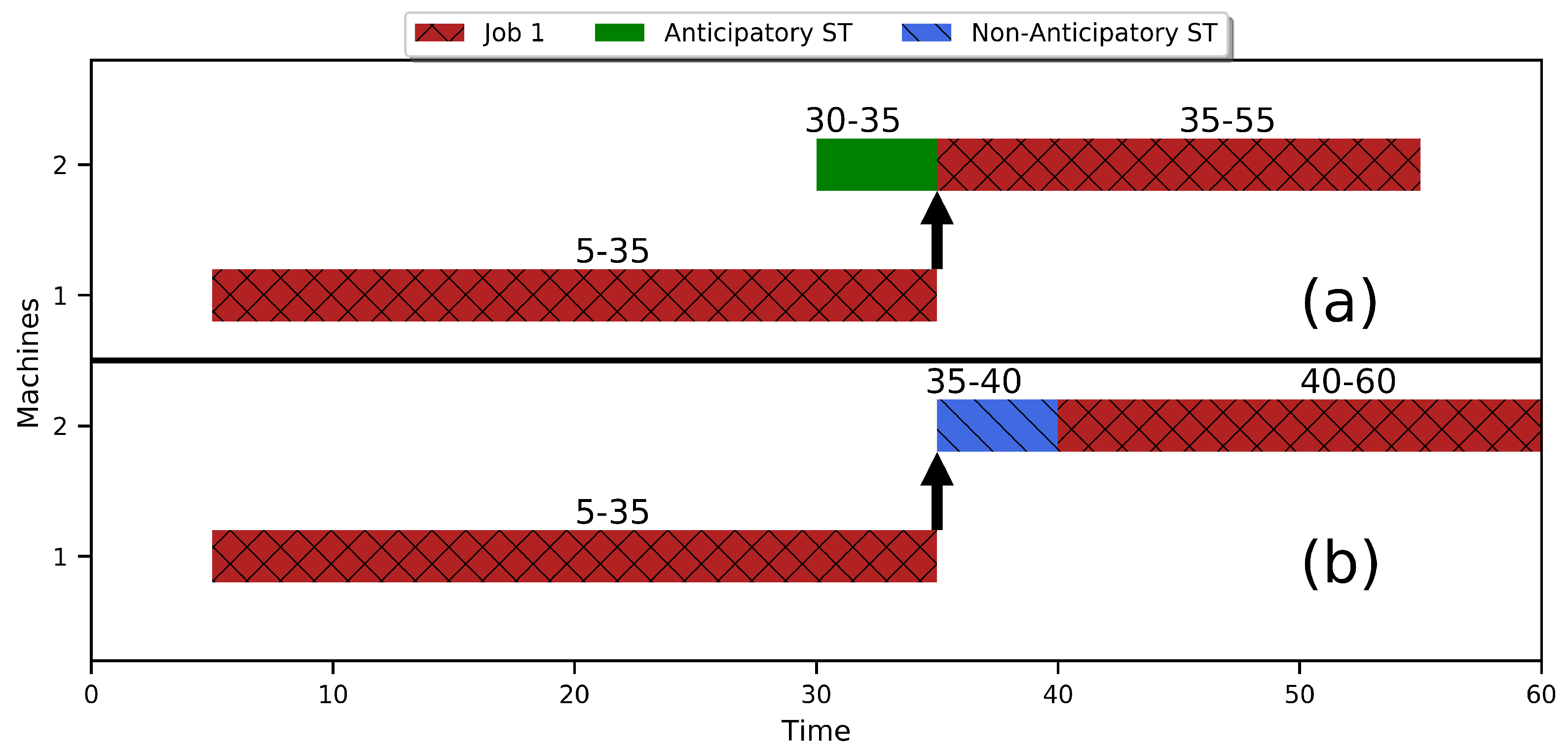
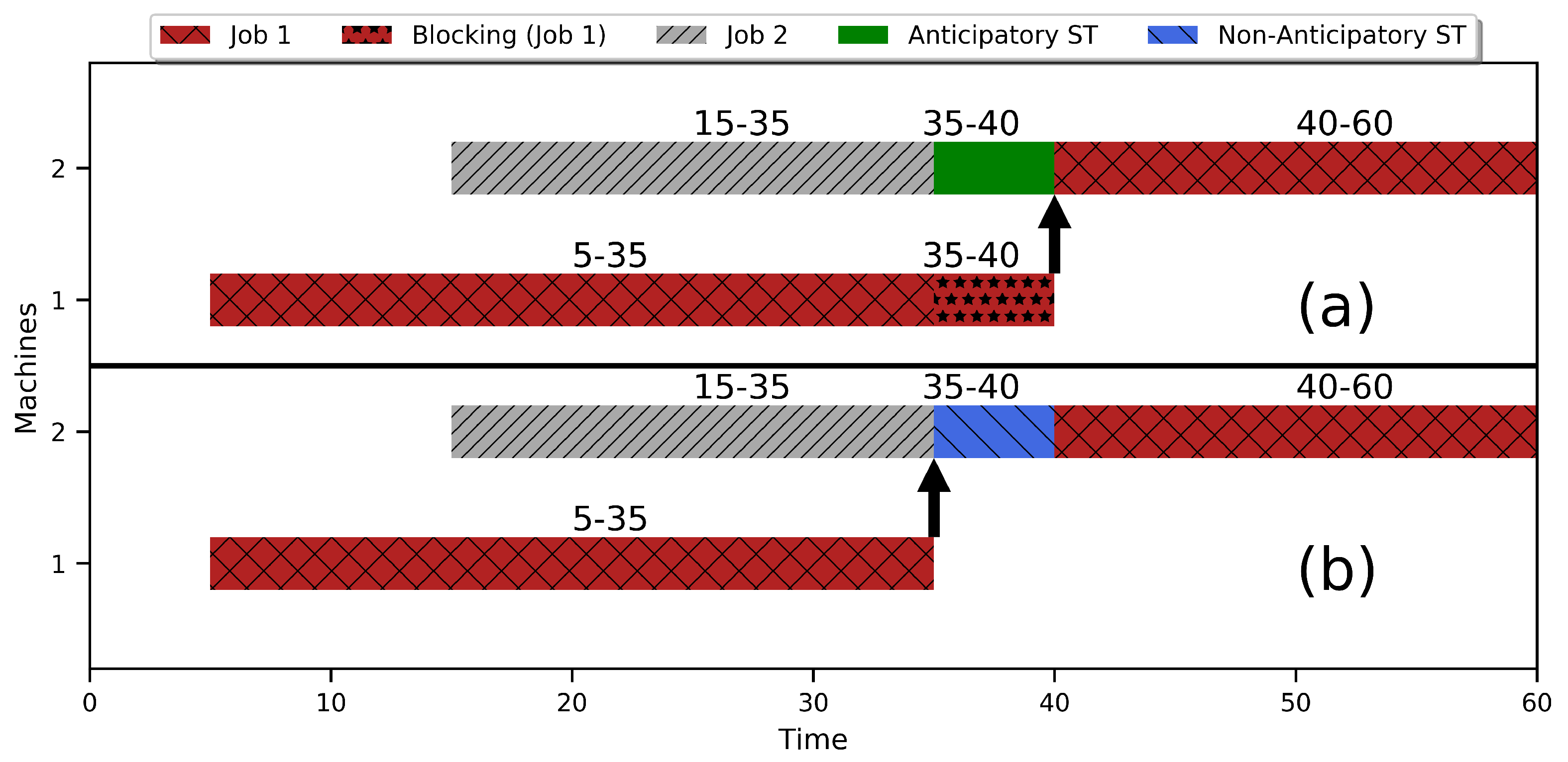
  • Two kinds of sequence-dependent setups were considered based on anticipatory and nonanticipatory concepts.
  • The nonanticipatory setups did not affect the blocking condition as the related job did not have to wait for the previous machine because of the related setup.
  • The anticipatory setups directly affected the blocking conditions, as any part might need to wait on the previous machine until the related setup was completed.
As future research, the proposed model could be applied to cyclic job-shop robotic cells. Moreover, this research could be extended to manufacturing systems with servers performing the setups.
The difficulty of solving these problems with MIP solvers observed in this paper indicate that further research on exact methods is required, perhaps based on decomposition methods, in order to solve large-scale cyclic job-shop scheduling problems. Moreover, the proposed model could be applied to cyclic job-shop scheduling problems in resource-constrained systems where robotic cells and servers perform the setups.

Author Contributions

Conceptualization, A.E.; Data curation, A.E.; Investigation, A.E., D.R.T. and A.T.E.; Methodology, A.E., D.R.T. and A.T.E.; Software, A.E.; Validation, A.E. and D.R.T.; Visualization, A.E.; Writing—original draft, A.E. and D.R.T.; Writing—review & editing, A.E., D.R.T. and A.T.E. All authors have read and agreed to the published version of the manuscript.

Funding

This research received no external funding.

Institutional Review Board Statement

Not applicable.

Informed Consent Statement

Not applicable.

Data Availability Statement

Not applicable.

Conflicts of Interest

The authors declare no conflict of interest.

Appendix A. Generating Problem Instances

Algorithm A1 was used to generate the test problems for each benchmark with a specific number of jobs and machines based on the benchmark generation method reported by Taillard [38]. The procedure starts by taking as input the number of jobs, number of machines, the ranges for processing times, and sequence-dependent setup times. Lines 2–5 set lists for recording the processing route of each job. The processing time of each operation of each job is randomly generated within lines 6–7. Lines 8–9 generate the required sequence-dependent setup times between each pair of jobs. This is followed by generating the processing route for each job in lines 10–15, where the list Ψ has the set of machines that each job should be processed on. For each operation (line 12), a machine is selected from the set of machines and then Ψ is updated by eliminating the selected machine. Finally, a machine from the set of remaining machines is selected for the next operation in the queue.
  • The operation times of jobs on the machines are generated from the uniform distribution [ a , b ] = [ 1 , 99 ] .
  • The sequence-dependent setup times are generated from the uniform distribution [ a , c ] = [ 1 , 33 ] .
  • The standard maximum and minimum setup times are equal to the maximum and minimum of sequence-dependent setup times, respectively.
Algorithm A1 Generate Problems.
1:
procedureFunction( J , K , a , b , c )
2:
    for  j { 1 , , J }  do
3:
         O j K
4:
         I j { 1 , , O j }
5:
         F j = { }
6:
    for  ( j , i ) : j { 1 , , J } , i I j  do
7:
         P j , i U [ a , b ]
8:
    for  ( j , j , m ) : j , j { 1 , , J } , j j , m { 1 , , K }  do
9:
         A S j , j , m = N S j , j , m U [ a , c ]
10:
    for  j : j { 1 , , J }  do
11:
         Ψ = { 1 , , K }
12:
        for  i : i I j  do
13:
            f i randomly select from Ψ
14:
            Ψ Ψ f i
15:
            F j F j f i
16:
    return  ( P , A S , N S , I j , F j )

References

  1. Brucker, P.; Kampmeyer, T. Tabu search algorithms for cyclic machine scheduling problems. J. Sched. 2005, 8, 303–322. [Google Scholar] [CrossRef]
  2. Hanen, C. Study of a NP-hard cyclic scheduling problem: The recurrent job-shop. Eur. J. Oper. Res. 1994, 72, 82–101. [Google Scholar] [CrossRef]
  3. Brucker, P. Multiprocessor tasks. In Scheduling Algorithms; Springer: Berlin/Heidelberg, Germany, 2001; pp. 313–341. [Google Scholar]
  4. Wójcik, R.; Pempera, J. Designing cyclic schedules for streaming repetitive job-shop manufacturing systems with blocking and no-wait constraints. IFAC-PapersOnLine 2019, 52, 73–78. [Google Scholar] [CrossRef]
  5. Levner, E.; Kats, V.; De Pablo, D.A.L.; Cheng, T.E. Complexity of cyclic scheduling problems: A state-of-the-art survey. Comput. Ind. Eng. 2010, 59, 352–361. [Google Scholar]
  6. Šůcha, P.; Hanzálek, Z. A cyclic scheduling problem with an undetermined number of parallel identical processors. Comput. Optim. Appl. 2011, 48, 71–90. [Google Scholar] [CrossRef]
  7. Brauner, N.; Finke, G.; Kubiak, W. Complexity of one-cycle robotic flow-shops. J. Sched. 2003, 6, 355–372. [Google Scholar] [CrossRef]
  8. Lee, T.E.; Seo, J. Stochastic cyclic flow lines: Non-blocking, Markovian models. J. Oper. Res. Soc. 1998, 49, 537–548. [Google Scholar] [CrossRef]
  9. Xing, L.N.; Chen, Y.W.; Yang, K.W. Multi-population interactive coevolutionary algorithm for flexible job shop scheduling problems. Comput. Optim. Appl. 2011, 48, 139–155. [Google Scholar] [CrossRef]
  10. Grabowski, J.; Pempera, J. Sequencing of jobs in some production system. Eur. J. Oper. Res. 2000, 125, 535–550. [Google Scholar] [CrossRef]
  11. Ronconi, D.P. A note on constructive heuristics for the flowshop problem with blocking. Int. J. Prod. Econ. 2004, 87, 39–48. [Google Scholar] [CrossRef]
  12. Gong, H.; Tang, L.; Duin, C. A two-stage flow shop scheduling problem on a batching machine and a discrete machine with blocking and shared setup times. Comput. Oper. Res. 2010, 37, 960–969. [Google Scholar] [CrossRef]
  13. Martinez, S.; Dauzère-Pérès, S.; Gueret, C.; Mati, Y.; Sauer, N. Complexity of flowshop scheduling problems with a new blocking constraint. Eur. J. Oper. Res. 2006, 169, 855–864. [Google Scholar] [CrossRef]
  14. Lange, J.; Werner, F. Approaches to modeling train scheduling problems as job-shop problems with blocking constraints. J. Sched. 2018, 21, 191–207. [Google Scholar] [CrossRef]
  15. Kats, V.; Levner, E. Cyclic scheduling in a robotic production line. J. Sched. 2002, 5, 23–41. [Google Scholar] [CrossRef]
  16. Dawande, M.W.; Geismar, H.N.; Sethi, S.P.; Sriskandarajah, C. Throughput Optimization in Robotic Cells; Springer Science & Business Media: Berlin/Heidelberg, Germany, 2007; Volume 101. [Google Scholar]
  17. Ayala, M.; Benabid, A.; Artigues, C.; Hanen, C. The resource-constrained modulo scheduling problem: An experimental study. Comput. Optim. Appl. 2013, 54, 645–673. [Google Scholar] [CrossRef] [Green Version]
  18. Pempera, J.; Smutnicki, C. Open shop cyclic scheduling. Eur. J. Oper. Res. 2018, 269, 773–781. [Google Scholar] [CrossRef]
  19. Wang, J.; Pan, C.; Hu, H.; Li, L.; Zhou, Y. A cyclic scheduling approach to single-arm cluster tools with multiple wafer types and residency time constraints. IEEE Trans. Autom. Sci. Eng. 2018, 16, 1373–1386. [Google Scholar] [CrossRef]
  20. Elmi, A.; Nazari, A.; Thiruvady, D.; Durmusoglu, A. Cyclic Flow Shop Robotic Cell Scheduling Problem With Multiple Part Types. IEEE Trans. Eng. Manag. 2020. [Google Scholar] [CrossRef]
  21. Bożejko, W.; Uchroński, M.; Wodecki, M. Block approach to the cyclic flow shop scheduling. Comput. Ind. Eng. 2015, 81, 158–166. [Google Scholar] [CrossRef]
  22. Brucker, P.; Kampmeyer, T. Cyclic job shop scheduling problems with blocking. Ann. Oper. Res. 2008, 159, 161–181. [Google Scholar] [CrossRef]
  23. Song, J.S.; Lee, T.E. Petri net modeling and scheduling for cyclic job shops with blocking. Comput. Ind. Eng. 1998, 34, 281–295. [Google Scholar] [CrossRef]
  24. Cavory, G.; Dupas, R.; Goncalves, G. A genetic approach to solving the problem of cyclic job shop scheduling with linear constraints. Eur. J. Oper. Res. 2005, 161, 73–85. [Google Scholar] [CrossRef]
  25. Kechadi, M.T.; Low, K.S.; Goncalves, G. Recurrent neural network approach for cyclic job shop scheduling problem. J. Manuf. Syst. 2013, 32, 689–699. [Google Scholar] [CrossRef] [Green Version]
  26. Kampmeyer, T. Cyclic Scheduling Problems. Ph.D. Thesis, Universität Osnabrück, Osnabrück, Germany, 2006. [Google Scholar]
  27. Brucker, P.; Kampmeyer, T. A general model for cyclic machine scheduling problems. Discret. Appl. Math. 2008, 156, 2561–2572. [Google Scholar] [CrossRef] [Green Version]
  28. Brucker, P.; Burke, E.K.; Groenemeyer, S. A mixed integer programming model for the cyclic job-shop problem with transportation. Discret. Appl. Math. 2012, 160, 1924–1935. [Google Scholar] [CrossRef] [Green Version]
  29. Brucker, P.; Burke, E.K.; Groenemeyer, S. A branch and bound algorithm for the cyclic job-shop problem with transportation. Comput. Oper. Res. 2012, 39, 3200–3214. [Google Scholar] [CrossRef]
  30. Quinton, F.; Hamaz, I.; Houssin, L. A mixed integer linear programming modelling for the flexible cyclic jobshop problem. Ann. Oper. Res. 2020, 285, 335–352. [Google Scholar] [CrossRef] [Green Version]
  31. Gultekin, H.; Dalgıç, Ö.O.; Akturk, M.S. Pure cycles in two-machine dual-gripper robotic cells. Robot. Comput.-Integr. Manuf. 2017, 48, 121–131. [Google Scholar] [CrossRef] [Green Version]
  32. Ghadiri Nejad, M.; Shavarani, S.M.; Güden, H.; Barenji, R.V. Process sequencing for a pick-and-place robot in a real-life flexible robotic cell. Int. J. Adv. Manuf. Technol. 2019, 103, 3613–3627. [Google Scholar] [CrossRef]
  33. Foumani, M.; Razeghi, A.; Smith-Miles, K. Stochastic optimization of two-machine flow shop robotic cells with controllable inspection times: From theory toward practice. Robot. Comput.-Integr. Manuf. 2020, 61, 101822. [Google Scholar] [CrossRef]
  34. Panwalkar, S.; Dudek, R.; Smith, M. Sequencing research and the industrial scheduling problem. In Proceedings of the Symposium on the Theory of Scheduling and Its Applications; Springer: Berlin/Heidelberg, Germany, 1973; pp. 29–38. [Google Scholar]
  35. Defersha, F.M.; Chen, M. A parallel genetic algorithm for a flexible job-shop scheduling problem with sequence dependent setups. Int. J. Adv. Manuf. Technol. 2010, 49, 263–279. [Google Scholar] [CrossRef]
  36. Framinan, J.M.; Leisten, R.; García, R.R. Manufacturing scheduling systems. In An integrated view on Models, Methods and Tools; Springer: Berlin/Heidelberg, Germany, 2014; pp. 51–63. [Google Scholar]
  37. Miller, C.E.; Tucker, A.W.; Zemlin, R.A. Integer programming formulation of traveling salesman problems. J. ACM (JACM) 1960, 7, 326–329. [Google Scholar] [CrossRef]
  38. Taillard, E. Benchmarks for basic scheduling problems. Eur. J. Oper. Res. 1993, 64, 278–285. [Google Scholar] [CrossRef]
Figure 1. Blocking conditions in job-shop scheduling.
Algorithms 15 00375 g001
Figure 2. The anticipatory (a) and nonanticipatory (b) setups to process a job on a machine.
Algorithms 15 00375 g002
Figure 3. The effects of anticipatory (a) and nonanticipatory (b) setups on the schedule.
Algorithms 15 00375 g003
Figure 4. The optimal solution for the problem instance in Table 1; blocking CJSS problem.
Algorithms 15 00375 g004
Figure 5. The Gantt chart of three consecutive cycles for the problem instance in Table 1; blocking CJSS problem.
Algorithms 15 00375 g005
Figure 6. The detailed Gantt chart of the optimal solution found for the instance problem; blocking CJSS problem with sequence-dependent anticipatory setups (AS).
Algorithms 15 00375 g006
Figure 7. The Gantt chart of three consecutive cycles for the considered instance problem; blocking CJSS problem with sequence-dependent anticipatory setups (AS).
Algorithms 15 00375 g007
Figure 8. The detailed Gantt chart of the optimal solution found for the instance problem; blocking CJSS problem with sequence-dependent nonanticipatory setups (NS).
Algorithms 15 00375 g008
Figure 9. The Gantt chart of three consecutive cycles for the considered instance problem; blocking CJSS problem with sequence-dependent nonanticipatory setups (NS).
Algorithms 15 00375 g009
Figure 10. The cyclic sequence of parts on any machine.
Algorithms 15 00375 g010
Figure 11. The operational sequencing restrictions of any machine m; (a,b) presents the restriction when m is occupied and free at the start of the cycle, respectively.
Algorithms 15 00375 g011
Figure 12. Box plots of the gaps in Table 4 (with J = 3 , , 6 for the four columns and K = 9 , 12 , 15 , 18 for the rows of graphs).
Algorithms 15 00375 g012
Table 1. The machine and processing time of each operation of the jobs.
JobsMachinesProcessing Times
1132639528
2123454169
3231392244
Table 2. The sequence-dependent setup times between the pair of jobs on each machine.
Machines
123
Jobs123123123
1165779743
2477383816
3594553176
Table 3. The performance of proposed MIP approaches on the test problem instances (#Cons: number of constraints; #Var: number of variables; BF: best found; LB: lower bound).
KJ #Cons #Var Cyclic JSS: Zero Setups Anticipatory Setups Nonanticipatory Setups
BFLBGapTimeBFLBGapTimeBFLBGapTime
9373319025725707.35390390018.6337337017.3
4131328927027005.0944144106.9233533507.77
5215740653516469.27360070120770.42360066016674.803600
6331954156639130.923600-444-3600-437-3600
123988253258258014.94373373014.53354354022.83
417693853353350308.594684680684.564314310386.49
5290454152918964.21360069525862.88360074121471.083600
64465721-190-3600-223-3600-206-3600
1531243316313313011.0744944909.15411411018.75
4222548134421338.08360045725144.99360046224247.623600
5365167656833041.90360076138549.413600-285-3600
65611901-171-3600-200-3600-195-3600
1831498379275275017.42365365026.56360360026.95
4268157736420144.78360051931539.36360048418062.763600
5439881160017171.553600-210-360072117575.793600
667571081-184-3600-198-3600-193-3600
Table 4. A comparison of cycle times of different anticipatory and nonanticipatory setups for five repetitions of all MIP models. ZS: zero setups, SD: sequence-dependent, Max: standard maximum setup, Min: standard minimum setup.
Rep K J Best Found Lower Bound Gap
ZS Anticipatory Nonanticipatory ZS Anticipatory Nonanticipatory ZS Anticipatory Nonanticipatory
Min SD Max Min SD Max Min SD Max Min SD Max Min SD Max Min SD Max
1932573143904642623374172573143904642623374170000000
42703654415262753354472703654415262753354470000000
553552470195454666081316419520723817516623269.2762.7370.4275.0967.8974.8071.43
6566------39139744458339743758330.92------
1232583163734462643544332583163734462643544330000000
43353934685593404315233353934685593404315230000000
5529527695-50874199018920625816618921424464.2160.9262.88-62.7371.0875.34
6-------190205223211182206245-------
1533133854494583194114623133854494583194114620000000
434437545758435446254021321725134121724234138.0842.1344.9941.6138.7047.6236.85
5568522761-648--33033538549029728537541.9035.8249.41-54.13--
6-------171194200206182195233-------
1832752963654472793604232752963654472793604230000000
436440751966339948465420126431538418918028344.7835.2539.3642.1352.6362.7656.73
5600----72187117116521020715517527271.55----75.7968.80
6-------184195198267177193177-------
2932582603444282623294062582603444282623294060000000
43343664555433394305013343664555433394305010000000
541242155274341955365341242155256341955359400024.23008.96
6586------18019116616116817422669.26------
1232892913583862933394232892913583862933394230000000
43253684425423324285003253684425423324285000000000
5500613553-4216627762953013964593003694554150.8528.39-28.7444.2641.37
6776------38743247561833539349050.13------
1532923723924622973834522923723924622973834520000000
436741153967137357159931428033940437333940414.4431.8737.1139.79040.6332.55
5614------17518422724916018942271.49------
6-------231329426571174197232-------
1832443123544172493304042443123544172493304040000000
4340421507635363559600340303344427303335354028.0332.1532.7616.5340.0741
5573------22120120932617036530161.43------
6-------199211212266189202242-------
3932073023453982132973612073023453982132973610000000
43763944755693824705543763944755693824705540000000
543355271886343955467916619120923016119023061.6665.3570.8773.3663.3365.7866.15
6-------349364401550353401550-------
1232652693384152693244022652693384152693244020000000
4362460524583368487566362275524583368356566040.2200026.900
555561569993062966990817719221022717319328468.0668.8169.9775.6472.4771.1868.72
6714------20320321634019424029771.56------
1532292393003902352953632292393003902352953630000000
441045158063838455663120923825236221121033548.9647.2356.5543.2645.1262.3046.91
5729------18719619320117419117074.31------
6-------179195207202168184215-------
1832863234024592903554292863234024592903554290000000
438243951967442051668815315321729915221720559.9465.1158.1955.6463.9357.9570.19
5630------20435439350917630338367.62------
6792------18718617818616918421376.39------
4932683333844632733414222683333844632733414220000000
42703774315382743634552703774315382743634550000000
544746559474745559069044746559457545549357300023.03016.4416.96
6633------19618419921617919723369.03------
1232502533133922533073732502533133922533073730000000
435844049564439048159914416619728414119717759.7862.3760.2055.9063.7259.0470.48
5494588677----24229627946917320946951.0549.6358.79----
6-------400406440592406440592-------
1532443073504262493273922443073504262493273920000000
4304363512598309411529304236274350248273350034.9946.4841.4719.8733.5833.84
5620--922-78799124433236748717931341360.59--47.18-60.2358.32
6-------205210221263185201245-------
1832632653454112683294052632653454112683294050000000
438245051868739048468016816819329517018529456.0862.6762.7457.0656.4161.8056.76
5673632-----16820123326316317719575.0768.18-----
6-------247226339417196203333-------
5932673894334512713444112673894334512713444110000000
43423504515483484345173423504515483484345170000000
5449515631768457595713449359425510457400510030.2932.6533.59032.7728.47
6-----761-185205216227185193222-----74.64-
1232924084384792983754552924084384792983754550000000
4371432518645377481582371261315375251313375039.5839.1941.8633.4234.9335.57
552568775283548179190639439946655439946655424.9541.9238.0333.6517.0541.0938.85
6609------17119420122216318022071.98------
1533133694194803173814593133694194803173814590000000
438641446959739348559026927337439727333139730.3134.0620.2633.5030.5331.7532.71
5586------18620817333717419123768.26------
6-------186196201203177184245-------
1832823063824412863584392823063824412863584390000000
444648656568446051872915816720531715420528964.6765.7163.7253.6666.6060.4660.36
5562------19218823026417720526165.76------
6-------203208224283187211252-------
Publisher’s Note: MDPI stays neutral with regard to jurisdictional claims in published maps and institutional affiliations.

