
Modelling Cross-Docking in a Three-Level Supply Chain with Stochastic Service and Queuing System: MOWFA Algorithm


Abstract
1. Introduction
2. Methods and Modeling
- Suppliers’ locations are not predetermined and their final location is selected from among several potential locations.
- The manufactured items by suppliers are transferred to the warehouse by different transportation vehicles.
- This level includes costs related to suppliers and items transferred from suppliers to warehouses.
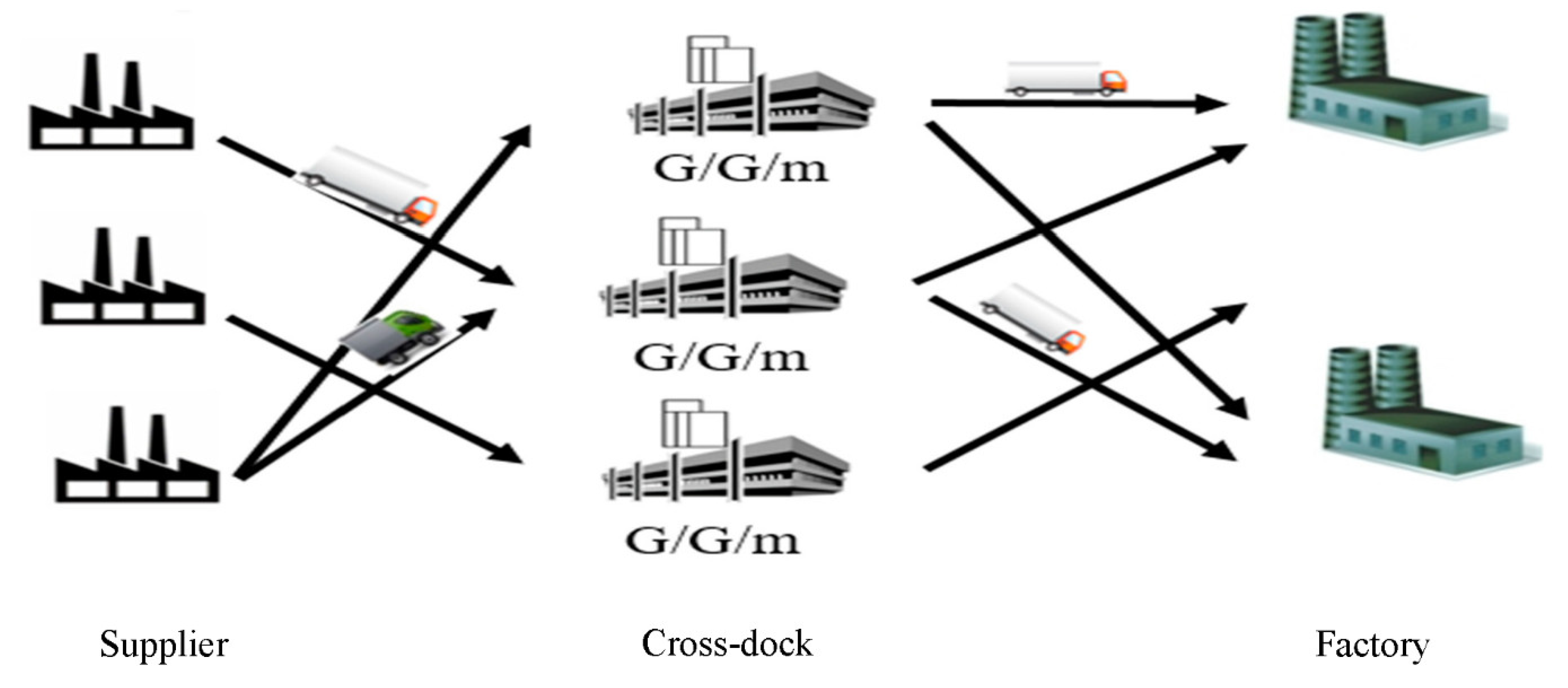
- The second level includes cross-docks or distribution centers.
- Warehouse locations are not determined in advance and are chosen from among several potential locations.
- There are several servers in each warehouse in charge of receiving, packaging, and sending items.
- Warehouses are of cross-dock type and items are sent as soon as they are packaged. Hence, storage costs are neglected.
- Location costs are fixed and unique and determined based on warehouse location.
- The third level includes a factory which is in charge of producing the final product.
- Factory location is not predetermined and the final location is selected from among several potential locations.
- Which potential suppliers should be established so that related costs are minimized?
- Which potential warehouses should be established so that related costs are minimized?
- Which potential factories should be established so that related costs are minimized?
- Allocation decisions
- Which active suppliers should be chosen by warehouses for supplying their desired products so that total cost is minimized?
- Which active warehouses should be chosen by factories for supplying their desired products so that total cost is minimized?
- Which transportation vehicle should be selected for transferring products between suppliers and warehouses?
- Which transportation vehicle should be selected for transferring products between warehouses and factories?
- The discharging process for input vehicles follows first in first out. It means that the first input vehicle that enters the cross-docks area is allocated to a free entrance door if there is any; otherwise, it will wait in the area.
- Door capacities are the same in each warehouse.
- Input and output trucks are not allowed to exit the warehouse and interrupt their respective services until the discharging and loading processes are over.
- Servicing time (load discharging) in each door is probable and follows a general probability distribution.
- Warehouses and factories are capacitated.
- Supplier locations
- Cross-dock locations
- Factory locations
- Allocating suppliers to warehouses
- Allocating warehouses to factories
- Determining item transportation between suppliers and warehouses
- Determining item transportation between warehouses and factories
- Determining the number of existing doors in each warehouse
2.1. Genetic Algorithm
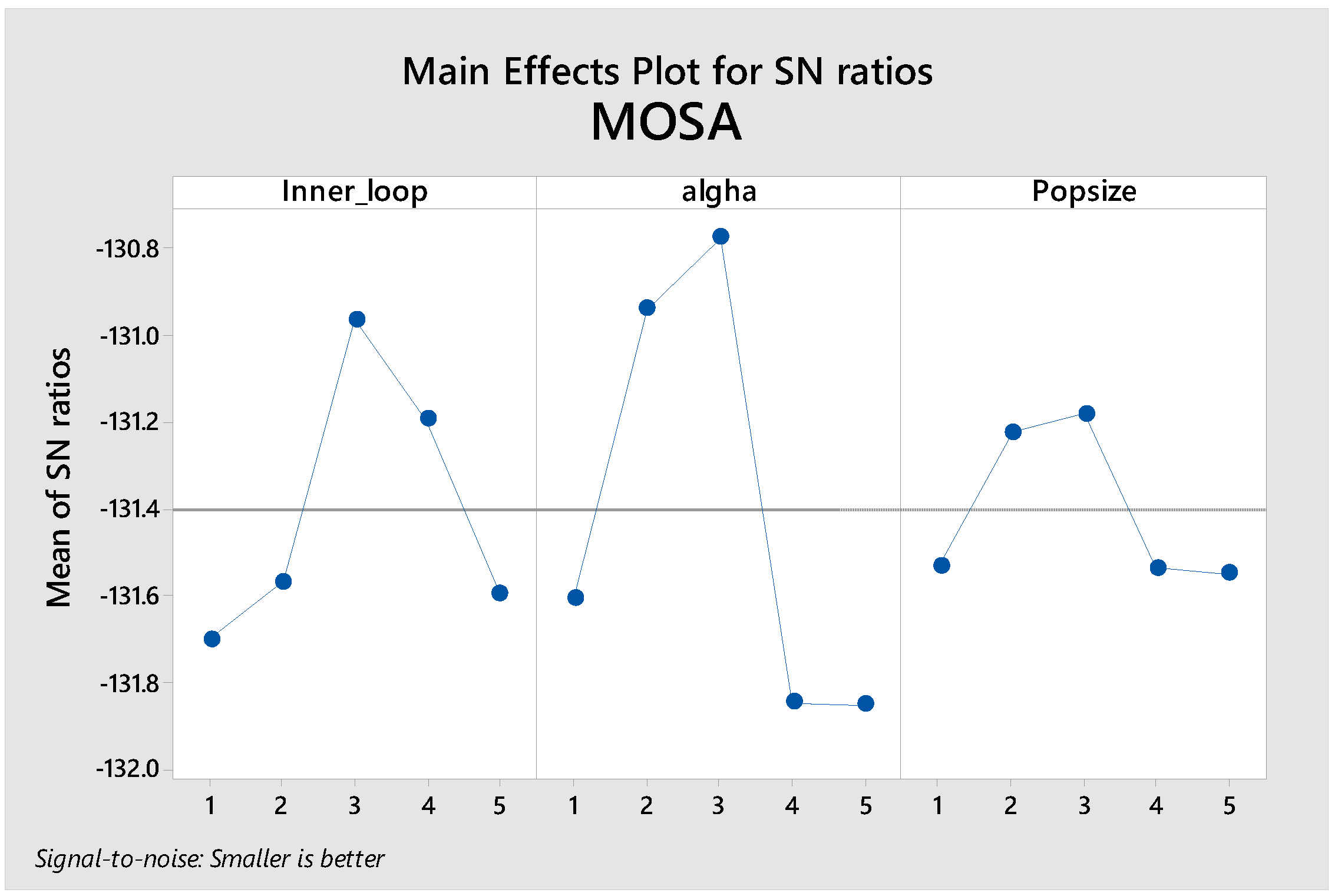
2.2. Multi-Objective Simulated Annealing Algorithm (MOSA)
2.3. Multi-Objective Water Flow Algorithm (MOWFA)
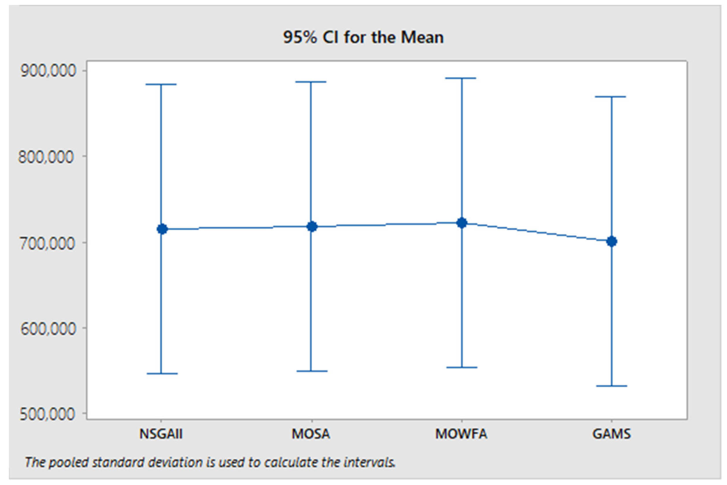
3. Discussion and Results Evaluation
4. Conclusions and Suggestions for Future Work
Author Contributions
Funding
Institutional Review Board Statement
Informed Consent Statement
Data Availability Statement
Conflicts of Interest
Ethical Approval
References
- Agustina, D.; Lee, C.; Piplani, R. A Review: Mathematical Modles for Cross Docking Planning. Int. J. Eng. Bus. Manag. 2010, 2, 47–54. [Google Scholar] [CrossRef]
- Van Belle, J.; Valckenaers, P.; Cattrysse, D. Cross-docking: State of the art. J. Omega 2012, 40, 827–846. [Google Scholar] [CrossRef]
- Apte, U.M.; Viswanathan, S. Effective Cross Docking for Improving Distribution Efficiencies. Int. J. Logist. Res. Appl. 2000, 3, 291–302. [Google Scholar] [CrossRef]
- Bachlaus, M.; Pandey, M.K.; Mahajan, C.; Shankar, R.; Tiwari, M.K. Designing an integrated multi-echelon agile supply chain network: A hybrid taguchi-particle swarm optimization approach. J. Intell. Manuf. 2008, 19, 747–761. [Google Scholar] [CrossRef]
- Yu, W. Operational Strategies for Cross Docking Systems. Ph.D. Thesis, Iowa State University, Ames, IA, USA, 2002. [Google Scholar]
- Magableh, G.; Rossetti, M.; Mason, S. Modeling and Analysis of a Generic Cross-Docking Facility. In Proceedings of the 37th Winter Simulation Conference, Orlando, FL, USA, 4 December 2005; pp. 1613–1620. [Google Scholar] [CrossRef]
- Ley, S.; Elfayoumy, S. Cross Dock Scheduling Using Genetic Algorithms. In Proceedings of the 2007 International Symposium on Computational Intelligence in Robotics and Automation, Jacksonville, FL, USA, 20–23 June 2007; pp. 416–420. [Google Scholar] [CrossRef]
- Yu, W.; Egbelu, P.J. Scheduling of inbound and outbound trucks in cross docking systems with temporary storage. Eur. J. Oper. Res. 2008, 184, 377–396. [Google Scholar] [CrossRef]
- Chen, F.; Lee, C.-Y. Minimizing the makespan in a two-machine cross-docking flow shop problem. Eur. J. Oper. Res. 2009, 193, 59–72. [Google Scholar] [CrossRef]
- Vahdani, B.; Zandieh, M. Scheduling trucks in cross-docking systems: Robust meta-heuristics. Comput. Ind. Eng. 2010, 58, 12–24. [Google Scholar] [CrossRef]
- Dondo, R.; Cerdá, J. The heterogeneous vehicle routing and truck scheduling problem in a multi-door cross-dock system. Comput. Chem. Eng. 2015, 76, 42–62. [Google Scholar] [CrossRef]
- Moghadam, S.S.; Ghomi, S.F.; Karimi, B. Vehicle routing scheduling problem with cross docking and split deliveries. Comput. Chem. Eng. 2014, 69, 98–107. [Google Scholar] [CrossRef]
- Ahmadizar, F.; Zeynivand, M.; Arkat, J. Two-level vehicle routing with cross-docking in a three-echelon supply chain: A genetic algorithm approach. Appl. Math. Model. 2015, 39, 7065–7081. [Google Scholar] [CrossRef]
- Yu, V.F.; Jewpanya, P.; Redi, A.A.N.P. Open vehicle routing problem with cross-docking. Comput. Ind. Eng. 2016, 94, 6–17. [Google Scholar] [CrossRef]
- Amini, A.; Tavakkoli-Moghaddam, R. A bi-objective truck scheduling problem in a cross-docking center with probability of breakdown for trucks. Comput. Ind. Eng. 2016, 96, 180–191. [Google Scholar] [CrossRef]
- Cóccola, M.; Mendez, C.; Dondo, R.G. A branch-and-price approach to evaluate the role of cross-docking operations in consolidated supply chains. Comput. Chem. Eng. 2015, 80, 15–29. [Google Scholar] [CrossRef]
- Utama, D.N.; Zaki, F.A.; Munjeri, I.J.; Putri, N.U. A water flow algorithm based optimization model for road traffic engineering. In Proceedings of the International Conference on Advanced Computer Science and Information Systems (ICACSIS), Malang, Indonesia, 15–16 October 2016; pp. 591–596. [Google Scholar] [CrossRef]
- Hasani Goodarzi, A.; Nahavandi, N.; Zegordi, S.H. A Multi-Objective Imperialist Competitive Algorithm for Vehicle Routing Problem in Cross-docking Networks with Time Windows. J. Ind. Syst. Eng. 2018, 11, 1–23. [Google Scholar]
- Ahkamiraad, A.; Wang, Y. Capacitated and multiple cross-docked vehicle routing problem with pickup, delivery, and time windows. Comput. Ind. Eng. 2018, 119, 76–84. [Google Scholar] [CrossRef]
- Baniamerian, A.; Bashiri, M.; Zabihi, F. Two phase genetic algorithm for vehicle routing and scheduling problem with cross-docking and time windows considering customer satisfaction. J. Ind. Eng. Int. 2018, 14, 15–30. [Google Scholar] [CrossRef]
- Molavi, D.; Shahmardan, A.; Sajadieh, M.S. Truck scheduling in a cross docking systems with fixed due dates and shipment sorting. Comput. Ind. Eng. 2018, 117, 29–40. [Google Scholar] [CrossRef]
- Fonseca, G.B.; Nogueira, T.H.; Ravetti, M.G. A hybrid Lagrangian metaheuristic for the cross-docking flow shop scheduling problem. Eur. J. Oper. Res. 2018, 275, 139–154. [Google Scholar] [CrossRef]
- Gelareh, S.; Glover, F.; Guemri, O.; Hanafi, S.; Nduwayo, P.; Todosijević, R. A comparative study of formulations for a cross-dock door assignment problem. Omega 2018, 91, 102015. [Google Scholar] [CrossRef]
- Musavi, M.M.; Tavakkoli-Moghaddam, R.; Rayat, F. A bi-objective model for pickup and delivery pollution routing problem with integration and consolidation shipments in cross-docking system. Iran. J. Oper. Res. 2018, 8, 2–14. [Google Scholar] [CrossRef][Green Version]
- Nassief, W.; Contreras, I.; Jaumard, B. A comparison of formulations and relaxations for cross-dock door assignment problems. Comput. Oper. Res. 2018, 94, 76–88. [Google Scholar] [CrossRef]
- Shaelaie, M.-H.; Ranjbar, M.; Jamili, N. Integration of parts transportation without cross docking in a supply chain. Comput. Ind. Eng. 2018, 118, 67–79. [Google Scholar] [CrossRef]
- Baniamerian, A.; Bashiri, M.; Tavakkoli-Moghaddam, R. Modified variable neighborhood search and genetic algorithm for profitable heterogeneous vehicle routing problem with cross-docking. Appl. Soft Comput. 2019, 75, 441–460. [Google Scholar] [CrossRef]
- Seyedi, I.; Hamedi, M.; Tavakkoli-Moghaddam, R. Truck Scheduling in a Cross-Docking Terminal by Using Novel Robust Heuristics. Int. J. Eng. 2019, 32, 296–305. [Google Scholar]
- Rijal, A.; Bijvank, M.; de Koster, R. Integrated scheduling and assignment of trucks at unit-load cross-dock terminals with mixed service mode dock doors. Eur. J. Oper. Res. 2019, 278, 752–771. [Google Scholar] [CrossRef]
- Corsten, H.; Becker, F.; Salewski, H. Integrating truck and workforce scheduling in a cross-dock: Analysis of different workforce coordination policies. J. Bus. Econ. 2019, 90, 207–237. [Google Scholar] [CrossRef]
- Dulebenets, M.A. A Delayed Start Parallel Evolutionary Algorithm for just-in-time truck scheduling at a cross-docking facility. Int. J. Prod. Econ. 2019, 212, 236–258. [Google Scholar] [CrossRef]
- Rahbari, A.; Nasiri, M.M.; Werner, F.; Musavi, M.; Jolai, F. The vehicle routing and scheduling problem with cross-docking for perishable products under uncertainty: Two robust bi-objective models. Appl. Math. Model. 2019, 70, 605–625. [Google Scholar] [CrossRef]
- Hadipour, H.; Amiri, M.; Sharifi, M. Redundancy allocation in series-parallel systems under warm standby and active components in repairable subsystems. Reliab. Eng. Syst. Saf. 2019, 192, 106048. [Google Scholar] [CrossRef]
- Khorshidian, H.; Shirazi, M.A.; Ghomi, S.M.T.F. An intelligent truck scheduling and transportation planning optimization model for product portfolio in a cross-dock. J. Intell. Manuf. 2019, 30, 163–184. [Google Scholar] [CrossRef]
- Fard, S.S.; Vahdani, B. Assignment and scheduling trucks in cross-docking system with energy consumption consideration and trucks queuing. J. Clean. Prod. 2019, 213, 21–41. [Google Scholar] [CrossRef]
- Goodarzi, A.H.; Tavakkoli-Moghaddam, R.; Amini, A. A new bi-objective vehicle routing-scheduling problem with cross-docking: Mathematical model and algorithms. Comput. Ind. Eng. 2020, 149, 106832. [Google Scholar] [CrossRef]
- Movassaghi, M.; Avakh Darestani, S. Cross-docks scheduling with multiple doors using fuzzy approach. Eur. Transp. 2020, 79, 2. [Google Scholar] [CrossRef]
- Goodarzi, A.H.; Zegordi, S.H. Vehicle routing problem in a kanban controlled supply chain system considering cross-docking strategy. Oper. Res. 2020, 20, 2397–2425. [Google Scholar] [CrossRef]
- Ardakani, A.; Fei, J.; Beldar, P. Truck-to-door sequencing in multi-door cross-docking system with dock repeat truck holding patter. Int. J. Ind. Eng. Comput. 2020, 11, 201–220. [Google Scholar] [CrossRef]
- Nogueira, T.H.; Coutinho, F.P.; Ribeiro, R.P.; Ravetti, M.G. Parallel-machine scheduling methodology for a multi-dock truck sequencing problem in a cross-docking center. Comput. Ind. Eng. 2020, 143, 106391. [Google Scholar] [CrossRef]
- Nikzamir, M.; Baradaran, V. A healthcare logistic network considering stochastic emission of contamination: Bi-objective model and solution algorithm. Transp. Res. Part E Logist. Transp. Rev. 2020, 142, 102060. [Google Scholar] [CrossRef] [PubMed]
- Shahabi-Shahmiri, R.; Asian, S.; Tavakkoli-Moghaddam, R.; Mousavi, S.M.; Rajabzadeh, M. A routing and scheduling problem for cross-docking networks with perishable products, heterogeneous vehicles and split delivery. Comput. Ind. Eng. 2021, 157, 107299. [Google Scholar] [CrossRef]
- Castellucci, P.B.; Costa, A.M.; Toledo, F. Network scheduling problem with cross-docking and loading constraints. Comput. Oper. Res. 2021, 132, 105271. [Google Scholar] [CrossRef]
- Goodarzi, A.H.; Diabat, E.; Jabbarzadeh, A.; Paquet, M. An M/M/c queue model for vehicle routing problem in multi-door cross-docking environments. Comput. Oper. Res. 2021, 138, 105513. [Google Scholar] [CrossRef]
- Goodarzi, A.H.; Zegordi, S.H.; Alpan, G.; Kamalabadi, I.N.; Kashan, A.H. Reliable cross-docking location problem under the risk of disruptions. Oper. Res. 2021, 21, 1569–1612. [Google Scholar] [CrossRef]
- Yu, V.F.; Jewpanya, P.; Redi, A.P.; Tsao, Y.-C. Adaptive neighborhood simulated annealing for the heterogeneous fleet vehicle routing problem with multiple cross-docks. Comput. Oper. Res. 2021, 129, 105205. [Google Scholar] [CrossRef]
- Theophilus, O.; Dulebenets, M.A.; Pasha, J.; Lau, Y.-Y.; Fathollahi-Fard, A.M.; Mazaheri, A. Truck scheduling optimization at a cold-chain cross-docking terminal with product perishability considerations. Comput. Ind. Eng. 2021, 156, 107240. [Google Scholar] [CrossRef]
- Qiu, Y.; Zhou, D.; Du, Y.; Liu, J.; Pardalos, P.M.; Qiao, J. The two-echelon production routing problem with cross-docking satellites. Transp. Res. Part E Logist. Transp. Rev. 2021, 147, 102210. [Google Scholar] [CrossRef]
- Smith, A.; Toth, P.; Bam, L.; van Vuuren, J. A multi-tiered vehicle routing problem with global cross-docking. Comput. Oper. Res. 2022, 137, 105526. [Google Scholar] [CrossRef]


| Authors | Year | Objectives | Objective Function | Metaheuristic Method | Exact Solution, Software | Multi-Suppliers | Multi-Products | Time Window | Case Study |
|---|---|---|---|---|---|---|---|---|---|
| Ahmadizar et al. | 2015 [14] | Cost | Multi- | Hybrid genetic algorithm | CPLEX | ✓ | ✓ | - | - |
| Cóccola et al. | 2015 [16] | Cost | Single | Branch-and-price algorithm | CPLEX | ✓ | ✓ | ✓ | ✓ |
| Utama et al. | 2016 [17] | Road traffic flow | Single | Water flow algorithm (WFA) | CPLEX | ✓ | ✓ | - | ✓ |
| Hasani Goodarzi et al. | 2018 [18] | Time, Cost | Multi- | Multi-objective imperialist competitive algorithm (MOICA) | MATLAB | ✓ | ✓ | ✓ | - |
| Ahkamiraad and Wang | 2018 [19] | Cost | Multi- | Hybrid of the genetic algorithm and particle swarm optimization (HGP) | CPLEX | ✓ | ✓ | ✓ | - |
| Baniamerian et al. | 2018 [20] | Cost | Multi- | Genetic algorithm (GA) | CPLEX/MATLAB | ✓ | ✓ | ✓ | - |
| Molavi et al. | 2018 [21] | Cost | Multi- | Hybrid genetic algorithm-reduced variable neighborhood search algorithm (HGARVNS) | GAMS/MATLAB | ✓ | ✓ | ✓ | - |
| Fonseca et al. | 2018 [22] | Time | Single | Hybrid Lagrangian Metaheuristic | CPLEX | ✓ | ✓ | - | - |
| Gelareh et al. | 2018 [23] | Cost | Single | - | CPLEX | ✓ | ✓ | - | - |
| Musavi et al. | 2018 [24] | Time, Fuel consumption | Multi- | Archived multi-objective simulated annealing (AMOSA) | MATLAB | ✓ | ✓ | ✓ | - |
| Nassief et al. | 2018 [25] | Cost | Multi- | Column generation algorithm | CPLEX | ✓ | ✓ | - | - |
| Shaelaie et al. | 2018 [26] | Cost | Multi- | Rounding algorithm (RA), Single-period algorithm (SPA) | CPLEX | ✓ | ✓ | - | - |
| Baniamerian et al. | 2019 [27] | Cost | Multi- | Novel genetic algorithm hybridized with modified VNS (GA-MVNS), Artificial bee colony (ABC) algorithm, Simulated annealing (SA) | GAMS | ✓ | ✓ | ✓ | - |
| Seyedi et al. | 2019 [28] | Time | Single | Cross-Dock Heuristic | GAMS | ✓ | ✓ | ✓ | - |
| Rijal et al. | 2019 [29] | Cost | Multi- | Adaptive large neighbourhood search (ALNS) | Python, Gurobi Optimizer | ✓ | ✓ | ✓ | ✓ |
| Corsten et al. | 2019 [30] | Cost | Single | - | Gurobi Optimizer | ✓ | ✓ | ✓ | ✓ |
| Dulebenets | 2019 [31] | Cost | Multi- | Novel delayed start parallel evolutionary algorithm | GAMS/CPLEX | ✓ | ✓ | - | - |
| Rahbari et al. | 2019 [32] | Cost, Weight | Multi- | - | GAMS/CPLEX | ✓ | ✓ | ✓ | - |
| Hadipour et al. | 2019 [33] | Cost | Multi- | Multi-objective water-flow algorithm (MOWFA) | MATLAB | ✓ | ✓ | - | - |
| Khorshidian et al. | 2019 [34] | Time, Cost | Multi- | - | LINGO | ✓ | ✓ | ✓ | ✓ |
| Fard and Vahdani | 2019 [35] | Cost, Energy | Multi- | Multi-objective imperialist competitive algorithm (MOICA), Multi-objective grey wolf optimizer (MOGWO) | GAMS | ✓ | ✓ | ✓ | - |
| Hasani Goodarzi et al. | 2020 [36] | Time, Cost | Multi- | Multi-objective evolutionary algorithm (MOEA) | GAMS | ✓ | ✓ | ✓ | ✓ |
| Movassaghi and Avakh Darestani | 2020 [37] | Time, Cost | Multi- | - | GAMS | ✓ | ✓ | ✓ | - |
| Hasani Goodarzi and Zegordi | 2020 [38] | Cost | Multi- | Memetic algorithm | GAMS/CPLEX | ✓ | ✓ | - | - |
| Ardakani et al. | 2020 [39] | Time | Single | Heuristic algorithm | GAMS | ✓ | ✓ | ✓ | - |
| Nogueira et al. | 2020 [40] | Time | Single | Constructive heuristic | CPLEX | ✓ | ✓ | ✓ | - |
| Nikzamir and Baradaran | 2020 [41] | Cost, Emission of contamination | Multi- | Multi-objective water flow algorithm (MOWFA) | MATLAB | ✓ | ✓ | ✓ | ✓ |
| Shahabi-Shahmiri et al. | 2021 [42] | Time, Cost, Capacity utilization rate | Multi- | - | GAMS | ✓ | ✓ | ✓ | ✓ |
| Castellucci et al. | 2021 [43] | Cost | Multi- | - | GAMS | ✓ | ✓ | ✓ | - |
| Hasani Goodarzi et al. | 2021 [44] | Cost | Multi- | Lagrangian relaxation algorithms | GAMS/CPLEX | ✓ | ✓ | - | ✓ |
| Hasani Goodarzi et al. | 2021 [45] | Cost | Multi- | Genetic algorithm (GA) | GAMS | ✓ | - | - | ✓ |
| Yu et al. | 2021 [46] | Cost | Multi- | Adaptive neighborhood simulated annealing algorithm | C# | ✓ | ✓ | - | - |
| Theophilus et al. | 2021 [47] | Cost | Multi- | Evolutionary algorithm | GAMS | ✓ | ✓ | ✓ | - |
| Qiu et al. | 2021 [48] | Cost | Multi- | Branch-and-cut algorithm | CPLEX | ✓ | ✓ | - | - |
| Smith et al. | 2022 [49] | Time, Vehicles | Multi- | Multi-objective ant colony optimization (MACO) algorithm | CPLEX | ✓ | ✓ | - | ✓ |
| Indices | Description |
|---|---|
| I | Suppliers index |
| J | Cross-dock index |
| K | Factory index |
| V | Vehicle index |
| Parameters | Description |
| Maximum number of allowed suppliers | |
| Maximum number of allowed cross-docks | |
| Maximum number of allowed factories | |
| Demand entrance rate from supplier i | |
| Service rate for each sever in cross-dock j | |
| Fixed cost of locating supplier in potential node i | |
| Fixed cost of locating supplier in potential node j | |
| Fixed cost of locating factory in potential node k | |
| Shipping cost from supplier i to cross-dock j via vehicle v | |
| Shipping cost from cross-dock j to factory k via vehicle v | |
| Shipping time from supplier i to cross-dock j via vehicle v | |
| Shipping time from cross-dock j to factory k via vehicle v | |
| Employing cost for each server in cross-dock j | |
| Maximum number of servers who can be placed in cross-dock j |
| Number of existing servers in cross-dock j |
| Supplier | 5 | 5 | 6 |
| Vehicle | 4 | 2 | 6 |
| Cross-dock | 3 | 3 | 6 |
| Transportation Vehicle | 8 | 4 | 1 |
| Factory | 4 | 4 | 3 |
| Algorithm | Parameters | Description | First Level | Second Level | Third Level | Fourth Level | Fifth Level |
|---|---|---|---|---|---|---|---|
| MOWFA | Pop size | The number of first flows | 10 | 20 | 30 | 40 | 50 |
| M0 | The initial mass | 50 | 60 | 70 | 80 | 90 | |
| V0 | The initial speed | 20 | 30 | 40 | 50 | 60 | |
| MOSA | Inner loop | The number of iterations in the inner loop | 10 | 20 | 30 | 40 | 50 |
| alpha | Temperature reduction rate | 0.95 | 0.96 | 0.97 | 0.98 | 0.99 | |
| Pop size | Population size | 10 | 15 | 20 | 30 | 40 | |
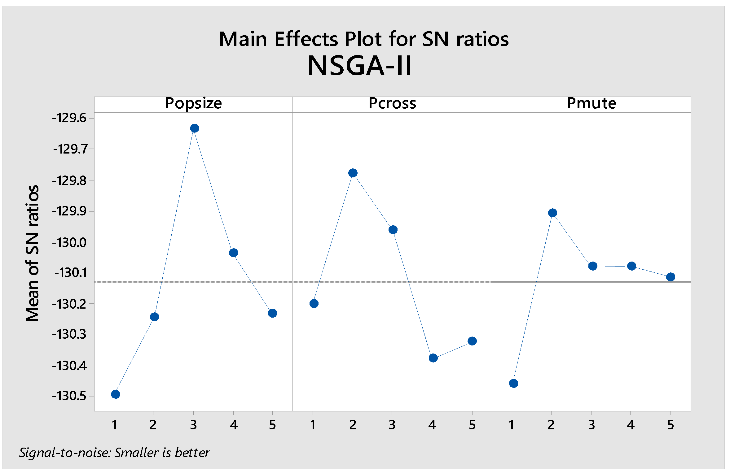
| NSGA-II | Pop size | The initial population size | 60 | 80 | 100 | 120 | 140 |
| Pc | Crossover rate | 0.75 | 0.80 | 0.85 | 0.90 | 0.95 | |
| Pm | Mutation rate | 0.05 | 0.07 | 0.09 | 0.12 | 0.15 |
Publisher’s Note: MDPI stays neutral with regard to jurisdictional claims in published maps and institutional affiliations. |
© 2022 by the authors. Licensee MDPI, Basel, Switzerland. This article is an open access article distributed under the terms and conditions of the Creative Commons Attribution (CC BY) license (https://creativecommons.org/licenses/by/4.0/).
Share and Cite
Rostami, P.; Avakh Darestani, S.; Movassaghi, M. Modelling Cross-Docking in a Three-Level Supply Chain with Stochastic Service and Queuing System: MOWFA Algorithm. Algorithms 2022, 15, 265. https://doi.org/10.3390/a15080265
Rostami P, Avakh Darestani S, Movassaghi M. Modelling Cross-Docking in a Three-Level Supply Chain with Stochastic Service and Queuing System: MOWFA Algorithm. Algorithms. 2022; 15(8):265. https://doi.org/10.3390/a15080265
Chicago/Turabian StyleRostami, Parinaz, Soroush Avakh Darestani, and Mitra Movassaghi. 2022. "Modelling Cross-Docking in a Three-Level Supply Chain with Stochastic Service and Queuing System: MOWFA Algorithm" Algorithms 15, no. 8: 265. https://doi.org/10.3390/a15080265
APA StyleRostami, P., Avakh Darestani, S., & Movassaghi, M. (2022). Modelling Cross-Docking in a Three-Level Supply Chain with Stochastic Service and Queuing System: MOWFA Algorithm. Algorithms, 15(8), 265. https://doi.org/10.3390/a15080265