Similar Supergraph Search Based on Graph Edit Distance

Abstract

Subgraph and supergraph search methods are promising techniques for the development of new drugs. For example, the chemical structure of favipiravir—an antiviral treatment for influenza—resembles the structure of some components of RNA. Represented as graphs, such compounds are similar to a subgraph of favipiravir. However, the existing supergraph search methods can only discover compounds that match exactly. We propose a novel problem, called similar supergraph search, and design an efficient algorithm to solve it. The problem is to identify all graphs in a database that are similar to any subgraph of a query graph, where similarity is defined as edit distance. Our algorithm represents the set of candidate subgraphs by a code tree, which it uses to efficiently compute edit distance. With a distance threshold of zero, our algorithm is equivalent to an existing efficient algorithm for exact supergraph search. Our experiments show that the computation time increased exponentially as the distance threshold increased, but increased sublinearly with the number of graphs in the database.

1. Introduction

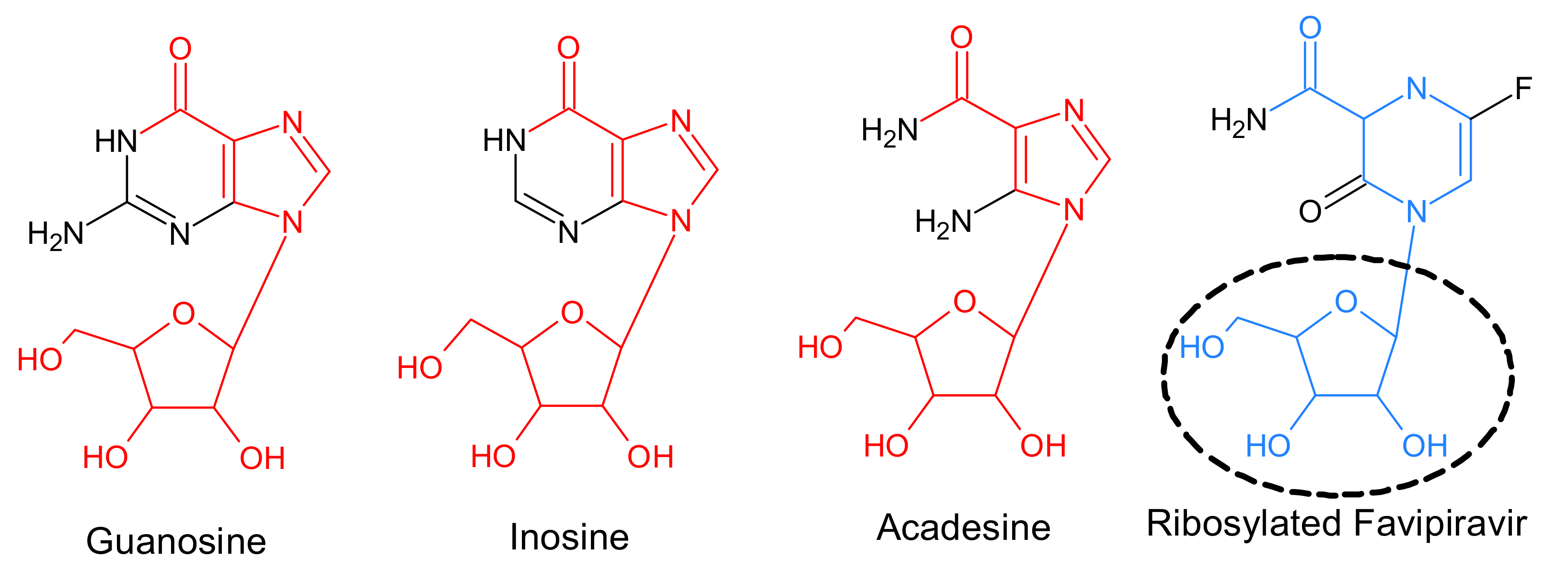
The coronavirus disease (COVID-19) has been spreading widely since 2019. In Japan, favipiravir (brand name: Avigan) has been examined as a promising antiviral medication against COVID-19. Favipiravir was initially developed as a medication to treat influenza. When Favipiravir is ribosylated, its structure resembles acadesine, which is a precursor to inosine. Inosine is the previous stage of guanosine and adenosine, which are components of RNA [1]. With this treatment, the RNA synthetase of a virus mistakenly incorporates favipiravir, instead of guanosine, into the replicating virus. This causes RNA synthesis to stop and limits the replication of viruses inside the body.

Figure 1 shows the chemical structures of guanosine, inosine, acadesine, and ribosylated favipiravir. The substructure $\alpha$, drawn in red, is common to all of guanosine, inosine, and acadesine. Therefore, in order to find candidate compounds for a new drug, it may be useful to search for compounds containing a substructure, provided as a query, in a database that consist of many compounds (i.e., substructure search). Conversely, if many substructures relevant to new drug development are known, it can be useful to search for substructures contained in a newly developed chemical compound, provided as a query, in a database recording these substructures (i.e., superstructure search). This paper discusses methods related to the latter task. The substructure drawn in blue in Figure 1 is similar to the substructure $\alpha$, but they do not match perfectly. In the situation shown, the substructure $\alpha$, which contributes to anti-influenza agents, is registered in a database. The database contains various substructures for which its medicinal effects, side effects and so on are known. If ribosylated favipiravir is given as the query and the substructure $\alpha$ is the output as the search result, we may be able to discover that ribosylated favipiravir is anti-influenza. Therefore, such a search engine for chemical compounds would be very useful and effective.

Figure 1. Similar Chemical Compounds.

A compound can be represented as a graph, in which the vertices and edges correspond to the atoms and chemical bonds, respectively. The aforementioned substructure and superstructure search correspond to subgraph search [2,3,4,5,6,7,8,9,10,11,12,13,14] and supergraph search [15,16,17,18,19,20,21,22], respectively, which are actively being studied by researchers. A graph is a highly versatile data structure for representing information in many fields. It can be used to represent human relationship networks, protein interaction networks, resource description frameworks (RDF), computer-aided designs (CAD), and computer vision images; moreover, subgraph and supergraph search are used for many applications in addition to searching for compounds. However, there is no method for searching for graphs that are similar to subgraphs of a query graph and no method applicable to the resemblance between substructures shown in Figure 1. This paper proposes the problem of similar supergraph search and also proposes a method to solve it.

In this paper, we measure the similarity between two graphs g and $g^{\prime }$ by the graph edit distance. The graph edit distance is the minimum number of edits required to transform g to another $g^{\prime }$, where an edit is either an insertion, deletion, or relabeling of a vertex or edge. The number of graphs obtained by editing the graph g$\theta$ times increases drastically, especially when the numbers of vertices and edges are large and the varieties of vertex and edge labels are wide. Such a drastic increase in edited graphs makes it difficult to find similar graphs. However, some real applications need to obtain a subset of graphs edited $\theta$ times. For example, editing the substructure in a broken ellipse of Figure 1 is not admissible, whereas editing the remainder of the blue substructure is admissible. By restricting an editable part in the structure, the number of graphs obtained by editing the graph g$\theta$ times is decreased. In our proposed method, users can search for their desired type of similar graphs in a database containing graphs and this search can be realized by simply rewriting only one function without the need to modify our proposed algorithm. Therefore, the method proposed in this paper is a general and flexible framework for searching for similar subgraphs of query graphs and is easily customizable for searching for the types of graphs desired by the user.

The remainder of the paper is organized as follows. Section 2 formalizes the novel problem of searching for graphs contained in a query graph in a database storing many graphs and Section 3 discusses related work. In Section 4 and Section 5, we propose straightforward methods for a simpler problem in which the searched graphs are constrained. In Section 6 and Section 7, we propose a novel method for solving the original problem by extending the above methods. In Section 8, we analyze the computational efficiency of the proposed method by using real-world datasets. Finally, we conclude the paper in Section 9.

2. Problem Definition

A labeled graph is expressed as $g=(V,E,\mathsf{\Sigma },\ell )$, where V is a set of vertices, $E\subseteq V\times V$ is a set of edges, $\mathsf{\Sigma }$ is a set of labels for the vertices and edges, and $\ell :V\cup E\to \mathsf{\Sigma }$ is a function to assign the labels to the vertices and edges. We denote the set of all vertices in graph g as $V\left(g\right)$. A graph g is called a directed graph if the edges in g have directions; otherwise, g is called an undirected graph. A sequence of edges from $v_1$ to $v_2$ is called a path and a graph (for a directed graph, all edges in the graph are replaced with undirected edges.) and a path that exists between any two vertices is called connected.

Given graphs $g=(V,E,\mathsf{\Sigma },\ell )$ and $g^{\prime }=(V^{\prime },E^{\prime },{\mathsf{\Sigma }}^{\prime },{\ell }^{\prime })$, $\forall v,v_1,v_2\in V^{\prime }$, when an injective function $\varphi :V^{\prime }\to V$ fulfills the following conditions, $g^{\prime }$ is called a subgraph of g, which is denoted as $g^{\prime }\subseteq g$:

• $(\varphi \left(v_1\right),\varphi \left(v_2\right))\in E$ if $(v_1,v_2)\in E^{\prime }$;
• ${\ell }^{\prime }\left(v\right)=\ell \left(\varphi \left(v\right)\right)$;
• ${\ell }^{\prime }\left((v_1,v_2)\right)=\ell \left((\varphi \left(v_1\right),\varphi \left(v_2\right))\right)$.

In addition, when $(\varphi \left(v_1\right),\varphi \left(v_2\right))\in E$ iff $(v_1,v_2)\in E^{\prime }$, we call $g^{\prime }$ an induced subgraph of g, which is denoted as $g^{\prime }{\subseteq }_{i}g$. Although this paper focuses only on undirected and connected graphs, the methods proposed can easily be extended to directed or unconnected graphs.

The graph edit distance is the minimum number of edits required to transform a graph g to another graph $g^{\prime }$, where an edit is either an insertion, deletion, or relabeling of a vertex or edge. In this paper, we assume that the cost of each edit is 1. The number of edits between graphs $g=(V,E,\mathsf{\Sigma },\ell )$ and $g^{\prime }=(V^{\prime },E^{\prime },\mathsf{\Sigma },{\ell }^{\prime })$ is defined as follows:

$$dist(g,g^{\prime },\phi )=\sum _{i=1}^{|V^{\prime }|}{c}_{i\phi \left(i\right)}+\sum _{i=1}^{|V^{\prime }|-1}\sum _{j=i+1}^{|V^{\prime }|}c\left((v_i,v_j)\to \left(v_{\phi \left(i\right)},v_{\phi \left(j\right)}\right)\right),$$

(1)

where we assume that $\left|V\right|\le |V^{\prime }|$ and V is extended to $V^{+}=V\cup \{{\epsilon }_1,{\epsilon }_2,\dots ,{\epsilon }_{|V^{\prime }|-|V|}\}$ [23]. In addition, when g is transformed to $g^{\prime }$, the mapping between V and $V^{\prime }$ is expressed as a bijective mapping $\phi :V^{+}\to V^{\prime }$. $c_{ij}$ is the cost to edit the vertex $v_i\in V^{+}$ to $v_j\in V^{\prime }$ and $c((v_i,v_j)\to (v_{i^{\prime }},v_{j^{\prime }}))$ is the cost to edit edge $(v_i,v_j)\in E$ to $(v_{i^{\prime }},v_{j^{\prime }})\in E^{\prime }$. Editing ${\epsilon }_i\in V^{+}$ to $v_j\in V^{\prime }$ means performing a vertex insertion in $g^{\prime }$. Therefore, the graph edit distance $ed(g,g^{\prime })$ between the graphs g and $g^{\prime }$ is defined as follows:

$$ed(g,g^{\prime })=\underset{\phi \in \mathsf{\Phi }\left(\right|V^{\prime }|,|V^{\prime }\left|\right)}{min}dist(g,g^{\prime },\phi ),$$

(2)

where $\mathsf{\Phi }(\alpha ,\beta )$ is a set of all possible $\beta$-permutations of the integers $1,2,\dots ,\alpha$. The solution to Equation (2) is one of the quadratic assignment problems, which are known to be NP-complete.

Given a set of graphs $G=\{g_1,g_2,\dots ,g_n\}$, a query graph q, and a threshold $\theta$ as input, the problem tackled in this paper is to output a set of graphs.

$$S=\{g_i\in G\mid \exists q^{\prime }\subseteq qs.t.ed(g_i,q^{\prime })\le \theta \}.$$

(3)

In Equation (3), note that $q^{\prime }$ is a subgraph of q but not an induced subgraph of q. When $\theta$ is 0 in Equation (3), the problem is equivalent to the original supergraph search problem. Therefore, our problem, represented by Equation (3), is an extension of the supergraph search problem.

3. Related Work

In Section 2, we defined the problem tackled in this paper. Recently, much attention has been focused on searching for graphs satisfying some conditions in a database consisting of multiple graphs. Table 1 summarizes graph search problems and the publications that tackle each problem. The subgraph search problem is to find graphs that contain the query graph and can be expressed as follows:

$$\{g_i\in G\mid q\subseteq g_i\},$$

whereas the supergraph search problem is to find graphs that the query graph contains and it can be expressed as follows.

$$\{g_i\in G\mid g_i\subseteq q\}.$$

Table 1. Summary of graph search problems and references.

	Complete Matching	Similar Matching
graph search	$\{g_i\in G\mid q=g_i\}$	$\{g_i\in G\mid ed(g_i,q)\le \theta \}$ [25,26,27,28,29,30,31,32]
supergraph search	$\{g_i\in G\mid g_i\subseteq q\}$ [15,16,17,18,19,20,21,22]	$\{g_i\in G\mid \exists q^{\prime }\subseteq qs.t.ed(g_i,q^{\prime })\le \theta \}$ This paper (novel problem).
subgraph search	$\{g_i\in G\mid q\subseteq g_i\}$ [2,3,4,5,6,7,8,9,10,11,12,13,14]	$\{g_i\in G\mid \exists g\subseteq g_{i}s.t.ed(g,q)\le \theta \}$ There are no papers to our best knowledge.

These problems contain the subgraph isomorphism problem, which is known to be NP-complete. The similar graph search problem is to find graphs that are similar to the query graph, and can be expressed as

$$\{g_i\in G\mid ed(g_i,q)\le \theta \}.$$

This problem contains the graph edit distance problem, which is known to be NP-complete. Various methods have been proposed to solve these problems. The problem tackled in this paper is to find graphs that are similar to subgraphs of the query graph and contains both the subgraph isomorphism problem and graph edit distance problem. This problem is a novel one, to the best of our knowledge. Since the subgraph isomorphism problem and graph edit distance problem are NP-complete, a naive method for solving either of the problems for a given query graph and for each graph in the database would be unrealistic.

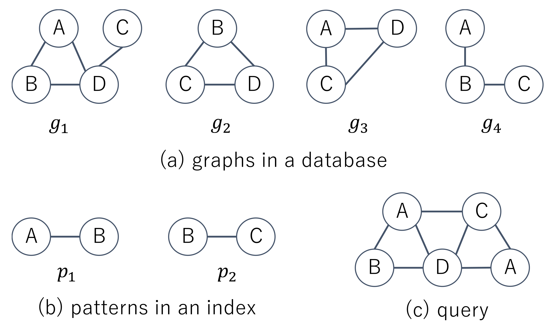
Most of the methods proposed in the articles cited in Table 1 are based on filtering and verification and an index in each of the methods has a set of patterns P extracted from the database in advance. For example, for the supergraph search problem, in the filtering phase,

$$G^{\prime }=G\setminus \bigcup _{p\in P}\{g_i\in G\mid p⊈q,g_i\subseteq q\}$$

is obtained. Subsequently, the verification phase checks whether $g\subseteq q$, for each graph $g\in G^{\prime }$. Figure 2a shows four graphs in a database and two patterns contained in an index. The index has the information that $p_1\subset g_1$, $p_2\subset g_2$, $p_1\subset g_4$, and $p_2\subset g_4$. Given the query shown in Figure 2c, supergraph search methods first check whether $p_1\subseteq q$ and $p_2\subseteq q$ and then obtain $G^{\prime }=\{g_1,g_3\}$ in the filtering phase. In the verification phase, they test whether $g_1\subseteq q$ and $g_3\subseteq q$. Since the number of vertices in $p_2$ is less than one for $g_2$, the computation time to check whether $p_2\subseteq q$ becomes less than one for $g_2\subseteq q$ and we do not need to check whether $g_2\subseteq q$ in the filtering phase. The patterns in P are either paths, trees, cycles, or graphs extracted from databases. The patterns are extracted by the enumeration or mining method. The enumeration method enumerates all subgraphs in graphs in a database, where the subgraphs are restricted to either paths, trees, cycles, or graphs. In contrast, the mining method enumerates all frequent patterns [24], which are defined as

$$F(G,{\sigma }^{\prime })=\{p\mid p\subseteq g_i,g_i\in G,\sigma (p,G)\ge {\sigma }^{\prime }\}$$

from graphs in a database, where $\sigma (p,G)$ is defined as the number of graphs in G containing pattern p:

$$\sigma (p,G)=|\{g_i\in G\mid p\subseteq g_i\}|.$$

Figure 2. Example of supergraph search.

The extracted patterns are stored in a tree or lattice structure in the index of the graph database. Enumerating patterns and mining patterns from a database are time-consuming processes.

CodeTree [17] is a method for the supergraph search problem. It does not distinguish between filtering and verification phases; it filters out graphs that are not contained in a given query graph while verifying unfiltered graphs. In addition, CodeTree does not enumerate or mine patterns in a database. All graphs in a database are stored in the form of one of the graph codes, such as AcGM [33] code or DFS [34] code, in the index in CodeTree. The AcGM and DFS codes are based on adjacency matrices and adjacency lists, which are alternatives to graph representations. The algorithms for constructing an index for a database and searching graphs in the index are independent of the graph codes and, thus, the method can be integrated and extended with various graph codes for representing graphs in accordance with the intended characteristics of those codes. For this reason, the method proposed in this paper is based on CodeTree.

In this paper, we focus on the problems in which each database consists of multiple graphs. Other subgraph search problems are to search for a database which consists of “a single large graph”. Since the number of graphs given as input is two, we need not distinguish the subgraph and supergraph searches. A typical problem of the graph search with a single large graph is to output all embeddings (or occurrences) $\left\{(\varphi \left(v_1\right),\varphi \left(v_2\right),\dots ,\varphi \left(v_{\left|V\right(q\left)\right|}\right))\right\}$ in a large graph g for a query q consisting of vertices $(v_1,v_2,\dots ,v_{\left|V\right(q\left)\right|})$ when the query q is a subgraph of the large graph g. This problem is applicable to RDFs (Resource Description Frameworks), where each subject or object and predicate corresponds to a vertex and edge in a graph, respectively; PPI (Protein-Protein Interaction) networks, where each protein and interaction correspond to a vertex and edge, respectively; and intrusion alert networks where each computer and possible attack such as Denial-of-Service and TCP Service Sweep correspond a vertex and edge, respectively. Some of the methods for solving these kinds of problems use not only exact matching [35,36,37] but also approximate matching [38,39,40,41] with various similarity measures.

The most representative metric for measuring similarity between two graphs is the graph edit distance. Most of methods for graph search problems use this graph edit distance to measure similarities among graphs. Other most representative measures are to use maximum common subgraphs or graph kernels [42,43] between two graphs. There are two types of problems called maximum common induced subgraph problem [44] and maximum common edge subgraph problem [45] and the problems for finding the maximum common subgraphs in two graphs is NP-complete. In contrast, graph kernels have been proposed to classify graphs in the machine learning domain. The random walk graph kernel [46] returns a high similarity of graphs if random walks on the graphs produce similar sequences of vertex and edge labels. The Weisfeiler–Lehman graph kernel [47] uses the Weisfeiler–Lehman test, which was proposed to solve the graph isomorphism problem. The kernel iteratively relabels each vertex v by concatenating a label of v and labels of v’s adjacent vertices and returns high similarity for two relabeled graphs if the graphs have many common labels.

4. Straightforward Method for Constrained Problem

In Section 2, we defined the problem tackled in this paper. Here, for the sake of simplicity, we first provide methods for outputting the following:

$$\{g_i\in G\mid \exists q^{\prime }{\subseteq }_{i}qs.t.ed(g_i,q^{\prime })\le \theta ,q^{\prime }\mathrm{is} \mathrm{connected},|V\left(g_i\right)|\le |V\left(q^{\prime }\right)\left|\right\},$$

(4)

by constraining the original problem. In the subsequent sections, we explain how the method can be extended to solve the original problem.

Definition 1

(AcGM code [33]). Given a graph $g=(V,E,\mathsf{\Sigma },\ell )$, we assign vertex identifiers $u_1,u_2,\dots ,u_{\left|V\right|}$ to vertices in g and assume that a subgraph of g induced by vertices $u_1,u_2,\dots ,u_i(1\le i\le |V\left|\right)$ is connected. g is represented by an adjacency matrix of dimension $\left|V\right|\times \left|V\right|$ for which its elements $x_{i,j}$ are $\ell \left((u_i,u_j)\right)$ if $(u_i,u_j)\in E$ or 0 otherwise. The AcGM code of graph g is defined by concatenating the elements in the upper-right part of the adjacency matrix, as follows:

$$code(g,⟨u_1,u_2,\dots ,u_{\left|V\right|}⟩)=s_1{s}_2\cdots s_{\left|V\right|},$$

(5)

where each code fragment $s_i$ is defined as follows:

$$s_i=\ell \left(u_i\right)x_{1,i}{x}_{2,i}\cdots x_{i-2,i}{x}_{i-1,i}.$$

$s_1{s}_2\cdots s_i$ is called a prefix of Equation (5). In addition, $c_2\subseteq c_1$ means that a prefix of an AcGM code $c_1$ is equal to another AcGM code $c_2$ and a graph expressed by AcGM code c is denoted as $g\left(c\right)$.

Definition 2

(Linear ordering between AcGM codes). When two AcGM codes $\alpha =a_1{a}_2\cdots a_k$ and $\beta =b_1{b}_2\cdots b_h$ fulfill either of the following conditions, we say that $\beta ⪯\alpha$:

• $\exists ts.t.1\le t\le min(k,h)$, $a_q=b_q$ for $q<t$ and $b_t{\prec }_e{a}_t$;
• $\beta \subseteq \alpha$;

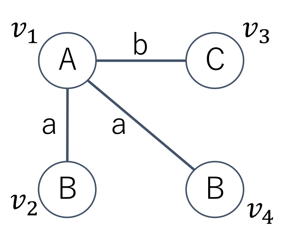
where ${\prec }_e$ is a linear ordering between code fragments [34].

Example 1.

Given the graph with four vertices shown in Figure 3, we have $4!=24$ possible permutations of the four vertices. Among the permutations, according to Definition 1, $code(g,⟨v_2,v_3,v_4,v_1⟩)$ does not generate an AcGM code because a subgraph induced by $⟨v_2,v_3⟩$ is not connected. We can generate 12 AcGM codes from the graph and we show three AcGM codes as follows. Symbols on the left side of the following adjacent matrices are vertex IDs and the letters on the upper side of the matrices are vertex labels. In addition, letters in the matrices are edge labels and zeros in the matrices and they indicate that there are no edges.

Figure 3. Example of a graph.

By concatenating the letters and zeros on sides of arrows in the matrices, three AcGM codes are generated as follows.

$$\begin{array}{ccc}\hfill \alpha & =& code(g,⟨v_1,v_2,v_3,v_4⟩)=ABaCb0Ba00,\hfill \\ \hfill \beta & =& code(g,⟨v_2,v_1,v_3,v_4⟩)=BAaC0bB0a0,and\hfill \\ \hfill \gamma & =& code(g,⟨v_4,v_1,v_2,v_3⟩)=BAaB0aC0b0.\hfill \end{array}$$

The order between the codes is $\alpha \prec \gamma \prec \beta$.

Lemma 1.

If two AcGM codes are the same, the graphs represented by the codes are isomorphic.

Proof. 

If two adjacency matrices are the same, the graphs represented by the matrices are isomorphic. Since each AcGM code of a graph g corresponds one-to-one with an adjacency matrix of g, if two AcGM codes are the same, the graphs represented by the codes are isomorphic. □

In contrast, if two graphs are isomorphic, their AcGM codes are not necessarily the same. This means that there are multiple AcGM codes of g that fulfill Definition 1. Thus, we denote the set of all AcGM codes of graph g as $\mathsf{\Omega }\left(g\right)$.

Lemma 2.

When an AcGM code c is a prefix of another code $c^{\prime }$, $g\left(c\right)$ is connected and is an induced subgraph of $g\left(c^{\prime }\right)$.

Proof. 

Given an AcGM code c of a graph g, let its corresponding adjacency matrix be A. All submatrices $A^{\prime }$ of A obtained by iteratively deleting the last row and column of A represent induced and connected subgraphs of g. According to Definition 5, AcGM codes for the matrices $A^{\prime }$ must be prefices of the AcGM code for A. □

From the above discussion, one straightforward method for outputting the subgraphs defined by Equation (4) is to compute the graph edit distance between a graph $g_i\in G$ and a graph $g\left(c^{\prime }\right)$, represented by a prefix $c^{\prime }\subseteq c$ for $c\in \mathsf{\Omega }\left(q\right)$. However, computing the edit distance between $g_i$ and $g\left(c^{\prime }\right)$ by Equation (2) is not feasible. Therefore, we discuss a method for computing the edit distance by using the codes of $g_i$ and $g\left(c^{\prime }\right)$.

Lemma 3.

Given the following AcGM codes:

$$\begin{array}{ccc}\hfill c& =& \ell \left(u_1\right)\ell \left(u_2\right)x_{1,2}\cdots \ell \left(u_a\right)x_{1,a}\cdots x_{a-1,a}\hfill \end{array}$$

(6)

$$\begin{array}{ccc}\hfill c^{\prime }& =& \ell \left(u_1^{\prime }\right)\ell \left(u_2^{\prime }\right)x_{1,2}^{\prime }\cdots \ell \left(u_b^{\prime }\right)x_{1,b}^{\prime }\cdots x_{b-1,b}^{\prime },\hfill \end{array}$$

(7)

where a and b are the numbers of vertices in $g\left(c\right)$ and $g\left(c^{\prime }\right)$, respectively, and the i-th vertex in $g\left(c\right)$ maps to the i-th vertex in $g\left(c^{\prime }\right)$, the number of edits $ed(c,c^{\prime })$ to transform $g\left(c\right)$ to $g\left(c^{\prime }\right)$ is the following:

$$\begin{array}{ccc}\hfill ed(c,c^{\prime })& =& \sum _{1\le i\le min\{a,b\}}{\delta }^{\prime }(\ell \left(u_i\right),\ell \left(u_i^{\prime }\right))+\sum _{1<j\le min\{a,b\}}\sum _{1\le i<j}{\delta }^{\prime }(x_{i,j},x_{i,j}^{\prime })\hfill \\ & & +|a-b|+\left\{\begin{array}{cc}\sum _{b<j\le a}\sum _{1\le i<j}{\delta }^{\prime }(x_{i,j},0)\hfill & (b<a)\hfill \\ 0\hfill & (a=b)\hfill \\ \sum _{a<j\le b}\sum _{1\le i<j}{\delta }^{\prime }(0,x_{i,j}^{\prime })\hfill & (a<b),\hfill \end{array}\right.\hfill \end{array}$$

(8)

where δ is the Kronecker delta and ${\delta }^{\prime }(\alpha ,\beta )=1-\delta (\alpha ,\beta )$. The complexity of solving Equation (8) is $O\left({(max\{a,b\})}^2\right)$. The $ed(c,c^{\prime })$ function is symmetric: $ed(c,c^{\prime })=ed(c^{\prime },c)$.

Proof. 

The first term of Equation (8) is the sum of the numbers of edits that occur because of differences between the i-th ($1\le i\le min\{a,b\}$) vertices in $g\left(c\right)$ and $g\left(c^{\prime }\right)$ and its second term is the sum of the numbers of edits that occur because of differences between edges $(i,j)$ ($1\le i<j\le min\{a,b\}$) in $g\left(c\right)$ and $g\left(c^{\prime }\right)$. Its third term is the sum of the numbers of edits to insert vertices in $g\left(c\right)$ or $g\left(c^{\prime }\right)$ and its fourth term is the sum of the numbers of edits to insert edges in $g\left(c\right)$ or $g\left(c^{\prime }\right)$. □

Since Equation (8) defines the number of edits between two graphs under the known mapping such that $\phi \left(i\right)=i$ for all $i(1\le i\le max\{a,b\left\}\right)$, it corresponds to Equation (1). Therefore, Equation (2) is formalized by using Equation (8) as the following lemmas.

Lemma 4.

Given the two AcGM codes c and $c^{\prime }$ defined in Equations (6) and (7), we have the following.

$$ed(g\left(c\right),g\left(c^{\prime }\right))\le ed(c,c^{\prime }).$$

(9)

Proof. 

According to Equation (2), $ed(g\left(c\right),g\left(c^{\prime }\right))\le ed(c,c^{\prime })$ is obvious. □

Lemma 5.

Given an arbitrary AcGM code $c^{\prime }$ of a graph $g^{\prime }$, the graph edit distance between g and $g^{\prime }$ is the following.

$$ed(g,g^{\prime })\le \underset{c\in \mathsf{\Omega }\left(g\right)}{min}ed(c,c^{\prime }).$$

(10)

Proof. 

Let ${\mathsf{\Omega }}^{+}\left(g\right)$ be codes generated from all possible permutations of vertices in g. So ${\mathsf{\Omega }}^{+}\left(g\right)=\{code(g,⟨u_1,u_2,\dots ,u_{\left|V\right(g\left)\right|}⟩)\mid ⟨u_1,u_2,\dots ,u_{\left|V\right(g\left)\right|}⟩\in \mathsf{\Phi }\left(\right|V\left(g\right)|,(|V\left(g\right)\left|\right)\}\supseteq \mathsf{\Omega }\left(g\right)$. Some codes $c^{+}$ in ${\mathsf{\Omega }}^{+}\left(g\right)$ are not AcGM codes because a prefix of the permutation from which $c^{+}$ is generated may not induce a connected subgraph of g. Since ${\mathsf{\Omega }}^{+}\left(g\right)$ are codes generated from all possible permutations of vertices in g, we have $ed(g,g^{\prime })={min}_{c\in {\mathsf{\Omega }}^{+}\left(g\right)}ed(c,c^{\prime })$. In addition, because $\mathsf{\Omega }\left(g\right)\subseteq {\mathsf{\Omega }}^{+}\left(g\right)$, we have ${min}_{c\in {\mathsf{\Omega }}^{+}\left(g\right)}ed(c,c^{\prime })\le {min}_{c\in \mathsf{\Omega }\left(g\right)}ed(c,c^{\prime })$. Therefore,

$$ed(g,g^{\prime })=\underset{c\in {\mathsf{\Omega }}^{+}\left(g\right)}{min}ed(c,c^{\prime })\le \underset{c\in \mathsf{\Omega }\left(g\right)}{min}ed(c,c^{\prime })$$

is satisfied. □

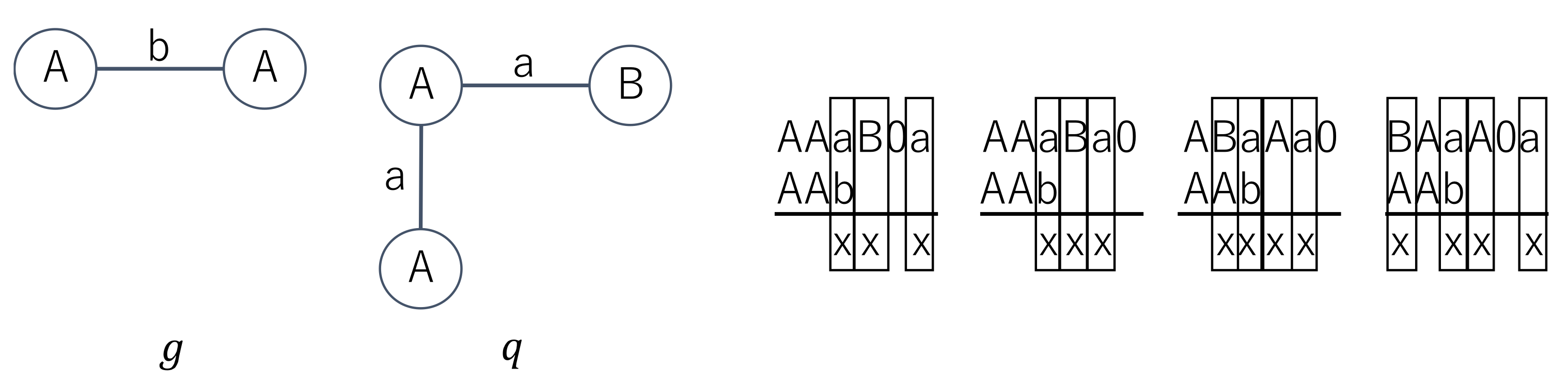
Example 2.

As shown in Figure 4, given two graphs g and q for which the edit distance is 3, let an arbitrary AcGM code of g be AAb. $\mathsf{\Omega }\left(q\right)$ is $\{AAaB0a,AAaBa0,ABaAa0,BAaA0a\}$. When the code AAb is compared with $AAaB0a\in \mathsf{\Omega }\left(q\right)$, we need three edits which are indicated as × in Figure 4. By comparing AAb and all elements in $\mathsf{\Omega }\left(q\right)$, we obtain the graph edit distance between q and g according to Lemma 10.

Figure 4. Computation of Graph Edit Distance using AcGM codes.

From Lemma 5, we have the following corollary.

Collorary 1.

If $ed(c,c^{\prime })\le \theta$ for two AcGM codes c and $c^{\prime }$, then $ed(g\left(c\right),g\left(c^{\prime }\right))\le \theta$.

Algorithm 1 shows the pseudocode for solving the problem defined by Equation (4). In Line 3, an arbitrary AcGM code from $\mathsf{\Omega }\left(g_i\right)$ is generated for graph $g_i$ in database G. After one of all possible AcGM codes for q is obtained in Line 4, a prefix $c^{\prime }$, which consists of j fragments $c_i$, is generated in Line 6. Since $c^{\prime }$ is a prefix of c, $g\left(c^{\prime }\right)$ must be a connected and is an induced subgraph of q. Subsequently, $g_i$ is added to the set of output graphs S if $ed(c_i,c^{\prime })\le \theta$, which indicates that $g_i$ is a solution in the set defined by Equation (4) according to Corollary 1. Once $g_i$ is added to S, any procedures for $g_i$ are stopped and procedures for the next graph $g_{i+1}$ are started. These steps are repeated for all of the graphs in G. The time complexity of Algorithm 1 is $O\left(\right|\mathsf{\Omega }\left(q\right)\left|{\sum }_{i=1}^{\left|G\right|}\right|V\left(g_i\right){|}^3)$ and the algorithm has some drawbacks, as follows.

(1)

Although the algorithm produces $\left|V\right(g_i\left)\right|$ prefixes in Line 6 for each AcGM code c in $\mathsf{\Omega }\left(q\right)$ and computes Equation (8) $\left|V\right(g_i\left)\right|$ times in Line 7 for the prefixes, some of the repeated calculations of Equation (8) are redundant because two prefixes $c^{\prime }$ and $c^{″}$ produced from c satisfy $c^{\prime }\subset c^{\prime \prime }$. Using the result of computing $ed(c_i,c^{\prime })$ to compute $ed(c_i,c^{″})$ would render Algorithm 1 efficient.

(2)

Let $G_c=\{code\left(g_i\right)\mid g_i\in G\}$ be the set of codes produced in Line 3. AcGM codes $code\left(g_i\right)$ and $code\left(g_j\right)$, for which their prefixes are the same, are included in $G_c$. The repeated calculations of Equation (8) between these AcGM codes and $c^{\prime }$ are redundant. If the common prefix of $code\left(g_i\right)$ and $code\left(g_j\right)$ is $c_s$, using the result of computing $ed(c_s,c^{\prime })$ to compute $ed(code\left(g_i\right),c^{\prime })$ and $ed(code\left(g_j\right),c^{\prime })$ would make Algorithm 1 efficient.

Algorithm 1: Straightforward Algorithm for Searching (4)

5. Method for Traversing Prefix Tree for Constrained Problem

In order to overcome drawback (1), described in the previous section, we introduce the following lemma.

Lemma 6.

Given two AcGM codes c and $c^{\prime }$, we have the following:

$$ed(pre(c,i),pre(c^{\prime },i))\le ed(pre(c,j),pre(c^{\prime },j))fori<j.$$

(11)

In the case that i is greater than the number of fragments in c, we assume that $pre(c,i)$ is equivalent to c itself.

Proof. 

$ed(pre(c,i+1),pre(c^{\prime },i+1))$ is the sum of $ed(pre(c,i),pre(c^{\prime },i))$ and the number of edits between the $i+1$-th fragments of $pre(c,i+1)$ and $pre(c^{\prime },i+1))$. Since the number of edits is non-negative, $ed(pre(c,i),pre(c^{\prime },i))$ increases monotonically when i is increased. Therefore, for $i<j$, we have $ed(pre(c,i),pre(c^{\prime },i))\le ed(pre(c,j),pre(c^{\prime },j))$. □

Collorary 2.

According to Lemma 6, if $ed(pre(c,i),pre(c^{\prime },i))>\theta$, then $ed(c,c^{\prime })>\theta$.

As a consequence of Lemma 6 and Corollary 11, when $ed(pre(c,i),pre(c^{\prime },i))>\theta$, we can stop the computation in Line 7 of Algorithm 1.

Lemma 7.

Given the two following fragments:

$$\begin{array}{ccc}\hfill s& =& \ell \left(u_i\right)x_{1,i}\cdots x_{i-1,i}\hfill \end{array}$$

(12)

$$\begin{array}{ccc}\hfill s^{\prime }& =& \ell \left(u_i^{\prime }\right)x_{1,i}^{\prime }\cdots x_{i-1,i}^{\prime },\hfill \end{array}$$

(13)

for which their lengths are equal, the number of edits $ed(s,s^{\prime })$ to equalize the fragments is as follows:

$$ed(s,s^{\prime })=\left\{\begin{array}{cc}1+{\displaystyle \sum _{1\le j<i}}{\delta }^{\prime }(0,x_{j,i}^{\prime })\hfill & (s=null)\hfill \\ 1+{\displaystyle \sum _{1\le j<i}}{\delta }^{\prime }(x_{j,i},0)\hfill & (s^{\prime }=null)\hfill \\ {\delta }^{\prime }(\ell \left(u_i\right),\ell \left(u_i^{\prime }\right))+{\displaystyle \sum _{1\le j<i}}{\delta }^{\prime }(x_{j,i},x_{j,i}^{\prime })\hfill & \left(otherwise\right).\hfill \end{array}\right.$$

(14)

Since $ed(s,s^{\prime })$ is a symmetric function, $ed(s,s^{\prime })=ed(s^{\prime },s)$.

Proof. 

Please see the proof for Lemma 3. □

Algorithm 2 shows the pseudocode for solving the problem defined by (4), which overcomes the aforementioned drawback (1). After obtaining the j-th fragments of AcGM codes $c_i$ and c in Line 7 of the algorithm, the number of edits between the fragments is calculated according to Lemma 7. The number of edits is then added to the accumulated edit count $ae$. According to Corollary 2, the algorithm stops the calculation of the number of edits between $c_i$ and one of the AcGM codes of q in Line 8. However, because $g_i$ is a member of the set defined in Equation (4) if the edited distance between $c_i$ and at least one AcGM code in $\mathsf{\Omega }\left(q\right)$ is less than $\theta$, these steps are repeated for all AcGM codes of q. The time complexity of Algorithm 2 is $O\left(\right|\mathsf{\Omega }\left(q\right)\left|{\sum }_{i=1}\left|G\right|\right|V\left(g_i\right){|}^2)$.

Algorithm 2: Straightforward Algorithm 2 for Searching (4)

In order to overcome drawback (2), described in the previous section, we use a prefix tree for the AcGM codes for G.

Definition 3

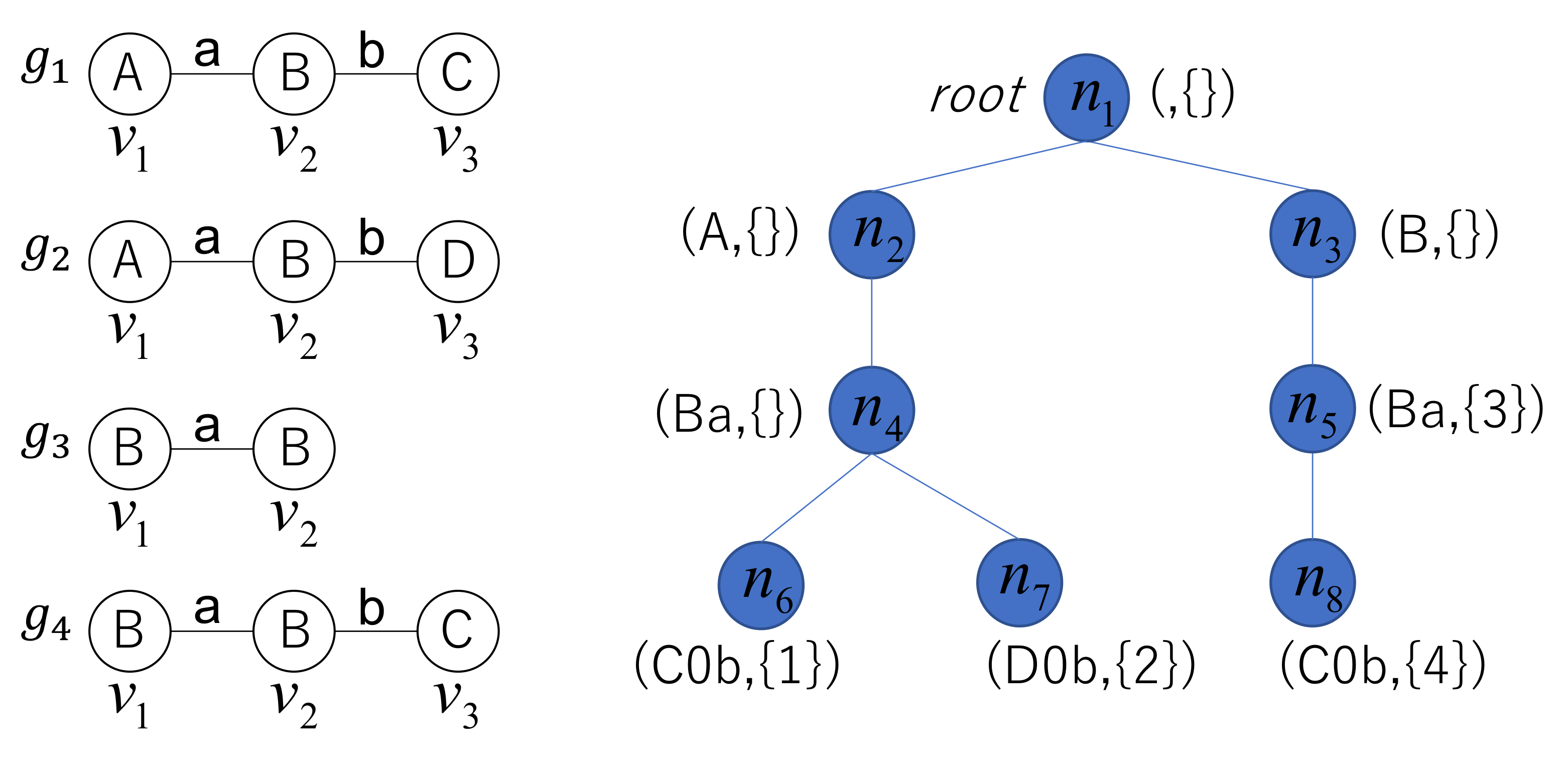
(Code Tree [17] (The detailed algorithm for constructing a code tree from a graph database G is given in [17].)). A code tree T is defined as the triplet $(\top ,N,B)$, where $\top \in N$ is the root node of the tree, N is a set of the nodes of the tree, and B is a set of the branches of the tree. In addition, each node is associated with a code fragment and a set of graph identifiers. Let $s\left(n\right)$ be the concatenation of the fragments associated with nodes on the path from the root to node n. When one of the AcGM codes of $g_i\in G$ is the same as $s\left(n\right)$, the set of graph identifiers for node n contains i, which is the identifier of graph $g_i\in G$.

The code fragment and graph identifiers associated with node n are denoted as $fr\left(n\right)$ and $ID\left(n\right)$, respectively. For the root node, $fr(\top )=null$ and $ID(\top )=\varnothing$. We present an example of a code tree below.

Example 3.

A graph database $G=\{g_1,g_2,g_3,g_4\}$ consists of four graphs, as shown in Figure 5. When one of the AcGM codes for each graph in G is generated, the AcGM codes for the four graphs are as follows.

$$\begin{array}{ccc}\hfill code(g_1,⟨v_1,v_2,v_3⟩)& =& ABaC0b,\hfill \\ \hfill code(g_2,⟨v_1,v_2,v_3⟩)& =& ABaD0b,\hfill \\ \hfill code(g_3,⟨v_1,v_2⟩)& =& BBa,and\hfill \\ \hfill code(g_4,⟨v_1,v_2,v_3⟩)& =& BBaC0b.\hfill \end{array}$$

Figure 5. Code tree.

From these AcGM codes, a code tree is constructed, as shown in the right part of Figure 5. Node $n_6$ of the tree is associated with the code fragment $C0b$ and the set of graph identifiers $ID\left(n\right)=\left\{1\right\}$. The concatenation of fragments associated with nodes on the path from the root to node $n_6$ is $ABaC0b$, which represents graph $g_1$ in G.

Algorithm 3 shows the pseudocode for searching for members of the set defined in Equation (4) by traversing the code tree. At node n, Algorithm 3 adds vertex w of q to $⟨w_1,w_2,\dots ,w_h⟩$, from which the fragment s is generated, with the addition of the prefix $code(q,⟨w_1,w_2,\dots ,w_h⟩)$ of an AcGM code of q. The algorithm then recursively traverses the children of n that have fragments similar to fragment s. In contrast to Algorithm 2, which iteratively checks whether each individual graph in the graph database is a solution, Algorithm 3 checks whether multiple graphs in the database are simultaneously solutions. This is because each node in the code tree is associated with the common prefix of the AcGM codes of multiple graphs in the database. This simultaneous checking renders our search very efficient. The worst case time complexity of Algorithm 3 is the same as the time complexity of Algorithm 2. When AcGM codes of graphs in the database do not have common prefixes as one another, the time complexity of Algorithm 3 becomes worst. However, the codes usually have common prefixes as one another and the computation time that this algorithm needs is proportional to the number of nodes that Algorithm 3 traverses. In addition, at each node, Algorithm 3 needs $O\left(h\right|V\left(q\right)\left|\right|N\left|\right)$.

Algorithm 3: Code Tree Search for Finding Solutions to Equation (4)

6. Method for Traversing Prefix Tree for Original Problem

At node n, for which its depth is h in the code tree, Algorithm 3 retains the accumulated edit count $ae$ for two concatenations c and $c^{\prime }$ of fragments of length h. c and $c^{\prime }$ have the following restrictions:

• c is a concatenation of fragments associated with nodes on the path from the root of the code tree to n and is an AcGM code of a connected and induced graph that is a common subgraph of multiple graphs in the graph database;
• $c^{\prime }$ is a prefix of one of the AcGM codes in $\mathsf{\Omega }\left(q\right)$. According to the definition of the AcGM code, $g\left(c^{\prime }\right)$ must be connected and is an induced subgraph of q.

In order to solve the original problem for searching for solutions to Equation (3), we relax the restrictions as follows. The restriction that $g\left(c^{\prime }\right)$ is connected is a consequence of the fact that $code(q,⟨w_1,w_2,\dots ,w_h⟩)$ is a prefix of the AcGM codes $\mathsf{\Omega }\left(q\right)$ of q. Therefore, in Line 4 of Algorithm 3., we relax this restriction by allowing $⟨w_1,w_2,\dots ,w_h⟩$ to be all possible h-permutations of $vertices\{v_1,v_2,\dots ,v_{\left|V\right(q\left)\right|}\}$ in q. Codes $code(q,⟨w_1,w_2,\dots ,w_h⟩)$ by some of the permutations correspond to unconnected graphs.

Next, we relax the restriction that $g\left(c^{\prime }\right)$ is an induced subgraph of q. Algorithm 1 produces prefixes of the AcGM codes of q to obtain connected and induced subgraphs of q. Suppose that we would like to obtain, in addition to the connected and induced subgraphs, all possible unconnected and non-induced subgraphs of q. In this case, we may need, in addition to the prefixes of the AcGM codes of q, all possible codes generated by replacing some elements $x_{i,j}$ in the prefixes by 0. 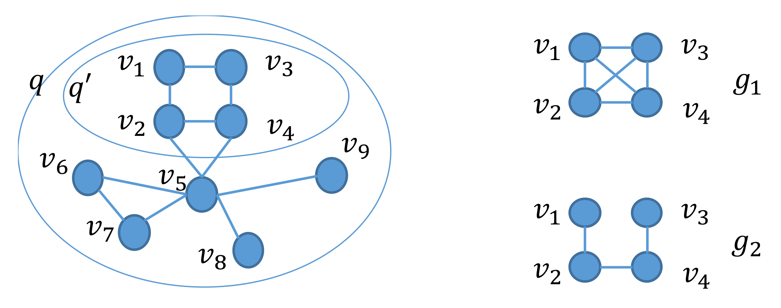This requires us to solve both the permutation problem among the vertices of q and the combination problem among the edges of q. However, we do not need to solve the latter problem for the following reasons. We consider a graph q, its induced subgraph $q^{\prime }$, and two graphs $g_1$ and $g_2$, shown in Figure 6. We refer to two vertices in $q^{\prime }$ as $v_i$ and $v_j$.

Figure 6. Inclusion of graphs and similarity.

• $ed(q^{\prime },g_1)=2$. Given a graph $q^{″}$ obtained by removing an edge from $q^{\prime }$, we have $ed(q^{\prime },g_1)<ed(q^{″},g_1)=3$. In the problem of finding solutions to Equation (3), we check whether there exists a subgraph of q such that $ed(q^{\prime },g_i)\le \theta$ and this subgraph need not be an induced subgraph of q. Therefore, in the case that there is an edge between two vertices $v_i$ and $v_j$ in $q^{\prime }$ and there is also an edge in $g_i$ between the two corresponding vertices, we do not need to consider the graph $q^{″}$ obtained by removing an edge from $q^{\prime }$. That is, we do not need to replace any elements $x_{i,j}$ in prefixes of the AcGM codes of $q^{\prime }$ by 0.
• $ed(q^{\prime },g_2)=1$. For the above $q^{″}$, we have $ed(q^{\prime },g_2)>ed(q^{″},g_2)=0$. Therefore, in the case that there is an edge between two vertices $v_i$ and $v_j$ in $q^{\prime }$ and there is no edge in $g_i$ between the two corresponding vertices, we do not need to consider the graph that does not have an edge corresponding to edge $(v_i,v_j)$ in $q^{\prime }$.
• In all other cases, there is no edge between $v_i$ and $v_j$ in $q^{\prime }$. Since $x_{i,j}=0$, we do not need to replace $x_{i,j}$ by 0.

From the above discussion, we rewrite Lemma 7 as follows.

Lemma 8.

$ed(s,s^{\prime })$

$$=\left\{\begin{array}{cc}1+{\displaystyle \sum _{1\le j<i}}{\delta }^{\prime }(x_{j,i},0)\hfill & (s^{\prime }=null)\hfill \\ 1\hfill & (s=null)\hfill \\ {\delta }^{\prime }(\ell \left(v_i\right),\ell \left(v_i^{\prime }\right))+{\displaystyle \sum _{\begin{array}{c}1\le j<i\\ x_{i,j}\ne 0\end{array}}}{\delta }^{\prime }(x_{j,i},x_{j,i}^{\prime })\hfill & (s\ne null\wedge s^{\prime }\ne null).\hfill \end{array}\right.$$

(15)

This function is asymmetric.

Since we consider all possible subgraphs of q by the function defined in Equation (8), we need to produce only the prefixes underlined above.

Algorithm 4 shows the pseudocode for searching for members of the set defined in Equation (3) by traversing the code tree. The part from Lines 4–9 searches $\{g_i\in G\mid q^{\prime }\subseteq qs.t.ed(q^{\prime },g_i)\le \theta ,|V\left(g_i\right)|\le |V\left(q^{\prime }\right)\left|\right\}$, whereas the part from Lines 10–13 searches $\{g_i\in G\mid q^{\prime }\subseteq qs.t.ed(q^{\prime },g_i)\le \theta ,|V\left(g_i\right)|>|V\left(q^{\prime }\right)\left|\right\}$. The other difference between Algorithm 3 and Algorithm 4 is Line 4, which produces codes from one of all possible h-permutations of vertices of the query graph q. The codes produced are not limited to AcGM codes, but are AGM codes [24]. In Lines 7 and 11, Equation (15) is used to calculate the similarity between two fragments. Since the codes produced in Line 4 are limited to prefixes of the AGM codes of q, we do not need to solve the combination problem among the edges of q, which enables our proposed method to be very efficient. The time complexity of Algorithm 4 is the same as one of Algorithm 3; nevertheless, the problem that Algorithm 3 solves is a constrained problem of the problem that Algorithm 4 solves.

Algorithm 4: Code Tree Search for Finding Solutions to Equation (3)

7. Customization of Solutions

In the previous section, we proposed a method for searching for the set of graphs S defined by Equation (3). The number of graphs reachable by editing graph $q^{\prime }$$\theta$ times in Equation (3) increases exponentially as $\theta$ is increased. Therefore, for a large $\theta$, the computation time required to search for the graphs in S becomes excessively long. However, some real applications need to obtain the following sets of constrained graphs rather than obtaining all the graphs in S.

$⟨1⟩$

Editing graphs is constrained: for example, the relabeling of vertices or edges is admissible in $ed(q^{\prime },g_i)$ of Equation (3), whereas insertions and deletions are not admissible. That is, when converting a labeled graph g to an unlabeled graph $un\left(g\right)$ by removing label information from vertices and edges in g, $un\left(g_i\right)$ and $un\left(q^{\prime }\right)$ in Equation (3) are isomorphic.

$⟨2⟩$

Editing graphs is constrained: for example, editing some specific vertices and edges in a query graph q is admissible, whereas editing other vertices and edges is not admissible. For example, in the substructure drawn with blue lines and labels in Figure 1, editing its ring structure is admissible, whereas editing the remainder of the blue substructure is not admissible.

The problem for the above constraint $⟨1⟩$ is formalized as follows.

$$\{g_i\in G\mid \exists q^{\prime }\subseteq qs.t.ed(g_i,q^{\prime })\le \theta \wedge un\left(g_i\right)=un\left(q^{\prime }\right)\}.$$

(16)

In order to solve this problem, Equation (15) is rewritten as follows.

$$\begin{array}{ccc}& & ed(s,s^{\prime })\hfill \\ & =& \left\{\begin{array}{cc}{\delta }^{\prime }(\ell \left(v_i\right),\ell \left(v_i^{\prime }\right))+{\displaystyle \sum _{\begin{array}{c}1\le j<i\\ \wedge x_{i,j}\ne 0\\ \wedge x_{i,j}^{\prime }\ne 0\end{array}}}{\delta }^{\prime }(x_{j,i},x_{j,i}^{\prime })+{\displaystyle \sum _{\begin{array}{c}1\le j<i\\ \wedge (x_{i,j}=0\\ \vee x_{i,j}^{\prime }=0)\end{array}}}\infty \hfill & (s\ne null\wedge s^{\prime }\ne null)\hfill \\ \infty \hfill & \left(otherwise\right).\hfill \end{array}\right.\hfill \end{array}$$

(17)

For the case of $s\ne null\wedge s^{\prime }\ne null$, the first and second terms in Equation (17) are the numbers of edits that occur by relabeling the i-th vertices and edges $(i,j)(1\le j<i)$, respectively, in $g\in G$ and $q^{\prime }$. The third term of Equation (17) is the sum of the numbers of edits that occur by inserting or deleting edges. For this case, in containing such insertion or deletion operations, the $ed(s,s^{\prime })$ function returns values larger than $\theta$ and Algorithm 4 (in Line 7) backtracks the code tree.

For the case of the above constraint $⟨2⟩$, let some specific vertices in query graph q be $V_q\subseteq V\left(q\right)$. When Algorithm 4 visits node n in the code tree, it generates various codes by $⟨w_1,w_2,\dots ,w_h,w⟩$, in Line 4. Some vertices in $⟨w_1,w_2,\dots ,w_h,w⟩$ are included in $V_q$, but others are not. In this case, Equation (15) is rewritten as follows.

$$\begin{array}{ccc}& & ed(s,s^{\prime })\hfill \\ & =& \left\{\begin{array}{cc}{\delta }^{\prime }(\ell \left(v_i\right),\ell \left(v_i^{\prime }\right))+{\displaystyle \sum _{\begin{array}{c}{w}_j\in V_q\\ \wedge 1\le j<i\\ \wedge x_{i,j}\ne 0\end{array}}}{\delta }^{\prime }(x_{j,i},x_{j,i}^{\prime })+{\displaystyle \sum _{\begin{array}{c}{w}_j\notin V_q\\ \wedge 1\le j<i\\ \wedge x_{i,j}\ne 0\end{array}}}\infty \hfill & (s,s^{\prime }\ne null\wedge w_i\in V_q)\hfill \\ \infty \hfill & \left(otherwise\right).\hfill \end{array}\right.\hfill \end{array}$$

(18)

Thus, for the case of $s\ne null\wedge s^{\prime }\ne null\wedge w_i\in V_q$, the first and second terms of Equation (18) are the numbers of edits that occur by relabeling the i-th vertices and edges $(i,j)(1\le j<i)$, respectively, in $g\in G$ and $q^{\prime }$, where $w_i$ and $w_j$ are elements in $V_q$. The third term of Equation (18) is the sum of the numbers of edits that occur by editing the other vertices and edges.

In order to summarize the above discussion, the advantages of our proposed method are the following:

• Users can search for their desired type of similar graphs in a database containing graphs;
• This search can be realized by simply rewriting Equation (15), without the need to modify Algorithm 4.

Therefore, the method proposed in this paper is a general and flexible framework for searching for similar subgraphs of query graphs and is easily customizable for searching for the types of graphs desired by the user.

8. Experimental Evaluation

For our experimental evaluation, we used the three real-world datasets used in [18] which were downloadable from https://github.com/SNUCSE-CTA/IDAR on 1 March 2021. The datasets consisting of chemical compounds are called AIDS, NCI, and PubChem. Each atom, chemical bond, atom type, and bond type in a chemical compound corresponds to a vertex, edge, vertex label, and edge label, respectively. Sets of queries and databases containing graphs were generated from each of the datasets. One hundred query graphs, each containing more than 100 vertices, were selected from each of the datasets. Each generated database contained between 10,000 and 100,000 graphs and each of the graphs was generated by one of two different methods [18]. In the first method, each graph in a database consisted of vertices and edges on a random walk on a graph randomly selected from one of the datasets. This type of database is called rand. In the second method, each graph in a database was a frequent subgraph with a minimum support value of 0.1% [24] that is enumerated from one of the datasets. This type of database is called freq. In the experiments, vertices corresponding to hydrogen were removed, which is similar to the experiments in [2,14,17,30]. Table 2 summaries graphs in databses and queries in our experiments.

Table 2. Summary of datasets used in our experiments.

	AIDS		NCI		PubChem
	Rand	Freq	Rand	Freq	Rand	Freq
# of vertex labels	31	10	42	15	16	9
# of edge labels	3	3	3	3	3	2
graphs in databases
# of graphs	100,000	100,000	100,000	100,000	100,000	100,000
avg. # of vertices	29.0	21.4	28.2	16.9	27.6	24.1
max. # of vertices	100	26	79	27	84	32
min. # of vertices	1	10	1	5	1	11
avg. # of edges	30.0	20.4	29.2	16.1	28.2	23.1
query graphs
# of graphs	100		100		100
avg. # of vertices	71.0		63.9		64.9
max. # of vertices	222		132		175
min. # of vertices	42		40		34
avg. # of edges	74.9		68.9		67.8

Since the problem of similar supergraph search is a novel problem proposed in this paper, there are no methods for solving this problem other than our proposed method to the best of our knowledge. Although we cannot compare our proposed method with other methods, our method is based on CodeTree (We use “CodeTree” to name the method proposed in [17] and “code tree” to represent the index used in CodeTree). This is proposed in [17] and our method with $\theta =0$ is equivalent to CodeTree. Our proposed method was implemented in Java and the experiments reported in this section were conducted on a workstation with an AMD Ryzen Threadripper 3970X 3.7 GHz CPU and 64 GB main memory.

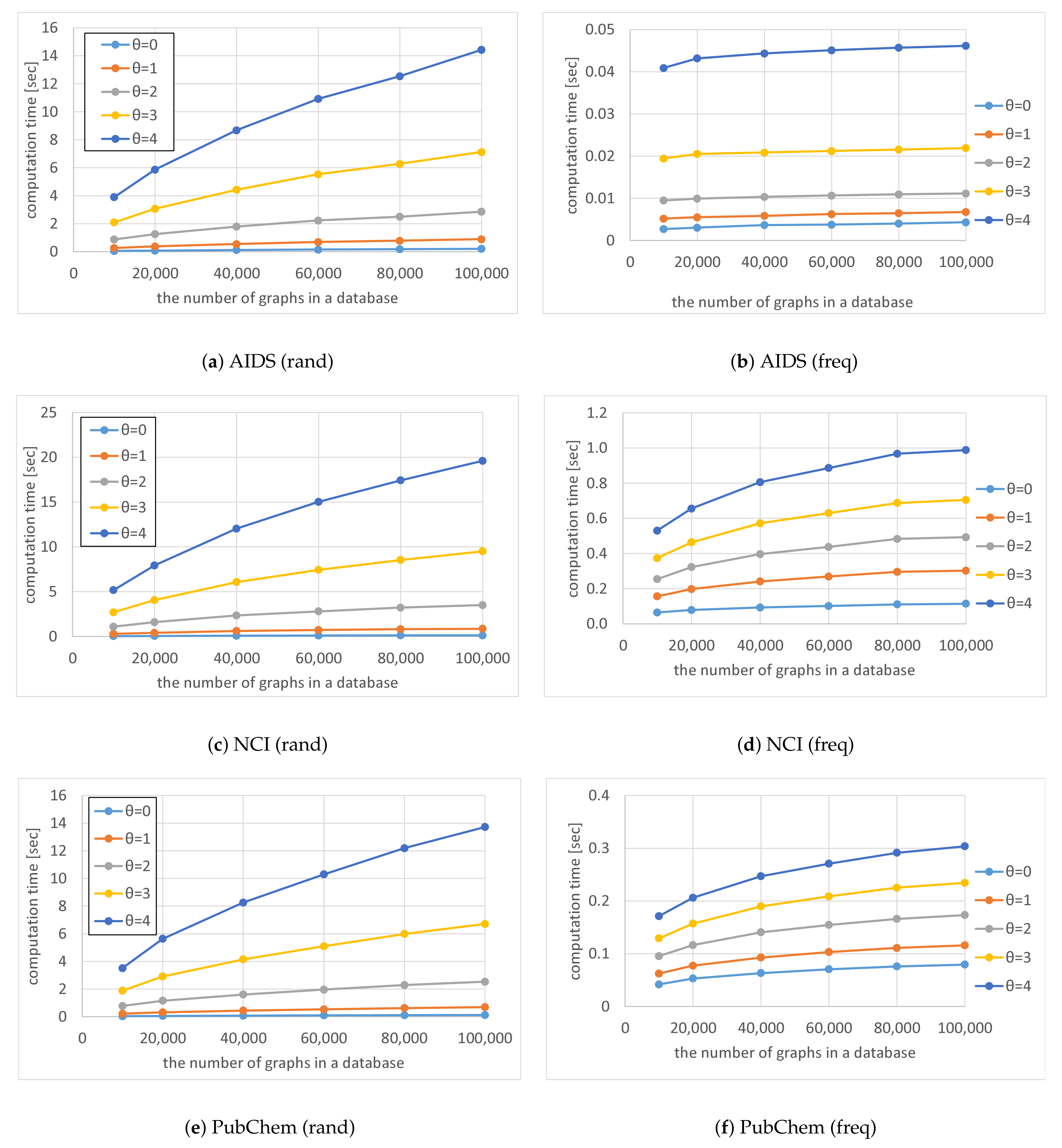
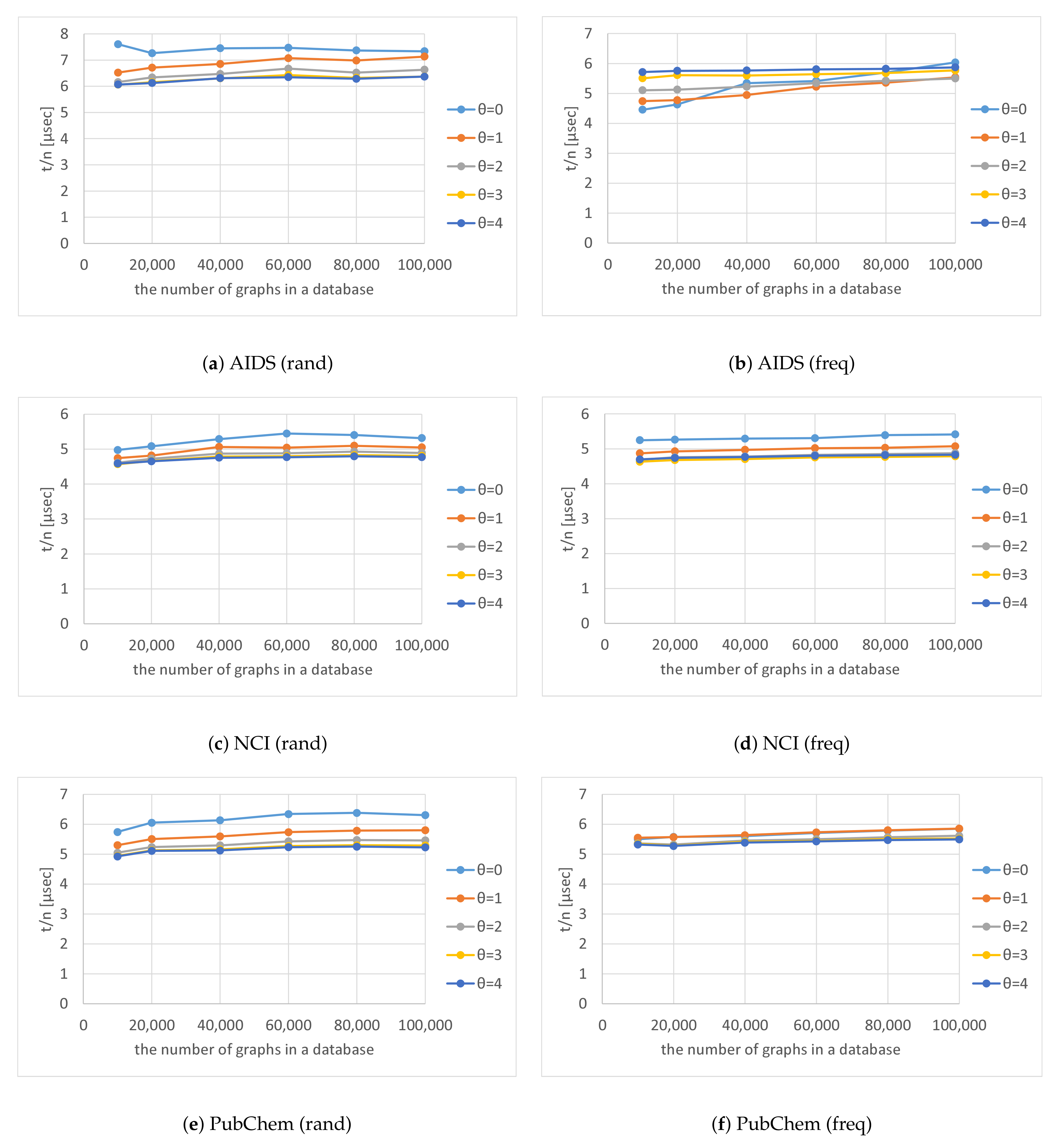
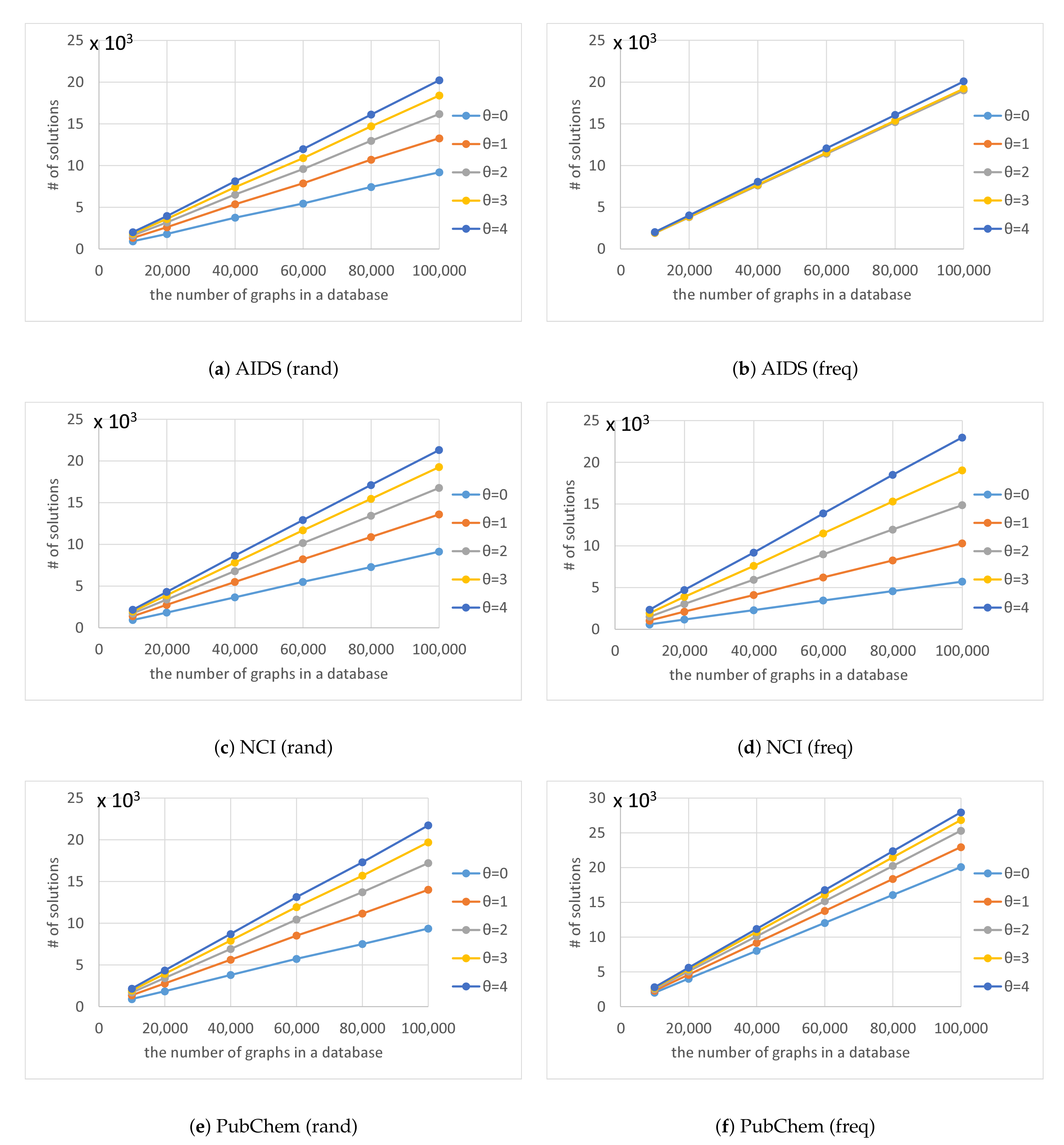
First, we conducted experiments for Algorithm 4 with Equation (17). Figure 7, Figure 8 and Figure 9 show the average computation time (query processing time) t, the average number of nodes n in the code tree that our method traversed, and the average number of solutions $\left|S\right|$, respectively, for various numbers of graphs $\left|G\right|$ in a database and various thresholds $\theta$. The computation time increased as the number of graphs in a database increased, as shown in Figure 7. Although the time complexity of Algorithms 1 and 2 is linearly related to the number of graphs in the database, the computation time of our method was sublinear for the number of graphs in the database because Algorithm 4 maintains the correspondence between a vertex of a query graph and vertices of multiple graphs in the database simultaneously. In contrast, the computation time increased exponentially as $\theta$ was increased, as shown in Figure 7. This is because the number of graphs reachable by editing a graph $q^{\prime }\subseteq q$$\theta$ times increases exponentially. Although the computation time increased as the database size increased for freq databases, the rate of increase was less than for rand databases. 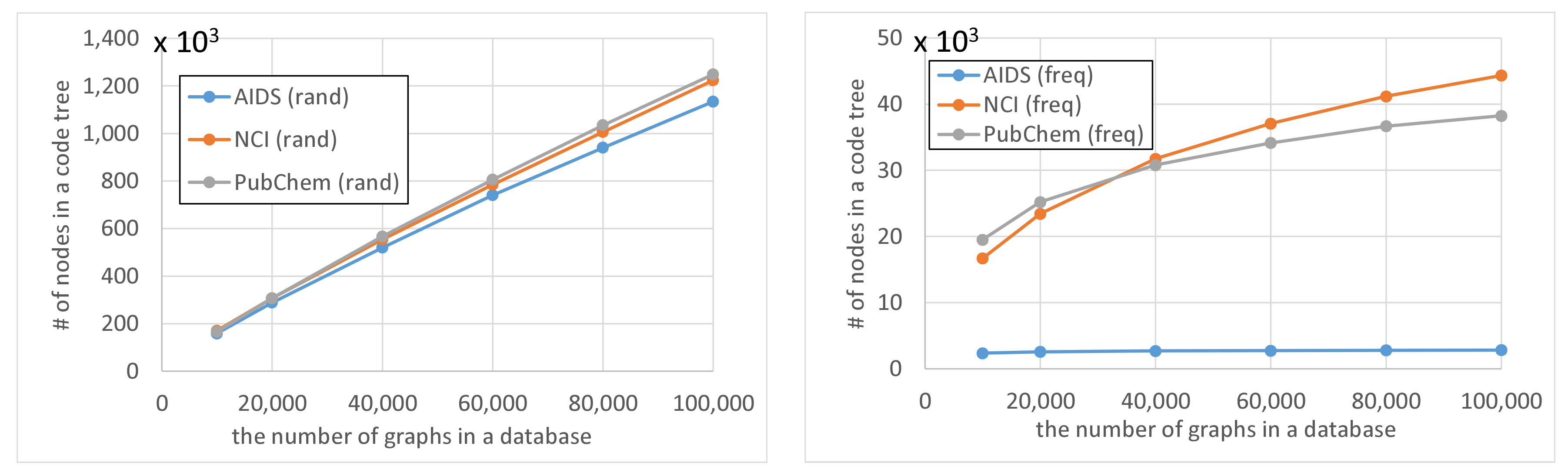This is because the numbers of nodes in code trees for freq databases are smaller than those for rand databases and the former numbers are relatively unchanged by the increase in database size, as shown in Figure 10. The reason why the numbers of nodes in code trees are largely unaffected by database size is that frequent subgraphs enumerated from the datasets are similar to each other and the AcGM codes of similar frequent subgraphs have common prefixes. This is because a subgraph of a frequent subgraph is also a frequent subgraph, which is a consequence of the anti-monotonic property of the support value [24].

Figure 7. Average computation times t for various numbers of graphs $\left|G\right|$ in a database and various thresholds $\theta$.

Figure 8. Average numbers of nodes n in the code tree that our method traversed for various numbers of graphs $\left|G\right|$ in a database and various thresholds $\theta$.

Figure 9. Number of solutions $\left|S\right|$ for various numbers of graphs $\left|G\right|$ in a database and various thresholds $\theta$.

Figure 10. Number of nodes in code trees.

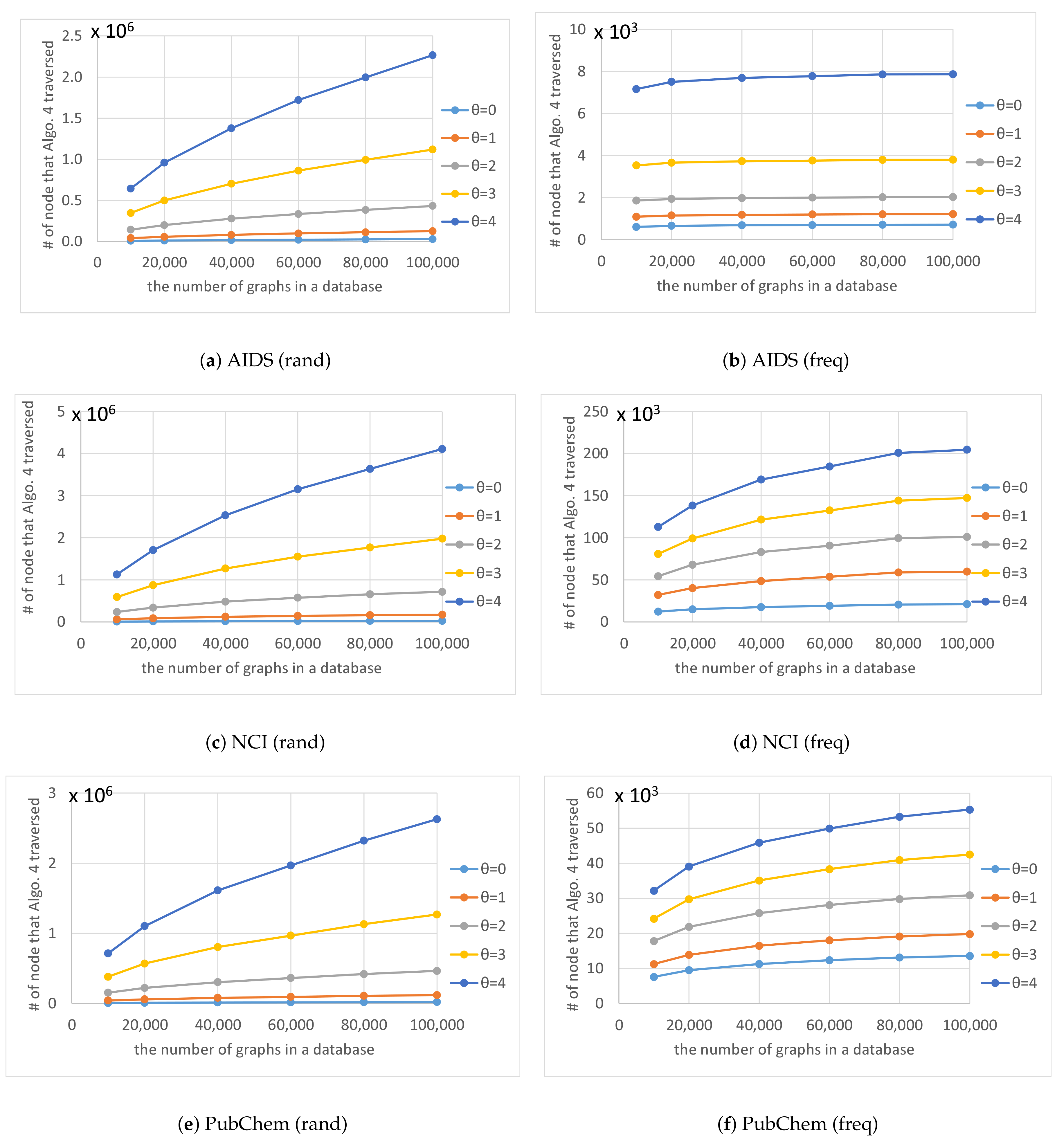
As shown in Figure 8, the number of nodes in the code tree that Algorithm 4 traversed also increased exponentially as $\theta$ increased. The shapes of the curves plotted in Figure 8 are similar to those in Figure 7 and the trend for the numbers $\left|G\right|$ of graphs in databases and thresholds $\theta$ in Figure 8 are also similar to those in Figure 7. Figure 11 shows $t/n$ for various numbers of graphs $\left|G\right|$ in a database and various thresholds $\theta$. 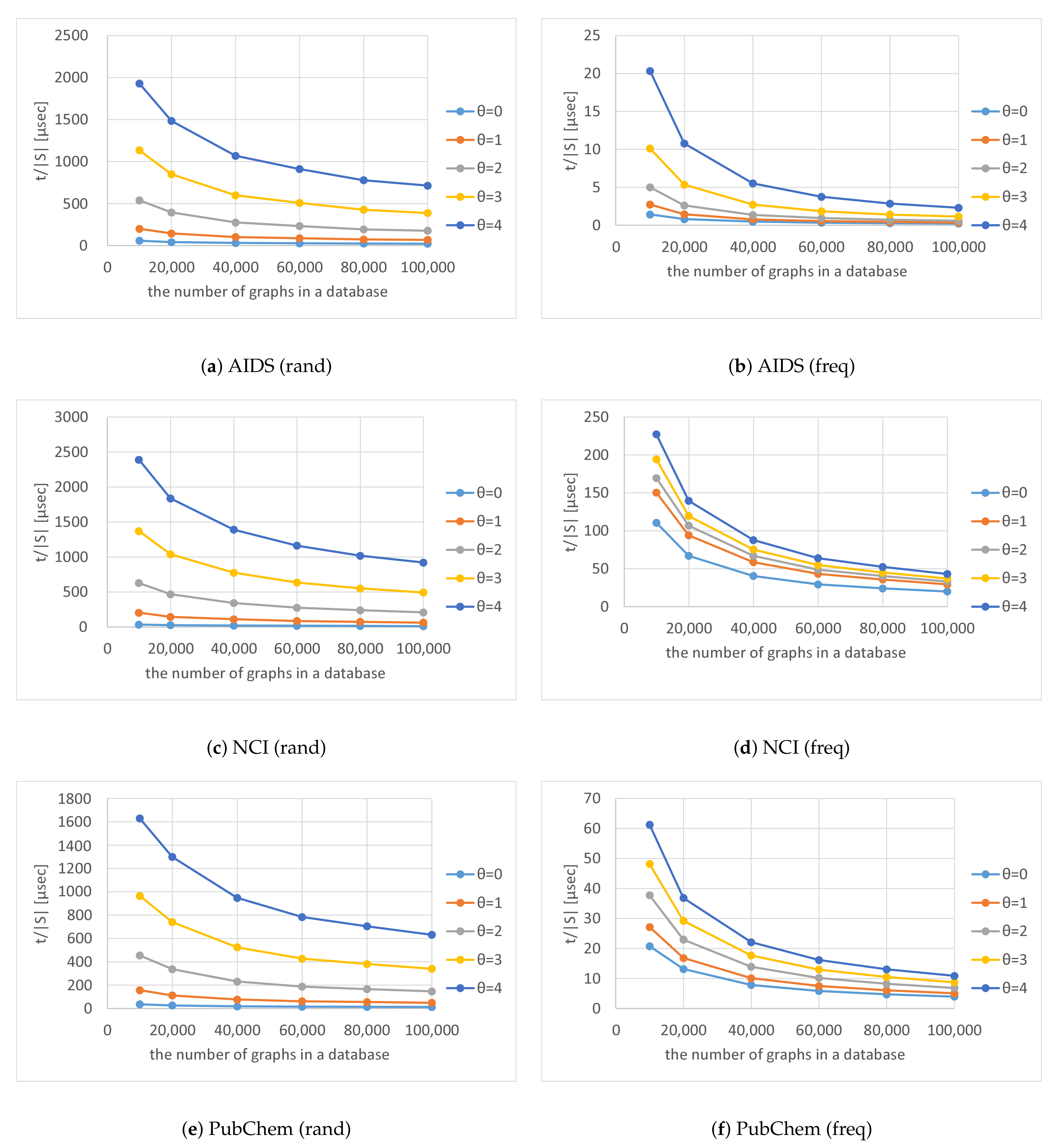The figure shows that $t/n$ is almost constant and unaffected by the number of graphs in a database, which indicates that the computation time of our method is proportional to the number of nodes in the code tree that Algorithm 4 traverses.

Figure 11. Computation time per node $t/n$ for various numbers of graphs $\left|G\right|$ in a database and various thresholds $\theta$.

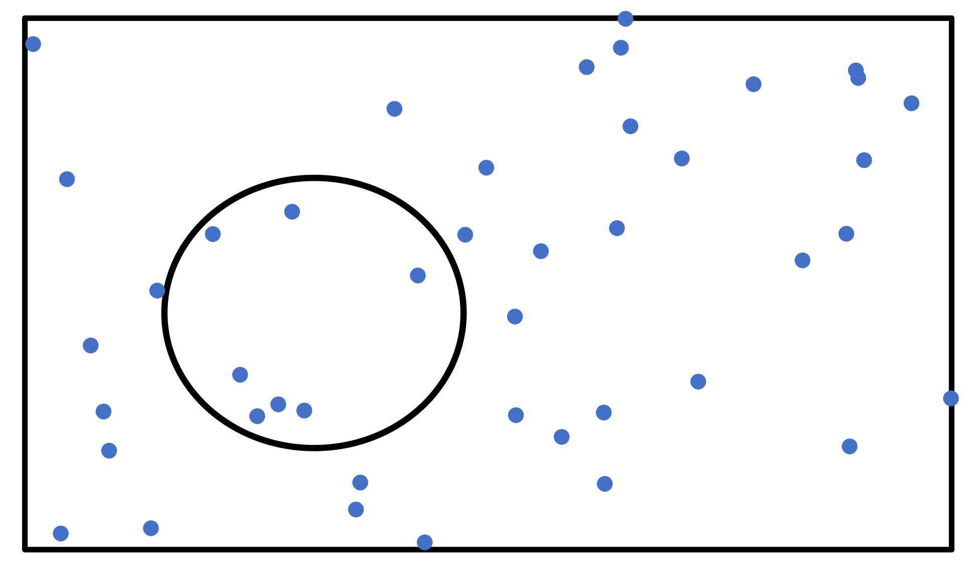
As shown in Figure 9, the number of solutions found by Algorithm 4 was proportional to the number of graphs in the databases. Because there is a limit to the number of graphs in the database, the number of solutions did not increase exponentially as $\left|G\right|$ increased. The rectangle in Figure 12 shows the space in which graphs in a database are distributed and each point in the rectangle shows a graph in the database. Points inside the circle are solutions for a given query q and threshold $\theta$. If the number of graphs in database G is doubled to $G^{\prime }$, such that $2\left|G\right|=|G^{\prime }|$, the number of points surrounded by the circle doubles, if the distribution is not changed such that $\mathcal{P}\left(G\right)=\mathcal{P}\left(G^{\prime }\right)$. Thus, the number of solutions found by Algorithm 4 is proportional to the numbers of graphs in the databases.

Figure 12. Distribution of graphs in a database.

Figure 13 shows $t/\left|S\right|$ for various numbers of graphs $\left|G\right|$ in a database and various thresholds $\theta$; the figure indicates the average computation time to output each solution. As the numbers of graphs in the databases increased, $t/\left|S\right|$ decreased exponentially. This is because $\left|S\right|$ is proportional to the number of graphs in a database, whereas the overall computation time to search for solutions is sublinear.

Figure 13. Computation time per solution $t/\left|S\right|$ for various numbers of graphs $\left|G\right|$ in a database and various thresholds $\theta$.

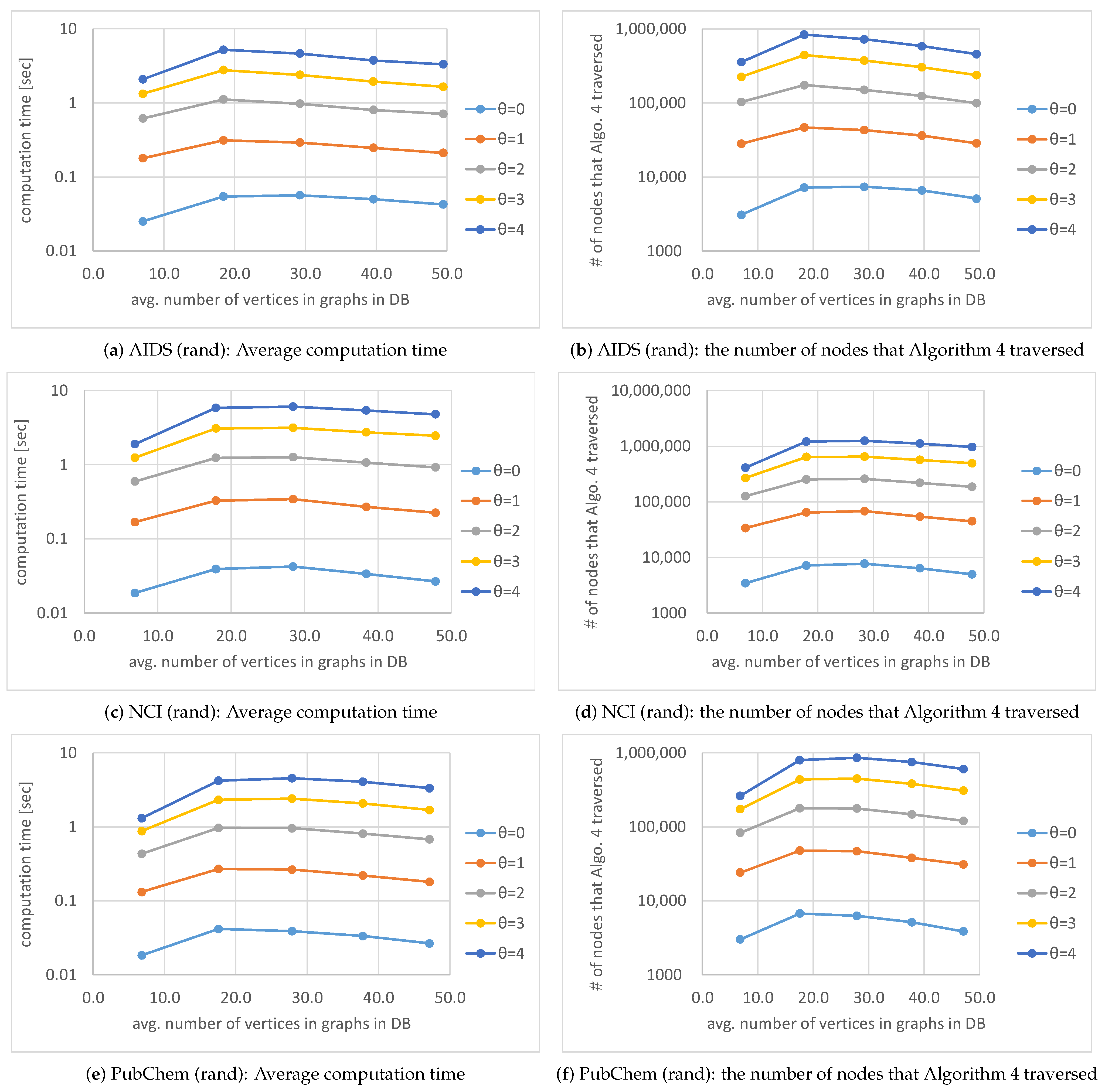
Figure 14 shows that average computation time and the number of nodes that Algorithm 4 traversed for various average numbers of vertices in graphs in a database and various thresholds $\theta$. When the average number of vertices in graphs in a database is increased, the average computation time of Algorithm 4 is largely unaltered because the computation time of Algorithm 4 is proportional to the number of nodes that Algorithm 4 traverses, as mentioned after Algorithm 3. The number is also largely unaltered with respect to the change of the average number of the vertices. The reason why the number of nodes that Algorithm 4 traversed is largely unaltered is because of the use of the function $ed(s,s^{\prime })$ shown in Equation (17). By using Equation (17), the relabeling of vertices or edges is admissible, whereas insertions and deletions of the vertices and edges are not admissible. Therefore, nodes that Algorithm 4 traverses are restricted. As mentioned in Section 7, one of the advantages of our proposed method is the customizability for searching for the types of graphs desired by users. By customizing the search for the types of graphs, the users can reduce not only the number of solutions to be outputted but also computation time of our proposed method.

Figure 14. Average computation time and the average number of nodes that Algorithm 4 traversed for various numbers of vertices in graphs in a database and various thresholds $\theta$.

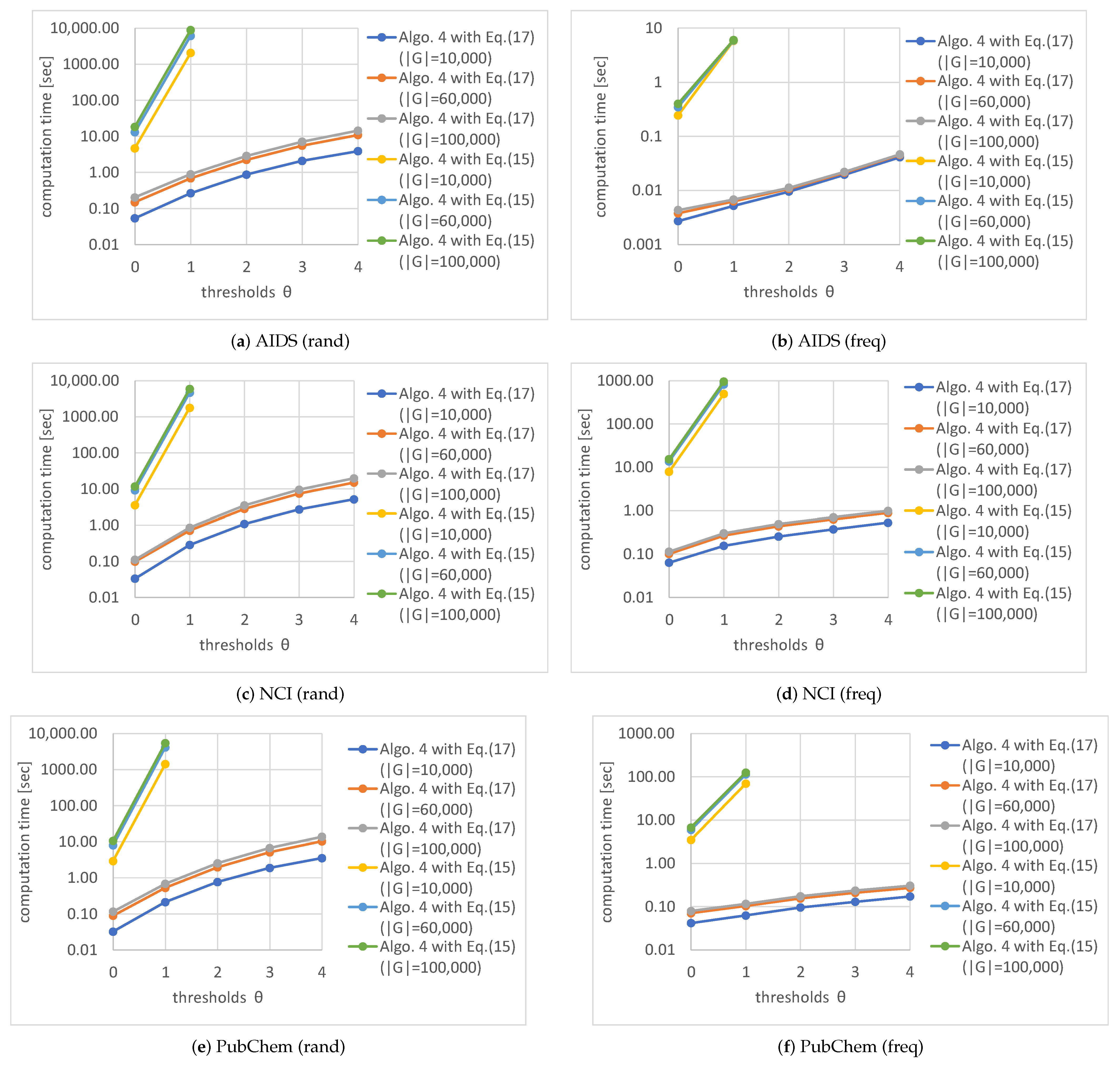
Next, we conducted experiments for Algorithm 4 with Equations (15) and (17). Figure 15 shows the computation times for various numbers of graphs in the databases and various thresholds. The computation times with Equation (17) were much shorter than those with Equation (15). This is because the number of graphs reachable by editing a graph $q^{\prime }\subseteq q$$\theta$ times increases exponentially and editing graphs with Equation (17) is limited to the relabeling of vertices and edges, which is faster than the insertion and deletion of vertices and edges that are required with Equation (15).

Figure 15. Computation times of Algorithm 4 with Equation (15) and Equation (17) for various numbers of graphs $\left|G\right|$ in a database and various thresholds $\theta$.

9. Conclusions

In this paper, we proposed a novel problem, which is called similar supergraph search, and designed an efficient algorithm to solve the problem. The problem is to identify all graphs in a database that are similar to any subgraph of a query graph, where similarity is defined as the edit distance. The proposed algorithm has three advantages for searching a database consisting of graphs for similar graphs. The first advantage is that the algorithm checks whether multiple graphs in the database are simultaneously solutions, because each node in the code tree is associated with the common prefix of the AcGM codes of multiple graphs in the database. The second advantage is that the codes produced by our proposed algorithm are limited to prefixes of the AGM codes of q and we do not need to solve the combination problem among the edges of q. The third advantage is the customization that enables users to search for their desired type of similar graphs in a database containing graphs. Therefore, the algorithm is a general and flexible framework for searching for similar subgraphs of query graphs and it is easily customizable for searching for the types of graphs desired by the user. Our experiments showed that the computation time increased exponentially as the distance threshold increased, but increased sublinearly with the number of graphs in the database.