Boundary Loss-Based 2.5D Fully Convolutional Neural Networks Approach for Segmentation: A Case Study of the Liver and Tumor on Computed Tomography

Abstract

Image segmentation plays an important role in the field of image processing, helping to understand images and recognize objects. However, most existing methods are often unable to effectively explore the spatial information in 3D image segmentation, and they neglect the information from the contours and boundaries of the observed objects. In addition, shape boundaries can help to locate the positions of the observed objects, but most of the existing loss functions neglect the information from the boundaries. To overcome these shortcomings, this paper presents a new cascaded 2.5D fully convolutional networks (FCNs) learning framework to segment 3D medical images. A new boundary loss that incorporates distance, area, and boundary information is also proposed for the cascaded FCNs to learning more boundary and contour features from the 3D medical images. Moreover, an effective post-processing method is developed to further improve the segmentation accuracy. We verified the proposed method on LITS and 3DIRCADb datasets that include the liver and tumors. The experimental results show that the performance of the proposed method is better than existing methods with a Dice Per Case score of $74.5\%$ for tumor segmentation, indicating the effectiveness of the proposed method.

1. Introduction

Image segmentation is a fundamental task in computer vision. It plays an important role in medical imaging technology, material science and other fields. Typical approaches for image segmentation include intensity thresholds [1], region growing [2], deformable models [3] and some methods based on machine learning. However, these methods over rely on predefined characteristics, which makes it difficult to automated medical image segmentation tasks. Recently, many deep learning methods have been proposed to automatically segment medical images [4,5]. For instance, He et al. [6] proposed a residual learning framework to improve accuracy by $28\%$ on common objects in context (COCO) dataset, which compared with previous methods. Moreover, Long et al. [7] constructed an end-to-end fully convolutional network, which could input an image of any size and could output the corresponding segmentation results. This method improved performance on the visual object classes (VOC) dataset [8] by $20\%$.

Generally, deep learning methods can be classified into three categories based on the dimension of input data: (1) 2D models: Cascaded-FCNs [9], and VGG based on fully convolutional network (FCN) [10]; (2) 3D models: ConVNet based densely connected convolutional networks [11], 3D FCN [12] and 3D U-Net [13]; and (3) 2.5D models: U-Net based residual networks [14] and recursive neural networks (RNNs) based on intra-slice features [15]. In general, a 2D model inputs a preprocessed image and outputs a probabilistic map. The 3D model can be regarded as an enhancement of the 2D model, which inputs a series of adjacent images with related information and outputs a corresponding set of probabilistic maps. Different from 2D and 3D models, the 2.5D model inputs several adjacent images with related information and outputs the probability map in the middle of these images. Although the current deep learning methods have improved the performance of automated segmentation of 3D medical images, they still have some problems and need to be improved. For example, the previous 2D FCNs [9,16,17] ignore the context information between the slices in the z-axis direction, which results in low segmentation accuracy. On the other hand, the effect of the 2.5D network on the fuzzy boundary segmentation of the medical images was not sufficient [14]. In addition, the training of 3D networks requires higher hardware configurations and more computational resources. With the same computational resources, the larger number of parameters and computational consumption from 3D networks limit the design of deeper and more complex network structures. For instance, Li et al. [18] used 3D network structures to segment 3D medical images, and used 24G video random access memory (VRAM) to train and test their networks.

Moreover, the loss function is also key for the optimization of the deep learning model. For the medical segmentation tasks, cross-entropy [19], similarity coefficient [20] and contour [21] are usually used as loss functions. These loss functions tend to focus on feature extraction in a specific region and lack the ability to learn features with fuzzy boundary information since the boundary includes very important feature information for image processing. With deep learning models, the learning of boundary information can improve the performance of image segmentation. To learn more about the boundary information for medical image segmentation, a boundary loss function is introduced into the proposed 2.5D deep learning model.

Here, we perform segmentation of the liver and tumors in contrast-enhanced computed tomography (CT) as experimental cases. The liver is one of the most important organs in the human body and it can assist in the digestion of food and the breakdown of toxic substances [22,23]. Liver cancer is known as the sixth most common cancer in the world and is one of the most common cancers [24]. Primary hepatic malignancies can occur when liver cells become abnormal, grow out of control and spread to other areas of the body [25]. The stage of hepatic malignancies usually depends on the location and size of the malignancy [26]. In clinical practice, accurate measurements of the size, location and shape of the liver and tumors in CT images can help physicians make a more comprehensive assessment of and plan for the condition of a patient. However, this geometric information on the liver and tumors is often measured manually by experienced doctors, who subjectively examine the CT images, thereby costing a lot of time. Therefore, an automatic segmentation method for the liver and tumors of CT images is urgently needed in clinical practice, which would have practical significance. Since CT images are complicated and not clear, it is difficult to effectively segment the liver and the tumor. As shown in Figure 1, the Hounsfield Unit (HU) values of the liver and tumor not only have a large span but also has a large number of overlapping areas. In the HU histogram of Figure 1, HU values of the liver are distributed in [50, 200]; HU values of tumor are distributed in [0, 150]; and HU values of the overlap area is [50, 150]. Such a large range of HU values overlap brings great challenges to the automated segmentation task of the liver and tumor. In addition, intra-slice(from 0.45 mm to 6.0 mm) and inter-slice(from 0.45 mm to 0.98 mm) resolutions in CT images are vastly different, which further create difficulties for the automatic segmentation of the liver and tumor.

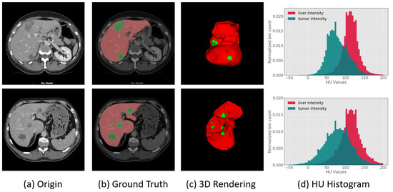
Figure 1. (a) Images of slice of liver and tumor region from CT; (b,c) show two-dimensional and three-dimensional liver and tumor information, respectively, where the red portion represents the normal liver region, and the green portion represents the tumor region; and (d) is the HU values histogram distribution of the liver and tumor from CT, in which the red portion represents the liver, the green portion represents the tumor, and the shaded portion indicates that the HU values of the liver and tumor have a large number of overlapping areas.

These problems prevent the accurate segmentation of medical images. To solve the above problems, we propose a novel cascaded 2.5D FCNs learning framework for the segmentation of the liver and tumor in medical images and design a new boundary loss function for network optimization. The boundary loss function can effectively help the convolutional neural network(CNN) deliberately learn boundary and contour features in medical images. The proposed method can effectively segment medical images and can reduce false-positive cases. Furthermore, the proposed 2.5D FCNs can reduce the cost of VRAM and the utilization of computing resources. Specifically, the contributions of this paper are as follows:

• A boundary loss function is proposed to help capture more boundary and contour features of the liver and tumor, from CT images, and to make the segmentation boundaries smoother;
• A cascading 2.5D FCNs based on the residual network is proposed, which can effectively segment the liver and tumor in CT images and can reduce VRAM cost;
• A post-processing method for the image boundary is presented to reduce false-positive cases, which can further improve segmentation accuracy.

The rest of the paper is organized as follows—related work is reviewed in Section 2. The proposed method is described in detail in Section 3. Details and experimental results are presented in Section 4. In Section 5, a discussion and summary of the proposed method are given.

2. Related Work

In recent years, the segmentation of the liver and tumor has mainly been performed by using some methods of hand-crafted features, such as threshold and region growing. The development of deep learning has achieved excellent results in the computer vision field, including the automatic segmentation of medical images. Since the segmentation of the liver and tumor is chosen as the experimental case, we primarily discuss work related to this topic.

2.1. The Methods Based on Hand-Crafted Features

In early work, researchers have mainly the used threshold method [1], region growing method [2] and methods based on machine learning [3,27,28] for the liver and tumor segmentation. The threshold method mainly determines whether the brightness value in the medical images is greater than a threshold value to determine whether the target pixel belongs to the foreground or the background. However, the threshold method is often not effective for images with many overlapping areas. Different region growing methods are also common in the liver and tumor segmentation tasks. By selecting seed points, the region growing method gradually gathers pixels similar to the seed points into a larger area. For instance, Wong et al. [2] proposed a 2D region growing method to segment tumors empirically. However, the region growing method needs to manually select the seed points and cannot complete the task of automatic segmentation. Machine learning-based approaches have also been used to segment the tumor in medical images. For instance, Vorontsov et al. [3] proposed a method to segment tumors by using a support vector machine (SVM) classifier. Similar to this method, Kuo et al. [28] proposed texture feature vectors to train SVMs and segment the liver and tumor. In addition, Rundo et al. [29] proposed a two-stage computational framework based on unsupervised Fuzzy C-Means Clustering (FCM) techniques that could achieve the automated sub-segmentation of the different dense tissue from CT. This method can be readily integrated into clinical research environments. Le et al. [27] proposed a fast-moving algorithm to generate an initial region and train a separate feedforward network for classifying the tumor. The level set method is also widely used by researchers. The advantages of the numerical calculation of curves and surfaces provide an excellent solution for the segmentation of medical images [30]. For example, Jimenez-Carretero et al. [31] proposed a multiresolution 3D level set method with an adaptive curvature skill to classify tumors. Although there are many excellent traditional methods for the segmentation of the liver and tumor, the disadvantages of relying on hand-crafted features and insufficient segmentation accuracy cause the traditional method to be difficult in the task of automatic liver and tumor segmentation.

2.2. The Methods Based on Deep Learning

In recent years, deep learning methods have achieved great success in many tasks of the computer vision field, such as classification, segmentation and detection [32,33]. For example, the end-to-end convolutional neural network can continuously explore and learn new image feature representations and can classify each pixel in the image to achieve image segmentation. In the early days, the methods of most researchers obtain tissues and organs in medical images by performing patchwise image classification [34]. These segmentation methods, which only consider the local context information, easily fail in challenging modalities, such as MRI, since there are too many misclassified voxels in the image. Patchwise approaches [35] can obtain more accurate segmentation results by constantly putting forward the proposed region input into CNN. However, many calculations are redundant when dealing with patched extracted intensively by CNNs; therefore, their total running time is too long [36]. Based on the emergence of end-to-end convolutional neural networks, more image feature representations can be continuously explored. For instance, each pixel in the image can be classified to achieve the goal of automatic image segmentation [7].

Considering the excellent effect of deep convolutional neural networks, many researchers have designed various networks to segment the liver and tumor by using the strong learning ability of convolutional neural networks. For instance, Many researchers have combined conditional random fields (CRFs) with deep learning techniques and applied them in medical image segmentation. 3D CRFs is a conditional probability distribution model for a given set of input sequences and another set of output sequences. As each voxel i in 3D data has a corresponding category $y_i$, each pixel is taken as a node and the relationship between pixels is taken as an edge to form a conditional random field. It can be used as a post-processing method to enhance deep learning. The essence of CRFs is to predict its true category $y_i$ by observing the probability $x_i$ of voxel i. Christ et al. [9,37] designed cascaded FCNs for the segmentation of the liver and tumor and used 3D (CRFs) for postprocessing. Zormpas-Petridis et al. [38] proposed a novel superpixel-based conditional random fields (SuperCRF) that could improve the classification of the cells by incorporating global and local context for enhanced deep learning. CRFs can also integrate into deep learning as a network module. In [39], Zheng et al. formulated CRFs with Gaussian pairwise potentials and mean-field approximate inference as RNNs. Then they plugged the RNNs into CNN and applied this method to the problem of semantic image segmentation, obtaining top results on the VOC dataset. Lapa et al. [40] also incorporated CRFs into an end-to-end network for medical image segmentation. In addition, many deep learning methods to enhance feature expression have also been proposed for medical image segmentation. For example, Singh et al. [41] proposed a receptive-field-aware (RFA) module that can enlarge the receptive field of the segmentation models and increase the learning ability of the model without information loss. Chen et al. [42] proposed an encoding and decoding neural network to segment tumors, which used the attention network to mixture the high and low-level image features and improve the segmentation accuracy. The structure and dimension of networks also play an important role in medical image segmentation. Milletari et al. [43] proposed an end-to-end 3D fully convolutional network for lesion segmentation in prostate CT data, which can fully explore the 3D context information and use the similarity coefficient to optimize the network during training. Li et al. [18] proposed a 2D and 3D hybrid dense network to segment the liver and tumor. Zhu et al. [15] designed a 2.5D recursive neural network for tumor segmentation, which used a continuous prostate biopsy as a sequence of data to explore the context information, which assisted in the division. Yun et al. [44] proposed a new 2.5D network for the chest CT segmentation. In this method, three 2D CNNs are trained to separately segment from the sagittal, coronal, and axial planes. Afterwards, the segmentation results from each plane are fused to obtain the final segmentation results. For efficient volumetric medical image segmentation, some studies have also focused on fusing features extracted from 2D and 3D CNNs to obtain higher efficiency. Zhou et al. [45] proposed a hybrid 2.5D method for chronic stroke lesion segmentation, which fuse 2D and 3D convolution in their network and achieves excellent performance.

However, deep learning methods require considerable time and memory resources. Moreover, the segmentation targets of medical images often have apparent contour shapes and fuzzy boundary features, and many deep learning methods have not specifically explored the boundary features. To utilize the boundary information, in this paper, we present a boundary loss function for the proposed 2.5D FCNs, which not only solve the problem of insufficient boundary feature exploration but also reduce the cost of computing resources.

2.3. The Loss Function for Networks Optimization

During the process of neural network training, the loss functions play an essential role in optimizing network parameters. Researchers can obtain higher segmentation accuracy by selecting the appropriate loss functions to optimize the network model. According to the derivation of the loss function [46], they can be divided into four categories: distribution-based loss, region-based loss, boundary-based loss and compound loss. Cross-entropy is a common distribution-based loss and it optimized the networks by minimizing dissimilarity between two distributions. Focal loss [47] is derived from cross-entropy. Lin et al. proposed the focal loss for target scene detection, which can effectively solve the imbalance between foreground and background in the training process. However, the focal loss function is very sensitive to relevant parameters, and it requires repeated adjustment to find an appropriate value. Dice loss is a region-based loss and it can optimize the networks by minimizing the mismatch. In essence, Tversky loss [48] is a generalization of the Dice loss, which can achieve an improved tradeoff between precision and recall by weighting the relevant parameters. Hausdorff distance loss [49] a boundary-based loss and aims to minimize the distance between ground truth and predicted segmentation. Compound loss is the (weighted) combination between the above loss functions, such as the combination of Dice loss and cross-entropy loss [50].

To better describe the proposed boundary loss function, we first briefly introduce the other three loss functions used in this paper—the cross-entropy loss function [19], similarity coefficient loss function [18,43] and contour loss function [21]. They are all representative loss functions in medical image segmentation. In the following expressions, the marked image and the predicted image are represented as T, $P\in {[0,1]}^{w\times h}$, where 0 and 1 represent the pixels in the background and foreground, respectively; w and h represent the width and height of the image, respectively; n represents the index of pixel space of the image; and N is the pixel space of the image. $T_n$ and $P_n$ represent the value of 0 or 1 at the position index n, respectively.

Cross-entropy loss Cross-entropy is an important concept in Shannon information theory. Cross-entropy is used to measure the difference between two probability distributions. Cross-entropy can be used as a loss function in deep learning networks. The cross-entropy loss function is a widely used pixel-level metric [19,20] to evaluate classification or segmentation model performance. For the sake of description, let us take a binary problem as an example, then, the binary cross-entropy loss function $L_b$ can be expressed as follows:

$$L_b(T,P)=-\frac{1}{N}\sum _{n=1}^N[T_n\times log\left(P_n\right)+(1-T_n)\times log(1-P_n)].$$

(1)

Cross-entropy is sufficient to address most segmentation problems. However, in the case of category imbalance, it is necessary to choose the category weight reasonably well to achieve effective segmentation results.

Dice loss Dice coefficient is a set similarity measurement function, which is usually used to calculate the similarity of two samples. The similarity coefficient can be a common index to evaluate the segmentation performance. Milletari et al. [43] and Li et al. [18] demonstrated that the similarity coefficient could also be used as a useful loss function. The similarity coefficient measures the overlap rate between the labelled image and the predicted image. Its range is [0, 1], where 1 represents complete overlapping, 0 represents no overlapping, and other values represent partial overlapping. The similarity coefficient d can be expressed as follows:

$$d(T,P)=2\times \frac{{\sum }_{n=1}^N(T_n\times P_n)}{{\sum }_{n=1}^N(T_n+P_n)}.$$

(2)

The loss of the similarity coefficient $L_d$ is expressed as follows:

$$L_d(T,P)=1-d(T,P).$$

(3)

The loss of similarity coefficient loss function can solve the segmentation problem of extremely unbalanced categories. However, it neglects the feature of the contour structure in the segmentation target.

Contour loss Chen et al. [21] integrated the area and scale information as a loss function with contour information, representing the image learning features with specific contours. The contour loss function $L_a$ is expressed as follows:

$$L_a=l+\lambda \times r,$$

(4)

where l is the length of the contour; and $\lambda$ is the weight of the area r. Unlike the similarity coefficient loss function, the contour loss function considers the segmentation target’s contour attribute and obtains an improved segmentation effect. However, the contour loss function effect is not sufficient for the target boundary fuzzy data.

3. Method

The two 2.5D FCNs used in this paper are based on the idea of a cascading segmentation method. Each of the cascading 2.5D FCNs undergoes preliminary training under the combined loss function and boundary loss function, improving segmentation accuracy and optimizing network parameters. In addition, we integrate the post-processing method into our segmentation framework to further improve the segmentation effect. The flow of the proposed method is described in Figure 2.

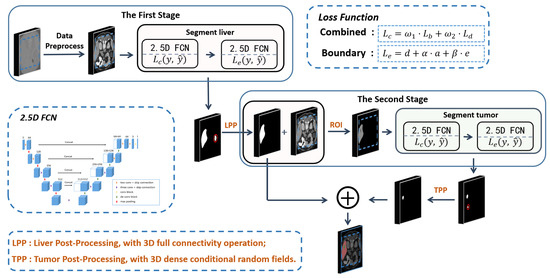
Figure 2. The flow chart of the proposed method. The whole process is divided into two stages. The first stage is to segment liver shape from the image, and the second stage is to extract tumor shape based on the results from the first stage. In the first stage, the ROI of the liver in the image is extracted with a residual network to improve the accuracy of the 2.5D FCN for liver segmentation. Then, a 2.5D FCN is proposed to segment the liver in the ROI. In the second stage, the tumor is segmented with the same 2.5D FCN. each 2.5D FCN is first trained with the combined loss function $L_c$ in Formula (7), and the boundary loss function $L_e$ in Formula (8). Finally, LPP and TPP are performed on the liver and tumor segmentation results, respectively, by merging liver and tumor results as the final output.

3.1. Image Preprocessing

The density value of the CT data, that is, HU, is distributed within [−1024, 2048], which spans an extensive range [38]. To reduce the influence of other tissues and organs in CT during network training, we perform different preprocessing operations for liver and tumor segmentation. The liver and tumor density values are mostly distributed within [−150, 300] through statistics. Therefore, we truncate the image density value of all CT scans within [−150, 300] and normalize the data to [0, 1], as shown in Figure 3. To segment the tumor, we truncate the image density values of all CT scans to [−135, 265]. Since the tumor’s pixel values are lower than the liver image, and the HU value is mostly distributed within [−135, 265]. To highlight the tumor area, we do not directly normalize the data to [0, 1]. Instead, we first scale the data to [0, 255] after adjusting the HU value. Then, we reverse the grey and scale the data to [0, 1] to accelerate the convergence speed of the network.

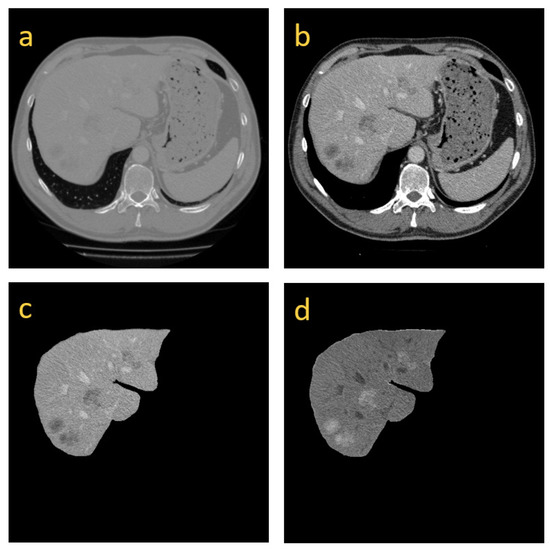
Figure 3. (a) is the original image; (b) is the resulting image after we truncate HUs within [−150, 300]; (c) is the preprocessing image for the segmentation of the tumor, whose HUs are within [−135, 265]; and (d) is the image in which the gray values are reversed from (c).

3.2. Model Structure

Many studies have shown that the symmetric network of encoding and decoding is helpful to improve segmentation performance [13,14,20]. In this paper, the proposed model is similar to a 3D U-shaped full convolutional neural network proposed by Milletari et al. [43]. However, unlike their model, we design a 2.5D network to reduce the need for training parameters and VRAM occupancy. The 2.5D network is realized by inputting five adjacent slices to ensure that the occupation of VARM is reduced and that the exploration of 3D data spatial information is improved. In addition, the basic blocks of the proposed network are built by using the residual structure [6]. Each basic block based on the residual structure consists of two or three convolutional layers and a shortcut connection. The residual structure can avoid network degradation while training a deeper network and exploring more features to improve the model’s performance. The residual structure is expressed as follows:

$$x_{l+1}=x_l+F(x_l,w_l),$$

(5)

where $x_l$ is the input in the l layer of the network, $x_{l+1}$ is its output, $F(·)$ is the residual function, and $w_l$ is the weight parameter of the corresponding residual block.

Based on the basic block, that is, the residual structure, a 2.5D FCN network is designed, as shown in Figure 4. A common 2D network inputs an image and outputs a corresponding probabilistic map. Unlike normal 2D models, the input for our model consists of five cascading slices. The model outputs a segmentation feature map, which corresponds to the middle slice of the five slices. The descriptive formula of the structure of the full convolutional neural network is described as follows:

$$\mathit{I}=f_{2.5D}(\mathit{X},\widehat{L},{\theta }^{{}^{\prime }}),$$

(6)

where $f_{2.5D}$ is the formula of the 2.5D full convolutional network and $\mathit{X}$ represents five cascaded slices, which are input into the full convolutional network. ${\theta }^{{}^{\prime }}$ describes the parameters that are used to train the network; $\widehat{L}$ is the corresponding loss function optimization; and I is the output result of the network $f_{2.5D}$. Therefore, a larger image content on the x-y plane and z-axis context information is provided. Compared with 3D networks, our network model not only maintains larger input image content but also add deeper layers to the networks. As described in Figure 4, two convolution blocks with the residual structure are used to structure the first two layers inside the model’s left part. The last three layers inside the left part of the model are structured by using three other convolution blocks with the residual structure, which can acquire more feature information. All convolution blocks consist of a convolution layer with a $3\times 3$ kernel, a batch normalization layer and a ReLU activation layer. On the right part of the model is a symmetric decoding structure to restore the resolution of the input image and to output segmentation results. Compard with some 2.5D models [44,45], our 2.5D FCN is different in that it incorporates interslice information into 2D CNNs to explore the spatial correlation. Specifically, since our model takes a set of adjacent slices as input and outputs the segmentation result corresponding to the centre slice, which makes it effective in reducing parameters and memory usage.

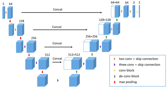
Figure 4. The proposed 2.5D FCN structure is shown in the figure above. The CT slices of $H\times W\times 5$ are fed into the network and the model outputs the probability map of $H\times W\times 1$.

3.3. Boundary Loss Function

In medical images, the area of interest usually has a specific shape and the boundary is often blurred. It is difficult for networks with the cross-entropy loss function or similarity coefficient loss function to learn boundary and contour features. Therefore, we propose a new loss function for effective learning of boundary and contour features.

The boundary loss function can better optimize the network to explore the boundary features, which makes the boundary of the segmentation result smoother. However, to speed up the convergence rate of the network, we first use the combined loss function of cross-entropy and similarity coefficient to optimize the network parameters in each stage of network training. After the network loss decreases to a certain degree, that is, the combined loss can no longer be reduced by changing the learning rate, the boundary loss function is used to optimize the network further. The combined loss function of cross-entropy and similarity coefficient can be described as follows:

$$L_c={\omega }_1\times L_b(T,P)+{\omega }_2\times L_d(T,P),$$

(7)

where ${\omega }_1$ and ${\omega }_2$ are the corresponding weights of the loss function of the cross-entropy and similarity coefficient, respectively. Afterwards, the boundary loss function is used to optimize network parameters to better learn the boundary information in the image. The boundary loss function $L_e$ can be described as follows:

$$L_e=d+\alpha \times a+\beta \times e,$$

(8)

where d, a and e indicate the distance, area and boundary, respectively, and there is little difference in detail with l and r in Formula (4). $\alpha$ and $\beta$ are the weights of the area and the boundary, respectively. d, a and e can be written in pixelwise manner as follows:

$$d=\sum _{i=1,j=1}^N\sqrt{{(\Delta u_{x_{i,j}})}^2+{(\Delta u_{y_{i,j}})}^2},$$

(9)

and

$$a=\left|\sum _{i=1,j=1}^N{u}_{i,j}(1-v_{i,j})\right|+\left|\sum _{i=1,j=1}^N{v}_{i,j}(1-u_{i,j})\right|,$$

(10)

where $v_{i,j}$ and $u_{i,j}$ represent the values of the marked and predicted values, respectively. $x_{i,j}$ and $y_{i,j}$ are two coordinate values of pixel $(i,j)$. N is the pixel space. $\Delta u$ represents the result from subtracting the value of the corresponding pixel index.

We assume that the image with the true value is designated as A. B is the resulting image of four iterative expansions of A. C is the resulting image of four iterative corrosions of A. The extraboundary is $Om=A\otimes B$, and the intraboundary is $Im=A\otimes C$, where ⊗ represents an xor operation. Then, $Im$ and $Om$ are used to obtain the predicted values of extraboundary O and intraboundary I. Thus, the boundary e can be described as follows:

$$e=\left|\sum _{i=1,j=1}^N{O}_{i,j}+\sum _{i=1,j=1}^N(1-I_{i,j})\right|.$$

(11)

The boundary loss function considers the distance, area and boundary as contour features simultaneously. For distance, Formula (9), the adjacent pixel points in the same target tissue and organ area in medical images have a certain similarity; therefore, taking distance as part of the loss function, namely, minimizing the difference between adjacent pixel points, can achieve the purpose of optimizing network parameters. For area, when using Formula (10), similar to the Dice loss function, it is essential to maximize the pixel value in the target area and minimize the pixel value in the background to ensure effective segmentation. For the boundary, Formula (11), the boundary between organs in the medical image is, therefore, the boundary can be weighted. The boundary can be taken as a part of the loss function to optimize the segmentation of the target boundary and to make it smoother. If the segmentation boundary of the target is distinct, the weighted constraint of e in the loss function is strong. If segmentation does not need boundary information, the total loss degenerates into Dice loss, that is, losing its utility in optimizing edge segmentation.

3.4. Training and Testing

In the training phase, we preprocess the data to train the first 2.5D FCN for segmenting the liver. To accelerate the convergence of the network, the combined loss function of Formula (7) is used to preliminarily the network during the training. Afterwards, the boundary loss function is used to train the network further to improve the segmentation performance. For segmenting the tumor, the liver mask is red dilated iteratively five times for the network to focus more on the tumor during the training process, that is, the liver mask is dilated five pixels. Afterwards, the dilated mask is used to obtain the ROI from the CT data. The corresponding data processing is performed to train the second 2.5D FCN for segmenting the tumor. The loss optimization method during training is the same as that in the segmenting liver stage.

In the test phase, we use the first 2.5D FCN to obtain the liver segmentation results after data preprocessing. Afterwards, we perform post-processing on the probability map results from the network output and save the liver segmentation results. The results of the liver segmentation are dilated iteratively five times and used as a mask to obtain liver ROIs. In addition, the liver ROI data are processed accordingly. Then, tumor prediction is performed in the ROI. Finally, the tumor probability map output from our network is post-processed. The post-processed results are combined with the liver segmentation results obtained during the first stage as the output of the final segmentation results, and a more accurate segmentation mask of the liver and tumor are obtained.

3.5. Image Post-Processing

After obtaining the segmented liver probability map from the 2.5D FCN, we use the 3D full connectivity operation to reserve the maximum segmentation volume. Then we dilate each slice once as the final segmentation result. For the tumor maps obtained from the 2.5D FCN, we apply 3D dense conditional random fields (CRFs) [51] to them and exclude false-positive cases and false-negative cases with higher than average HU to further improve the accuracy. Finally, we combine the liver results with the results of the tumor as the final output. As shown in Figure 5, after post-processing, the dice and accuracy of the liver increased by $5.1\%$ and $0.7\%$, respectively. In addition, false-positive cases also decreased by $0.7\%$. For the segmentation of the tumor, the dice and accuracy of the tumor increased by $4.1\%$ and $0.7\%$, respectively. In addition, false-positive cases are also decreased by $0.1\%$. The post-processed method can effectively improve segmentation accuracy.

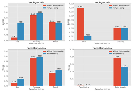
Figure 5. In the segmentation of the liver and tumor, the post-processing method can effectively improve the dice, accuracy and recall, and can reduce the presence of false-positive and false-negative cases.

4. Experiments and Results

4.1. Experimental Environment

We use the 3DIRCADb dataset and the LiTS dataset to train and test our model. The LiTS dataset consists of 131 training CT data and 70 testing CT data. The dataset was obtained from six different clinical sites by using different scanners and protocols. Additionally, the resolution of each data point is very different, among which the resolution of the inter-slice is between 0.55 mm and 1.0 mm, and the resolution of the intraslice is between 0.45 mm and 6.0 mm. For the LiTS dataset, we use 130 data points as training data and 70 data points as test data. The 3DIRCADb dataset contains 20 intravenous enhanced CT scans, 15 of which include tumors. For the 3DIRCADb dataset, of which five of the 20 datasets did not contain tumors, we divided the data into different groups for the segmentation of the liver and tumor. For 3DIRCADb liver segmentation, we use 15 data points as the training set and five data points as the test set, and cross-validation is performed concurrently. For the segmentation of 3DIRCADB tumors, we use 12 data points as the training set and 3 data points as the test set to test our method, and cross-validation is performed.

According to the 2017 LiTS challenge’s evaluation criteria, the Dice Per Case and Dice Global Score are used to evaluate the segmentation performance of the liver and tumor. Dice Per Case is the average value of each CT Dice Score, and Dice Global is used to combine all CT data into one data evaluation Dice Score. In addition, measures of standard volumetric overlap error (VOE), root-mean-square error (RSME), relative voxel difference (RVD), mean symmetric surface distance (ASD), intersection over union (IoU) are also used to assess the performance of liver segmentation.

Our model is trained and tested on a machine with three NVIDIA Tesla K80 graphic processing units (GPUs). We set the initial learning rate to 0.001 in training each 2.5D FCN. The parameter ${\omega }_1,{\omega }_2$ of the combined loss function, that is, Formula (7), is set to 1 for network optimization. For the boundary loss function’s optimization, we set the initial learning rate to 0.00005, and $\alpha$ and $\beta$ are set to 5 and 1, respectively. As shown in Figure 6, $\beta$ can affect the convergence degree of the boundary loss function, although overall, the boundary loss can always approach a similar value. When the $\beta$ value is set to 1, the boundary loss can converge to the lowest point. In addition, we set a training accuracy threshold of 0.002. Whenever the training accuracy is no longer improved beyond the threshold, we multiply the learning rate by a factor of 0.5 to attenuate the learning rate. The entire model is implemented by using Python and Pytorch. During the training, we use data scaling of 0.8∼1.2 times to prevent overfitting. In the test, the total data prediction time is between the 30 s and 100 s, which depends on the number of slices.

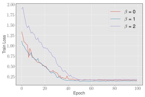
Figure 6. The abscissa represents the number of training iterations, and the ordinate represents the corresponding loss value, Setting different $\beta$ values can slightly affect the convergence degree of the boundary loss function, but the boundary loss can always converge to a similar value on the total. When the $\beta$ value is set to 1, the loss can converge to the lowest point.

4.2. Ablation Study on the LiTS Dataset

To demonstrate the validity of the proposed model and loss, we designed an ablation study to discuss the effects of different configurations of loss and possible models. Specifically, in order to prove the validity of the 2.5D model, we modify the convolution block of the input of the proposed 2.5D model and obtain a 2D model. The 2D model is also a fully convolutional network. Different from the 2.5D network, the input feature dimension of the 2D FCN is modified as $1\times 320\times 320$. Then, we use combined loss, contour loss and boundary loss to optimize the 2D FCN and 2.5D FCN on LiTS dataset, respectively and the results are shown in Table 1. When boundary loss is used to optimize 2D FCN for the segmentation of tumors, 2D FCN yield Dice Per Case and IoU scores of $73.7\%$ and $58.3\%$, respectively. At the same time, the 2.5 FCN with boundary loss yield clear improvements of $0.9\%$ and $1.1\%$ in the Dice Per Case and IoU scores respectively, when compared to the 2D FCN with boundary loss. In addition, 2D FCN yield respectively Dice Per Case and IoU scores of $93.9\%$ and $88.5\%$ for the segmentation of liver. The 2.5 FCN with boundary loss yield clear improvements of $0.4\%$ and $0.8\%$ in the Dice Per Case and IoU scores respectively, when compared to the 2D FCN with boundary loss. Since the spatial dependent information between slices is considered in the input of 2.5D FCN and more spatial feature information can be explored in the subsequent feature exploration. So the 2.5D FCN can effectively improve the segmentation effect of 3D medical images.

Table 1. Performance of different configurations of the proposed method on the LiTS dataset (Dice and IoU: %).

Loss	Tumor		Liver
	Dice Per Case	IoU	Dice Per Case	IoU
2D FCN + Combined loss	65.2	48.4	91.3	84.0
2D FCN + Contour loss	72.4	56.8	93.2	87.3
2D FCN + Boundary loss	73.6	58.3	93.9	88.5
2.5D FCN + Combined loss	68.2	51.8	92.6	86.3
2.5D FCN + Contour loss	73.8	58.5	94.1	88.9
2.5D FCN + Boundary loss	$\mathit{74.5}$	$\mathit{59.4}$	$\mathit{94.3}$	$\mathit{89.3}$

4.3. Loss Analysis on the LiTS Dataset

To verify the effectiveness of the boundary loss function, we use different loss functions to optimize our 2.5D FCN and to test the effect on the LiTS dataset. As shown in Table 2, in the segmentation of the liver, the Dice Global with the cross-entropy, dice and combined loss function is not very different. However, the Dice Global with contour and boundary loss functions achieves excellent results. The Dice Global with proposed the loss is $96.1\%$, which surpasses the other loss functions. In the segmentation of the tumor, the Dice Per Case with a dice loss function is approximately $3.3\%$ higher than that with a cross-entropy loss function. Compared with the loss of cross-entropy and dice, the combined loss function can be improved by at least $2.5\%$ for tumor segmentation, as shown in Figure 7. The above results indicate that the combined loss function is superior to the similarity coefficient loss function or cross-entropy loss function alone. In addition, further optimization with the contour loss function and the boundary loss function after using the combined loss function in the experiment can improve the accuracy to $5.6\%$ and $6.3\%$, respectively. The proposed boundary loss function can optimize the boundary to a certain extent, as shown in Figure 8, to remove false-positive cases more effectively for the subsequent post-processing method. Therefore, our method can obtain higher segmentation accuracy and the Dice Per Case with the proposed loss function is $74.5\%$, which is the highest value among loss functions that are compared.

Table 2. Performance of different loss functions on the LiTS dataset (Dice: %).

Loss	Tumor		Liver
	Dice Per Case	Dice Global	Dice Per Case	Dice Global
Cross-entropy loss	62.4	67.7	91.2	92.6
Dice loss	65.7	68.3	92.3	93.4
Combined loss	68.2	71.2	92.6	93.8
Contour loss	73.8	75.6	94.1	95.2
Boundary loss	$\mathit{74.5}$	$\mathit{77.2}$	$\mathit{94.3}$	$\mathit{96.1}$

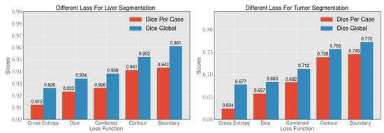
Figure 7. By comparing the cross-entropy loss function, dice loss function, combined loss function, contour loss function and boundary loss function, 2.5D FCNs have an improved segmentation effect when the boundary loss function is used. The boundary loss function can better optimize the segmentation of the boundary of the liver and tumor. Afterwards, the corresponding post-processing method can achieve an excellent segmentation effect.

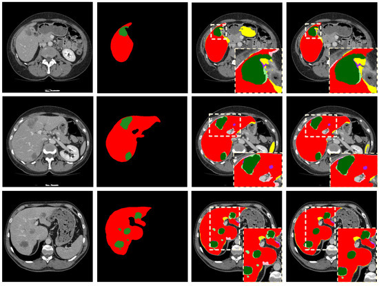
Figure 8. The first column on the left side is the original image; the second column is the corresponding GroundTruth; the third column is the segmentation result using the combined loss function; and the fourth column is the segmentation results using the boundary loss function. In the third and fourth columns, the colors used to represent the segmentation results are as follows: liver TP (red), liver FP (yellow), liver FN (pink), tumor TP (green), tumor FP (purple), tumor FN (light green), liver and tumor TN (black).

4.4. Methods Analysis on the 3DIRCADb Dataset

To verify the robustness of our method, we perform cross-validation based on the 3DIRCADb dataset. The test results are described in Table 3 and Table 4. For liver segmentation, the proposed method is compared with UNet [16] and 2D FCN [9]. 2D UNet is a classical medical image segmentation network, but its model is not deep enough and cannot effectively explore the spatial information in the 3D data due to the limitation of the convolution dimension. Therefore, as shown in Table 3, our method achieves better segmentation accuracy than 2D UNet, and the Dice Global of our method achieves $96.1\%$. As shown in Table 4, compared with 3D H-DenseUNet [18] and 2.5D ResNet [14], the Dice Per Case of our method achieves $68\%$ segmentation of the tumor. Compared with Li et al. [52], the dice of the liver is improved to $96.1\%$ with our method.

Table 3. Comparison of liver segmentation results on the 3DIRCADb dataset.

Model	VOE	RVD	ASD	RSMS	Dice
2D UNet [16]	14.2 ± 5.7	−0.05 ± 0.1	4.3 ± 3.3	8.3 ± 7.5	0.923 ± 0.03
2D FCN [9]	10.7	−1.4	1.5	24.0	0.943
Han et al. [14]	11.6 ± 4.1	−0.03 ± 0.06	3.9 ± 3.9	8.1 ± 9.6	0.938 ± 0.02
Li et al. [53]	$\mathit{9.2}$	−11.2	$\mathit{1.6}$	28.2 -
Li et al. [52]	-	-	-	-	0.945
our method	8.5 ± 6.6	$\mathit{0.01}\pm \mathit{0.02}$	1.6 ± 2.0	$\mathit{3.9}\pm \mathit{6.5}$	$\mathit{0.961}\pm \mathit{0.08}$

Table 4. Comparison of tumor segmentation results on the 3DIRCADb dataset.

Model	VOE	RVD	ASD	RSMS	Dice
2D UNet [16]	62.5 ± 22.3	0.38 ± 1.95	11.1 ± 12.0	16.7 ± 13.8	0.51 ± 0.25
2D FCN [9]	-	-	-	-	0.56 ± 0.26
Han et al. [14]	56.4 ± 13.6	−0.41 ± 0.21	6.3 ± 3.7	$\mathit{11.6}\pm \mathit{7.6}$	0.60 ± 0.12
Li et al. [18]	$\mathit{49.7}\pm \mathit{5.2}$	−0.33 ± 0.10	5.29 ± 6.1	11.1 ± 29.1	0.65 ± 0.02
our method	57.5 ± 13.8	$-\mathit{0.18}\pm \mathit{0.12}$	$\mathit{4.8}\pm \mathit{3.7}$	15.9 ± 12.3	$\mathit{0.68}\pm \mathit{0.15}$

4.5. Methods Analysis on the LiTS Dataset

To further validate our approach, we also train and test on the LiTS dataset and compare our method with some networks, that is, UNet [16], Christ’s network [9], and Chlebus’s network [17], as shown in Table 5. Since these networks all use 2D networks and ignore 3D spatial information, the segmentation accuracy is generally not high. The dice scores of the liver segmentation in our method achieve $96.1\%$ and the result far exceed those 2D methods. The 3D VNet is essentially a 3D UNet-like model. Compared with 3D VNet, the proposed method is $2.2\%$ higher in Dice Global. Yuan et al. [54] and H-DenseUNet [18] have both used 3D network structures. Their methods have a deeper level of networking with 3D networking structures. Therefore, both Dice Per Case and Dice Global in their methods are higher than the 2D network methods. However, the large number of parameters and the utilization of computing resources are fatal disadvantages in these methods. As shown in Table 5, compared with H-DenseUNet [18], our method obtains a performance improvement of $2\%$ of Dice Per Case for the tumor segmentation. Although our liver segmentation score is not higher than those from H-DenseUNet and Yuan’s method, both are 3D networks, our method requires fewer resources. H-DenseNet with a batch size of 1, the resolution of the input image is $5\times 320\times 320$ with our method. The H-DenseNet inputs the image with a resolution of $12\times 224\times 224$, that is, 24 GB VRAM, but our method only uses 4 GB VRAM.

Table 5. Comparison of liver and tumor segmentation results on the LiTS dataset (Dice: %).

Loss	Tumor		Liver
	Dice Per Case	Dice Global	Dice Per Case	Dice Global
2D UNet [16]	65.0	-	-	-
2D FCN [9]	67.0	-	-	-
3D V-Net [43]	-	-	-	93.9
Chlebus et al. [17]	0.680	0.796	-	-
Yuan et al. [54]	65.7	82.0	$\mathit{96.3}$	$\mathit{96.7}$
3D H-DenseUNet [18]	72.2	82.4	96.1	96.5
3D AH-Net [55]	63.4	$\mathit{83.4}$	-	-
Med3D [56]	-	-	-	94.6
3D-DenseUNet [57]	69.6	80.7	96.2	96.7
Wang et al. [58]	-	70.2	-	95.1
our method	$\mathit{74.5}$	77.2	94.3	96.1

5. Conclusions

In this paper, a new cascaded 2.5D FCNs learning framework based on the boundary loss function is proposed to segment the liver and tumor of 3D medical images. Specifically, we integrate distance, area and boundary information as a boundary loss to optimize the parameters of the networks. Boundary loss will force the cascaded 2.5D FCNs to learn more boundary and contour features, so as to improve the segmentation performance of the network. To accurately extract the shapes of the liver and tumor, two types of post-processing for the liver and tumor are adopted for the results with the 2.5D learning framework. Compared with the 2D model and 3D model, the proposed 2.5D network framework can explore sufficient 3D context information while minimizing computing resource requirements. The boundary loss function can optimize the network to learn the features of the boundaries in the observed objects to achieve a smoother segmentation effect for the target boundary.

Although our method can explore specific 3D spatial characteristics, it is still inadequate compared with some 3D models. In addition, the boundary loss function cannot learn the boundary features effectively if the boundary is staggered and too complicated. Therefore, in the future, we will try to plug a dual path attention mechanism module [59] into our model. Dual path attention can incorporate the position and channel feature information and capture more spatial information in the intra-slices and inter-slices of the 3D medical data. At the same time, we will revise the 2.5D network to a lightweight 3D deep learning network. A 3D surface loss based on boundary loss will be implemented and embedded in a lightweight 3D deep learning network. In fact, we have implemented most of the work, but the details of the work are still to be tested for a better segmentation performance.

References

- Soler, L.; Delingette, H.; Malandain, G.; Montagnat, J.; Ayache, N.; Koehl, E.; Dourthe, O.; Malassagne, B.; Smith, M.; Mutter, D.; et al. Fully automatic anatomical, pathological, and functional segmentation from CT scans for hepatic surgery. Comput. Aided Surg. 2001, 6, 131–142. [Google Scholar] [CrossRef] [PubMed]
- Wong, D.; Liu, J.; Yin, F.; Tian, Q.; Xiong, W.; Zhou, J.; Qi, Y.; Han, T.; Venkatesh, S.; Wang, S.-c. A semi-automated method for liver tumor segmentation based on 2D region growing with knowledge-based constraints. In MICCAI Workshop; New York, NY, USA, 2008; Volume 41, p. 159. Available online: https://www.researchgate.net/profile/Sudhakar_Venkatesh/publication/28359603_A_semi-automated_method_for_liver_tumor_segmentation_based_on_2D_region_growing_with/links/02bfe50d078e31a511000000.pdf (accessed on 1 April 2021).
- Vorontsov, E.; Abi-Jaoudeh, N.; Kadoury, S. Metastatic liver tumor segmentation using texture-based omni-directional deformable surface models. In Abdominal Imaging. Computational and Clinical Applications; Springer: Cham, Switzerland, 2014; pp. 74–83. [Google Scholar]
- Havaei, M.; Davy, A.; Warde-Farley, D.; Biard, A.; Courville, A.; Bengio, Y.; Pal, C.; Jodoin, P.M.; Larochelle, H. Brain tumor segmentation with deep neural networks. Med. Image Anal. 2017, 35, 18–31. [Google Scholar] [CrossRef] [PubMed]
- Li, X.; Dou, Q.; Chen, H.; Fu, C.W.; Qi, X.; Belavỳ, D.L.; Armbrecht, G.; Felsenberg, D.; Zheng, G.; Heng, P.A. 3D multi-scale FCN with random modality voxel dropout learning for intervertebral disc localization and segmentation from multi-modality MR images. Med. Image Anal. 2018, 45, 41–54. [Google Scholar] [CrossRef]
- He, K.; Zhang, X.; Ren, S.; Sun, J. Deep residual learning for image recognition. In Proceedings of the IEEE Conference on Computer Vision and Pattern Recognition, Las Vegas, NV, USA, 27–30 June 2016; pp. 770–778. [Google Scholar]
- Long, J.; Shelhamer, E.; Darrell, T. Fully convolutional networks for semantic segmentation. In Proceedings of the 2015 IEEE Conference on Computer Vision and Pattern Recognition (CVPR), Boston, MA, USA, 7–12 June 2015; pp. 3431–3440. [Google Scholar]
- Everingham, M.; Gool, L.; Williams, C.K.; Winn, J.; Zisserman, A. The Pascal Visual Object Classes (VOC) Challenge. Int. J. Comput. Vis. 2009, 88, 303–338. [Google Scholar] [CrossRef]
- Christ, P.; Ettlinger, F.; Grün, F.; Elshaer, M.; Lipková, J.; Schlecht, S.; Ahmaddy, F.; Tatavarty, S.; Bickel, M.; Bilic, P.; et al. Automatic Liver and Tumor Segmentation of CT and MRI Volumes using Cascaded Fully Convolutional Neural Networks. arXiv 2017, arXiv:abs/1702.05970. [Google Scholar]
- Ben-Cohen, A.; Diamant, I.; Klang, E.; Amitai, M.; Greenspan, H. Fully Convolutional Network for Liver Segmentation and Lesions Detection; Springer International Publishing: Berlin/Heidelberg, Germany, 2016. [Google Scholar]
- Zhu, Q.; Du, B.; Wu, J.; Yan, P. A Deep Learning Health Data Analysis Approach: Automatic 3D Prostate MR Segmentation with Densely-Connected Volumetric ConvNets. In Proceedings of the 2018 International Joint Conference on Neural Networks (IJCNN), Rio de Janeiro, Brazil, 8–13 July 2018; pp. 1–6. [Google Scholar]
- Dou, Q.; Chen, H.; Jin, Y.; Yu, L.; Qin, J.; Heng, P.A. 3D deeply supervised network for automatic liver segmentation from CT volumes. In International Conference on Medical Image Computing and Computer-Assisted Intervention; Springer: Berlin/Heidelberg, Germany, 2016; pp. 149–157. [Google Scholar]
- Çiçek, Ö.; Abdulkadir, A.; Lienkamp, S.S.; Brox, T.; Ronneberger, O. 3D U-Net: Learning dense volumetric segmentation from sparse annotation. In International Conference on Medical Image Computing and Computer-Assisted Intervention; Springer: Berlin/Heidelberg, Germany, 2016; pp. 424–432. [Google Scholar]
- Han, X. Automatic liver lesion segmentation using a deep convolutional neural network method. arXiv 2017, arXiv:1704.07239. [Google Scholar]
- Zhu, Q.; Du, B.; Turkbey, B.; Choyke, P.; Yan, P. Exploiting interslice correlation for MRI prostate image segmentation, from recursive neural networks aspect. Complexity 2018, 2018, 4185279. [Google Scholar] [CrossRef]
- Chlebus, G.; Meine, H.; Moltz, J.H.; Schenk, A. Neural network-based automatic liver tumor segmentation with random forest-based candidate filtering. arXiv 2017, arXiv:1706.00842. [Google Scholar]
- Chlebus, G.; Schenk, A.; Moltz, J.H.; van Ginneken, B.; Hahn, H.K.; Meine, H. Automatic liver tumor segmentation in CT with fully convolutional neural networks and object-based postprocessing. Sci. Rep. 2018, 8, 15497. [Google Scholar] [CrossRef]
- Li, X.; Chen, H.; Qi, X.; Dou, Q.; Fu, C.W.; Heng, P.A. H-DenseUNet: Hybrid densely connected UNet for liver and tumor segmentation from CT volumes. IEEE Trans. Med. Imaging 2018, 37, 2663–2674. [Google Scholar] [CrossRef]
- Girshick, R. Fast r-cnn. In Proceedings of the IEEE International Conference on Computer Vision, Santiago, Chile, 7–13 December 2015; pp. 1440–1448. [Google Scholar]
- Ronneberger, O.; Fischer, P.; Brox, T. U-Net: Convolutional Networks for Biomedical Image Segmentation. In International Conference on Medical Image Computing and Computer-Assisted Intervention; Springer: Cham, Switzerland, 2015. [Google Scholar]
- Chen, X.; Williams, B.M.; Vallabhaneni, S.R.; Czanner, G.; Williams, R.; Zheng, Y. Learning active contour models for medical image segmentation. In Proceedings of the IEEE Conference on Computer Vision and Pattern Recognition, Long Beach, CA, USA, 15–20 June 2019; pp. 11632–11640. [Google Scholar]
- Woźniak, M.; Połap, D. Bio-inspired methods modeled for respiratory disease detection from medical images. Swarm Evol. Comput. 2018, 41, 69–96. [Google Scholar] [CrossRef]
- Whitcomb, E.; Choi, W.T.; Jerome, K.; Cook, L.; Landis, C.; Ahn, J.; Te, H.; Esfeh, J.; Hanouneh, I.; Rayhill, S.; et al. Biopsy Specimens From Allograft Liver Contain Histologic Features of Hepatitis C Virus Infection After Virus Eradication. Clin. Gastroenterol. Hepatol. 2017, 15, 1279–1285. [Google Scholar] [CrossRef]
- Ferlay, J.; Shin, H.; Bray, F.; Forman, D.; Mathers, C.; Parkin, D. Estimates of worldwide burden of cancer in 2008: GLOBOCAN 2008. Int. J. Cancer 2010, 127, 2893–2917. [Google Scholar] [CrossRef]
- Bi, L.; Kim, J.; Kumar, A.; Feng, D. Automatic Liver Lesion Detection using Cascaded Deep Residual Networks. arXiv 2017, arXiv:abs/1704.02703. [Google Scholar]
- Almotairi, S.; Kareem, G.; Aouf, M.; Almutairi, B.; Salem, M. Liver Tumor Segmentation in CT Scans Using Modified SegNet. Sensors 2020, 20, 1516. [Google Scholar] [CrossRef] [PubMed]
- Le, T.N.; Huynh, H.T. Liver tumor segmentation from MR images using 3D fast marching algorithm and single hidden layer feedforward neural network. BioMed Res. Int. 2016, 2016, 3219068. [Google Scholar] [CrossRef] [PubMed]
- Kuo, C.L.; Cheng, S.C.; Lin, C.L.; Hsiao, K.F.; Lee, S.H. Texture-based treatment prediction by automatic liver tumor segmentation on computed tomography. In Proceedings of the 2017 International Conference on Computer, Information and Telecommunication Systems (CITS), Dalian, China, 21–23 July 2017; pp. 128–132. [Google Scholar]
- Rundo, L.; Beer, L.; Ursprung, S.; Martín-González, P.; Markowetz, F.; Brenton, J.; Crispin-Ortuzar, M.; Sala, E.; Woitek, R. Tissue-specific and interpretable sub-segmentation of whole tumour burden on CT images by unsupervised fuzzy clustering. Comput. Biol. Med. 2020, 120, 103751. [Google Scholar] [CrossRef]
- Hoogi, A.; Beaulieu, C.F.; Cunha, G.M.; Heba, E.; Sirlin, C.B.; Napel, S.; Rubin, D.L. Adaptive local window for level set segmentation of CT and MRI liver lesions. Med. Image Anal. 2017, 37, 46–55. [Google Scholar] [CrossRef]
- Jimenez-Carretero, D.; Fernandez-De-Manuel, L.; Pascau, J.; Tellado, J.M.; Ramon, E.; Desco, M.; Santos, A.; Ledesma-Carbayo, M.J. Optimal multiresolution 3D level-set method for liver segmentation incorporating local curvature constraints. In Proceedings of the 2011 Annual International Conference of the IEEE Engineering in Medicine and Biology Society, Boston, MA, USA, 30 August–3 September 2011; pp. 3419–3422. [Google Scholar]
- Chen, L.C.; Papandreou, G.; Kokkinos, I.; Murphy, K.; Yuille, A.L. DeepLab: Semantic Image Segmentation with Deep Convolutional Nets, Atrous Convolution, and Fully Connected CRFs. IEEE Trans. Pattern Anal. Mach. Intell. 2018, 40, 834–848. [Google Scholar] [CrossRef]
- Noh, H.; Hong, S.; Han, B. Learning Deconvolution Network for Semantic Segmentation. In Proceedings of the 2015 IEEE International Conference on Computer Vision (ICCV), Santiago, Chile, 7–13 December 2015; pp. 1520–1528. [Google Scholar]
- Kamnitsas, K.; Ledig, C.; Newcombe, V.F.J.; Simpson, J.P.; Kane, A.D.; Menon, D.K.; Rueckert, D.; Glocker, B. Efficient Multi-Scale 3D CNN with Fully Connected CRF for Accurate Brain Lesion Segmentation. Med. Image Anal. 2016, 36, 61. [Google Scholar] [CrossRef]
- He, K.; Georgia, G.; Piotr, D.; Ross, G. Mask R-CNN. In Proceedings of the IEEE International Conference on Computer Vision, Salt Lake City, UT, USA, 18–23 June 2018. [Google Scholar]
- Sermanet, P.; Eigen, D.; Zhang, X.; Mathieu, M.; Fergus, R.; Lecun, Y. OverFeat: Integrated Recognition, Localization and Detection using Convolutional Networks. arXiv 2013, arXiv:1312.6229. [Google Scholar]
- Christ, P.F.; Elshaer, M.E.A.; Ettlinger, F.; Tatavarty, S.; Bickel, M.; Bilic, P.; Rempfler, M.; Armbruster, M.; Hofmann, F.; D’Anastasi, M.; et al. Automatic liver and lesion segmentation in CT using cascaded fully convolutional neural networks and 3D conditional random fields. In International Conference on Medical Image Computing and Computer-Assisted Intervention; Springer: Cham, Switzerland, 2016; pp. 415–423. [Google Scholar]
- Zormpas-Petridis, K.; Failmezger, H.; Raza, S.; Roxanis, I.; Jamin, Y.; Yuan, Y. Superpixel-Based Conditional Random Fields (SuperCRF): Incorporating Global and Local Context for Enhanced Deep Learning in Melanoma Histopathology. Front. Oncol. 2019, 9, 1045. [Google Scholar] [CrossRef]
- Zheng, S.; Jayasumana, S.; Romera-Paredes, B.; Vineet, V.; Su, Z.; Du, D.; Huang, C.; Torr, P. Conditional Random Fields as Recurrent Neural Networks. In Proceedings of the 2015 IEEE International Conference on Computer Vision (ICCV), Santiago, Chile, 7–13 December 2015; pp. 1529–1537. [Google Scholar]
- Lapa, P.; Castelli, M.; Gonçalves, I.; Sala, E.; Rundo, L. A Hybrid End-to-End Approach Integrating Conditional Random Fields into CNNs for Prostate Cancer Detection on MRI. Appl. Sci. 2020, 10, 338. [Google Scholar] [CrossRef]
- Singh, V.K.; Abdel-Nasser, M.; Pandey, N.; Puig, D. LungINFseg: Segmenting COVID-19 Infected Regions in Lung CT Images Based on a Receptive-Field-Aware Deep Learning Framework. Diagnostics 2021, 11, 158. [Google Scholar] [CrossRef]
- Chen, X.; Zhang, R.; Yan, P. Feature fusion encoder decoder network for automatic liver lesion segmentation. In Proceedings of the 2019 IEEE 16th International Symposium on Biomedical Imaging (ISBI 2019), Venice, Italy, 8–11 April 2019; pp. 430–433. [Google Scholar]
- Milletari, F.; Navab, N.; Ahmadi, S.A. V-net: Fully convolutional neural networks for volumetric medical image segmentation. In Proceedings of the 2016 Fourth International Conference on 3D Vision (3DV), Stanford, CA, USA, 25–28 October 2016; pp. 565–571. [Google Scholar]
- Yun, J.; Park, J.; Yu, D.; Yi, J.; Lee, M.; Park, H.J.; Lee, J.; Seo, J.; Kim, N. Improvement of fully automated airway segmentation on volumetric computed tomographic images using a 2.5 dimensional convolutional neural net. Med. Image Anal. 2019, 51, 13–20. [Google Scholar] [CrossRef]
- Zhou, Y.; Huang, W.; Dong, P.; Xia, Y.; Wang, S. D-UNet: A dimension-fusion U shape network for chronic stroke lesion segmentation. IEEE/ACM Trans. Comput. Biol. Bioinform. 2019. [Google Scholar] [CrossRef]
- Ma, J.; Chen, J.; Ng, M.; Huang, R.; Li, Y.; Li, C.; Yang, X.; Martel, A. Loss odyssey in medical image segmentation. Med. Image Anal. 2021, 71, 102035. [Google Scholar] [CrossRef]
- Lin, T.Y.; Goyal, P.; Girshick, R.; He, K.; Dollár, P. Focal Loss for Dense Object Detection. In Proceedings of the IEEE International Conference on Computer Vision, Venice, Italy, 22–29 October 2017. [Google Scholar]
- Salehi, S.; Erdoğmuş, D.; Gholipour, A. Tversky Loss Function for Image Segmentation Using 3D Fully Convolutional Deep Networks. arXiv 2017, arXiv:abs/1706.05721. [Google Scholar]
- Karimi, D.; Salcudean, S.E. Reducing the Hausdorff Distance in Medical Image Segmentation with Convolutional Neural Networks. IEEE Trans. Med Imaging 2020, 39, 499–513. [Google Scholar] [CrossRef] [PubMed]
- Heller, N.; Isensee, F.; Maier-Hein, K.; Hou, X.; Xie, C.; Li, F.; Nan, Y.; Mu, G.; Lin, Z.; Han, M.; et al. The state of the art in kidney and kidney tumor segmentation in contrast-enhanced CT imaging: Results of the KiTS19 Challenge. Med. Image Anal. 2021, 67, 101821. [Google Scholar] [CrossRef] [PubMed]
- Krähenbühl, P.; Koltun, V. Efficient inference in fully connected crfs with gaussian edge potentials. Adv. Neural Inf. Process. Syst. 2011, 24, 109–117. [Google Scholar]
- Li, C.; Wang, X.; Eberl, S.; Fulham, M.; Yin, Y.; Chen, J.; Feng, D.D. A likelihood and local constraint level set model for liver tumor segmentation from CT volumes. IEEE Trans. Biomed. Eng. 2013, 60, 2967–2977. [Google Scholar] [PubMed]
- Li, G.; Chen, X.; Shi, F.; Zhu, W.; Tian, J.; Xiang, D. Automatic liver segmentation based on shape constraints and deformable graph cut in CT images. IEEE Trans. Image Process. 2015, 24, 5315–5329. [Google Scholar] [CrossRef]
- Yuan, Y. Hierarchical convolutional-deconvolutional neural networks for automatic liver and tumor segmentation. arXiv 2017, arXiv:1710.04540. [Google Scholar]
- Liu, S.; Xu, D.; Zhou, S.; Mertelmeier, T.; Wicklein, J.; Jerebko, A.K.; Grbic, S.; Pauly, O.; Cai, T.; Comaniciu, D. 3D Anisotropic Hybrid Network: Transferring Convolutional Features from 2D Images to 3D Anisotropic Volumes. arXiv 2018, arXiv:abs/1711.08580. [Google Scholar]
- Chen, S.; Ma, K.; Zheng, Y. Med3D: Transfer Learning for 3D Medical Image Analysis. arXiv 2019, arXiv:abs/1904.00625. [Google Scholar]
- Alalwan, N.; Abozeid, A.; ElHabshy, A.A.; Alzahrani, A. Efficient 3D Deep Learning Model for Medical Image Semantic Segmentation. Alex. Eng. J. 2020, 60, 1231–1239. [Google Scholar] [CrossRef]
- Wang, L.; Zhang, R.; Chen, Y.; Wang, Y. The application of panoramic segmentation network to medical image segmentation. In Proceedings of the 2020 15th IEEE International Conference on Signal Processing (ICSP), Beijing, China, 6–9 December 2020; Volume 1, pp. 640–645. [Google Scholar]
- Fu, J.; Liu, J.; Tian, H.; Fang, Z.; Lu, H. Dual Attention Network for Scene Segmentation. In Proceedings of the 2019 IEEE/CVF Conference on Computer Vision and Pattern Recognition (CVPR), Long Beach, CA, USA, 16–20 June 2019; pp. 3141–3149. [Google Scholar]
Publisher’s Note: MDPI stays neutral with regard to jurisdictional claims in published maps and institutional affiliations. |
© 2021 by the authors. Licensee MDPI, Basel, Switzerland. This article is an open access article distributed under the terms and conditions of the Creative Commons Attribution (CC BY) license (https://creativecommons.org/licenses/by/4.0/).