Difference-Based Mutation Operation for Neuroevolution of Augmented Topologies ^†

Abstract

In this paper, a novel search operation is proposed for the neuroevolution of augmented topologies, namely the difference-based mutation. This operator uses the differences between individuals in the population to perform more efficient search for optimal weights and structure of the model. The difference is determined according to the innovation numbers assigned to each node and connection, allowing tracking the changes. The implemented neuroevolution algorithm allows backward connections and loops in the topology, and uses a set of mutation operators, including connections merging and deletion. The algorithm is tested on a set of classification problems and the rotary inverted pendulum control problem. The comparison is performed between the basic approach and modified versions. The sensitivity to parameter values is examined. The experimental results prove that the newly developed operator delivers significant improvements to the classification quality in several cases, and allow finding better control algorithms.

1. Introduction

The development of machine learning in recent decades has resulted in several important findings, which allowed artificial neural networks (NN) to become one of the most widely used tools [1]. Today neural networks have found a variety of real-world applications in different spheres. The development of feed-forward, convolutional, recurrent, long short-term memory (LSTM) [2], echo state networks (ESN) [3], and other architectures allowed the basic concept of neural networks to cover a variety of areas where classification, approximation or prediction problems are considered. Despite the popularity of NN, in most cases, the architectures are designed by human experts in the area by hand, and creating new architectures is quite difficult: for example, [4] shows that it is possible to perform the automatic neural architecture search (NAS) to solve the popular CIFAR-10 and ImageNet problems.

There are several approaches to solve the problem of neural architecture search, starting with relatively simple search techniques (adding or removing neurons one by one), up to modern NAS methods. Some of the most popular approaches are based on evolutionary algorithms (EAs), which use the concept of natural evolution to perform a direct search for solutions. Examples of such could be found in [5,6,7], where neural networks are evolved for image classification, showing competitive results compared to hand-designed architectures. Early studies on combining evolutionary algorithms and neural networks have proposed encoding of the architecture to the genetic algorithm (GA) chromosome [8], usually binary, where the maximum number of layers and neurons is limited by the researcher. More recent studies have developed sophisticated schemes and the neuroevolution of augmented topologies (NEAT) [9] is one of them. Unlike other approaches, NEAT allows flexibility in terms of structure, and solves some important problems such as tracking and protecting innovations, as well as low crossover efficiency.

This study is focused on developing new search operators for the NEAT approach, namely the difference-based mutation. This operator allows a more efficient search for optimal weights in the neural network by combining the information stored in different individuals of the population together. The NEAT approach applied in this study is developed to solve classification problems and control problems, and is tested on a set of well-known datasets and one control problem for the rotary inverted pendulum. The main novelty of the contribution is the search operator for parameter optimization, which allows significant improvements of the NEAT algorithm efficiency. This paper is an extended version of the paper presented at the International Workshop on Mathematical Models and Their Applications [10], with sensitivity analysis of scaling factor influence and modified population update scheme.

The rest of the paper is organized as follows: Section 2 contains the main information about the NEAT algorithm used in this study, as well as the specific encoding and mutation operators and describes the proposed mutation operator, Section 3 contains the experimental setup and results, and Section 4 contains the conclusion.

2. Materials and Methods

2.1. Neuroevolution

Searching for better neural architectures stumbles upon the problem of solutions representation. The representation should be designed so that it would allow encoding various types of networks, and an efficient search at the same time. An individual in the developed evolutionary algorithm should contain the encoding of neurons, connections and weights. Some of the early studies on neuroevolution use the scheme, which is often referred to as the Topology and Weight Evolving Artificial Neural Networks (TWEANNs). For example, such methods, described in [11,12], encode the appearance of each node and connection in the phenotype. In [13] the evolutionary algorithm for neural networks training utilized five mutation operators to add or delete nodes and connections, as well as the back-propagation for weights training.

Despite the ability of TWEANNs to perform the search for optimal architectures, they are characterized by a number of significant disadvantages, including the competing conventions problem, described in [9]. The competing conventions problem occurs when the encoding scheme allows several ways of expressing the same solution, i.e., the solution is the same, but the encodings are different. The historical markers, or innovation markers mechanism, proposed in the NEAT approach allows solving the problem of competing conventions.

The original studies on the NEAT algorithm have shown that it could be applied to a variety of problems, including classification, regression, control algorithms, playing games, and so on. In [14] a review of neuro-evolutionary approaches is given, describing the application to various benchmark problems, for example, pole balancing and robot control. Some of the recent studies considered the landscape analysis of the neuroevolutionary approaches [15], other studies investigated applying autocorrelation and measuring ruggedness based on entropy for problem difficulty estimation. Some of the investigations used the hyperheuristic approach to train a NN, which determined the types of operators to be used in the optimization process [16]. In [17] the new loss function is generated using neuroevolution, which allowed improving the training process of classic neural networks.

Although the NEAT algorithm and its modifications have found a wide area of applications, only a few studies have addressed the problem of weight tuning in the trained network. Several studies have tried to solve the problem of weights tuning, for example, in [18] the cooperative coevolution of synapses was proposed, showing significant improvements to the algorithm capabilities. In [19] the cooperative co-evolutionary differential evolution was applied to train ANN weights, however, this approach is not applicable for the case of network topology optimization. In a recent study, [20] the weight tuning for the evolutionary exploration of augmenting memory models, a variation of neuroevolution, is considered. In particular, weights of the same connections in both parents are identified and generated based on an equation, similar to the one used in differential evolution. The results show that the so-called Lamarckian weight inheritance allows providing additional benefit to the selection of weights improves the way the weight search space is traversed. Considering these studies, it can be concluded that the finding suboptimal weight values for evolved architectures represent a significant problem, so that the development of new general weight search operators for neuroevolution is an important research direction, as it would allow improving the performance of many other modifications. In particular, it seems reasonable to transfer the search operators applied in differential evolution, which is a simple yet efficient numerical optimizer.

The next section of this paper contains the description of the encoding scheme used in NEAT, and then the newly developed operators are presented.

2.2. Encoding Scheme Used in NEAT

One of the core concepts of NEAT, which makes it different from many other approaches, is the initialization procedure. NEAT initializes all the structures to be minimal, i.e., only inputs and outputs are connected, and the weights are assigned randomly. All the further search is performed by increasing (augmenting) the structure of the network. This growth is performed by mutation and crossover operators. To encode an individual NEAT uses two sets: a set of nodes and a set of connections, where each element has several properties. An example of encoding in NEAT for a problem with two input variables and one output is shown in Figure 1.

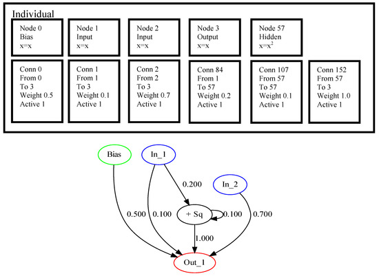
Figure 1. NEAT encoding example.

The upper part of Figure 1 shows the nodes and connections, where numbers are assigned to each of them. The node with number 57 is added after mutation, and it is the 57-th innovation since the beginning of the search process. Here, only the hidden node has some specific operation, while all others perform no transformation on the available data, and in node 57 the input values are squared. The connection genes also have innovation markers, which are assigned during mutation operations. Each connection node keeps the source and destination nodes, marked by innovation numbers, as well as weight coefficient. In addition, the activation flag is set for every connection to allow simple deactivation of them. The three added connections have innovation numbers 84, 107 and 152, and connection 107 makes a loop, i.e., it connects the output from node 57 to itself. The lower part of Figure 1 shows the graphical representation of the encoding as a directed multigraph.

The described encoding scheme, proposed in [9] allows minimal starting for all networks, and thus performs the search in the space of small dimensionality, which is different from TWEANNs or genetic programming (GP), where solutions could be quite complicated even at the first generation. The structure size has no strict limitations in terms of the number of nodes and connections, making NEAT an algorithm with varying chromosome length, which requires specific mutation and crossover. A specific output estimation procedure should be used, for example, in this study the output calculations are repeated until all reachable nodes are activated and the signal is propagated to the outputs. The next section contains the description of mutation and crossover operators used for NEAT in this study.

2.3. Crossover and Mutation Operators Used in NEAT

There were originally two main mutation types proposed for the NEAT algorithm, the first one is adding connections between nodes, and the second is adding nodes in between connections. In this, the set of operators was expanded, and the following mutation types were used:

• Add connection: two nodes are selected randomly, and connected to each user. The weight of the connection is assigned randomly in the following way: first a random value from [0,1] is generated, and if it is smaller then 0.5, then the weight is set as a normal distributed random number with a mean equal to 0 and standard deviation set to 0.1 ($normrand(0,0.1)$). Otherwise, the weight it set close to 1, i.e., $normrand(1,0.1)$. A new innovation number is assigned to the connection.
• Mutating random node: the type of operation performed in a randomly chosen node is changed to another one, and the new innovation number is assigned to the node. Only hidden nodes are mutating.
• Connection removal: if the structure of the network is not minimal, then a randomly chosen connection is deleted. The connections between inputs and outputs are never chosen.
• Connections merging: if the network structure contains at least two connections following the same path, i.e., having the same source and destination, then these nodes are merged together, and the weight value is assigned as the sum of weights. The new connection receives the innovation number of one of the merged.
• Adding a node to connection: one of the connections is randomly selected and divided into two, and a node is placed in between. The new node receives a new innovation number and operation, one of the weights is set to 1, while the other keeps the previous value. The connections receive new innovation numbers.
• Assigning random weights: every connection is mutated with a probability of $1/NumberOfConnections$ the connection receives either weight, chosen from $normrand(0,0.1)$ or $normrand(1,0.1)$. Otherwise, the current value of the weight is used as a mean value to generate new as follows: $w=normrand(w,0.01)$, where w is the current weight value. With probability of $1/NumberOfConnections$ each weight is either activated or deactivated.

Each of the six described mutation operators is applied with certain probabilities, shown in Table 1.

Table 1. Probabilities of mutation operators in NEAT.

Mutation Type	Probability to Use
Add connection	0.1
Mutating random node	0.15
Connection removal	0.15
Connections merging	0.2
Adding node to connection	0.1
Assigning random weights	0.2
No mutation/Proposed approach	0.1

Only one of the mutation operators is used for every individual. If some of the conditions required for mutation are not satisfied, then no mutation is applied to an individual. Some of the mutations may result in an invalid structure of the neural network, i.e., there could be nodes not connected to anything or connections with a non-existing destination. To fix the invalid nodes or connections the purging operation is used, which removes them from the solution.

The crossover in NEAT generates a new topology by combining two individuals. The resulting offspring is further used in the mutation step, described above. To perform the crossover, the innovation numbers are used to determine which nodes and connections are the same for both solutions, in particular, the two parents’ mating genes are aligned, i.e., the parts of the chromosome having the same historical markers. The offspring $s_i$ is composed of the genes, which are randomly chosen from the first or second parent, and the disjoint and excess genes are taken from the parent with higher fitness. The disjoint genes are determined as the genes which exist in one parent, but not the other, while there is still a common part further on in the chromosome. The excess genes are the tail genes of the parent individuals, which are only present in one of them. A more detailed description of the crossover in NEAT could be found in [9].

2.4. The General Scheme of the NEAT Algorithm

The NEAT algorithm follows the main steps of every evolutionary algorithm, such as selection, crossover, mutation, but also uses specific operators, such as speciation. The main steps of NEAT are presented in Algorithm 1.

Algorithm 1 NEAT

1: for $gen=1$ to $NG$ do

2:  Initialize population P with minimal solutions, calculate fitness $fi{t}_i$, $i=1,\dots ,N$

3:  Assign species numbers to every individual

4:  for $i=1$ to N do

5:    Perform tournament-based selection (t = 2) to get index $tr$

6:    Perform crossover between $P_i$ and $P_{tr}$, save offspring to $O_i$

7:    Select the mutation operator to be used

8:    Perform mutation on $O_i$ and calculate fitness

9:   end for

10:  Perform speciation of combined parents P and offspring O populations

11:  Create new population from the representatives of every species

12: end for

13: Return best found solution

In Algorithm 1 the following notations are used: $NG$ is the total number of generations, P is the current population, O is the offspring population, $fit$ is the fitness values array, N is the population size.

The speciation mechanism of NEAT uses historical markings to determine the distance between solutions in the population, allowing to cluster individuals into several groups based on their structural similarity. The distance $\delta$ between two networks is measured as the linear combination of the number of excess (E) and disjoint (D) genes, as well as the average of weights difference ($\overline{W}$) [9]:

$$\delta =c_1\ast E/L_g+c_2\ast D/L_g+c_3\ast \overline{W},$$

(1)

where coefficients $c_1$, $c_2$ and $c_3$ determine the importance of each factor, and $L_g$ is the number of connections genes.

The species in NEAT are numbered in the order of their appearance, and at the beginning, after initialization, the first individual is used as the representative of the first species. Next, all other individuals are tested to be similar to each representative, chosen randomly, using the distance metric. If an individual is close to the representative, i.e., ${\delta }_i$ is less than the threshold value, then this individual is added to the species. If an individual is far from all existing species, it forms a new one and becomes its representative. The median distance between two individuals in the population was used as the threshold value for speciation.

Once the speciation is performed for the joint population of parents and offspring, the fitness sharing mechanism is used to determine how many individuals of each species should be represented in the next generation. The adjusted fitness ${fi{t}_i}^{\prime }$ is calculated based on distance $\delta$ to other individuals:

$$fi{t}_i^{\prime }=\frac{fi{t}_i}{{\sum }_{j=1}^{N}sh\left(\delta \right(i,j\left)\right)},$$

(2)

where $sh\left(\right)$ is the sharing function, set to 1 if $\delta$ is below the threshold, and 0 otherwise. The number of individuals to be taken from each species is calculated as:

$$N_k=\frac{\overline{fi{t}_k}}{\overline{fi{t}_{total}}}N,$$

(3)

where $\overline{fi{t}_k}$ is the average fitness of species k, and $\overline{fi{t}_{total}}$ is the average fitness of the population. First, the species with the best average fitness values are chosen, and the species with small average fitness are removed. The best representative of every species is always copied to the new population. According to [9], the speciation procedure allows protecting innovations, i.e., changes to the individuals which may be destructive currently, but deliver significant improvements later.

In this study the following activation functions were used in the nodes of the network, with x being the sum of all inputs:

• Linear: equals x
• Unsigned step function: equals 1 if $x>0$
• Sine: $sin\left(\pi x\right)$
• Gaussian: $exp(-x\ast x/2)$
• Hyperbolic tangent: $tanh\left(x\right)$
• Sigmoid: $\left(tanh\right(x/2)+1)/2$
• Inverse: $-x$
• Absolute value: $\left|x\right|$
• ReLU: $max(0,x)$
• Cosine: $cos\left(\pi x\right)$
• Squared: $x^2$

The default function is linear (equal), in case the mutation operation generated a new node, one of these activation functions is assigned randomly.

2.5. Proposed Mutation Operation

The NEAT algorithm described above has proved itself to be highly competitive compared to other approaches, and found a variety of applications. However, it could be further improved by introducing new search operators, for example, more efficient crossover and mutation schemes. One of the main problems of NEAT is the lack of an efficient parameter-tuning algorithm. Most of the networks, including fully-connected, convolutional, LSTM and many others use backpropagation algorithm for parameter tuning, however, as long as NEAT generates new structures, often with cycles, applying backpropagation would require an automatic differentiation procedure for every new structure, and in many cases, it would be impossible, as the generated structure could be non-differentiable. Another way of solving this problem could be the application of direct search methods, which do not require derivative calculation. For example, evolutionary algorithms such as genetic algorithm [21], differential evolution [22], or biology-inspired, such as particle swarm optimizer [23] could be applied for weights tuning, as well as many others [24].

However, the existing weights tuning methods have a major disadvantage: they usually tune the weights for one solution, and require quite a lot of computational resources for tuning. In this study, the new difference-based mutation (DBM) scheme is proposed, which does not require additional fitness calculations, and is inspired by the mutation, applied in differential evolution. The proposed difference-based mutation takes into consideration three randomly chosen individuals from the population with indexes $r1$, $r2$ and $r3$, different from each other and the current individual index i, and searches for the corresponding connection genes in them by comparing innovation numbers. The found positions of such numbers are stored in $e_i,e_{r1},e_{r2},e_{r3}$, as long as they could be stored in different parts of the chromosome. The genes which have the same innovation numbers and same weight values are not considered. If at least one innovation number is the same for all four individuals, and the weight values are different, then the mutation is performed to generate new weight values:

$$w_{e_i}=w_{e_{r1}}+F·(w_{e_{r2}}-w_{e_{r3}}),$$

(4)

where F is the scaling factor, and $w_e$ are the weights of corresponding individuals at positions indexed as e. Figure 2 visualizes the identification of the same connections with different weights in DBM.

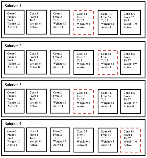
Figure 2. Identifying same genes to perform the difference-based mutation.

The idea behind the difference-based mutation is to use the information stored in the population about every weight coefficient, marked with innovation number, to allow efficient parameter search without additional fitness evaluations. The DBM only changed the weights which are present in several individuals, which means that they are probably important for the network performance.

The proposed DBM approach was used together with other mutation operators described above, and the probability to use it was set to 0.1. Figure 2 shows that, for solutions are required to perform the difference-based mutation. In the example, each of them has the connection node with innovation number 84, and the weight values are different, which makes the DBM possible. Despite the fact there are connections with innovation numbers 0, 1 and 2, they have equal genes in the difference part, which makes DBM for these genes senseless.

Figure 3 shows the result of DBM application to the solutions shown in Figure 2. In Figure 3 the highlighted connections have innovation number 84, and the first solution is considered as current, and the rest three are the randomly chosen ones. The scaling factor F is set to 0.5, so according to Equation (4) the resulting weight equals −0.3.

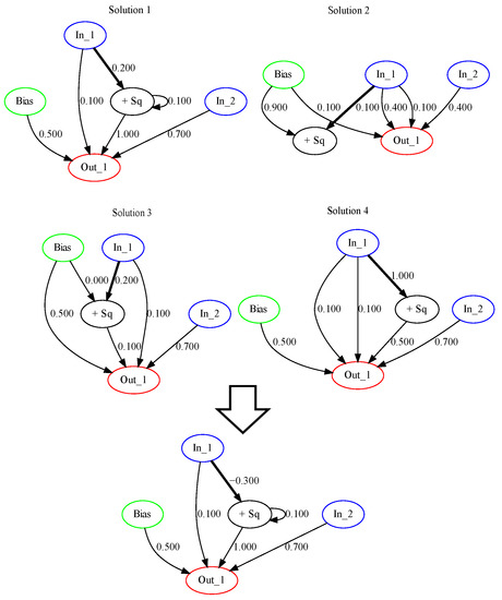
Figure 3. Visualization of DBM example from Figure 2.

In the next section, the experimental setup is described, as well as the algorithm’s parameters and received results.

3. Results

To estimate the efficiency of the proposed approach, two sets of experiments have been performed. First, the classification problems have been considered: in particular, the set of databases from the KEEL repository [25] was used, with the characteristics shown in Table 2. The used datasets are taken from different areas, have a large number of instances or classes, and some of them are imbalanced.

Table 2. Datasets used in the experiments.

Dataset	Number of Instances	Number of Features	Number of Classes
Australian credit	690	14	2
German credit	1000	24	2
Segment	2310	19	7
Phoneme	5404	5	2
Page-blocks	5472	10	5
Twonorm	7400	20	2
Ring	7400	20	2
Magic	19,020	10	2

First, the baseline version of the implemented NEAT algorithm was tested to compare with the modified version with difference-based mutation. The categorical cross-entropy was used as a criterion to be optimized for classification problems. i.e., for an k-class classification problem there were k output nodes, and the softmax layer, used in neural networks [26], was applied. The population size was set to 100 individuals, and the number of generations was set to 500. The maximum number of connections was set to 150, and if this number was exceeded after mutation or crossover, the offspring was eliminated from the next generation. The 10-fold cross-validation was applied to estimate the efficiency of the classifier, which was the accuracy measure, i.e., the number of correctly classified instances relative to total sample size, averaged over 10 folds. The NEAT-DBM was tested with different settings of scaling factor F sampling. In particular, the sampling of F was tested with 5 different mean values used in the normal distribution: $normrand(0.1,0.1), normrand(0.3,0.1), normrand(0.5,0.1),$ $normrand(0.7,0.1),$ $normrand(0.9,0.1)$, i.e., from 0.1 to 0.9 with 0.2 step. This sensitivity analysis was performed to estimate the required F values range for the NEAT algorithm. Figure 4 shows the general scheme of algorithm testing.

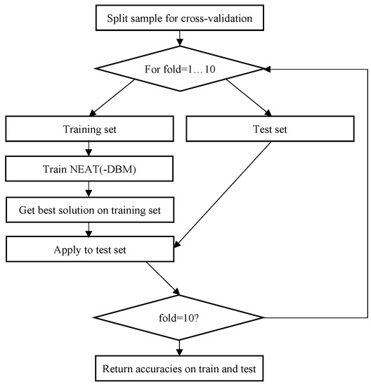
Figure 4. The block scheme of NEAT and NEAT-DBM testing.

Table 3 and Table 4 contain the comparison of NEAT to NEAT-DBM average accuracy with different F sampling on training set.

Table 3. Sensitivity analysis of NEAT-DBM compared to NEAT, training set.

Dataset	$\mathit{NEAT}$	${\mathit{NEAT}}_{\mathit{DBM}0.1}$	${\mathit{NEAT}}_{\mathit{DBM}0.3}$	${\mathit{NEAT}}_{\mathit{DBM}0.5}$	${\mathit{NEAT}}_{\mathit{DBM}0.7}$	${\mathit{NEAT}}_{\mathit{DBM}0.9}$
Australian credit	0.8884	0.8862	0.8857	0.8878	0.8797	0.8886
German credit	0.7900	0.7868	0.7900	0.7882	0.7923	0.7929
Segment	0.7811	0.7973	0.8155	0.8179	0.8220	0.8033
Phoneme	0.8083	0.7914	0.7955	0.7983	0.7954	0.8042
Page-blocks	0.9606	0.9608	0.9620	0.9593	0.9608	0.9609
Twonorm	0.9758	0.9749	0.9755	0.9749	0.9757	0.9767
Ring	0.9026	0.8946	0.8802	0.9020	0.9003	0.9018
Magic	0.8290	0.8350	0.8359	0.8303	0.8391	0.8341

Table 4. Sensitivity analysis of NEAT-DBM compared to NEAT, test set.

Dataset	$\mathit{NEAT}$	${\mathit{NEAT}}_{\mathit{DBM}0.1}$	${\mathit{NEAT}}_{\mathit{DBM}0.3}$	${\mathit{NEAT}}_{\mathit{DBM}0.5}$	${\mathit{NEAT}}_{\mathit{DBM}0.7}$	${\mathit{NEAT}}_{\mathit{DBM}0.9}$
Australian credit	0.8603	0.8647	0.8765	0.8824	0.8971	0.8441
German credit	0.7500	0.7470	0.7480	0.7660	0.7410	0.7420
Segment	0.7874	0.8082	0.8199	0.8087	0.8264	0.7944
Phoneme	0.8074	0.7918	0.7918	0.7950	0.7911	0.8171
Page-blocks	0.9607	0.9653	0.9594	0.9631	0.9603	0.9618
Twonorm	0.9751	0.9758	0.9732	0.9751	0.9739	0.9729
Ring	0.9022	0.8959	0.8733	0.9011	0.9005	0.8992
Magic	0.8271	0.8342	0.8386	0.8305	0.8331	0.8326

The comparison of results in Table 3 and Table 4 shows that applying DBM to NEAT results in improvements for several datasets, for example, Segment dataset on the training sample and Australian credit, Segment, Phoneme on the test set. The best mean values for F sampling are 0.5, 0.7 and 0.9 depending on the problem at hand. In several cases, the performance was smaller than that of the original NEAT, and to check the significance of this difference, the Mann–Whitney statistical tests were performed. Table 5 and Table 6 contain the results of statistical tests, including the test output (1—better, 0—equal, −1—worse) and Z-score.

Table 5. Mann–Whitney statistical tests of NEAT-DBM compared to NEAT, training set.

Dataset	${\mathit{NEAT}}_{\mathit{DBM}0.1}$	${\mathit{NEAT}}_{\mathit{DBM}0.3}$	${\mathit{NEAT}}_{\mathit{DBM}0.5}$	${\mathit{NEAT}}_{\mathit{DBM}0.7}$	${\mathit{NEAT}}_{\mathit{DBM}0.9}$
Australian credit	0, Z = −0.53	0, Z = −0.80	0, Z = −0.42	0, Z = −1.48	0, Z = −0.19
German credit	0, Z = −0.95	0, Z = −0.08	0, Z = −0.72	0, Z = 0.15	0, Z = 0.53
Segment	0, Z = 1.36	1, Z = 2.19	1, Z = 2.42	1, Z = 2.50	0, Z = 1.02
Phoneme	−1, Z = −2.38	0, Z = −1.74	0, Z = −0.72	−1, Z = −2.12	0, Z = −0.98
Page−blocks	0, Z = 0.45	0, Z = 0.79	0, Z = −0.42	0, Z = 0.30	0, Z = 0.61
Twonorm	0, Z = −0.87	0, Z = −1.14	0, Z = −0.68	0, Z = −0.80	0, Z = 1.67
Ring	0, Z = −1.36	0, Z = −1.17	0, Z = 0.08	0, Z = −0.15	0, Z = 0.76
Magic	0, Z = 1.81	0, Z = 1.55	0, Z = 1.13	1, Z = 2.42	0, Z = 1.36

Table 6. Mann–Whitney statistical tests of NEAT-DBM compared to NEAT, test set.

Dataset	${\mathit{NEAT}}_{\mathit{DBM}0.1}$	${\mathit{NEAT}}_{\mathit{DBM}0.3}$	${\mathit{NEAT}}_{\mathit{DBM}0.5}$	${\mathit{NEAT}}_{\mathit{DBM}0.7}$	${\mathit{NEAT}}_{\mathit{DBM}0.9}$
Australian credit	0, Z = −0.04	0, Z = 0.57	0, Z = 0.99	0, Z = 1.68	0, Z = −0.84
German credit	0, Z = −0.61	0, Z = −0.42	0, Z = 1.12	0, Z = −0.89	0, Z = −0.95
Segment	0, Z = 1.03	0, Z = 1.75	0, Z = 1.40	0, Z = 1.93	0, Z = 0.45
Phoneme	0, Z = −1.40	0, Z = −1.33	0, Z = −1.06	0, Z = −1.51	0, Z = 0.76
Page-blocks	0, Z = 1.21	0, Z = −0.27	0, Z = 0.38	0, Z = −0.11	0, Z = 0.19
Twonorm	0, Z = 0.11	0, Z = −0.27	0, Z = 0.00	0, Z = −0.49	0, Z = −0.92
Ring	0, Z = −0.83	0, Z = −1.66	0, Z = −0.04	0, Z = 0.00	0, Z = 0.04
Magic	0, Z = 1.32	1, Z = 2.27	0, Z = 0.83	0, Z = 1.06	0, Z = 1.13

The results in Table 5 and Table 6 show that in most cases the difference was not very significant, although sometimes the Z-score values were close to $1.96$ ($2\sigma$), i.e., threshold value for $p=0.05$ significance level. Nevertheless, for most datasets and scaling factor sampling parameters the Z values are positive, indicating that the NEAT-DBM is, in general, better than standard NEAT.

The ${\mathit{NEAT-DBM}}_{0.5}$ was also compared with alternative approaches, namely the Neural Network, Decision tree [27] and Random forest [28], as well as the K Nearest Neighbors (K-NN) and Support Vector Machines (SVM) and the previously developed Hybrid Evolutionary Fuzzy Classification Algorithm (HEFCA), presented in [29,30]. The Keras library [31] was used to implement a two-layered neural network. The sigmoid is used as an activation function, and the softmax layer was applied at the end. The loss function was implemented as a cross-entropy function, and the adaptive momentum (ADAM) optimizer was applied for weight training. The training of the network on test datasets used the following parameters: the learning rate was set to 0.003, ${\beta }_1$ (exponential decay rate for the first-moment estimates), ${\beta }_2$ (exponential decay rate for the second-moment estimates) were equal to 0.95 and 0.999 respectively, and the learning rate decay was set to 0.005. The first hidden layer contained 100 neurons, and the second hidden layer had 50 neurons. The training was performed for 25 epochs with a batch size of 100. The presented setup is a typical usage scenario for neural networks. In addition to the NN, the Decision Trees (DT) training implemented in sklearn library [32] were used, as well as Random Forest (RF) training, K nearest neighbors classifier (K-NN) and Support Vector Machine for classification (SVM). For these algorithms, the standard training parameters were used for all cases, as this represents a typical usage scenario.

Table 7 contains the comparison on the test set, and Table 8 provides the results of Mann–Whitney statistical test, comparing NEAT-DBM with other approaches.

Table 7. NEAT compared to alternative approaches, test set.

Dataset	HEFCA	NN (Keras)	DT	RF	K-NN	SVM	${\mathbf{NEAT}}_{\mathbf{DBM}0.5}$
Australian credit	0.8537	0.8552	0.8202	0.8724	0.8579	0.8507	0.8824
German credit	0.7280	0.7530	0.6930	0.7610	0.6960	0.7590	0.7660
Segment	0.9100	0.9476	0.9619	0.9801	0.9472	0.8662	0.8087
Phoneme	0.8260	0.7957	0.8760	0.9197	0.8862	0.8442	0.7950
Page-blocks	0.9406	0.9616	0.9613	0.9741	0.9550	0.9055	0.9631
Twonorm	0.9043	0.9792	0.8455	0.9736	0.9728	0.9803	0.9751
Ring	0.9237	0.8262	0.8782	0.9500	0.6888	0.9781	0.9011
Magic	0.8415	0.8274	0.8157	0.8790	0.8072	0.8198	0.8369

Table 8. Mann–Whitney statistical tests of NEAT-DBM compared to alternative approaches, test set.

Dataset	HEFCA	NN (Keras)	DT	RF	K-NN	SVM
Australian credit	0, Z = 0.91	0, Z = 0.98	1, Z = 2.27	0, Z = 0.08	0, Z = 0.76	0, Z = 1.44
German credit	1, Z = 2.56	0, Z = 0.57	1, Z = 2.81	0, Z = 0.04	1, Z = 3.07	0, Z = 0.53
Segment	−1, Z = −3.79	−1, Z = −3.79	−1, Z = −3.80	−1, Z = −3.81	−1, Z = −3.79	−1, Z = −3.56
Phoneme	−1, Z = −2.99	0, Z = 0.00	−1, Z = −3.78	−1, Z = −3.79	−1, Z = −3.79	−1, Z = −3.63
Page−blocks	1, Z = 3.67	0, Z = 0.45	0, Z = 0.30	−1, Z = −3.18	1, Z = 2.35	1, Z = 3.79
Twonorm	1, Z = 3.80	0, Z = −1.44	1, Z = 3.80	0, Z = 0.68	0, Z = 1.14	−1, Z = −2.81
Ring	−1, Z = −3.48	1, Z = 3.78	1, Z = 3.10	−1, Z = −3.78	1, Z = 3.78	−1, Z = −3.78
Magic	0, Z = −1.21	1, Z = 2.19	1, Z = 3.78	−1, Z = −3.78	1, Z = 3.78	1, Z = 3.78

The modified NEAT with DBM was able to get the best test set accuracy for Australian credit, German credit, and ranked second for the Page-blocks and third for the Twonorm datasets. However, it appeared to be worse than all other methods for the Segment dataset, and has similar performance to the NN trained in Keras on the Phoneme dataset, where the rule or tree-based approaches have achieved much better results. This shows that NEAT has certain potential when solving some problems, however, its performance is similar to a feed-forward neural net due to approach similarity. The statistical test in Table 8 shows that NEAT is capable of significantly outperforming decision tree, K-NN, HEFCA, SVM and conventional neural net on several datasets, although when compared to the random forest, it usually shows worse results. The reason for that could be that the RF is an ensemble-based classifier, while all others are single classifiers. Combining several neural nets designed by NEAT-DBM into an ensemble is one of the ways to improve generalization ability.

Figure 5 shows an example of solution trained by NEAT-DBM for the Phoneme dataset.

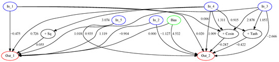
Figure 5. One of the solutions to the Phoneme dataset, test accuracy is 0.80705.

Figure 5 shows that NEAT-DBM is capable of designing relatively compact models with few connections, thus making it possible to solve the classification problems with minimum computational requirements.

For the second set of experiments, the control problem was considered, in particular the stabilizing of the Rotary Inverted Pendulum (RIP). Due to the complexity of this problem and its properties, such as nonlinearity, non-minimum phase and instability, it is often considered as a test problem in the control community. If an algorithm is capable of solving this problem, it should be able to solve many others, such as control of a space booster rocket, automatic aircraft landing system, stabilization of a cabin in a ship, etc. [33]. This was the main reason why this problem was considered in this study.

There are several known problems which include pendulum stabilization. In the RIP problem, the pendulum is mounted on the output arm, which is driven by a servo motor. The position of the pendulum and the arm are measured by encoders. The input to the system is the servo motor voltage and direction. The pendulum has one stable equilibrium point, when the pendulum is pointing down, and another unstable point, where it is pointing up, and the goal is to keep it up and turn the arm to the desired angle. In this study, the model described in [34] is used for experiments. The system is described with the following state variables:

$${\left[x_1{x}_2{x}_3{x}_4\right]}^T={\left[{\theta }_1{\theta }_2{\theta }_1^{\prime }{\theta }_2^{\prime }\right]}^T$$

(5)

These four state variables are the input signal for the controller. Figure 6 shows the RIP and its main characteristics. The full list of parameters and their values was taken from [34] and is provided in Table 9. The modeling was performed with step size of h = 0.01 and time Tmax = 10 s. During modeling, the number of revolutions of arm and pendulum was also measured.

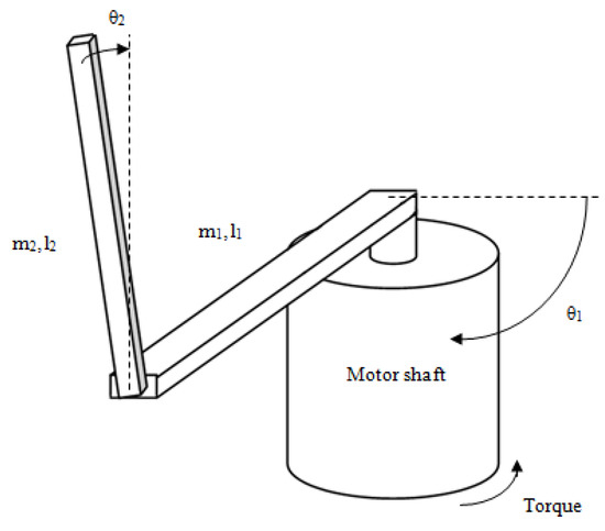
Figure 6. Rotary inverted pendulum.

Table 9. List of parameters of rotary inverted pendulum.

Name	Description	Value
$m_1$	Mass of arm	0.056 kg
$l_1$	Length of arm	0.16 m
$c_1$	Distance to arm center of mass	0.08 m
$J_1$	Inertia of arm	0.00215058 kg·m${}^2$
$m_2$	Mass of pendulum	0.022 kg
$l_2$	Length of pendulum	0.16 m
$c_2$	Distance to pendulum center of mass	0.08 m
$J_2$	Inertia of pendulum	0.00018773 kg·m${}^2$
$R_m$	Armature resistance	2.5604 $\mathsf{\Omega }$
$K_b$	Back-emf constant	0.01826 V·s/rad
$K_t$	Torque constant	0.01826 N·m/A
${\theta }_1$	Angular displacement of arm	-
${\theta }_1^{\prime }$	Angular velocity of arm	-
${\theta }_2$	Angular displacement of pendulum	-
${\theta }_2^{\prime }$	Angular velocity of pendulum	-
$\tau$	Applied torque	-

As long as the goal of the control was to set the pendulum to the upright position and the arm to the predefined zero position, the fitness calculation was based on the total difference between the desired and actual positions of the pendulum and the arm, as well as their angular velocity. So, the fitness was defined as follows:

$$f_i=\frac{1}{\pi }\sum _{j=0}^{\frac{T_{max}}{h}}|x{1}_j|+\frac{1}{\pi }\sum _{j=0}^{\frac{T_{max}}{h}}|x{2}_j|+\frac{1}{2}\sum _{j=0}^{\frac{T_{max}}{h}}|x{3}_j|+\frac{1}{20}\sum _{j=0}^{\frac{T_{max}}{h}}|x{4}_j|$$

(6)

Each state variable in fitness calculation was weighted by its range. The controller design consisted of four separate steps, where the goal of the first step was to stabilize the pendulum in an upright position, the second was to stabilize and bring an arm to the desired position, and the third and fourth were to repeat the same with swing-up sequence. The parameters of the starting points for the control are presented in Table 10.

Table 10. Starting positions for fitness evaluation.

Starting Position	x1	x2	x3	x4
1	0	−0.1	0	0
2	3	−0.1	0	0
3	0	1.41	0	0
4	3	1.41	0	0

The learning process was divided into four parts, the maximum number of generations was set to 2500, the population size was set to 100 individuals. To test the efficiency of the approach there were 10 independent runs of the algorithm performed. For every run, at each generation, the best individual was used to build the graphs of control.

First, the sensitivity analysis was performed for different values of mean, used in normal distribution for F sampling. The comparison results are shown in Table 11. The Mann–Whitney statistical tests were performed with the same parameters as for classification problems.

Table 11. $\mathit{NEAT}$ vs. ${\mathit{NEAT}}_{\mathit{DBM}}$ performance for RIP problem

Performance Value	NEAT	${\mathit{NEAT}}_{\mathit{DBM}0.1}$	${\mathit{NEAT}}_{\mathit{DBM}0.3}$	${\mathit{NEAT}}_{\mathit{DBM}0.5}$	${\mathit{NEAT}}_{\mathit{DBM}0.7}$	${\mathit{NEAT}}_{\mathit{DBM}0.9}$
Mean	416.68	422.35	383.37	372.25	408.57	454.24
Median	459.96	397.20	424.15	398.76	416.74	458.92
Std	104.60	54.98	106.66	122.46	61.34	30.69
Min	186.87	361.63	132.62	65.67	288.62	403.04
M-W test	-	0, Z = 0.45	0, Z = 1.36	0, Z = 1.06	0, Z = 1.36	0, Z = −0.15

According to the sensitivity analysis in Table the best results on average were achieved with the mean value in F sampling equal to 0.5, and the median value is the second smallest here. In this case, the best solution with the fitness of 65.67 was found, while the best solution of the original NEAT has a fitness equal to 186.87.

Figure 7 and Figure 8 show the best-obtained controller behavior by neuroevolution with difference-based mutation and the architecture of the trained net while, and Figure 9 and Figure 10 show the same without difference-based mutation.

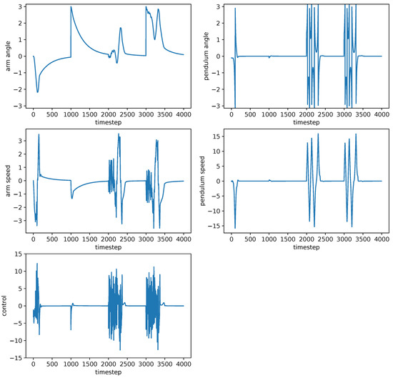
Figure 7. Pendulum dynamics with controller designed by neuroevolution without DBM.

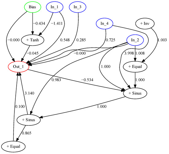
Figure 8. Best controller designed by neuroevolution without DBM.

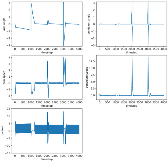
Figure 9. Pendulum dynamics with controller designed by neuroevolution with DBM.

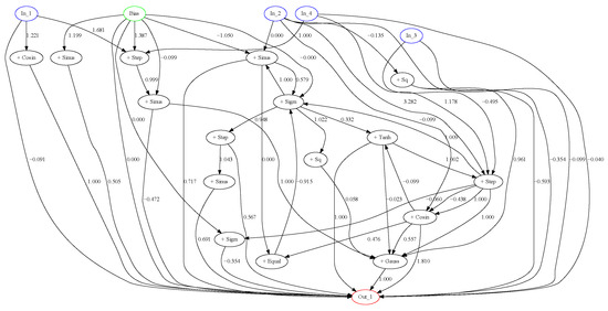
Figure 10. Best controller designed by neuroevolution with DBM.

Figure 7 shows that the controller designed without DBM was able to stabilize the pendulum itself in all four scenarios, however, it was not able to set the arm in the desired zero position or at least minimize its speed. However, the controller designed with DBM (Figure 8) was able to stabilize both the arm and the pendulum, although a small shift of the arm could be observed.

The architecture of the network, shown in Figure 10, contains a lot of connections and is relatively complex, compared to the architecture of the network, designed without distance-based mutation. This indicates that NEAT with DBM is capable of searching for optimal parameters more efficiently, and thus can build larger structures and tune them.

4. Conclusions

This study presented a new mutation operator for the well-known neuroevolution algorithm. The proposed difference-based mutation uses the innovation numbers stored in every connection in the NEAT architecture to find the corresponding ones, and performs mutation similar to the one used in differential evolution. The experiments performed on classification problems with sensitivity analysis have shown that NEAT with DBM shows superior performance compared to the original NEAT algorithm in several cases, and the results show that the best choice for the mean value for scaling factor sampling is 0.5. Moreover, the efficiency of NEAT-DBM is comparable to other well-known classification methods, and in several cases is even better. Testing on the rotary inverted pendulum control problem has shown that the NEAT-DBM algorithm allows finding better solutions with the same computational resource, and in the cases considered in this study, it was able to generate an almost ideal control algorithm. Further directions of studies may include applying the proposed difference-based mutation to other NEAT implementations and problems, which could be solved by it, as well as the development of other search operators, such as difference-based crossover.

References

- Bengio, Y.; LeCun, Y.; Hinton, G. Deep Learning. Nature 2015, 521, 436–444. [Google Scholar]
- Hochreiter, S.; Schmidhuber, J. Long Short-Term Memory. Neural Comput. 1997, 9, 1735–1780. [Google Scholar] [CrossRef]
- Jaeger, H.; Haas, H. Harnessing Nonlinearity: Predicting Chaotic Systems and Saving Energy in Wireless Communication. Science 2015, 304, 78–80. [Google Scholar] [CrossRef] [PubMed]
- Chenxi, L.; Zoph, B.; Neumann, M.; Shlens, J.; Hua, W.; Li, L.-J.; Fei-Fei, L.; Yuille, A.; Huang, J.; Murphy, K. Progressive Neural Architecture Search. In Proceedings of the European Conference on Computer Vision (ECCV 2018), Munich, Germany, 8–14 September 2018; pp. 19–34. [Google Scholar]
- Real, E.; Moore, S.; Selle, A.; Saxena, S.; Suematsu, Y.L.; Tan, J.; Le, Q.V.; Kurakin, A. Large-scale evolution of image classifiers. In Proceedings of the ICML, Sydney, Australia, 6–11 August 2017. [Google Scholar]
- Miikkulainen, R.; Liang, J.Z.; Meyerson, E.; Rawal, A.; Fink, D.; Francon, O.; Raju, B.; Shahrzad, H.; Navruzyan, A.; Duffy, N.; et al. Evolving deep neural networks. Neural Evol. Comput. 2017, 293–312. [Google Scholar] [CrossRef]
- Xie, L.; Yuille, A.L. Genetic CNN. In Proceedings of the IEEE International Conference on Computer Vision, Venice, Italy, 22–29 October 2017; pp. 1388–1397. [Google Scholar]
- Angeline, P.J.; Saunders, G.M.; Pollack, J.B. An evolutionary algorithm that constructs recurrent neural networks. IEEE Trans. Neural Netw. 1993, 5, 54–65. [Google Scholar] [CrossRef] [PubMed]
- Stanley, K.O.; Miikkulainen, R. Evolving Neural Networks through Augmenting Topologies. Evol. Comput. 2002, 10, 99–127. [Google Scholar] [CrossRef] [PubMed]
- Stanovov, V.; Akhmedova, S.; Semenkin, E. Neuroevolution of augmented topologies with difference-based mutation. IOP Conf. Ser. Mater. Sci. Eng. 2021, 1047, 012075. [Google Scholar] [CrossRef]
- Braun, H.; Weisbrod, J. Evolving feedforward neural networks. In Proceedings of the ANNGA93, International Conference on Artificial Neural Networks and Genetic Algorithms, Innsbruck, Austria, 14–16 April 1993; pp. 25–32. [Google Scholar]
- Dasgupta, D.; McGregor, D. Designing application-specific neural networks using the structured genetic algorithm. In Proceedings of the International Conference on Combinations of Genetic Algorithms and Neural Networks, Baltimore, MD, USA, 6 June 1992; pp. 87–96. [Google Scholar]
- Yao, X.; Liu, Y. Towards designing artificial neural networks by evolution. Appl. Math. Comput. 1996, 91, 83–90. [Google Scholar] [CrossRef]
- Floreano, D.; Durr, P. Mattiussi C Neuroevolution: From Architectures to Learning. Evol. Intell. 2008, 1, 47–62. [Google Scholar]
- Rodrigues, N.M.; Silva, S.; Vanneschi, L. A Study of Fitness Landscapes for Neuroevolution. In Proceedings of the IEEE Congress on Evolutionary Computation (CEC), Glasgow, UK, 19–24 July 2020; pp. 1–8. [Google Scholar]
- Arza, E.; Ceberio, J.; Pérez, A.; Irurozki, E. An adaptive neuroevolution-based hyperheuristic. In Proceedings of the 2020 Genetic and Evolutionary Computation Conference Companion (GECCO ’20), Cancún, Mexico, 8–12 July 2020; pp. 111–112. [Google Scholar]
- Gonzalez, S.; Miikkulainen, R. Improved Training Speed, Accuracy, and Data Utilization Through Loss Function Optimization. In Proceedings of the IEEE Congress on Evolutionary Computation (CEC), Glasgow, UK, 19–24 July 2020; pp. 1–8. [Google Scholar]
- Gomez, F.; Schmidhuber, J.; Miikkulainen, R. Accelerated Neural Evolution Through Cooperatively Coevolved Synapses. J. Mach. Learn. Res. 2008, 9, 937–965. [Google Scholar]
- Yaman, A.; Mocanu, D.C.; Iacca, G.; Fletcher, G.; Pechenizkiy, M. Limited evaluation cooperative co-evolutionary differential evolution for large-scale neuroevolution. In Proceedings of the Genetic and Evolutionary Computation Conference, Kyoto, Japan, 15–19 July 2018; pp. 569–576. [Google Scholar]
- Lyu, Z.; ElSaid, A.; Karns, J.; Mkaouer, M.W.; Desell, T. An Experimental Study of Weight Initialization and Lamarckian Inheritance on Neuroevolution. In EvoApplications Lecture Notes in Computer Science; Springer: Berlin/Heidelberg, Germany, 2021; Volume 12694. [Google Scholar] [CrossRef]
- Deb, K.; Deb, D. Analysing mutation schemes for real-parameter genetic algorithms. Int. J. Artif. Intell. Soft Comput. 2014, 4, 1–28. [Google Scholar] [CrossRef]
- Kennedy, J.; Eberhart, R. Particle Swarm Optimization. In Proceedings of the IEEE International Conference on NEURAL Networks, Perth, WA, Australia, 27 November–1 December 1995; pp. 1941–1948. [Google Scholar]
- Storn, R.; Price, K. Differential evolution—a simple and efficient heuristic for global optimization over continuous spaces. J. Glob. Optim. 1997, 11, 341–359. [Google Scholar] [CrossRef]
- Yang, X.S.; Deb, S. Cuckoo Search via Levy flights. In Proceedings of the World Congress on Nature & Biologically Inspired Computing, Coimbatore, India, 9–11 December 2009; pp. 210–214. [Google Scholar]
- Alcalá-Fdez, J.; Sánchez, L.; Garcia, S.; del Jesus, M.J.; Ventura, S.; Garrell, J.M.; Otero, J.; Romero, C.; Bacardit, J.; Rivas, V.M.; et al. KEEL: A software tool to assess evolutionary algorithms for data mining problems. Soft Comput. 2009, 13, 307–318. [Google Scholar] [CrossRef]
- Heaton, J. Ian Goodfellow, Yoshua Bengio, and Aaron Courville, Deep learning. Genet. Program. Evolvable Mach. 2015, 19, 305–307. [Google Scholar] [CrossRef]
- Quinlan, J.R. Bagging, boosting, and C4.5. AAAI/IAAI 1996, 1, 725–730. [Google Scholar]
- Breiman, L. Random forests. Mach. Learn. 2001, 45, 5–32. [Google Scholar] [CrossRef]
- Stanovov, V.; Semenkin, E.; Semenkina, O. Self-configuring hybrid evolutionary algorithm for fuzzy classification with active learning. In Proceedings of the IEEE Congress on Evolutionary Computation, Sendai, Japan, 24–28 May 2015; pp. 1823–1830. [Google Scholar]
- Stanovov, V.; Semenkin, E.; Semenkina, O. Self-configuring hybrid evolutionary algorithm for fuzzy imbalanced classification with adaptive instance selection. J. Artif. Intell. Soft Comput. Res. 2016, 6, 173–188. [Google Scholar] [CrossRef]
- Chollet, F. The Keras Library. 2015. Available online: https://keras.io (accessed on 20 April 2021).
- Pedregosa, F.; Varoquaux, G.; Gramfort, A.; Michel, V.; Thirion, B.; Grisel, O.; Blondel, M.; Prettenhofer, P.; Weiss, R.; Dubourg, V.; et al. Scikit-learn: Machine Learning in Python. J. Mach. Learn. Res. 2011, 12, 2825–2830. [Google Scholar]
- Prasad, L.B.; Tyagi, B.; Gupta, H.O. Optimal Control of Nonlinear Inverted Pendulum System Using PID Controller and LQR: Performance Analysis Without and With Disturbance Input. Int. J. Autom. Comput. 2011, 11, 661–670. [Google Scholar] [CrossRef]
- Fairus, M.A.; Mohamed, Z.; Ahmad, M.N. Fuzzy modeling and control of rotary inverted pendulum system using LQR technique. IOP Conf. Ser. Mater. Sci. Eng. 2013, 53, 1–11. [Google Scholar]
Publisher’s Note: MDPI stays neutral with regard to jurisdictional claims in published maps and institutional affiliations. |
© 2021 by the authors. Licensee MDPI, Basel, Switzerland. This article is an open access article distributed under the terms and conditions of the Creative Commons Attribution (CC BY) license (https://creativecommons.org/licenses/by/4.0/).