Abstract
Compared with continuous elements, discontinuous elements advance in processing the discontinuity of physical variables at corner points and discretized models with complex boundaries. However, the computational accuracy of discontinuous elements is sensitive to the positions of element nodes. To reduce the side effect of the node position on the results, this paper proposes employing partially discontinuous elements to compute the time-domain boundary integral equation of 3D elastodynamics. Using the partially discontinuous element, the nodes located at the corner points will be shrunk into the element, whereas the nodes at the non-corner points remain unchanged. As such, a discrete model that is continuous on surfaces and discontinuous between adjacent surfaces can be generated. First, we present a numerical integration scheme of the partially discontinuous element. For the singular integral, an improved element subdivision method is proposed to reduce the side effect of the time step on the integral accuracy. Then, the effectiveness of the proposed method is verified by two numerical examples. Meanwhile, we study the influence of the positions of the nodes on the stability and accuracy of the computation results by cases. Finally, the recommended value range of the inward shrink ratio of the element nodes is provided.
1. Introduction
Due to the advantages of dimensionality reduction, semi-analysis, and being suitable for dealing with stress concentration and infinite domain problems, the boundary element method (BEM) [1] has been successfully adopted in different environments, such as fracture mechanics [2,3,4] and acoustics [5,6,7,8]. In contrast to the finite element method (FEM) [9,10], the BEM does not require the continuity of physical quantities between elements [11]. This point can be confirmed from the successful application of constant boundary elements. Therefore, the BEM is adopted to analyze the elastodynamic problem in this paper.
According to the positions of the nodes, the boundary elements are classified as continuous (conforming) or discontinuous (non-conforming) elements. Continuous elements share common nodes with their neighbors, whereas discontinuous elements do not [12]. As discontinuous boundary elements have an advantage in processing the geometric corner and boundary conditions, they are widely employed in the BEM [13,14,15]. Moreover, the discontinuous element has good adaptability to the boundary shape of the analysis domain so that it is easy to realize the mesh discretization of complex models. However, the positions of nodes in the discontinuous element significantly affect the computational accuracy. Xu and Brebbia [16] first discussed the problem through the computation of the two-dimensional elastostatic problem and made the conclusion that the optimal position of the element node is determined by the Gauss–Legendre integration point. The research of Parreira [17] and Marburg [18] reached similar conclusions to Xu and Brebbia [16]. Manolis and Banerjee [19] also discussed the node position problem. They claimed that the nodes should be distributed as uniformly as possible in the discontinuous element. A similar conclusion can be found in [15].
Although the discontinuous element advances in processing the discontinuity of physical variables at corner points, the completely discontinuous element will significantly increase the number of nodes in the computation model, which increases the computational cost. Additionally, the computational accuracy of the completely discontinuous element is sensitive to the positions of element nodes, making the numerical results unstable. A better way to deal with the corner problem is to use partially discontinuous elements [20], in which only the nodes at the corner points are moved into the element, and the nodes at the non-corner points remain unchanged. Therefore, a discrete model that is continuous on surfaces and discontinuous between adjacent surfaces can be generated. Subia and Ingber [21] studied the influence of the position of the element node in partially discontinuous elements on computational accuracy based on the Laplace equation. Their results demonstrated that the computational accuracy is insensitive to the position of the element node when the distance moved inward is equal to [0.05, 0.3] times the edge length of the element. A similar conclusion can be found in [22], that is, the computational accuracy of the partially discontinuous element is less sensitive to the position of the element node. Moreover, the partially discontinuous element will not add too many nodes to the computation model, and the computational cost is comparable to that of the continuous element. Therefore, partially discontinuous boundary elements are employed to compute the 3D transient elastodynamic problems in this paper.
The BEM for solving elastodynamic problems [23] mainly includes the time-domain BEM, the frequency-domain BEM, and the double reciprocity BEM. For transient problems, the time-domain BEM is the most natural, direct, and applicable method. However, compared with the other two methods, the numerical stability of the time-domain BEM is poor. The computation results are easily affected by discrete parameters such as the time step and the element size [24,25,26]. In this paper, the time-domain BEM with partially discontinuous elements is introduced to compute 3D elastodynamic problems. The numerical implementation and performance of the partially discontinuous elements are studied. The main contributions of this paper can be summarized as follows:
- (1)
- The numerical integral scheme of the partially discontinuous elements is studied, in which the calculation of a singular integral [27,28,29] is carefully examined. An improved singular element subdivision method is proposed to reduce the side effect of the time step on the integral accuracy.
- (2)
- The influence of the node position of the partially discontinuous elements on the computational accuracy and result stability is studied through two classical numerical examples. The recommended value range of the inward shift ratio of the element node is provided.
The remainder of the paper is organized as follows: We introduce the boundary integral equation of 3D elastodynamics and its numerical implementation in Section 2. The numerical integral scheme of partially discontinuous elements together with the processing of the singular integral is described in Section 3. The experiments and analysis are shown in Section 4. Finally, we summarize the paper in the last section.
2. Time-Domain Boundary Integral Equation of Elastodynamics and Its Numerical Implementation
In this section, the time-domain boundary integral equation of elastodynamics and its numerical implementation are presented. As the basis of the research in this paper, the formulas shown in this section are well known and refer to the classic literature [23] in this field.
2.1. Time-Domain Boundary Integral Equation
The governing equation of the elastodynamic problem for homogeneous, isotropic, linear elastic materials [23] is
with boundary conditions
and initial conditions
in which the symbols used are as follows:
- i and j represent the three directions of the 3D space;
- ui represents the displacement component;
- pi represents the traction component in the i direction;
- bi represents the body force per mass;
- is the first-order derivative of displacement ui versus time t;
- is the second-order derivative of displacement ui versus time t;
- and represent the boundary displacement on and the boundary traction on , respectively, where the whole boundary ;
- V represents the whole domain of the analysis object;
- ρ is the medium density;
- λ and G are the Lame constants given bywhere E and ν represent Young’s modulus and Poisson’s ratio, respectively.
The time-domain boundary integral equation (BIE) corresponding to the governing Equation (1) can be expressed as
in which the meanings of the symbols used are as follows:
- when the source point p is located on smooth surfaces, and when the source point p is located in the domain ( when , otherwise );
- and are the time-dependent displacement fundamental solution and the traction fundamental solution, respectively, whose expressions can be found in [23];
- represents the velocity fundamental solution, which is the first-order derivative of versus time.
Assuming that the body force and initial conditions are both zero, Equation (5) can be simplified to
2.2. Numerical Implementation of the BIE
Equation (6) can be solved numerically by using the time step method to deal with the time integral and the collocation point method to process the space integral. If we discretize the time interval [0, t] into M time steps of duration Δt, the discretized time nodal , where M = 1, 2, …, N. Lagrange interpolation is used to approximate the dynamic response at any time in the discrete time interval [tM−1, tM]. In this paper, both displacement and traction adopt linear interpolation in the time interval, that is, for a specific time step M, the time interpolation formulas of displacement and traction are as follows:
in which
with
Substituting Equation (7) into Equation (6), the BIE of the time-discrete format can be obtained as follows:
The time integral in Equation (10) can be calculated analytically. After time integration, the BIE without the time variable τ can be obtained, as shown below:
in which and represent the displacement and traction kernel functions after time integration, respectively, and and represent the displacement and traction at the initial moment, respectively. Under zero initial conditions, = = 0.
After discretizing the boundary S into L elements, we use the K-th Lagrange interpolation function to formulate the BIE of the spatial discretization:
in which and , respectively, represent the displacement and traction at the k-th node in the l-th element at t = mΔt, and represents the shape function at the integration point q. Equation (12) can use the Gauss–Legendre quadrature method to perform numerical integration on each element. Then, the physical variables at all element nodes can be obtained by solving the linear equations derived from Equation (12).
In this paper, the spatial discretization of Equation (12) adopts partially discontinuous elements. As shown in Figure 1, the blue lines represent the boundary of the surface, the black lines represent the edges of the mesh elements, the hollow dots represent the original element nodes, and the red solid dots represent the element collocation points which are moved inward. The nodes located on the surface but not on the edges (such as black solid dots in Figure 1) remain unchanged. It can be seen that in the partially discontinuous element, only the nodes located at the corner points are shrunk to the surface, and other nodes remain unchanged. Therefore, the partially discontinuous element can avoid the discontinuity problem of physical variables at the corner points without adding too many nodes. It is a compromise between the continuous element and the completely discontinuous element.
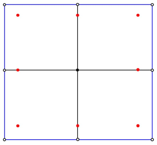
Figure 1.
Sketch map of the partially discontinuous element.
3. Numerical Integration Scheme of the Partially Discontinuous Element and the Treatment of the Singular Integral
In this section, the numerical integration scheme of the partially discontinuous element is presented according to [20,21,22]. To reduce the side effect of the time step on the singular integral accuracy, an improved singular element subdivision method is proposed in this section.
3.1. Numerical Integration Scheme
For convenience, we take the numerical integration of an element in Equation (12) as an example. The integral of the l-th element for the source point p is as follows:
in which or , represents the shape function of the partially discontinuous element. Equation (13) is usually numerically calculated by the Gauss–Legendre quadrature method. Before applying the Gauss–Legendre quadrature method to Equation (13), the coordinate system should be transformed from the real 3D space xyz to the regular space ξηw, as shown in Figure 2.
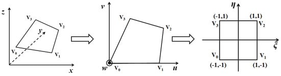
Figure 2.
Transformation of the coordinate system.
The transformation formula is formulated as follows:
where is the determinant of the Jacobian matrix of the transformation from the xyz space to the uvw space, and is the determinant of the Jacobian matrix of the transformation from the uvw space to the ξηw space. The calculation method of and in the partially discontinuous element is the same as that in the continuous element [1].
Since the interpolation points in partially discontinuous elements are the element nodes after inward shifting, the shape function is different from the standard shape function . As shown in Figure 3, dk is the position of node k after moving inside the element.
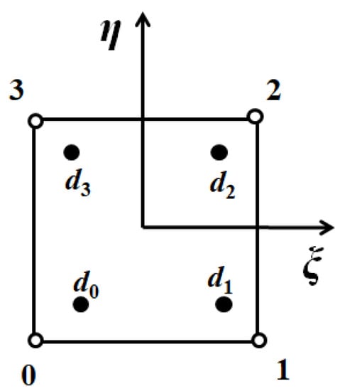
Figure 3.
Sketch map of interpolation points.
The physical variable at any point in the element can be calculated by the standard shape function as
The u at the interpolation point dk can be calculated by
which can be rewritten in a matrix form as follows:
We can reverse Equation (17) to obtain
Let
and substituting Equation (18) into Equation (15), we can obtain
where
The calculation formula of the new shape function can be obtained as shown in Equation (21). For the interpolation point dk that does not move inward, just take as the original node coordinates.
3.2. Singular Integral
In this paper, the coordinate transformation method combined [29] with an improved element subdivision method is adopted to deal with weakly singular integrals (f(1/r)), while the rigid body displacement method [23] is used to compute strongly singular integrals (f(1/r2)) indirectly. In the traditional element subdivision method, the integral element is divided into several triangular patches according to the position of the source point p, as shown in Figure 4. Then, the α–β transformation method [29] is used to eliminate the weak singularity in each patch.
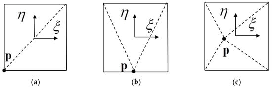
Figure 4.
The traditional element subdivision method: (a) p is located at the corner; (b) p is located on the edge; (c) p is located in the element.
However, the value of the fundamental solutions of elastodynamics is related to the time step. As shown in Figure 5, the curves of the displacement kernel function are different under different time steps. In Figure 5, r represents the distance between the source point p and the field point q. It can be seen that the function value changes rapidly when r < c2Δt, in which c2 represents the shear wave velocity and Δt represents the time step. The smaller the time step Δt, the more drastically the function value changes.
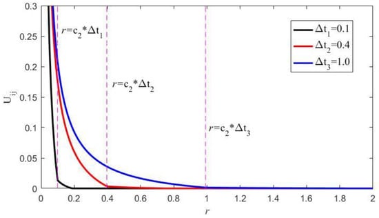
Figure 5.
The curve graph of the displacement kernel function under different time steps.
Therefore, this paper proposes an improved element subdivision scheme related to the time step as follows:
- (1)
- Create a square with the source point p as the center and 2 c2Δt as the side length. If the square exceeds the boundary of the element (as shown by the red dashed lines in Figure 6), the boundary of the element is taken as the boundary of the square;
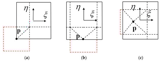 Figure 6. The improved element subdivision method: (a) p is located at the corner; (b) p is located on the edge; (c) p is located in the element.
 - (2)
- According to the position of the source point p and the square area established, the element is subdivided into several triangular patches containing p and quadrilateral patches without p, as shown by the black dashed lines in Figure 6;
- (3)
- The α–β transformation method is used for integrals on the triangular patches, and the standard Gauss–Legendre quadrature method is used on the quadrilateral patches.
Compared with the traditional element subdivision method, the improved element subdivision method related to the time step proposed in this paper can cause the Gauss points to be mainly distributed in the region of r < c2Δt (the region where the kernel function value changes drastically). Therefore, in the case of the same number of Gauss points, the improved subdivision method can significantly improve the accuracy of the singular integral. To verify the computational accuracy of the improved element subdivision method, a numerical example is given next to compare the computational accuracy before and after the improvement.
As shown in Figure 7, the coordinate of the source point p is (0, 0), and the coordinates of the quadrilateral element are shown in the figure. The dotted circles represent the boundaries of the wavefronts. The radius of the oscillation area changes with the time step Δt. Consider the following integral function:
where is the displacement kernel function after time integration. The material parameters in the function are defined as follows: Young’s modulus , density , and Poisson’s ratio . The average relative error of the integration result is defined as follows:
in which represents the reference result. In this example, the integration results of 50 * 50 Gauss points for each triangle patch and 25 * 25 Gauss points for each quadrilateral patch are used as reference results.
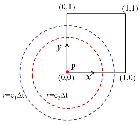
Figure 7.
Coordinates of the integration element and the source point.
With different time steps and different numbers of Gauss points, the errors of the integral results before and after the improvement are shown in Table 1. It can be seen that when the number of Gauss points used is the same, the computation error of the traditional element subdivision method becomes larger and larger as the time step Δt decreases. However, the computation error of the improved method can be kept at the same order of magnitude. In the case of the same time step, whether it is improved or not, the computation error will decrease as the number of Gauss points increases. In general, the computation error of the improved method is an order of magnitude less than that of the traditional method. Therefore, in the following computation examples of elastodynamic problems, we will use the improved element subdivision method to deal with singular integrals.

Table 1.
Computation errors of the element singular integral results.
4. Numerical Examples
In this section, two classical elastodynamic problems will be examined to verify the effectiveness of the proposed method. For the first example, the dynamic response of a cantilever beam under a longitudinal load is computed. The influence of the positions of element nodes on the computational stability and accuracy of the result is studied by cases. For the second example, the response of the plate with a square hole under a dynamic load is computed. The results under different inward shrink ratios are compared. According to the results of the two examples, the recommended value range of the inward shrink ratios of element nodes when using partially discontinuous elements is given.
4.1. Longitudinal Forced Vibration of a Cantilevered Beam
The geometric model used in this example is shown in Figure 8. The left end of the beam is fixed, and the right end is subjected to a Heaviside-type load p(t) = 1000 H(t) Pa. The material parameters of the beam are Young’s modulus , density , and Poisson’s ratio .
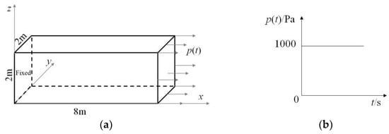
Figure 8.
The geometric model and the boundary conditions of the beam: (a) geometric model; (b) load curve.
By setting , the problem in this example can be regarded as the longitudinal forced vibration of a one-dimensional rod. The analytical solutions to the problem are available. The displacement solution and the internal force solution can be calculated by the formulas
and
respectively, where is the wave speed.
The discretized mesh model is shown in Figure 9a, which includes 72 linear quadrilateral elements and 126 nodes. In this model, the nodes located at the corner points are shrunk to the surfaces in proportion (as shown in Figure 9b), where a represents the moving distance of the node and b represents the edge length of the element.
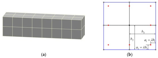
Figure 9.
The mesh model of the beam: (a) mesh model; (b) inward shrink ratio λ.
The computation results of the time-domain BEM are sensitive to the time step. An improper time step length will cause the results to diverge, which is unstable. Therefore, in many papers [24,25,26], the time step is selected according to the dimensionless parameters , where is the pressure wave velocity, is the time step, and d is the element edge length. The smaller the value of β is, the more unstable the result will be. The larger the value of β is, the lower the computational accuracy. In general, acceptable results can be obtained when . In this experiment, we choose the time step that can obtain stable results for computation. On this basis, the influence of the inward shrink ratio of the element node on the computation result is investigated.
When , the displacement response at the free end and the traction response at the fixed end under different λ values are shown in Figure 10 and Figure 11, respectively. In these two figures, the left picture and the right picture show unstable results and stable results, respectively. It can be seen that the results are unstable when and . The results are stable when , and the result curves overlap each other in these cases. Therefore, the value of should avoid being too large or too small, and the computational accuracy is insensitive to the value of λ if the results converge.
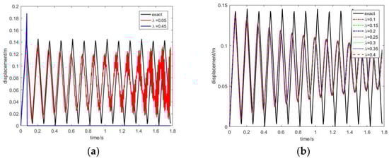
Figure 10.
Displacement response at the free end computed by using partially discontinuous elements in terms of (a) the cases of unstable results and (b) the cases of stable results.
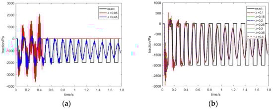
Figure 11.
Traction response at the fixed end computed by using partially discontinuous elements in terms of (a) the cases of unstable results and (b) the cases of stable results.
Under the same conditions, if completely discontinuous elements are used for discretization, the mesh model contains 72 linear quadrilateral elements and 288 nodes, which are greater values than those using partially discontinuous elements. The displacement response at the free end and the traction response at the fixed end under different λ values are shown in Figure 12 and Figure 13, respectively. It can be seen that the results tend to be stable only when , and the results are unstable in other cases. This demonstrates that the performance of the completely discontinuous element is very sensitive to the position of the element node. An inappropriate node inward shrink ratio can easily cause unstable results, so it is not suitable for the time-domain BEM.
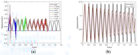
Figure 12.
Displacement response at the free end computed by using completely discontinuous elements in terms of (a) the cases of unstable results and (b) the cases of stable results.
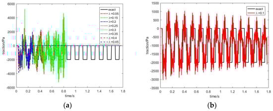
Figure 13.
Traction response at the fixed end computed by using completely discontinuous elements in terms of (a) the cases of unstable results and (b) the cases of stable results.
In order to verify the effectiveness of the improved singular element subdivision method proposed in Section 3.2, we compared the accuracy of the results before and after the improvement. It should be mentioned that the partially discontinuous element is adopted in the following study. Since the singular integral only appears in the first analysis step, we select the results of the first ten analysis steps to clearly observe the difference between the results before and after the improvement. The comparison results under the time steps , , and are shown in Figure 14a–c, respectively. In the figures, the “Exact” curve represents the exact solution, the “Traditional” curve represents the results before the improvement, and the “Improved” curve represents the results after the improvement. It can be seen that the improved results are in better agreement with the exact solutions. The results before the improvement become unstable as the time step decreases. This demonstrates that the improved singular element subdivision method can reduce the side effect of the time step on the stability of the result and effectively improve the accuracy of the singular integration. However, it should be noted that although the proposed subdivision method has improved the result accuracy in the first ten steps, the computational error becomes larger and larger with the accumulation of time steps, and instability results may still appear. The subdivision method proposed in this paper cannot completely solve the stability problem of the time-domain BEM but can improve the stability of the result.
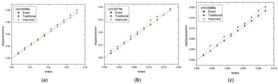
Figure 14.
The comparison results before and after the improvement of the singular element subdivision method under the time steps of (a) , (b) , and (c) .
Finally, the condition number of matrix A in Equation (21) with a different inward shrink ratio λ is studied. The condition number of matrix A is computed by
in which represents the two-norm of matrix A.
Three common types of discontinuous element are considered, as shown in Figure 15. In the figure, case 1 shows that four nodes are shrunk into the element, case 2 shows that three nodes are shrunk into the element, and case 3 shows that two nodes are shrunk into the element. Case 1 corresponds to the completely discontinuous element, and cases 2 and 3 correspond to the partially discontinuous element. Through computing the condition number of matrix A in Equation (21) with a different inward shrink ratio λ, Figure 16 is plotted for a results comparison. From Figure 16, the following can be seen:
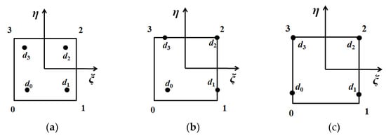
Figure 15.
Three types of discontinuous element: (a) case 1; (b) case 2; (c) case 3.
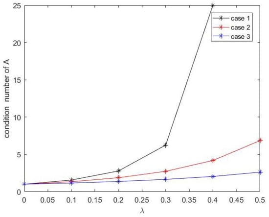
Figure 16.
The condition numbers of matrix A under a different inward shrink ratio λ.
(1) When the λ = 0, the condition number is equal to 1. The condition number of A becomes larger as the value of λ increases. In case 1, the matrix A becomes singular when λ = 0.5. The result verifies the conclusion that the value of λ should not be too large.
(2) The condition numbers of A in case 1 are larger than those in the other two cases. This verifies the conclusion that the result stability of the completely discontinuous element (corresponding to case 1) is poorer than that of the partially discontinuous element (corresponding to case 2 and case 3).
Figure 10 and Figure 11 show that when the value of λ is too small, the result will also be unstable. However, from the point of view of the condition number of A, the smaller the value of λ, the smaller the condition number, which is inconsistent with the experimental results. The reason may be that a too small value of λ will reduce the accuracy of the nearly singular integration. In fact, many discrete parameters other than the value of λ, such as the element size, interpolation type, and time step, will affect the stability of the result. Further in-depth research is needed to solve the instability problem of the time-domain BEM.
4.2. Response of a Plate with a Square Hole under Dynamic Load
In this example, a more realistic problem, which is the dynamic response of a plate with a square hole under an impact load, is computed. The geometric model used in this example is shown in Figure 17. The bottom of the plate is fixed, and the top is subjected to an impact loading Pa. The material parameters of the plate are Young’s modulus , density , and Poisson’s ratio . The dynamic responses at points S1 and S2 in Figure 17a are computed in this example.
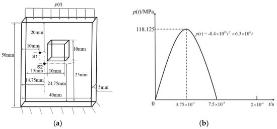
Figure 17.
The geometric model and the boundary conditions of the plate: (a) geometric model; (b) load curve.
The discretized mesh model with an element size of 5 mm is shown in Figure 18a. The exact solution of this example cannot be derived, so we adopt the results computed by FEM software to be the reference solution. The FEM mesh model is shown in Figure 18b, which uses a finer mesh model to ensure the reliability of the results.
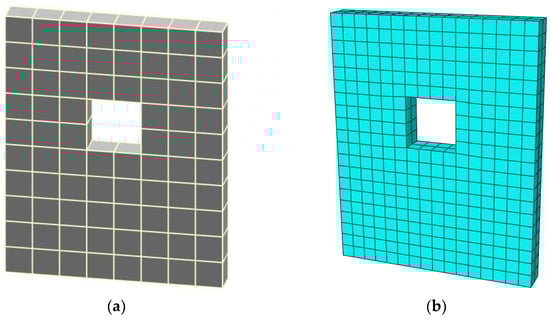
Figure 18.
The mesh model of the plate: (a) BEM mesh model; (b) FEM mesh model.
When , the displacement response and the traction response at point S1, which is next to the hole and denoted in Figure 17a, under different λ values are shown in Figure 19 and Figure 20, respectively. It can be seen from these figures that the results are stable when , and the result curves overlap each other in these cases. In other cases, the results are unstable. Therefore, a conclusion similar to the previous example can be obtained: the value of λ should avoid being too large or too small, and the computational accuracy is insensitive to the value of λ if the results converge. In this example, the value range of λ for stable results is smaller than that in the previous example. The reason is that the boundary of the geometric model in this example is more complicated than that in the previous example. Therefore, instability is more likely to occur in this example, and it is more stringent for the selection of the value of λ.
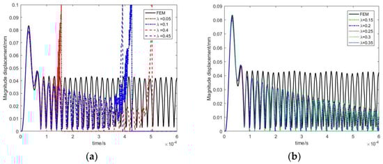
Figure 19.
Displacement response at point S1 computed by using partially discontinuous elements in terms of (a) the cases of unstable results and (b) the cases of stable results.
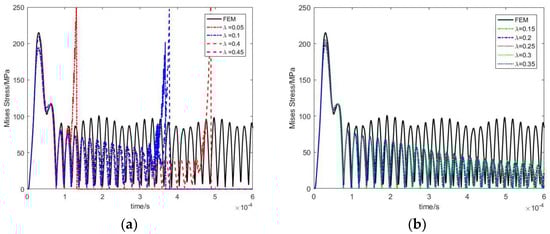
Figure 20.
Traction response at point S1 computed by using partially discontinuous elements in terms of (a) the cases of unstable results and (b) the cases of stable results.
Similarly, the displacement and traction responses at point S2, which is next to the corner of the square hole, are shown in Figure 21 and Figure 22, respectively. It can be seen that the results are stable when , and the result curves overlap each other in these cases. In other cases, the results are unstable. The results of point S2 are similar to the results of point S1.
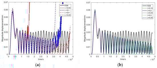
Figure 21.
Displacement response at point S2 computed by using partially discontinuous elements in terms of (a) the cases of unstable results and (b) the cases of stable results.
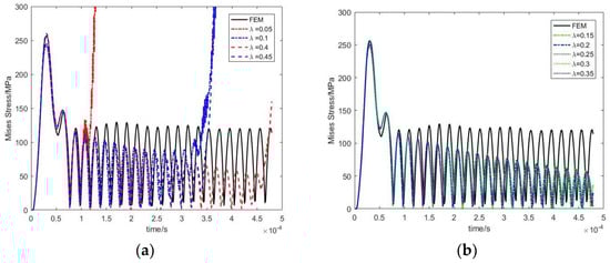
Figure 22.
Traction response at point S2 computed by using partially discontinuous elements in terms of (a) the cases of unstable results and (b) the cases of stable results.
From the figures of the results comparison in this section, it can be seen that the time-domain BEM can achieve high computational accuracy in the initial stage of computation. However, the numerical damping becomes larger and larger as the number of analysis steps increases, that is, the computational accuracy becomes lower and lower. There are two main reasons for this phenomenon: one is that the large time step adopted in the time-domain BEM computation leads to a lower accuracy of the result, while the result may not converge when the time step is small; the other is that the fundamental solutions of the time-domain BEM for elastodynamic problems are discontinuous piecewise functions, which leads to the element integral accuracy being low. The result error accumulates continuously as the number of analysis steps increases, resulting in lower and lower computational accuracy. The above two points are the difficulties to be overcome when using the time-domain BEM. They are also the reasons why the time-domain BEM is more suitable for calculating short-term dynamic responses such as explosions and shocks rather than long-term dynamic responses. The algorithm proposed in this paper can improve the computational stability and accuracy of the time-domain BEM to a certain extent. However, further research is needed to thoroughly solve the above two problems.
5. Conclusions
To treat the corners of body surfaces in a simple manner while restricting the number of nodes, we adopted partially discontinuous elements, which are continuous on surfaces and discontinuous between adjacent surfaces, to discretize the boundary of the model for solving the elastodynamic problems. The effects of the numerical integration scheme of the partially discontinuous element and the positions of collocation points on the stability and accuracy of the computational results were studied. We found the following:
(1) The computational accuracy of the singular integral is sensitive to the time step. For instance, the traditional singular integration scheme cannot obtain reliable results in the case where the value of the time step adopted is small. The proposed improved singular element subdivision method takes the time step into consideration, which significantly reduces the side effect of the time step on the accuracy of the singular integral. Meanwhile, it will not introduce too many Gauss points’ numbers. The proposed singular element subdivision method can improve the stability and accuracy of the dynamic response results in a short time. However, the accumulated error becomes larger and larger as the number of analysis steps increases, which leads to the rapid damping of the amplitude of the result.
(2) The effects of the node position in the completely discontinuous element and the partially discontinuous element on the results were compared. In terms of the stability of the computation results, the partially discontinuous element has obvious advantages over the completely discontinuous element. In terms of computational accuracy, the accuracy of the results of the partially discontinuous elements is more stable than that of the completely discontinuous elements and insensitive to the node position.
(3) When using the discontinuous element, the inward shrink ratio of the element node should be carefully determined. Otherwise, it may cause unstable results. For partially discontinuous elements, the recommended value range of the inward shrink ratio is [0.15, 0.3] in the case of adopting linear quadrilateral elements. It should be noted that the more complex the model boundary, the smaller the available range of the inward shrink ratio.
Author Contributions
Conceptualization, Y.L., W.M.; methodology, Y.L.; software, Y.L.; validation, Y.L., N.Z., Y.G.; formal analysis, Y.L.; data curation, N.Z., S.Z.; writing—original draft preparation, Y.L.; writing—review and editing, Y.G., W.M.; visualization, N.Z., S.Z.; project administration, Y.L.; funding acquisition, Y.L., W.M., S.Z. All authors have read and agreed to the published version of the manuscript.
Funding
This research was funded by the National Natural Science Foundation of China (Nos. 11702087, U1704158), and the Key Research Project of Higher School of Henan Province (No. 21A520020).
Data Availability Statement
Not Applicable, the study does not report any data.
Conflicts of Interest
The authors declare no conflict of interest.
References
- Brebbia, C.A. The Boundary Element Method for Engineers; Pentech Press: London, UK, 1978. [Google Scholar]
- Giannella, V. Stochastic approach to fatigue crack-growth simulation for a railway axle under input data variability. Int. J. Fatigue 2021, 144, 106044. [Google Scholar] [CrossRef]
- Citarella, R.; Buchholz, F.-G. Comparison of crack growth simulation by DBEM and FEM for SEN-specimens undergoing torsion or bending loading. Eng. Fract. Mech. 2008, 75, 489–509. [Google Scholar] [CrossRef]
- Citarella, R.; Cricrì, G. Comparison of DBEM and FEM Crack Path Predictions in a notched Shaft under Torsion. Eng. Fract. Mech. 2010, 77, 1730–1749. [Google Scholar] [CrossRef]
- Citarella, R.; Federico, L. Advances in Vibroacoustics and Aeroacustics of Aerospace and Automotive Systems. Appl. Sci. 2018, 8, 366. [Google Scholar] [CrossRef]
- Citarella, R.; Federico, L.; Barbarino, M. Aeroacustic and Vibroacoustic Advancement in Aerospace and Automotive Systems. Appl. Sci. 2020, 10, 3853. [Google Scholar] [CrossRef]
- Chen, L.L.; Lian, H.; Liu, Z.; Chen, H.B.; Atroshchenko, E.; Bordas, S. Structural shape optimization of three dimensional acoustic problems with isogeometric boundary element methods. Comput. Methods Appl. Mech. Eng. 2019, 355, 926–951. [Google Scholar] [CrossRef]
- Chen, L.; Lu, C.; Lian, H.; Liu, Z.; Bordas, S. Acoustic topology optimization of sound absorbing materials directly from subdivision surfaces with isogeometric boundary element methods. Comput. Methods Appl. Mech. Eng. 2020, 362, 112806. [Google Scholar] [CrossRef]
- Hughes, T.J.R. The Finite Element Method: Linear Static and Dynamic Finite Element Analysis; Prentice Hall: Upper Saddle River, NJ, USA, 2000. [Google Scholar]
- Armentani, E.; Giannella, V.; Citarella, R.; Parente, A.; Pirelli, M. Substructuring of a Petrol Engine: Dynamic Characterization and Experimental Validation. Appl. Sci. 2019, 9, 4969. [Google Scholar] [CrossRef]
- Perrella, M.; Gerbino, S.; Citarella, R. BEM in Biomechanics: Modelling Advances and Limitations, Book Chapter in Numerical Methods and Advanced Simulation in Biomechanics and Biological Processes; Academic Press: New York, NY, USA, 2017. [Google Scholar]
- Karur, S.; Ramachandran, P. Orthogonal collocation in the nonconforming boundary element method. J. Comput. Phys. 1995, 121, 373–382. [Google Scholar] [CrossRef]
- Trevelyan, J. Use of discontinuous boundary elements for fracture mechanics analysis. Eng. Anal. Bound. Elem. 1992, 10, 353–358. [Google Scholar] [CrossRef]
- Yerli, H.R.; Deneme, I.O. Elastodynamic boundary element formulation employing discontinuous curved elements. Soil Dyn. Earthq. Eng. 2008, 28, 480–491. [Google Scholar] [CrossRef]
- Sun, Y.; Trevelyan, J.; Hattori, G.; Lu, C. Discontinuous isogeometric boundary element (IGABEM) formulations in 3D automotive acoustics. Eng. Anal. Bound. Elem. 2019, 105, 303–311. [Google Scholar] [CrossRef]
- Xu, J.M.; Brebbia, C.A. Optimum positions for the nodes in discontinuous boundary elements. In Proceeding of the 8th Conference on Boundary Elements, Tokyo, Japan, 8 September 1986; pp. 751–767. [Google Scholar]
- Parreira, P. On the accuracy of continuous and discontinuous boundary elements. Eng. Anal. 1988, 5, 205–211. [Google Scholar] [CrossRef]
- Marburg, S.; Schneider, S. Influence of Element Types on Numeric Error for Acoustic Boundary Elements. J. Comput. Acoust 2008, 11, 363–386. [Google Scholar] [CrossRef]
- Manolis, G.D.; Banerjee, P.K. Conforming versus non-conforming boundary elements in three-dimensional elastostatics. Int. J. Numer. Meth. Eng. 1986, 23, 1885–1904. [Google Scholar] [CrossRef]
- Patterson, C.; Elsebai, N.A.S. A family of partially discontinuous boundary element for three-dimensional analysis. In Proceeding of the 5th Conference on Boundary Elements, Hiroshima, Japan, 8–11 November 1983; pp. 193–206. [Google Scholar]
- Subia, S.R.; Ingber, M.S.; Mitra, A.K. A comparison of the semidiscontinuous element and multiple node with auxiliary boundary collocation approaches for the boundary element method. Eng. Anal. Bound. Elem. 1995, 15, 19–27. [Google Scholar] [CrossRef]
- Sun, L.; Teng, B.; Liu, C.F. Removing irregular frequencies by a partial discontinuous higher order boundary element method. Ocean Eng. 2008, 35, 920–930. [Google Scholar] [CrossRef]
- Manolis, G.D.; Beskos, D.E. Boundary Element Method in Elastodynamics; Spon Press: London, UK, 1988. [Google Scholar]
- Frangi, A.; Novati, G. On the numerical stability of time-domain elastodynamic analyses by BEM. Comput. Methods Appl. Mech. Eng. 1999, 173, 403–417. [Google Scholar] [CrossRef]
- Marrero, M.; Dominguez, J. Numerical behavior of time domain BEM for three-dimensional transient elastodynamic problem. Eng. Anal. Bound. Elem. 2003, 27, 39–48. [Google Scholar] [CrossRef]
- Bai, X.; Pak, R.Y.S. On the stability of direct time-domain boundary element methods for elastodynamics. Eng. Anal. Bound. Elem. 2018, 96, 138–149. [Google Scholar] [CrossRef]
- Gao, X.W.; Zhang, J.B.; Zheng, B.J.; Zhang, C. Element-subdivision method for evaluation of singular integrals over narrow strip boundary elements of super thin and slender structures. Eng. Anal. Bound. Elem. 2016, 66, 145–154. [Google Scholar] [CrossRef]
- Xie, G.; Zhong, Y.; Zhou, F.; Du, W.; Zhang, D. Singularity cancellation method for time-domain boundary element formulation of elastodynamics: A direct approach. Appl. Math. Model. 2020, 80, 647–667. [Google Scholar] [CrossRef]
- Qin, X.; Zhang, J.; Li, G.; Sheng, X.; Song, Q.; Mu, D. An element implementation of the boundary face method for 3D potential problems. Eng. Anal. Bound. Elem. 2010, 34, 934–943. [Google Scholar] [CrossRef]


Publisher’s Note: MDPI stays neutral with regard to jurisdictional claims in published maps and institutional affiliations. |
© 2021 by the authors. Licensee MDPI, Basel, Switzerland. This article is an open access article distributed under the terms and conditions of the Creative Commons Attribution (CC BY) license (https://creativecommons.org/licenses/by/4.0/).