Safe Approximation—An Efficient Solution for a Hard Routing Problem

Abstract

The Disjoint Connecting Paths problem and its capacitated generalization, called Unsplittable Flow problem, play an important role in practical applications such as communication network design and routing. These tasks are NP-hard in general, but various polynomial-time approximations are known. Nevertheless, the approximations tend to be either too loose (allowing large deviation from the optimum), or too complicated, often rendering them impractical in large, complex networks. Therefore, our goal is to present a solution that provides a relatively simple, efficient algorithm for the unsplittable flow problem in large directed graphs, where the task is NP-hard, and is known to remain NP-hard even to approximate up to a large factor. The efficiency of our algorithm is achieved by sacrificing a small part of the solution space. This also represents a novel paradigm for approximation. Rather than giving up the search for an exact solution, we restrict the solution space to a subset that is the most important for applications, and excludes only a small part that is marginal in some well-defined sense. Specifically, the sacrificed part only contains scenarios where some edges are very close to saturation. Since nearly saturated links are undesirable in practical applications, therefore, excluding near saturation is quite reasonable from the practical point of view. We refer the solutions that contain no nearly saturated edges as safe solutions, and call the approach safe approximation. We prove that this safe approximation can be carried out efficiently. That is, once we restrict ourselves to safe solutions, we can find the exact optimum by a randomized polynomial time algorithm.

1. Introduction

In communication network design and routing, one often looks for disjoint routes that connect various sources with associated terminals. This motivates the Disjoint Connecting Paths problem, which is the following decision task:

Input: a set of source-destination node pairs $(s_1,t_1),\dots ,(s_k,t_k)$ in a graph.

Task: Find edge disjoint paths $P_1,\dots ,P_k$, such that $P_i$ connects $s_i$ with $t_i$ for each i.

This is one of the classical NP-complete problems that appears already at the sources of NP-completess theory, among the original problems of Karp [1]. It remains NP-complete both for directed and undirected graphs, as well as for the edge disjoint and vertex disjoint paths version. The corresponding natural optimization problem, when we are looking for the maximum number of terminator pairs that can be connected by disjoint paths is NP-hard.

There is also a capacitated version of the Disjoint Connecting Paths problem, also known as the Unsplittable Flow problem. In this task a flow demand is given for each origin-destination pair $(s_i,t_i)$, as well as a capacity value is known for each edge. The requirement is to find a system of paths, connecting the respective source-destination pairs and carrying the respective flow demands, such that the capacity constraint of each edge is obeyed, that is, the sum of the flows of paths that traverse the edge cannot be more than the capacity of the edge. The name Unsplittable Flow expresses the requirement that between each source-destination pair the flow must follow a single route, it cannot split. Note that the disjointness of the paths themselves is not required a priori in the Unsplittable Flow, but can be enforced by the capacity constraints, if needed. The Unsplittable Flow problem is widely regarded as a fundamental task in communication network design and routing applications. Note that it directly subsumes the Disjoint Connecting Paths problem as a special case, which can be obtained by taking all capacities and flow demands equal to 1.

In this paper, after reviewing some existing results, we show that the Unsplittable Flow problem, which is known to be NP-hard (and its decision version is NP-complete), becomes efficiently solvable if we impose a mild and practically well justifiable restriction. Specifically, our key idea is that we “cut down” a small part of the solution space by slightly reducing the edge capacities. In other words, we exclude solutions that are close to saturating some edges, which would be practically undesirable, anyway. We call remaining solutions safe solutions: safe in the sense that no link is very close to saturation. Why is this slight capacity reduction useful? Its usefulness is based on the fact, which we constructively prove in the paper, that if we restrict ourselves to safe solutions only, then the hard algorithmic problem becomes solvable by a relatively simple randomized polynomial time algorithm. With very high probability the algorithm finds the exact optimum in polynomial time, whenever there exists a safe solution. We call this approach safe approximation.

2. Previous Results

Considerable work was done on the Disjoint Connecting Paths problem, since its first appearance as an NP-complete task in the classic paper of Karp [1] in 1972.

One direction of research deals with finding the “heart” of the difficulty—the simplest restricted cases that still remain NP-complete. (Or NP-hard if the optimization version is considered, where we look for the maximum number of connecting paths, allowing that possibly not all source-destination pairs will be connected). Kramer and van Leeuwen [2] proves, motivated by VLSI layout design, that the problem remains NP-complete even for graphs as regular as a two dimensional mesh. If we restrict ourselves to undirected planar graphs with each vertex having degree at most three, the problem also remains NP-complete, as proven by Middendorf and Pfeiffer [3]. The optimization version remains NP-hard for trees with parallel edges, although there the decision problem is already solvable in polynomial time [4].

The restriction that we only allow paths which connect each source node with a dedicated target is essential. If this is relaxed and we are satisfied with edge disjoint paths that connect each source $s_i$ with some of destinations $t_j$ but not necessarily with $t_i,$ then the problem becomes solvable with classical network flow techniques. Thus, the prescribed matching of sources and destinations causes a dramatic change in the problem complexity. Interestingly, it becomes already NP-complete if we require that just one of the sources is connected to a dedicated destination, the rest is relaxed as above (Faragó [5]).

Another group of results produces polynomial time algorithmic solutions for finding the paths, possibly using randomization, in special classes of graphs. For example, Middendorf and Pfeiffer [3] proves the following. Let us represent the terminator pairs by demand edges. These are additional edges that connect a source with its destination. If this extended graph is embeddable in the plane such that the demand edges lie in a bounded number of faces of the original graph, then the problem is solvable in polynomial time. (The faces are the planar regions bordered by the curves that represent the edges in the planar embedding, that is, in drawing the graph in the plane). Thus, this special case requires that, beyond the planarity of the extended graph, the terminators are concentrated in a constant number of regions (independent of the graph size), rather than spreading over the graph.

Broder, Frieze, Suen and Upfal [6] consider the case of random graphs and provide a randomized algorithm that, under some technical conditions, finds a solution with high probability in time O(nm${}^2$) for a random graph of n vertices and m edges.

A deep theoretical result, due to Robertson and Seymour [7], is that for general undirected graphs the problem can be solved in polynomial time if the number k of paths to be found is constant (i.e., cannot grow with the size of the graph). This is important from the theoretical point of view, but does not lead to a practical algorithm, as analyzed by Bienstock and Langston [8]. On the other hand, for directed graphs the problem becomes NP-complete already for the smallest nontrivial case of $k=2$, as proven by Even, Itai, and Shamir [9].

Another line of research aims at finding approximations to the optimization version. An algorithm is said to be an $f\left(n\right)$-approximation if it can connect a subset of the terminator pairs by disjoint paths such that this subset is at most $f\left(n\right)$ times smaller than the optimum in a graph of n vertices. For example, in this terminology a 2-approximation algorithm always reaches at least the half of the optimum, or an $O(logn)$-approximation reaches at least a $c/logn$ fraction of the optimum, for $n>n_0$ with some constants $c,n_0.$

Various approximations have been presented in the literature. For example, Garg, Vazirani and Yannakakis [4] provide a 2-approximation for trees with parallel edges. Aumann and Rabani [10] gives an $O(logn)$-approximation for the 2-dimensional mesh. Kleinberg and Tardos [11] present an $O(logn)$-approximation for a larger subclass of planar graphs, they call “nearly Eulerian, uniformly high-diameter planar graphs.”

On the other hand, finding a constant factor, or at least a logarithmic factor approximation for general directed graphs is hopeless—Guruswami, Khanna, Rajaraman, Shepherd, and Yannakakis [12] showed that on directed graphs it is NP-hard to obtain an $O\left(n^{1/2-ϵ}\right)$ approximation for n-vertex graphs for any $ϵ>0$.

For the general case the approximation factor of $min\{\sqrt{m},m/o pt\}=O\left(\sqrt{m}\right)$ is known to be achievable (Srinivasan [13]), where m is the number of edges and $opt$ is the optimum, that is, the maximum number of disjoint connecting paths between the source-destination pairs. Similar bounds apply for the Unsplittable Flow problem, as well. Bounds have been also found in terms of special (less trivial) graph parameters. For example, Kolman and Scheideler [14] proves that an efficient $O\left(F\right)$ approximation exists, where F is the so called flow number of the graph. Although the flow number can be computed in polynomial time [14], it is a rather indirect characterization of the graph. Numerous further related results are reviewed in the Handbook of Approximation Algorithms and Metaheuristics [15].

It is worth noting that in the capacitated version (Unsplittable Flow problem) the approximation does not mean approximating the total carried flow. It is meant with respect to the number of source-destination pairs connected, such that for each pair their entire demand is carried. For example, if there are 30 source-destination pairs, each with flow demand four units, then a 2-approximation means routing at least 15 of these flows, each path carrying four units of flow. In other words, not only the paths are unsplittable, but also the flow demands. That is, if we connect all 30 source-destination pairs, but each route can carry only two units of flow, it would not count as a 2-approximation.

In summary, the landscape of the Disjoint Connecting Path and the Unsplittable Flow problems can be characterized by the following facts:

• The decision problems are NP-complete for the general case.
• The approximation versions are NP-hard for the general case, even within a large approximation factor.
• Polynomial time solutions or better approximations exist only for special cases.
• Even in those cases when a polynomial time solution exists, it is either far from practical, or else it applies to a graph class that is too special to satisfy the demands of network design applications.

3. The Method of Safe Approximation

The various above referenced solutions tend to be rather complicated, which is certainly not helpful for real-life applications, in particular for large, complex networks. Our approach for providing a more practical solution to the unsplittable flow problem based on the following idea. We “cut down” a small part of the solution space by slightly reducing the edge capacities. In other words, we exclude solutions that are close to saturating some edges, as explained below.

Let $V_i$ be the given flow demand of the $i^{\mathrm{th}}$ connecting path. We normalize these demands such that $V_i\le 1$ for every i. Let $C_j$ be the capacity of edge $j.$ The graph is assumed directed and the edges are numbered from 1 through m. Recall that a feasible solution of the problem is a set of $s_i-t_i$ (directed) paths, one for each i, satisfying the edge capacity constraints. The latter means that on each edge j the sum of the $V_i$ values of those paths that traverse the edge does not exceed $C_j.$ As mentioned earlier, deciding whether a feasible solution exist at all is a hard (NP-complete) problem.

On the other hand, not all feasible solutions are equally good from a practical viewpoint. For example, if a route system in a network saturates or nearly saturates some links, then it is not preferable because it is close to being overloaded. For this reason, let us assign a parameter $0<{\rho }_j<1$ to each edge $j,$ such that ${\rho }_j$ will act as a safety margin for the edge. More precisely, let us call a feasible solution a safe solution with parameters ${\rho }_j,j=1,\dots ,m,$ where m is the number of edges, if it uses at most ${\tilde{C}}_j={\rho }_j{C}_j$ capacity on edge $j.$ The parameter ${\rho }_j$ will be close to 1 in the cases that are interesting to us.

Now, the appealing thing is that if we restrict ourselves to only those cases when a safe solution exists, then the hard algorithmic problem becomes solvable by a relatively simple randomized polynomial time algorithm. With very high probability, the algorithm finds the exact optimum in polynomial time, whenever there exists a safe solution. We call this approach safe approximation.

The price is that we exclude those cases when a feasible solution might still possibly exists, but there is no safe solution. This means, in these cases all feasible solutions are undesirable, because they all make some edges nearly saturated. In these marginal cases the algorithm may find no solution at all. Our approach constitutes a new avenue to approximation, in the sense that instead of giving up finding an exact solution, we rather restrict the search space to a (slightly) smaller one. When, however, the algorithm finds any solution, then it provides the exact (not just approximate) optimum.

Let us choose the safety margin ${\rho }_j$ for edge j in a graph of m edges as

$${\rho }_j=1-(\mathrm{e}-1)\sqrt{\frac{\ln 2m}{C_j}}\approx 1-1.71\sqrt{\frac{\ln 2m}{C_j}},$$

(1)

where $C_j$ is the capacity of edge j, ln denotes the natural logarithm ${log}_{\mathrm{e}}$, and $\mathrm{e}\approx 2.718\dots$ is Euler’s number (the base of the natural logarithm). Note that ${\rho }_j$ tends to 1 with growing $C_j$, even if the graph also grows, but $C_j$ grows faster than the logarithm of the graph size, which is very reasonable (note that doubling the number of edges will only increase the natural logarithm by less than 1). For example, if an edge has capacity $C_j=1000$ units (measured in relative units, such that the maximum path flow demand is 1), and the graph has $m=200$ edges, then ${\rho }_j\approx 0.87.$

Now, we outline how the algorithm works. First, we describe a continuous multicommodity flow relaxation.

Continuous multicommodity flow relaxation Let $V_i$ be the given flow demand of the $i^{\mathrm{th}}$ connecting path, with source node $s_i$ and target node $t_i$. We refer to i as the type of the flow. For each such type, and for each edge j, assign a non-negative variable $x_j^i$, representing the amount of type-i flow on edge j. The flow model is then expressed by the following constraints:

• Capacity constraints For every edge j

  $$\sum _i{x}_j^i\le {\rho }_j{C}_j.$$

  (2)
  The meaning of (2) is that the flow on edge j, summed over all types, cannot be more than the capacity of the edge, reduced by the safety margin.
• Flow conservation For every node v, let $\mathrm{In}\left(v\right)$ denote the set of incoming edges of v. Similarly, let $\mathrm{Out}\left(v\right)$ be the set of outgoing edges of v. Then write for every flow type i and for every node v, except $s_i$ and $t_i$:

  $$\sum _{j\in \mathrm{In}\left(v\right)}{x}_j^i=\sum _{k\in \mathrm{Out}\left(v\right)}{x}_k^i.$$

  (3)
  The meaning of (3) is that for every flow type i, the type-i flow is conserved at every node, except its source $s_i$ and destination $t_i$. By conservation we mean that the total incoming type-i flow to v is equal to the total outgoing type-i flow from v.
• Source constraints For every flow type i (which has its source at node $s_i$):

  $$\sum _{j\in \mathrm{Out}\left(s_i\right)}{x}_j^i=V_i.$$

  (4)
  The meaning of (4) is that source $s_i$ should emit $V_i$ amount of type-i flow.

Now we can describe our algorithm. The used notations are summarized in Table 1.

Table 1. Notations and Definitions.

Notations	Definitions
${\displaystyle m}$	Number of edges
${\displaystyle n}$	Number of verticies
${\displaystyle V_i}$	Given flow demand of the ${\displaystyle i}$th connecting path
${\displaystyle s_i}$	Source node
${\displaystyle t_i}$	Target node
${\displaystyle {\mathsf{\rho }}_j}$	Safety margin of edge ${\displaystyle j}$
${\displaystyle v}$	Node
In (${\displaystyle v}$)	Set of incoming edges of ${\displaystyle v}$
Out (${\displaystyle v}$)	Set of outgoing edges of ${\displaystyle v}$
${\displaystyle F_j}$	Flow (=expected load) on edge ${\displaystyle j}$
${\displaystyle X_i}$	A random variable
${\displaystyle i}$	Type of the flow
${\displaystyle j}$, ${\displaystyle k}$	Edge
${\displaystyle x_j^i}$	Non-negative variable representing the amount of type-${\displaystyle i}$ flow on edge ${\displaystyle j}$
${\displaystyle C_j}$	Capacity of edge ${\displaystyle j}$
${\displaystyle k}$	Path

• Procedure
  • Step 1Multicommodity flow relaxation
    Solve the following linear program:

    $$min\sum _i\sum _j{x}_j^i$$

    (5)
    Subject to

    $$\begin{array}{ccc}\hfill \sum _i{x}_j^i& \le & {\rho }_j{C}_j(\forall j)\hfill \\ \hfill \sum _{j\in \mathrm{In}\left(v\right)}{x}_j^i& =& \sum _{k\in \mathrm{Out}\left(v\right)}{x}_k^i(\forall i,\forall v\ne s_i,t_i)\hfill \\ \hfill \sum _{j\in \mathrm{Out}\left(s_i\right)}{x}_j^i& =& V_i(\forall i)\hfill \\ \hfill x_j^i& \ge & 0(\forall i,j).\hfill \end{array}$$
    In case there is no feasible solution, then declare “no safe solution exists” and halt.
  • Step 2Path Creation via Random Walk
    For each source-destination pair $s_i,t_i$ find a path via the following randomized procedure. Start at the source $s_i$ and take the next node such that it is drawn randomly among the successor neighbors of the source, with probabilities proportional to the $i^{\mathrm{th}}$ commodity flow values on the edges from $s_i$ to the successor neighbors in the directed graph. Continue this in a similar manner—at each node choose the next one among its successor neighbors randomly, with probabilities that are proportional to the $i^{\mathrm{th}}$ commodity flow values. Finally, upon arrival at $t_i,$ we store the found $(s_i,t_i)$ path.
  • Step 3Feasibility Check and Repetition
    Having found a system of paths in the previous step, check whether it is a feasible solution (i.e., it can carry the flow demand for each path within the capacity bounds). If so, then halt, else repeat from Step 2.
    If after repeating r times (r is a fixed parameter) none of the runs are successful then declare “No solution is found” and halt.

It is clear from the above description that the algorithm has practically feasible complexity, since the most complex part is the linear programming. Note that while Step 2 is repeated r times, the linear program in Step 1 needs to be solved only once. The correctness of the algorithm is shown in the following theorem.

Theorem 1.

If a safe solution exists, then the algorithm finds a feasible solution with probability at least $1-2^{-r}.$

Proof. 

Since a safe solution is also a feasible solution of the multicommodity flow relaxation, therefore, if there is no flow solution in Step 1, then no safe solution can exist either.

Step 2 transforms the flow solution into paths. To see that they are indeed paths, observe that looping cannot occur in the randomized branching procedure, because if a circle arises on the way, that would mean a circle with all positive flow values for a given commodity, which could be canceled from the flow of that commodity, thus contradicting to the fact that the linear program finds a flow in which the sum of edge flows is minimum, according to the objective function (5). Furthermore, since looping cannot occur, we must reach the destination via the procedure in at most n steps, where n is the number of nodes.

Now a key observation is that if we build the paths with the described randomization between the $i^{\mathrm{th}}$ source-destination pair, then the expected value of the load that is put on any given edge by these paths will be exactly the value of the $i^{\mathrm{th}}$ commodity flow on the link. This follows from the fact that the branching probabilities are flow-proportional.

From the above we know that the total expected load of an edge, arising form the randomly chosen paths, is equal to the total flow value on the edge. What we have to bound is the deviation of the actual load from this expected value. Let $F_j$ be the flow (=expected load) on edge $j.$ This arises in the randomized procedure as

$$F_j=\mathrm{E}\left(\sum _i{V}_i{X}_i\right),$$

(6)

where $X_i$ is a random variable that takes the value 1 if the $i^{\mathrm{th}}$ path (i.e., the type-i flow) contributes to the edge load, otherwise it is 0. The construction implies that these random variables are independent, whenever j is a fixed edge and i runs over the different flow types.

Now consider the random variable

$${\Psi }_j=\sum _i{V}_i{X}_i.$$

By (6), we have $\mathrm{E}\left({\Psi }_j\right)=F_j.$ The probability that the actual random value ${\Psi }_j$ deviates form its expected value by $F_j$ by more than a factor of $\delta$ can be bounded by the tail inequality found in [16], which is a variant of the Chernoff-Hoeffding bound:

$$Pr\left({\Psi }_j>(1+\delta )F_j\right)<{\left(\frac{e^{\delta }}{{(1+\delta )}^{(1+\delta )}}\right)}^{F_j}.$$

It can be calculated from this [16] that if we want to guarantee that the bound does not exceed a given value $ϵ>0,$ then it is sufficient to satisfy

$$\delta \le (e-1)\sqrt{\frac{\ln (1/ϵ)}{F_j}}.$$

Let us choose $ϵ=1/\left(2m\right).$ Then we have

$$Pr\left({\Psi }_j>\underset{\delta }{\underbrace{\left(1+(e-1)\sqrt{\frac{\ln (1/ϵ)}{F_j}}\right)}}{F}_j\right)<\frac{1}{2m}.$$

Since the bound that we do not want to exceed is the edge capacity $C_j,$ therefore, if

$$C_j\ge \left(1+(e-1)\sqrt{\left(\ln 2m\right)/F_j}\right)F_j$$

(7)

is satisfied, then we have

$$Pr({\Psi }_j>C_j)<\frac{1}{2m}.$$

If this holds for all edges, it yields

$$\begin{array}{ccc}\hfill Pr(\exists j:{\Psi }_j>C_j)& \le & \sum _{j=1}^{m}Pr({\Psi }_j>C_j)\hfill \\ \hfill & <& m·\frac{1}{2m}\hfill \\ \hfill & =& \frac{1}{2}.\hfill \end{array}$$

Thus, the probability that the found path system is not feasible is less than $1/2.$ Repeating the procedure r times with independent randomness, the probability that none of the trials provide a feasible solution is bounded by $1/2^r,$ that is, the failure probability becomes very small, already for moderate values of $r.$

Finally, expressing $F_j$ form (7) we obtain

$$F_j\le C_j\left(1-(e-1)\sqrt{\frac{\ln 2m}{C_j}}\right)={\rho }_j{C}_j,$$

which shows that the safety margin is correctly chosen, thus completing the proof. □

4. Simulation Experiments

We have carried out simulation experiments to demonstrate how our approach performs in practice. Below we summarize the experimental results.

The calculation of the safety margin $\rho$ for the edges is based on formula (1). Note that the safety margin is determined by the number of edges and the edge capacities, and the meaning of the safety margin is the fraction of the maximum edge capacity that can be used by our algorithm. This is shown in Table 2, for edge numbers running from 20 through 800, and with edge capacities 1000 and 2000. For example, the second line in the table shows that for 20 edges and capacities of 2000 units the resulting safety margin is 0.926 (92.6%), which allows the usage of 1852 units of capacity, out of 2000 units. The content of Table 2 is represented graphically in Figure 1.

Table 2. Capacity constraints of edges with different safety margin.

No. of Edges ${\displaystyle \mathit{m}}$	Capacity of Edges	Safety Margin for Edges	Capacity Constraints
20	1000	0.896	896
20	2000	0.926	1852
200	1000	0.867	867
200	2000	0.906	1812
400	1000	0.86	860
400	2000	0.901	1802
600	1000	0.856	856
600	2000	0.898	1796
800	1000	0.853	853
800	2000	0.896	1792

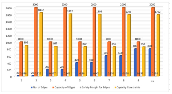
Figure 1. Safety margin and capacity constraints for edges.

In our simulation experiments, the number of nodes ranges from 5 to 40, while the number of edges ranges from 7 through 62. The actual graph (network topology) is chosen randomly. An example is shown in Figure 2. For each number of edges we ran the simulation with two different edge capacities: $C=1000$ and $C=2000$ units. As the safety margin increases with higher capacities, the network can be better utilized, since the safety margin determines what percentage of the maximum capacity is utilized.

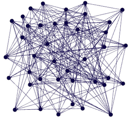
Figure 2. A sample network topology.

We ran the simulation with two different traffic types (two commodities in the multicommodity flow); they represent two source-terminal pairs, which were chosen randomly. Furthermore, the number of nodes and edges were varied: the nodes between 5 and 40, the edges between 7 and 62. The results are shown in Table 3. The table contains that for various numbers of nodes and edges, how many iterations were needed to find the optimum, and what was the optimum objective function value in terms of total carried traffic. The same results are represented graphically in Figure 3. The results allowed us to make some observations:

Table 3. Simulation results.

No. of Nodes ${\displaystyle \mathit{n}}$	No. of Edges ${\displaystyle \mathit{m}}$	Solved in Iteration ${\displaystyle \mathit{r}}$	Optimal Objective
5	7	2	550 × ${\displaystyle {10}^3}$
10	15	1	1.100 × ${\displaystyle {10}^3}$
15	22	1	1.650 × ${\displaystyle {10}^3}$
20	30	4	2.200 × ${\displaystyle {10}^3}$
25	39	5	2.750 × ${\displaystyle {10}^3}$
30	46	5	3.300 × ${\displaystyle {10}^3}$
35	54	6	3.850 × ${\displaystyle {10}^3}$
40	62	8	4.400 × ${\displaystyle {10}^3}$

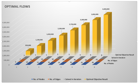
Figure 3. Optimal flows of packet traffic.

• As the number of nodes and edges increase, that is, the network becomes larger, the algorithm tends to require more iterations to find the optimum, which, of course, is not surprising.
• By setting the repetition parameter to $r=8$, the algorithm returned an optimal solution in 100% of the cases, which is very encouraging. It shows that one does not need an astronomical number of iterations to guarantee the optimum.
• In some cases (actually 25% the of all cases we tried) already the first iteration achieved the optimum. Furthermore, in 75% of cases at most 5 iterations were sufficient to reach the optimum, and we never needed more than 8. Of course, these are relatively small examples, but it reinforces the observation that a limited number of iterations suffice.

5. Conclusions

We have presented an efficient solution for the NP-complete Unsplittable Flow problem in directed graphs. The efficiency is achieved by sacrificing a small part of the solution space. The sacrificed part only contains scenarios where some edges are close to saturation, which is undesired in practical applications, anyway. The solutions that exclude such nearly saturated edges are called safe solutions.

The approach constitutes a new avenue to approximation, which we call safe approximation. It means that instead of giving up the exact solution, we rather restrict the search space to a (slightly) smaller one. When, however, the algorithm finds any solution, which happens with very high probability, then it is an exact (not just an approximate) solution.

References

- Karp, R.M. Reducibility Among Combinatorial Problems. In Complexity of Computer Computations; Miller, R.E., Thatcher, J.W., Eds.; Plenum Press: New York, NY, USA, 1972. [Google Scholar]
- Kramer, M.E.; van Leeuwen, J. The Complexity of Wire Routing and Finding the Minimum Area Layouts for Arbitrary VLSI Circuits. In Advances in Computing Research 2: VLSI Theory; Preparata, F., Ed.; JAI Press: London, UK, 1984. [Google Scholar]
- Middendorf, M.; Pfeiffer, F. On the Complexity of the Disjoint Paths Problem. In Polyhedral Combinatorics; Cook, W., Seymour, P.D., Eds.; DIMACS Series in Discrete Mathematics and Theoretical Computer Science; American Mathematical Society: Providence, RI, USA, 1990. [Google Scholar]
- Garg, N.; Vazirani, V.; Yannakakis, M. Primal-Dual Approximation Algorithms for Integral Flow and Multicuts in Trees, with Applications to Matching and Set Cover. In International Colloquium on Automata, Languages, and Programming; Springer: Berlin/Heidelberg, Germany, 1993; pp. 64–75. [Google Scholar]
- Faragó, A. Algorithmic Problems in Graph Theory. In Conference of Program Designers; Eötvös Loránd University of Sciences: Budapest, Hungary, 1985; pp. 61–66. [Google Scholar]
- Broder, A.A.; Frieze, A.M.; Suen, S.; Upfal, E. Optimal Construction of Edge-Disjoint Paths in Random Graphs. In Proceedings of the ACM-SIAM Symposium on Discrete Algorithms (SODA), Arlington, VA, USA, 23–25 January 1994; pp. 603–612. [Google Scholar]
- Robertson, N.; Seymour, P.D. Graph Minors-XIII: The Disjoint Paths Problem. J. Comb. 1995, 63, 65–110. [Google Scholar] [CrossRef]
- Bienstock, D.; Langston, M.A. Algorithmic implications of the Graph Minor Theorem. In Handbook in Operations Research and Management Science 7: Network Models; Ball, M.O., Magnanti, T.L., Monma, C.L., Nemhauser, G.L., Eds.; North-Hollandhl: Amsterdam, The Netherlands, 1995. [Google Scholar]
- Even, S.; Itai, A.; Shamir, A. On the complexity of timetable and multicommodity flow problems. SIAM J. Comput. 1976, 5, 691–703. [Google Scholar] [CrossRef]
- Aumann, Y.; Rabani, Y. Improved Bounds for All-Optical Routing. In Proceedings of the ACM-SIAM Symposium on Discrete Algorithms (SODA), San Francisco, CA, USA, 22–24 January 1995; pp. 567–576. [Google Scholar]
- Kleinberg, J.; Tardos, É. Approximations for the Disjoint Paths Problem in High-Diameter Planar Networks. In Proceedings of the ACM Symposium on Theory of Computing (STOC’95), Las Vegas, NV, USA, 29 May–1 June 1995; pp. 26–35. [Google Scholar]
- Guruswami, V.; Khanna, S.; Rajaraman, R.; Shepherd, B.; Yannakakis, M. Near-optimal hardness results and approximation algorithms for edge-disjoint paths and related problems. J. Comput. Syst. Sci. 2003, 67, 473–496. [Google Scholar] [CrossRef]
- Srinivasan, A. Improved Approximations for Edge-disjoint Paths, Unsplittable Flow, and Related Routing Problems. In Proceedings of the 38th IEEE Symposium on Foundations of Computer Science (FOCS’97), Miami Beach, FL, USA, 19–22 October 1997; pp. 416–425. [Google Scholar]
- Kolman, P.; Scheideler, C. Improved Bounds for the Unsplittable Flow Problem. J. Algorithms 2006, 61, 20–44. [Google Scholar] [CrossRef]
- Gonzales, T. (Ed.) Handbook of Approximation Algorithms and Metaheuristics; Chapman and Hall/CRC: Boca Raton, FL, USA, 2020. [Google Scholar]
- Raghavan, P. Probabilistic Construction of Deterministic Algorithms: Approximating Packing Integer Programs. J. Comput. Syst. Sci. 1988, 37, 130–143. [Google Scholar] [CrossRef]
Publisher’s Note: MDPI stays neutral with regard to jurisdictional claims in published maps and institutional affiliations. |
© 2021 by the authors. Licensee MDPI, Basel, Switzerland. This article is an open access article distributed under the terms and conditions of the Creative Commons Attribution (CC BY) license (http://creativecommons.org/licenses/by/4.0/).