Non-Overlapping LZ77 Factorization and LZ78 Substring Compression Queries with Suffix Trees

Abstract

We present algorithms computing the non-overlapping Lempel–Ziv-77 factorization and the longest previous non-overlapping factor table within small space in linear or near-linear time with the help of modern suffix tree representations fitting into limited space. With similar techniques, we show how to answer substring compression queries for the Lempel–Ziv-78 factorization with a possible logarithmic multiplicative slowdown depending on the used suffix tree representation.

1. Introduction

The Lempel–Ziv-77 (LZ77) [1] and Lempel–Ziv-78 (LZ78) [2] factorizations are some of the most well-studied techniques for lossless data compression. Several variants such as Lempel–Ziv–Storer–Szymanski (LZSS) [3] have been proposed, and nowadays we often perceive the LZSS factorization as the standard variant of the LZ77 factorization. Both are defined as follows: Given a factorization $T=F_1\cdots F_z$ for a string T:

• it is the LZSS factorization of T if each factor $F_x$, for $x\in \left[1..z\right]$, is either the leftmost occurrence of a character or the longest prefix of $F_x\cdots F_z$ that occurs at least twice in $F_1\cdots F_x$; or
• it is the classic LZ77 factorization of T if each factor $F_x$, for $x\in [1..z-1]$, is the shortest prefix of $F_x\cdots F_z$ that has only one occurrence in $F_1\cdots F_x$ (as a suffix). The last factor $F_z$ is the suffix $T[1+|F_1\cdots F_{z-1}|..]$ that may have multiple occurrences in $F_1\cdots F_z$.

The non-overlapping variation is to restrict, when computing $F_x$, all candidate occurrences of $F_x$ to end before $F_x$ starts. For LZSS, this means that a factor $F_x$ must occur at least once in $F_1\cdots F_{x-1}$. Given a text T of length n whose characters are drawn from an integer alphabet of size $\sigma =n^{\mathcal{O}\left(1\right)}$, we want to study the problem of computing the non-overlapping LZSS factorization memory-efficiently with the aid of two suffix tree representations, which were used by Fischer et al. [4] (Section 2.2) to compute the classic LZ77, LZSS, and LZ78 factorizations in linear time within the asymptotic space requirements of the respective suffix tree. In this article, we obtain the non-overlapping LZSS factorization with similar techniques and within the same space boundaries:

Theorem 1.

Given a text $T\left[1..n\right]$ of length n whose characters are drawn from an integer alphabet with size $\sigma =n^{\mathcal{O}\left(1\right)}$, we can compute its non-overlapping LZSS factorization

• in $\mathcal{O}\left({ϵ}^{-1}n\right)$ time using $(1+ϵ)nlgn+\mathcal{O}\left(n\right)$ bits (excluding the read-only text T); or
• in $\mathcal{O}\left(n{lg}^{ϵ}n\right)$ time using $\mathcal{O}(nlg\sigma )$ bits,

for a selectable constant $ϵ\in (0,1]$. We support outputting the factors directly or storing the factors within the (asymptotic) bounds of the working space such that we can retrieve a factor in constant time.

We also show that we can compute the longest previous non-overlapping factor table [5] within the same space and time complexities (Theorem 3) by providing a succinct representation of this table (Lemma 1).

Subsequently, we study the substring compression query problem [6], where the task is to compute the factorization of a given substring of the text in time related to the number of computed factors and possibly a logarithmic dependency on the text length. However, this problem has only been conceived for the LZ77 factorization family. Here, we provide the first non-trivial solutions for LZ78, again with the help of several suffix tree representations:

Theorem 2.

Given a text $T\left[1..n\right]$ of length n whose characters are drawn from an integer alphabet with size $\sigma =n^{\mathcal{O}\left(1\right)}$, we can compute a data structure on T in $\mathcal{O}\left(n\right)$ time that computes, given an interval $\mathcal{I}\subset \left[1..n\right]$, the LZ78 factorization of $T\left[\mathcal{I}\right]$ in

• $\mathcal{O}\left(z_{78\left[\mathcal{I}\right]}\right)$ time using $\mathcal{O}(nlgn)$ bits of space;
• $\mathcal{O}\left(z_{78\left[\mathcal{I}\right]}({log}_{\sigma }n+lg{z}_{78\left[\mathcal{I}\right]})\right)$ time using $\mathcal{O}(nlg\sigma )$ bits of space; or
• $\mathcal{O}({ϵ}^{-1}{z}_{78\left[\mathcal{I}\right]}lg{z}_{78\left[\mathcal{I}\right]})$ time using $(1+ϵ)nlgn+\mathcal{O}\left(n\right)$ bits of space,

where $z_{78\left[\mathcal{I}\right]}$ is the number of computed LZ78 factors and $ϵ\in (0,1]$ is a selectable constant. In the last result, we need additionally the $nlg\sigma$ bits of space for the read-only text during the queries if there is any character of the alphabet omitted in the text (otherwise, we can then simulate a text access with the function $\mathrm{head}$ as described in [4]).

We can further speed-up the last two solutions of Theorem 2 by spending more space (Theorem 4). Figure 1 shows a juxtaposition of all Lempel–Ziv factorizations addressed in this article.

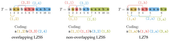
Figure 1. Juxtaposition of the overlapping LZSS factorization, the non-overlapping LZSS factorization, and the LZ78 factorization on the string $T=\mathtt{aaababaaaba}$. A factor is visualized by a rounded rectangle. Its coding consists of a mere character if it has no reference; otherwise, its coding consists of its referred position and its lengths for both LZSS variants or its referred index and its last character for LZ78.

2. Preliminaries

With lg we denote the logarithm ${log}_2$ to base two. Our computational model is the word RAM model with machine word size $\mathsf{\Omega }(lgn)$ for a given input size n. Accessing a word costs $\mathcal{O}\left(1\right)$ time.

Let T be a text of length n whose characters are drawn from an integer alphabet $\mathsf{\Sigma }=\left[1..\sigma \right]$ with $\sigma =n^{\mathcal{O}\left(1\right)}$. Given $X,Y,Z\in {\mathsf{\Sigma }}^{*}$ with $T=XYZ$, then X, Y, and Z are called a prefix, substring, and suffix of T, respectively. We call $T[i..]$ the ith suffix of T and denote a substring $T\left[i\right]\cdots T\left[j\right]$ with $T\left[i..j\right]$.

Given a character $\mathtt{c}\in \mathsf{\Sigma }$ and an integer j, the rank query $T.{rank}_{\mathtt{c}}\left(j\right)$ counts the occurrences of c in $T\left[1..j\right]$ and the select query $T.{select}_{\mathtt{c}}\left(j\right)$ gives the position of the jth c in T. We stipulate that ${rank}_{\mathtt{c}}\left(0\right)={select}_{\mathtt{c}}\left(0\right)=0$. If the alphabet is binary, i.e., when T is a bit vector, there are data structures [7,8] that use $o\left(\right|T\left|\right)$ extra bits of space and can compute ${rank}_{}$ and ${select}_{}$ in constant time, respectively. Each of those data structures can be constructed in time linear in $\left|T\right|$. We say that a bit vector has a rank-support and a select-support if it is endowed by data structures providing constant time access to ${rank}_{}$ and ${select}_{}$, respectively.

From now on, we assume that T ends with a special character $ smaller than all other characters appearing in T. Under this assumption, there is no suffix of T having another suffix of T as a prefix. The suffix trie of T is the trie of all suffixes of T. There is a one-to-one relationship between the suffix trie leaves and the suffixes of T. The suffix tree $\mathsf{ST}$ of T is the tree obtained by compacting the suffix trie of T. Similar to the suffix trie, the suffix tree has n leaves, but the number of internal nodes of the suffix tree is at most n because every $\mathsf{ST}$ node is branching. The string stored in a suffix tree edge e is called the label of e. We define the function $c\left(e\right)$ returning, for each edge e, the length of e’s label. The string label of a node v is defined as the concatenation of all edge labels on the path from the root to v; its string depth, denoted by $\mathrm{str}\_\mathrm{depth}\left(v\right)$, is the length of its string label. The leaf corresponding to the ith suffix $T[i..]$ is labeled with the suffix number $i\in \left[1..n\right]$. We write $\mathrm{sufnum}\left(\lambda \right)$ for the suffix number of a leaf $\lambda$. The leaf-rank is the preorder rank ($\in \left[1..n\right]$) of a leaf among the set of all $\mathsf{ST}$ leaves, denoted by $\mathrm{leaf}\_\mathrm{rank}\left(\lambda \right)$ for a leaf $\lambda$. For instance, the leftmost leaf in $\mathsf{ST}$ has leaf-rank 1, while the rightmost leaf has leaf-rank n. The function $\mathrm{next}\_\mathrm{leaf}\left(\lambda \right)$ returns the leaf whose suffix number is the suffix number of $\lambda$ incremented by one, or 1 if the suffix number of $\lambda$ is n.

Reading the suffix numbers stored in the leaves of $\mathsf{ST}$ in leaf-rank order gives the suffix array [9]. We denote the suffix array and the inverse suffix array of T by $\mathsf{SA}$ and $\mathsf{ISA}$, respectively. The array $\mathsf{ISA}$ is defined such that $\mathsf{ISA}\left[\mathsf{SA}\left[i\right]\right]=i$ for every $i=1,\dots ,n$. The two arrays $\mathsf{SA}$ and $\mathsf{ISA}$ have the following relation with the two operations $\mathrm{leaf}\_\mathrm{rank}$ and $\mathrm{sufnum}$ on the $\mathsf{ST}$ leaves:

• For the $\mathsf{ST}$ leaf $\lambda$ with $\mathrm{sufnum}\left(\lambda \right)=i$, we have $\mathrm{leaf}\_\mathrm{rank}\left(\lambda \right)=\mathsf{ISA}\left[i\right]$.
• For the $\mathsf{ST}$ leaf $\lambda$ with $\mathrm{leaf}\_\mathrm{rank}\left(\lambda \right)=j$, we have $\mathrm{sufnum}\left(\lambda \right)=\mathsf{SA}\left[j\right]$.

$\mathsf{LCP}\left[1..n\right]$ is an array with $\mathsf{LCP}\left[1\right]:=0$ and $\mathsf{LCP}\left[j\right]$ being the length of the longest common prefix (LCP) of the lexicographically jth smallest suffix $T\left[\mathsf{SA}\right[j]..]$ with its lexicographic predecessor $T\left[\mathsf{SA}\right[j-1]..]$ for $j\in \left[2..n\right]$. The permuted LCP array $\mathsf{PLCP}$ ([10] [Section 4]) is a permutation of $\mathsf{LCP}$ with $\mathsf{PLCP}\left[i\right]:=\mathsf{LCP}\left[\mathsf{ISA}\right[i\left]\right]$ for $i\in \left[1..n\right]$, and can be stored within $2n+o\left(n\right)$ bits of space. The $\mathsf{\Psi }$-function [11] is defined by $\mathsf{SA}\left[i\right]=\mathsf{SA}\left[\mathsf{\Psi }\right(i\left)\right]-1$ for $i\in \left[1..n\right]$ with $\mathsf{SA}\left[i\right]\ne n$ (and $\mathsf{\Psi }\left(i\right)=\mathsf{ISA}\left[1\right]$ for $\mathsf{SA}\left[i\right]=n$). It can be stored in $\mathcal{O}(nlg\sigma )$ bits while supporting constant access time [12].

In this article, we focus on the following two suffix tree representations, which are an ensemble of some of the aforementioned data structures:

• The succinct suffix tree (SST), using $(1+ϵ)nlgn+\mathcal{O}\left(n\right)$ bits of space ([4] [Section 2.2.3]) for a selectable constant $ϵ>0$, contains, among others, a $(1+ϵ)nlgn$-bits representation of $\mathsf{SA}$ and $\mathsf{ISA}$ with $\mathcal{O}(1/ϵ)$ access time for each array.
• The compressed suffix tree (CST) using $\mathcal{O}(nlg\sigma )$ bits of space [10,13] contains, among others, the $\mathsf{\Psi }$-function.

Both suffix tree representations can be constructed in linear time within their final space requirements (asymptotically) when neglecting the space requirements of the read-only text T. They store the $\mathsf{PLCP}$ array and a succinct representation of the suffix tree topology such as a balanced parentheses (BP) [7] sequence. The BP sequence represents a rooted, unlabeled but ordered tree of n nodes by a bit vector of length $2n+o\left(n\right)$ bits. Since the suffix tree has at most $2n$ nodes, the BP representation of the $\mathsf{ST}$ topology uses at most $4n+o\left(n\right)$ bits. For example, the BP sequence of the suffix tree given in Figure 2 is $\stackrel{1}{(}\stackrel{2}{\left(\right)}\stackrel{3}{(}\stackrel{4}{\left(\right)}\stackrel{5}{(}\stackrel{6}{\left(\right)}\stackrel{7}{\left(\right)}\stackrel{}{)}\stackrel{8}{(}\stackrel{9}{\left(\right)}\stackrel{10}{\left(\right)}\stackrel{}{)}\stackrel{}{)}\stackrel{11}{(}\stackrel{12}{\left(\right)}\stackrel{13}{\left(\right)}\stackrel{}{)}\stackrel{}{)}$, where we label the starting of an internal node and the center of a leaf ‘()’ with the respective preorder number on top. The BP sequence can be conceptionally constructed by performing a preorder traversal on the tree, writing an opening parenthesis when walking down an edge and writing a closing parenthesis when climbing up an edge. We augment the BP sequence of $\mathsf{ST}$ with auxiliary data structures [14] of $o\left(n\right)$ bits to support queries such as $\mathrm{parent}\left(v\right)$ returning the parent of a node v, a level ancestor query $\mathrm{level}\_\mathrm{anc}(\lambda ,d)$ returning the ancestor on depth d of the leaf $\lambda$, or $\mathrm{leaf}\_\mathrm{rank}\left(\lambda \right)$, all in constant time. Note that the depth of a node v, i.e., the number of edges from v to the root, is at most $\mathrm{str}\_\mathrm{depth}\left(v\right)$.

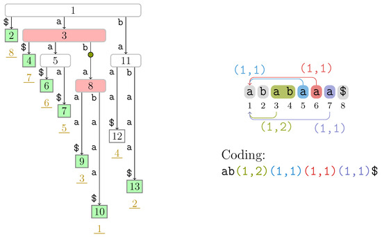
Figure 2. (Left) Suffix tree of the text $T=\mathtt{ababaaa}\$$ with the witness nodes and the corresponding leaves of the non-overlapping LZSS factorization highlight in red () and in green (), respectively. We additionally mark the string ab with an implicit node () whose string label is equal to the factor with Type 3. The nodes are labeled by their preorder numbers. The suffix number of each leaf $\lambda$ is the underlined number drawn in dark yellow below $\lambda$. (Right) Non-overlapping LZSS factorization of T.

For our algorithms, we want to simulate a linear scan on the text from its beginning to its end by visiting the leaves in ascending order with respect to their suffix numbers (starting with the leaf with suffix number 1, and ending at the leaf with suffix number n). For that, we iteratively call $\mathrm{next}\_\mathrm{leaf}$. We can compute $\mathrm{next}\_\mathrm{leaf}$ by first computing the leaf-rank of the succeeding leaf $\mathrm{next}\_\mathrm{leaf}\left(\lambda \right)$ of a leaf $\lambda$ with $\mathrm{leaf}\_\mathrm{rank}\left(\mathrm{next}\_\mathrm{leaf}\left(\lambda \right)\right)=\mathsf{\Psi }\left[\mathrm{leaf}\_\mathrm{rank}\left(\lambda \right)\right]$, and then selecting $\mathrm{next}\_\mathrm{leaf}\left(\lambda \right)$ by its leaf-rank; we can select a leaf by its leaf-rank in constant time due to the BP sequence representation of the suffix tree topology (the BP sequence can be augmented with a rank- and select-support for leaves represented by the empty parentheses ‘()’). Since we can simulate $\mathsf{\Psi }$ with $\mathsf{SA}$ and $\mathsf{ISA}$, the SST needs $\mathcal{O}(1/ϵ)$ time for evaluating $\mathrm{next}\_\mathrm{leaf}$.

Finally, a factorization of T of size z partitions T into z substrings $F_1\cdots F_z=T$. Each such substring $F_x$ is called a factor. In what follows, we deal with the non-overlapping LZSS factorization in Section 3, and subsequently (in Section 4) with the LZ78 factorization in the special context that we want to compute it on a substring of T after a preprocessing step.

3. Non-Overlapping LZSS

Let $z_{\mathrm{ov}}$ and z denote the number of factors of the overlapping LZSS factorization (i.e., the standard LZSS factorization supporting overlaps) and of the non-overlapping LZSS factorization, respectively. Kosolobov and Shur [15] showed that $z_{\mathrm{ov}}\le z\le z_{\mathrm{ov}}·\mathcal{O}(lg(n/($$z_{\mathrm{ov}}{log}_{\sigma }{z}_{\mathrm{ov}}\left)\right))$. Although being inferior to the overlapping LZSS factorization with respect to the number of factors, the non-overlapping LZSS factorization is an important tool for finding approximate repetitions [16], periods [17], seeds [18], tandem repeats [19], and other regular structures (cf. the non-overlapping s-factorization in ([20] [Chpt. 8])).

Algorithms computing the non-overlapping LZSS factorization usually compute the longest previous non-overlapping factor table $\mathsf{LPnF}\left[1..n\right]$, where $\mathsf{LPnF}\left[i\right]$ stores the length of the LCP of $T[i..]$ with all substrings $T[j..i-1]$ for $j\in [1..i-1]$, which we set to zero if no such substring exists (i.e., $\mathsf{LPnF}\left[1\right]=0$). Having $\mathsf{LPnF}$, we can iteratively compute the non-overlapping LZSS factorization because $F_x=T[k_x..k_x+max(0,\mathsf{LPnF}\left[k_x\right]-1)]$ with $k_x:={\sum }_{y=1}^{x-1}\left|F_y\right|+1$ for $x\in \left[1..z\right]$.

We are aware of the algorithms of Crochemore and Tischler [5] and Crochemore et al. [21] computing $\mathsf{LPnF}$ in linear time with a linear number of words. There are further practical optimizations [22,23,24] computing $\mathsf{LPnF}$ in linear time for constant alphabets. Finally, Ohlebusch and Weber [25] gave a linear time conversion algorithm from the longest previous factor table $\mathsf{LPF}$ [26] to $\mathsf{LPnF}$ if the leftmost possible referred positions $P\left[1..n\right]$ with $T\left[P\right[i\left]..P\right[i]+\mathsf{LPF}[i]-1]=T[i..i+\mathsf{LPF}[i]-1]$ for each text position $i\in \left[1..n\right]$ are provided. It seems possible that, instead of overwriting the $\mathsf{LPF}$ array with the $\mathsf{LPnF}$ array, we could run their algorithm on a $2n$-bits succinct representation of the $\mathsf{LPF}$ array supporting sequential scan in constant time ([27] [Corollary 5]) to produce an $\mathsf{LPnF}$ array representation within the same space due to the following lemma:

Lemma 1.

$\mathsf{LPnF}[j-1]-1\le \mathsf{LPnF}\left[j\right]\le n-j$ for $j\in \left[2..n\right]$.

Proof. 

Assume that $\mathsf{LPnF}[j-1]>0$ (since $\mathsf{LPnF}\left[j\right]\ge 0$ trivially holds). According to the definition, there exists an occurrence $T[i..i+\mathsf{LPnF}[j-1]-1]$ of $T[j-1..j-1+\mathsf{LPnF}[j-1]-1]$ with $i+\mathsf{LPnF}[j-1]-1<j-1$. Hence, $T[i+1..i+\mathsf{LPnF}[j-1]-1]=T[j..j+\mathsf{LPnF}[j-1]-2]$ and $\left|T\right[j..j+\mathsf{LPnF}[j-1]-2\left]\right|=\mathsf{LPnF}[j-1]-1$. Thus, $T[j..]$ has a common prefix with a substring of $T[1..j-1]$ of (at least) length $\mathsf{LPnF}[j-1]-1$, i.e., $\mathsf{LPnF}[j-1]-1\le \mathsf{LPnF}\left[j\right]$. The upper bound follows from the fact that a factor cannot protrude T to the right. □

Consequently, $\mathsf{LPnF}\left[1\right]+1,\mathsf{LPnF}\left[2\right]+2,\dots ,\mathsf{LPnF}\left[n\right]+n$ is non-decreasing. By storing the differences $\mathsf{LPnF}\left[j\right]-\mathsf{LPnF}[j-1]+1\ge 0$ for $j\in \left[2..n\right]$ in a unary bit sequence, we can linearly decode $\mathsf{LPnF}$ from this unary bit sequence because we know that $\mathsf{LPnF}\left[1\right]=0$. Since $\mathsf{LPnF}\left[n\right]+n\le n$ by the above lemma (in particular $\mathsf{LPnF}\left[i\right]\le \mathsf{LPF}\left[i\right]$), the sequence has at most $2n$ bits. Obviously, this sequence can be written sequentially from right to left in constant time per $\mathsf{LPnF}$ value in reverse order $\mathsf{LPnF}\left[n\right],\dots ,\mathsf{LPnF}\left[1\right]$ (the algorithm of Ohlebusch and Weber [25] computes $\mathsf{LPnF}$ in this order). It is therefore possible to compute $\mathsf{LPnF}$ within $\mathcal{O}\left(n\right)$ bits on top of P and a compressed indexing data structures such as the FM-index [28] of the text: For that purpose, Okanohara and Sadakane [29] proposed an algorithm computing $\mathsf{LPF}$ and P with the FM-index in $\mathcal{O}\left(n{lg}^{3}n\right)$ time, which was improved by Prezza and Rosone [30] to $\mathcal{O}\left(n{lg}^{2}n\right)$ time. However, the need of P, using $nlgn$ bits when stored in a plain array, makes an approach that transforms $\mathsf{LPF}$ to $\mathsf{LPnF}$ after computing $\mathsf{LPF}$ and P rather unattractive. In what follows, we present a different way that directly computes the non-overlapping LZSS factorization or $\mathsf{LPnF}$ with near-linear or linear running time, without the need of P.

3.1. Setup

Our idea is an adaptation of the LZSS factorization introduced in ([4] [Section 3]). To explain our approach, we first stipulate that T ends with a unique character $ that is smaller than all other characters appearing in T. Next, we distinguish between fresh and referencing factors. We say that a factor is fresh if it is the leftmost occurrence of a character. We call all other factors referencing. A referencing factor $F_x$ has a reference pointing to the starting position of its longest previous occurrence (as a tie break, we always select the leftmost such position). We call this starting position the referred position of $F_x$. More precisely, the referred position of a factor $F_x=T[i..i+\ell -1]$ is the smallest text position j with $j+\ell \le i$ and $T[j..j+\ell -1]=T[i..i+\ell -1]$. Compared to the overlapping LZSS factorization, we require here the additional restriction that $j+\ell \le i$. This makes the computation of the referred positions more technical: Let j be the referred position of a factor $F:=T[i..i+\ell -1]$, and let S be the longest substring starting before i that is a prefix of $T[i..]$. We associate the factor F with one of the following three types:

Type 1:

$T[j..j+\ell -1]=S$ (the factor F coincides with the overlapping LZSS factor that would start at $T[i..]$);

Type 2:

$T[j..j+\ell -1]$ is shorter than S, but $T[j+\ell ]\ne T[i+\ell ]$ (then there is a suffix tree node that has the string label F); or

Type 3:

$T[j+\ell ]=T[i+\ell ]$ and $j+\ell =i$ (otherwise, the factor F could be extended to the right).

An example is $T=\mathrm{a}|\mathrm{b}|\stackrel{3}{\mathrm{ab}}|\stackrel{1}{\mathrm{a}}|\stackrel{2}{\mathrm{a}}|\stackrel{1}{\mathrm{a}}|\$$, where the factor borders are symbolized by the vertical bar ∣, and the referencing factors are labeled with their types (fresh factors are not labeled). If F is of Type 3, the suffixes $T[j..]$ and $T[i..]$ share more than ℓ characters such that F is not a string label of any suffix tree node in general, but it is at least a prefix of the string label of a node. This is the case for the third factor ab in the aforementioned example, as can be seen in Figure 2.

To find the referred positions, we mark certain nodes as witnesses, which create a connection between corresponding leaves and their referred positions. A leaf is called corresponding if its suffix number is the starting position of a factor. We say that the witness of a fresh factor is the root. For a referencing factor F, the witness of F is the highest node whose string label has F as a prefix; the witness of F determines the referred position of F, which is the smallest suffix number among all leaves in its subtree.

Despite this increased complexity compared to the overlapping LZSS factorization, the non-overlapping factorization can be computed with the suffix tree in $\mathcal{O}(nlg\sigma )$ time using $\mathcal{O}(nlgn)$ bits of space ([31] [APL16]). Here, we adapt the algorithms of (Fischer et al. [4] [Section 3]) computing the overlapping LZSS factorization to compute the non-overlapping factorization by following the approach of Gusfield [31]. Our goal is to compute the coding of the factors, i.e., the referred position and the length of each factor (cf. Figure 1).

3.2. The Factorization Algorithm

All LZSS factorization algorithms of (Fischer et al. [4] [Section 3]) are divided into passes. A pass consists of visiting suffix tree leaves in text order (i.e., in order of their suffix numbers). On visiting a leaf, they conduct a leaf-to-root traversal. In what follows, we present our modification, which merely consists of a modification of Pass (a) in all LZSS factorization variants of ([4] [Section 3]): In Pass (a), Fischer et al. computed the factor lengths and the witnesses. To maintain the witnesses and lengths in future passes, they marked and stored the preorder numbers of the witnesses and the starting positions of the LZSS factors in two bit vectors $B_W$ and $B_T$, respectively. In succeeding passes, they computed, based on the factor lengths and the witnesses, the referred positions and with that the final coding. Therefore, it suffices to only change Pass (a) according to our definition of witnesses and factors, while keeping the subsequent passes untouched. In this pass, we do the following:

Pass (a)

Create $B_W$ and $B_T$ to determine the witnesses and the factor lengths, respectively.

The main technique of a pass in [4] are leaf-to-root traversals. Here, we do the opposite: We traverse from the root to a specific leaf. We perform a root-to-leaf traversal by level ancestor queries such that visiting a node takes constant time. We perform these traversals only for all corresponding leaves since the other leaves are not useful for determining a factor.

Suppose we visit a leaf $\lambda$ corresponding to a factor F. We already know the starting position of F (i.e., $\mathrm{sufnum}\left(\lambda \right)$), but not its length, referred position, or witness w. To detect w, we use the following observation: Given $j_u$ is the smallest suffix number among all leaves in the subtree rooted at a node u, w is the highest node that maximizes

$${\ell }_w:=min(\mathrm{str}\_\mathrm{depth}\left(w\right),\mathrm{sufnum}\left(\lambda \right)-j_w).$$

(1)

If $j_w=\mathrm{sufnum}\left(\lambda \right)$, then F is a fresh factor. Otherwise, w determines the length $\left|F\right|={\ell }_w$ and the referred position $j_w$ of F. However, the two functions $v\mapsto \mathrm{str}\_\mathrm{depth}\left(v\right)$ and $v\mapsto \mathrm{sufnum}\left(\lambda \right)-j_v$ are strictly increasing and monotonically decreasing, respectively, when applied to each node v visited when walking downwards the path from the root to $\lambda$. Thus, our goal is to find the lowest node u, where the value ${\ell }_u$ of Equation (1) still results from $\mathrm{str}\_\mathrm{depth}\left(u\right)$, and not from the second argument $\mathrm{sufnum}\left(\lambda \right)-j_u$. We give a sketch in Figure 3 and study a particular case in Figure 4 for factors of Types 2 and 3.

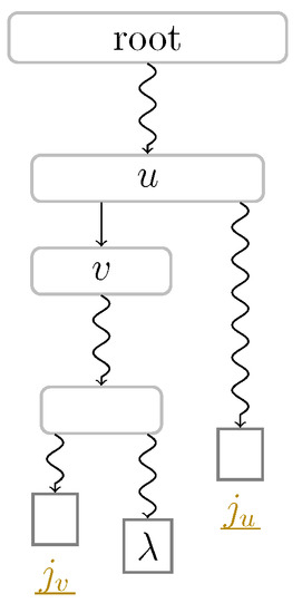
Figure 3. Determining the witness of a factor F whose starting position is the suffix number of the leaf $\lambda$. Straight arcs symbolize edges, while curly arcs symbolize paths that can visit multiple nodes (which are not visualized). Given $j_w$ is the smallest suffix number among all leaves in the subtree rooted at a node w, and that u is the lowest ancestor of $\lambda$ with $[j_u..j_u+\mathrm{str}\_\mathrm{depth}\left(u\right)-1]\cap [\mathrm{sufnum}\left(\lambda \right)..\mathrm{sufnum}\left(\lambda \right)+\mathrm{str}\_\mathrm{depth}\left(u\right)-1]=\varnothing$, then either u or its child v is the witness of F (see Section 3.2 for an explanation). The idea behind detecting whether the two intervals are intersecting is that a factor starting at $\mathrm{sufnum}\left(\lambda \right)$ of length $\mathrm{str}\_\mathrm{depth}\left(u\right)$ would be of Type 1 or Type 2 with referred position $j_u$. In fact, if F is of Type 1, then its witness is the lowest ancestor of $\lambda$ having a leaf with a suffix number smaller than $\mathrm{sufnum}\left(\lambda \right)$ in its subtree (this definition coincides with the witnesses of the overlapping LZSS factorization of ([4] [Section 2.3])). It is possible that $j_u=j_v$, i.e., the leaf with suffix number $j_u$ is also in the subtree rooted at v. We can observe this case in Figure 4.

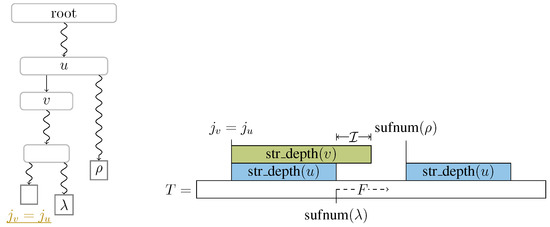
Figure 4. Special case of the setting considered in Figure 3 for factors of Types 2 and 3. Here, we assign u and v the same roles as in Figure 3, but we additionally assume that $j_v=j_u$ and $\mathrm{sufnum}\left(\lambda \right)\in \mathcal{I}:=[j_u+\mathrm{str}\_\mathrm{depth}\left(u\right)..j_u+\mathrm{str}\_\mathrm{depth}\left(v\right)-1]$. If $\mathrm{sufnum}\left(\lambda \right)=j_u+\mathrm{str}\_\mathrm{depth}\left(u\right)$, as in the right figure, then the factor F of $\lambda$ starting at $\mathrm{sufnum}\left(\lambda \right)$ is of Type 2, and the witness of F is u, although u is not the lowest ancestor of $\lambda$ having $\lambda$ and $j_u$ in its subtree. If $\mathrm{sufnum}\left(\lambda \right)\in \mathcal{I}\setminus \{j_u+\mathrm{str}\_\mathrm{depth}\left(u\right)\}$, then F is of Type 3 and the witness of F is v; the witness of F is v even if $\lambda$ and the leaf with suffix number $j_v$ are shared by a descendant of v as shown in the left figure.

To achieve our goal, let ${\mathcal{I}}_v:=[j_v..j_v+\mathrm{str}\_\mathrm{depth}\left(v\right)-1]$ and ${\mathcal{I}}_{\lambda ,v}:=[\mathrm{sufnum}\left(\lambda \right)..\mathrm{sufnum}\left(\lambda \right)+\mathrm{str}\_\mathrm{depth}\left(v\right)-1]$ be two intervals. These two intervals have the property that $T\left[{\mathcal{I}}_v\right]=T\left[{\mathcal{I}}_{\lambda ,v}\right]$. The idea is that $T\left[{\mathcal{I}}_{\lambda ,v}\right]$ is a candidate for F with $T\left[{\mathcal{I}}_v\right]$ being its leftmost occurrence in T. We compute the values of $j_v$, ${\mathcal{I}}_v$ and ${\mathcal{I}}_{\lambda ,v}$ for every node v on the path from the root to $\lambda$ until reaching a node v such that the intervals ${\mathcal{I}}_v$ and ${\mathcal{I}}_{\lambda ,v}$ overlap (cf. Line 9 in Algorithm 1). Let u be the parent of v. Then, the edge $(u,v)$ determines the factor F: We consider the following two cases that determine whether F is a fresh or referencing factor, and whether the witness and the referred position of F are u and $j_u$, or v and $j_v$, respectively, in case F is a referencing factor:

• If $j_v=\mathrm{sufnum}\left(\lambda \right)$, there is no leaf in v’s subtree with a suffix number smaller than $\mathrm{sufnum}\left(\lambda \right)$.

  -

  If u is the root, then there is no candidate for a referred position available, i.e., F is a fresh factor (cf. Line 13 in Algorithm 1).

  -

  Otherwise, $\mathrm{str}\_\mathrm{depth}\left(u\right)>0$ and ${\mathcal{I}}_u\cap {\mathcal{I}}_{\lambda ,u}=\varnothing$ (since v is the highest node on the path from the root to $\lambda$ for which ${\mathcal{I}}_v\cap {\mathcal{I}}_{\lambda ,v}\ne \varnothing$ holds). Hence, the longest substring occurring before $\mathrm{sufnum}\left(\lambda \right)$ that is a prefix of $T\left[\mathrm{sufnum}\right(\lambda )..]$ has an occurrence in $T\left[1..\mathrm{sufnum}\right(\lambda )-1]$ (Type 1). One of those occurrences starts at position $j_u$. This means that the referred position is $j_u$, and the witness of F is u; the length of F is $\mathrm{str}\_\mathrm{depth}\left(u\right)$ (cf. Line 17 in Algorithm 1).

• If $j_v\ne \mathrm{sufnum}\left(\lambda \right)$ (i.e., $j_v<\mathrm{sufnum}\left(\lambda \right)$), the length of F is in the interval $\left[\mathrm{str}\_\mathrm{depth}\right(u\left)..\mathrm{str}\_\mathrm{depth}\right(v)-1]$. If the factor F refers to the position $j_v$, then its length is the minimum of $\mathrm{sufnum}\left(\lambda \right)-j_v$ and the length of the LCP of the suffixes starting at $j_v$ and $\mathrm{sufnum}\left(\lambda \right)$. (Note that this LCP can be longer than the string label of v.) Let us denote the value of this minimum by ℓ, which coincides with ${\ell }_v$ of Equation (1) due to $\mathrm{str}\_\mathrm{depth}\left(v\right)\ge \mathrm{sufnum}\left(\lambda \right)-j_v$, and determines whether F refers to $j_v$ or $j_u$ (cf. Line 20 in Algorithm 1):

  -

  If $\ell =\mathrm{str}\_\mathrm{depth}\left(u\right)$, then the referred position of F is actually the suffix number of a leaf contained in u’s subtree (Type 2). In this case, the length of F is $\left|{\mathcal{I}}_u\right|=\mathrm{str}\_\mathrm{depth}\left(u\right)$ because ${\mathcal{I}}_u\cap {\mathcal{I}}_{\lambda ,u}=\varnothing$. The witness of F is u, and $j_u$ is the referred position (cf. Line 21 in Algorithm 1).

  -

  Otherwise, $\mathrm{str}\_\mathrm{depth}\left(u\right)<\left|F\right|<\mathrm{str}\_\mathrm{depth}\left(v\right)$, hence F is not the string label of any suffix tree node (Type 3). The node v is the highest node whose string label has F as a prefix. We conclude that the witness, referred position, and length of F are v, $j_v$, and ℓ, respectively (cf. Line 23 in Algorithm 1).

3.3. Complexity Bounds

To determine the value of $j_v$, we need to answer a range minimum query (RMQ) on $\mathsf{SA}$. Given an array $A\left[1..n\right]$, an RMQ for an interval $\mathcal{I}\subset \left[1..n\right]$ asks for the index of the minimum value in $A\left[\mathcal{I}\right]$. To answer an $\mathsf{RMQ}$, we can make use of the following data structure:

Lemma 2

([32] [Thm 5.8]). Let $A\left[1..n\right]$ be an integer array, where accessing an element $A\left[i\right]$ takes $t_A$ time for $i\in \left[1..n\right]$. There exists a data structure of size $2n+o\left(n\right)$ bits built on top of A that answers RMQs in constant time. It is constructed in $\mathcal{O}\left(t_{A}n\right)$ time with $o\left(n\right)$ additional bits of working space.

According to Lemma 2, we can construct an RMQ data structure in $\mathcal{O}\left(t_{\mathsf{SA}}n\right)$ time using $2n+o\left(n\right)$ bits of space, where $t_{\mathsf{SA}}$ is the time for accessing $\mathsf{SA}$. We can access $\mathsf{SA}$ in $\mathcal{O}(1/ϵ)$ time and in $\mathcal{O}\left({lg}^{ϵ}n\right)$ time with the SST and CST, respectively, where the last time complexity is due to the following lemma:

Lemma 3

(Grossi and Vitter [11] [Section 3.2]). There is a data structure using $\mathcal{O}\left({ϵ}^{-1}n\right)$ bits that can access $\mathsf{SA}$ in $\mathcal{O}\left({lg}^{ϵ}n\right)$ time, where $ϵ\in (0,1]$ is a selectable constant.

As shown by (Fischer et al. [33] [Lemma 3]), the operation $\mathrm{str}\_\mathrm{depth}\left(u\right)$ for a node u can be computed with $\mathsf{SA}$, $\mathsf{LCP}$, and an RMQ data structure on $\mathsf{LCP}$ because the leaf-ranks of the leftmost leaf ${\lambda }_{\mathrm{L}}$ and rightmost leaf ${\lambda }_{\mathrm{R}}$ in the subtree rooted u define the interval $[\mathrm{leaf}\_\mathrm{rank}\left({\lambda }_{\mathrm{L}}\right)+1..\mathrm{leaf}\_\mathrm{rank}\left({\lambda }_{\mathrm{R}}\right)]$ in $\mathsf{SA}$, and selecting the minimum value in $\mathsf{LCP}$ within this interval gives the length of the longest common prefix shared among all leaves in u’s subtree, which is $\mathrm{str}\_\mathrm{depth}\left(u\right)$. However, we do not store $\mathsf{LCP}$ explicitly, but instead simulate an access of its jth entry for $j\in \left[2..n\right]$ by $\mathsf{LCP}\left[j\right]=\mathsf{PLCP}\left[\mathsf{SA}\right[j\left]\right]$. Hence, we can access an entry of $\mathsf{LCP}$ in $\mathcal{O}\left(t_{\mathsf{SA}}\right)$ time. Consequently, we can build the data structure of Lemma 2 on $\mathsf{LCP}$ in $\mathcal{O}\left(t_{\mathsf{SA}}n\right)$ time, which takes $2n+o\left(n\right)$ bits of additional space. Equipped with this data structure, we finally can evaluate $\mathrm{str}\_\mathrm{depth}$ in $\mathcal{O}\left(t_{\mathsf{SA}}\right)$ time. The total time bounds are composed as follows:

(a)

Since the number of visited nodes is at most the factor length of a corresponding leaf $\lambda$ during a root-to-leaf traversal to $\lambda$, and ${\sum }_{x=1}^z\left|F_x\right|=n$, we conclude that the RMQs take $\mathcal{O}\left(n{t}_{\mathsf{SA}}\right)$ time in total.

(b)

For each root-to-leaf traversal to a leaf corresponding to a factor F, we stop at an edge $(u,v)$ and compute the length of the LCP of $T[j_v..]$ and $T\left[\mathrm{sufnum}\right(\lambda )..]$ by naïvely comparing $\mathcal{O}\left(\left|F\right|\right)$ characters. In total, the number of compared characters is $\mathcal{O}\left({\sum }_{x=1}^z\left|F_x\right|\right)=\mathcal{O}\left(n\right)$.

Altogether, Pass (a) takes takes $\mathcal{O}\left(n{t}_{\mathsf{SA}}\right)$ time, since all applied tree navigational operations take constant time. With Lemma 3, we obtain the time and space complexities claimed in Theorem 1.

Algorithm 1: Pass (a) of the non-overlapping LZSS algorithm of Section 3. The function $\mathrm{report}(w,j,\ell )$ outputs the referred position j and the length ℓ of the respective referencing factor; marks the witness w and the starting position of the next factor (determined by ℓ) in $B_W$ and in $B_T$, respectively; and appends the unary value of $\mathrm{depth}\left(w\right)$ to $B_L$ (defined in Section 3.4). $\mathrm{lmost}\_\mathrm{leaf}\left(v\right)$ and $\mathrm{rmost}\_\mathrm{leaf}\left(v\right)$ return the leftmost and the rightmost leaf of the subtree rooted at v in constant time, respectively. All break statements exit the nested inner loop and jump to Line 25.

3.4. Storing the Factorization

From here on, we have two options: We can either directly output the referred positions and the lengths of the computed factors during Pass (a), or we can store additional information for retrieving the witnesses in a later pass. Such a later pass is interesting when working with the SST, as we can store the factors in the $(1+ϵ)nlgn+\mathcal{O}\left(n\right)$ bits of working space ([4] [Section 3.3]). There, a later pass overwrites the space occupied by the SST, in particular the suffix array representation, such that later passes no longer can determine witnesses. Although we mark each witness in the bit vector $B_W$ during Pass (a), there can be multiple nodes marked in $B_W$ on the path from the root to a leaf corresponding to a factor F. The overlapping LZSS factorization obeys the invariant that the witness of F is the lowest ancestor of $\lambda$ that is marked in $B_V$, given that $B_V$ marks all ancestors of the leaves with a suffix number smaller than $\mathrm{sufnum}\left(\lambda \right)$ when conducting a leaf-to-root traversal at $\lambda$ during the overlapping LZSS computation ([4] [Section 3]). Due to the existence of factors of Types 2 and 3, this invariant does not hold for the non-overlapping factorization.

For the later passes, we want a data structure that finds the witness w of a factor F based on F’s starting position in constant time. Fortunately, w is determined by the leaf $\lambda$ corresponding to F and w’s depth due to $w=\mathrm{level}\_\mathrm{anc}\left(\lambda ,\mathrm{depth}\left(w\right)\right)$. To remember the depth of each witness, we maintain a bit vector $B_L$ that stores the depth of each witness in unary coding sorted by the suffix number of the respective corresponding leaf. Given that we find the witness w of a leaf $\lambda$ in Pass (a) during the traversal from the root to $\lambda$, we store the unary code ${\mathtt{0}}^d\mathtt{1}$ in $B_L$, where $d:=\mathrm{depth}\left(w\right)$. For a leaf corresponding to a fresh factor, we store the unary code 1 in $B_L$. Similar to $B_D$ in ([4] [Sect. 3.4.3 Pass (2)]), we do not need to add a select-support to $B_L$, since we process the corresponding leaves always sequentially in text order. Given a corresponding leaf $\lambda$, we can jump to its witness (or to the root if $\lambda$ corresponds to a fresh factor) with a level ancestor query from $\lambda$ with the depth $B_L.{select}_1(\mathrm{sufnum}\left(\lambda \right)+1)-B_L.{select}_1(\mathrm{sufnum}\left(\lambda \right))-1$. The length of $B_L$ is at most $n+z$ since the depth of a witness is bounded by the length of its corresponding factor and the sum of all factor lengths is n.

3.5. Computing $\mathsf{LPnF}$

Finally, we can compute $\mathsf{LPnF}$ with the same algorithm by visiting all leaves (i.e., not only the corresponding ones). However, we no longer can charge the visited nodes during a root-to-leaf traversal with the length of a factor as in Section 3.3 (a). In fact, such an algorithm may visit $\mathcal{O}\left(n^2\right)$ nodes since ${\sum }_{i=1}^n\mathsf{LPnF}\left[i\right]=\mathcal{O}\left(n^2\right)$ (and this sum is $\mathsf{\Theta }\left(n^2\right)$ for the string $T=\mathtt{a}\cdots \mathtt{a}$). To reduce the number of nodes to visit, we can make use of Lemma 1: having $\mathsf{LPnF}[1..i-1]$ computed, we know that $\mathsf{LPnF}\left[i\right]\ge \mathsf{LPnF}[i-1]-1$; hence, it suffices to start the root-to-leaf traversal at the lowest node $\tilde{w}$ whose string depth is at most $\mathsf{LPnF}[i-1]-1$. We find this node $\tilde{w}$ by a suffix link. A suffix link connects a node with string label $S\in {\mathsf{\Sigma }}^{+}$ to the node with string label $S[2..]$ or to the root node if $S\in {\mathsf{\Sigma }}^1$. All nodes except the root have a suffix link. However, we do not store suffix links as pointers explicitly, but simulate them with the leaves since we can compute the suffix link of a leaf $\lambda$ with $\mathrm{next}\_\mathrm{leaf}\left(\lambda \right)$: Suppose that we have processed the leaf $\lambda$ with suffix number $i-1$ for computing $\mathsf{LPnF}[i-1]$. In what follows, we first assume that the computed factor starting at $i-1$ is not of Type 3. Then, the witness of $\lambda$ is $\lambda$’s ancestor u with $\mathrm{str}\_\mathrm{depth}\left(u\right)=\mathsf{LPnF}[i-1]$ being the computed factor length. First, we select another leaf ${\lambda }^{\prime }$ of the subtree rooted at u such that the lowest common ancestor (LCA) of $\lambda$ and ${\lambda }^{\prime }$ is u (e.g., we can select the leftmost or rightmost leaf in u’s subtree). Then, $\tilde{\lambda }:=\mathrm{next}\_\mathrm{leaf}\left(\lambda \right)$ is the leaf with suffix number i, and the LCA $\tilde{u}$ of $\tilde{\lambda }$ and $\mathrm{next}\_\mathrm{leaf}\left({\lambda }^{\prime }\right)$ is the node on the path from the root to $\tilde{\lambda }$ with $\mathrm{str}\_\mathrm{depth}\left(\tilde{u}\right)=\mathrm{str}\_\mathrm{depth}\left(u\right)-1$. By omitting the nodes from the root to $\tilde{u}$ in the traversal to $\tilde{\lambda }$ for computing $\mathsf{LPnF}\left[i\right]$, we only need to visit at most $\mathsf{LPnF}\left[i\right]-\mathsf{LPnF}[i-1]+1$ nodes for determining $\mathsf{LPnF}\left[i\right]$. A telescoping sum with the upper bound of Lemma 1 shows that we visit $\mathcal{O}\left(n\right)$ nodes in total.

It is left to deal with the text positions $i-1$ for which we computed a factor of Type 3. Here, the leaf $\lambda$ has a witness v with $\mathsf{LPnF}[i-1]<\mathrm{str}\_\mathrm{depth}\left(v\right)$, i.e., the computed factor is implicitly represented on the edge from $u:=\mathrm{parent}\left(v\right)$ to v. We apply the same technique (i.e., taking the suffix link) as for the other types, but apply this technique on u instead of the witness v, such that we end up at a node $\tilde{u}$ with $\mathrm{str}\_\mathrm{depth}\left(\tilde{u}\right)=\mathrm{str}\_\mathrm{depth}\left(u\right)-1$. We sketch the setting in Figure 5. Now, we additionally need to walk down from $\tilde{u}$ towards $\tilde{\lambda }=\mathrm{next}\_\mathrm{leaf}\left(\lambda \right)$ to reach the lowest node $\tilde{v}$ with $\mathrm{str}\_\mathrm{depth}\left(\tilde{v}\right)\le \mathsf{LPnF}[i-1]-1$. There can be at most $c(u,v)$ nodes on the path from $\tilde{u}$ to $\tilde{v}$. We can refine this number to at most $\delta :=\mathsf{LPnF}[i-1]-\mathrm{str}\_\mathrm{depth}\left(u\right)$, where $\delta$ is the number of characters on the edge $(u,v)$ contributing to $\mathsf{LPnF}[i-1]$. Nevertheless, these extra $\delta$ nodes seem to invalidate the $\mathcal{O}\left(n\right)$ bound on the number of visited nodes.

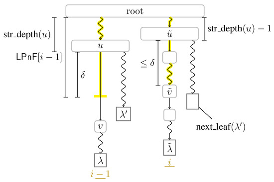
Figure 5. Computing $\mathsf{LPnF}\left[i\right]$ from $\mathsf{LPnF}[i-1]$ by simulating a suffix link from u to $\tilde{u}$ (cf. Section 3.5). Straight arcs symbolize edges, while curly arcs symbolize paths visiting multiple nodes (which are not visualized). We have $\mathrm{str}\_\mathrm{depth}\left(u\right)+\delta =\mathsf{LPnF}[i-1]$, and hence $\mathrm{str}\_\mathrm{depth}\left(\tilde{u}\right)+\delta =\mathsf{LPnF}[i-1]-1$. We have $\delta >0$ if and only if the factor starting at text position $i-1$ is of Type 3. In that case, we additionally walk down from $\tilde{u}$ towards $\tilde{\lambda }$ to find the lowest node $\tilde{v}$ with $\mathrm{str}\_\mathrm{depth}\left(\tilde{v}\right)\le \mathsf{LPnF}[i-1]-1=\mathrm{str}\_\mathrm{depth}\left(u\right)+\delta -1$. While u and v are directly connected with an edge, the path from $\tilde{u}$ to $\tilde{v}$ may contain multiple edges.

To retain our claimed time complexity, we switch from counting nodes to counting characters and use the following charging argument: We charge each edge we traversed by $c\left(e\right)$ characters, or ${\delta }_e$ characters if we only traversed ${\delta }_e\le c\left(e\right)$ characters on an edge. With the above analysis, we again obtain $\mathcal{O}\left(n{t}_{\mathsf{SA}}\right)$ time for the algorithm computing the non-overlapping factorization (as well as the non-Type 3 $\mathsf{LPnF}$ values) by spending $\mathcal{O}\left(t_{\mathsf{SA}}\right)$ time for each charged character (instead of each visited node).

Let us reconsider that the factor of $\mathsf{LPnF}[i-1]$ is of Type 3, where we charge the last edge $(u,v)$ for computing $\mathsf{LPnF}[i-1]$ with $\delta$ characters. Here, we observe that we actually spend only $\mathcal{O}\left(t_{\mathsf{SA}}\right)$ time for processing this edge. Hence, we have $\delta -1$ characters as a credit left, which we can spend on traversing $\mathcal{O}\left(\delta \right)$ descendants of $\tilde{u}$. If the factor starting at i is again of Type 3, we add the remaining credit to the newly gained credit, and recurse.

Regarding Section 3.3 (b), computing the length of the LCP of $T[j_v..]$ and $T\left[\mathrm{sufnum}\right(\lambda )..]$ naïvely results again in $\mathcal{O}\left(n^2\right)$ overall running time since we need to compute these lengths for all n positions. Here, instead of computing the length of such an LCP naïvely, we determine it by computing $\mathrm{str}\_\mathrm{depth}\left(w\right)$ of the LCA of $\lambda$ and the leaf ${\lambda }^{\prime }$ with suffix number $j_v$ in $\mathcal{O}\left(t_{\mathsf{SA}}\right)$ time. We find ${\lambda }^{\prime }$ with the RMQ data structure on $\mathsf{SA}$ that actually reports the leaf-rank instead of the suffix number $j_v$, which we obtain by accessing $\mathsf{SA}$. Altogether, we obtain the same time and space bounds for computing the non-overlapping LZSS factorization:

Theorem 3.

We can compute the $2n$-bits representation of $\mathsf{LPnF}$ within the same time and space as the non-overlapping LZSS factorization described in Theorem 1.

4. Substring Compression Query Problem

The substring compression query problem [6] is to find the compressed representation of $T\left[\mathcal{I}\right]$, given a query interval $\mathcal{I}\subset \left[1..n\right]$. Cormode and Muthukrishnan [6] solved this problem for LZSS with a data structure answering the query for $\mathcal{I}$ in $\mathcal{O}(z_{SS\left[\mathcal{I}\right]}lgnlglgn)$ time, where $z_{SS\left[\mathcal{I}\right]}$ denotes the number of produced LZSS factors of the queried substring $T\left[\mathcal{I}\right]$. Their data structure uses $\mathcal{O}\left(n{lg}^{ϵ}n\right)$ space, and it can be constructed in $\mathcal{O}(nlgn)$ time. This result was improved by Keller et al. [34] to $\mathcal{O}(z_{SS\left[\mathcal{I}\right]}lglgn)$ query time for the same space or to $\mathcal{O}\left(z_{SS\left[\mathcal{I}\right]}{lg}^{ϵ}n\right)$ query time for linear space. They also gave other trade-offs regarding query time and the size of the used data structure for larger data structures.

The main idea of tackling the problem for LZSS (and similarly for the classic LZ77 factorization) is to use a data structure answering interval LCP queries, which are usually answered by two-dimensional range successor/predecessor data structures. Most recently, Matsuda et al. [35] proposed a data structure answering an interval LCP query in $\mathcal{O}\left(n^{ϵ}\right)$ time while taking $\mathcal{O}\left({ϵ}^{-1}n(H_0\left(T\right)+1)\right)$ bits of space, where $H_0$ denotes the zeroth order empirical entropy. Therefore, they could implicitly answer a substring compression query in $\mathcal{O}\left(z_{SS\left[\mathcal{I}\right]}{n}^{ϵ}\right)$ time within compressed space. Recently, Bille et al. [36] proposed data structures storing the LZSS-compressed suffixes of T for answering a pattern matching query of an LZSS-compressed pattern P without decompressing P. Their proposed data structures also seem to be capable of answering substring compression queries.

As a warm up for the more-involving techniques for the LZ78 factorization below (cf. Section 4.5), we show that our techniques studied for the non-overlapping LZSS factorization in Section 3 can be adapted to the substring compression query problem under the restriction that the query interval starts at text position 1 (meaning that we query for prefixes instead of arbitrary substrings). Given an interval $\mathcal{I}=\left[1..p\right]$ for a text position $p\in \left[1..n\right]$, the algorithm of Theorem 1 achieves $\mathcal{O}\left(p{t}_{\mathsf{SA}}\right)$ time, where $t_{\mathsf{SA}}$ is the time to access $\mathsf{SA}$. We can improve the running time by replacing the linear scan on Line 10 of Algorithm 1 with an exponential search [37]: As long as the condition on Line 9 is true (the condition for walking downwards), we do not increment the depth d by one, but instead double d. Now, when the condition on Line 9 becomes false, we may have overestimated the desired depth (we want the first d for which the condition on Line 9 becomes false). Thus, we need to additionally backtrack by performing a binary search on the interval $[d/2..d]$. If we perform this search for computing a factor of length ℓ, then we double d at most $lg\ell$ times, and visit $\mathcal{O}(lg\ell )$ depths during the binary search (see also Figure 6 for a visualization). In total, we obtain $\mathcal{O}(z_{SS\left[1..p\right]}{t}_{\mathsf{SA}}lg\ell )$ time, where ℓ is the length of the longest non-overlapping LZSS factor (here, $z_{SS\left[1..p\right]}$ denotes the number of computed non-overlapping factors). Note that the result is not particularly interesting since we can just store the whole factorization of $T\left[1..n\right]$, scan for the leftmost factor $F_x$ that ends at p or after, trim $F_x$’s length to end at p, and finally return $F_1,\cdots ,F_x$, all in $\mathcal{O}\left(z_{SS\left[1..p\right]}\right)$ time.

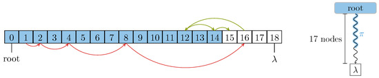
Figure 6. Exponential search on a root-to-leaf path for the first node that does not meet a specific condition. In the setting of the non-overlapping LZSS factorization of Section 4 as well as in the LZ78 factorization of Section 4.5, the path from the root to a leaf $\lambda$ contains a sub-path $\pi$ including the root whose contained nodes all share a common property (for LZSS they meet the condition on Line 10 of Algorithm 1, while for LZ78 they are edge witnesses marked in the bit vector $B_E$). We symbolize the path from the root to $\lambda$ as an array, where each node is represented by its depth. The sub-path $\pi$ is visualized by the shaded entries (). Here, the leaf $\lambda$ has depth 18, and we want to find the first unshaded node on depth 15. The exponential search and the subsequent binary search in the range $\left[8..16\right]$ is conducted by following the edges below and above the path array, respectively.

To generalize this algorithm for an interval $\mathcal{I}$ with $\mathsf{b}\left(\mathcal{I}\right)>1$, we need to change the definition of $j_v$ for a node v in Section 3.2 to be the smallest suffix number of at least $\mathsf{b}\left(\mathcal{I}\right)$ among the leaves in the subtree rooted at v. However, this additional complexity makes the approach selecting $j_v$ with an RMQ on $\mathsf{SA}$ infeasible and leads us back to the interval LCP query problem.

4.1. Related Substring Compression Query Problems

As far as the author is aware of, the substring compression query problem has only been studied for LZSS. However, Lifshits [38] mentioned that it is also feasible to think about the substring compression query problem in context of straight-line programs (SLPs): Given an SLP of size g representing T, we can construct an SLP of size $\mathcal{O}\left(g\right)$ on $T\left[\mathcal{I}\right]$ in $\mathcal{O}\left(g\right)$ time. Actually, we can do better if the SLP is locally consistent. For that, we augment each non-terminal with the number of terminal symbols it expands to (after recursively expanding all non-terminals by their right hand sides). For a grammar such as HSP ([39] [Theorem 3.5]), we can compute the SLP variant of HSP (analogously to the SLP variant of ESP [40]) in $\mathcal{O}(lg|\mathcal{I}|{lg}^{*}n)$ time, or ESP [41] in $\mathcal{O}({lg}^2\left|\mathcal{I}\right|{lg}^{*}n)$ time due to ([39] [Lemma 2.11]).

Here, we consider answering substring compression queries with the LZ78 factorization (which is actually also an SLP ([42] [Section VI.A.1])), i.e., the goal is to compress the substring $T\left[\mathcal{I}\right]$ with LZ78. Let $z_{78\left[\mathcal{I}\right]}$ denote the number of LZ78 factors of the string $T\left[\mathcal{I}\right]$. When the text is given as an SLP of size g, we can first transform this SLP into an SLP of $T\left[\mathcal{I}\right]$ in $\mathcal{O}\left(g\right)$ time, and then apply the algorithm of Bannai et al. [43] on this SLP to compute the LZ78 factorization in $\mathcal{O}(g+z_{78\left[\mathcal{I}\right]}lg{z}_{78\left[\mathcal{I}\right]})$ time. Let us consider from now on that T is given in its plain form as a string with $nlg\sigma$ bits. A possible way is to apply first a solution for computing an LZ77 substring compression query, and then transform the LZ77-compressed substring into an SLP of size $\mathcal{O}(z_{SS\left[\mathcal{I}\right]}lg\left|\mathcal{I}\right|)$ in $\mathcal{O}(z_{SS\left[\mathcal{I}\right]}lg\left|\mathcal{I}\right|)$ time by a transformation due to Rytter [44], to finally apply the aforementioned algorithm of Bannai et al. [43]. The fastest LZ78 factorization algorithms [4,45] can answer a LZ78 substring compression query in $\mathcal{O}\left(\right|\mathcal{I}\left|\right)$ time alphabet independently. For small alphabet sizes, the running time ${\mathcal{O}\left(\right|\mathcal{I}\left|\right(lglg\left|\mathcal{I}\right|)}^2/({log}_{\sigma }\left|\mathcal{I}\right|lglglg\left|\mathcal{I}\right|\left)\right)$ of the LZ78 factorization algorithm of Jansson et al. [46] becomes even sub-linear in $\left|\mathcal{I}\right|$. However, for large $\mathcal{I}$ and a compressible text T, these approaches are rather slow compared to the solutions for LZSS mentioned above, whose running times are bounded by the number of computed factors and a logarithmic multiplicative factor on the text length.

To obtain similar bounds for LZ78, we could adapt the approach of Bille et al. [36] to preprocess the LZ78 factorization of all suffixes of T, but that would give us a data structure with super-linear preprocessing time (and possibly super-linear space). Here, we borrow the idea from Nakashima et al. [45] to superimpose the suffix tree with the LZ78 trie, and use a data structure for answering nearest marked ancestor queries to find the lowest marked suffix tree node on the path from the root to a leaf. This data structure [47] takes $\mathcal{O}(nlgn)$ bits of space, and can answer a nearest marked ancestor query in $\mathcal{O}\left(1\right)$ amortized time. We are unaware whether there are improvements for this type of query, even under the light that they only need to answer fringe marked ancestor queries, a notion coined by Breslauer and Italiano [48], which is a special case of nearest marked ancestor queries: in the fringe marked ancestor query problem, the root of a tree (here: the suffix tree) is already marked, and we can only mark the children of an already marked node. In what follows, we formally define the LZ78 factorization, and then propose approaches for the LZ78 substring compression query problem based on different suffix tree representations.

4.2. LZ78 Factorization

Stipulating that $F_0$ is the empty string, a factorization $F_1\cdots F_z=T$ is called the LZ78 factorization [2] of T iff, for all $x\in \left[1..z\right]$, the factor $F_x$ is the longest prefix of $T\left[\right|F_1\cdots F_{x-1}|+1..]$ with $F_x=F_y\mathtt{c}$ for some $y\in [0..x-1]$ and $\mathtt{c}\in \mathsf{\Sigma }$, that is, $F_x$ is the longest possible previous factor $F_y$ appended by the following character $T\left[\right|F_1\cdots F_x\left|\right]$ in the text. We say that y is the referred index of the factor $F_x$. A factor is thus determined by its referred index and its last character, which lets us encode the factors in a list of (integer, character)-pairs, as shown in the example of Figure 1 where we simplify the coding of factors with referred index 0 to plain characters (to ease the comparison with the LZSS variants). Figure 7 gives another visualization of the same example with the LZ trie, which represents each factor as a node (the root represents the factor $F_0$). The node representing the factor $F_y$ has a child representing the factor $F_x$ connected with an edge labeled by a character $c\in \mathsf{\Sigma }$ if and only if $F_x=F_{y}c$. An observation of Nakashima et al. [45] (Section 3) is that the LZ trie is a connected subgraph of the suffix trie containing its root. We can therefore simulate the LZ trie by marking nodes in the suffix trie. Since the suffix trie has $\mathcal{O}\left(n^2\right)$ nodes, we use the suffix tree $\mathsf{ST}$ instead of the suffix trie to save space. In $\mathsf{ST}$, however, not every LZ trie node is represented; these implicit LZ trie nodes are on the $\mathsf{ST}$ edges between two $\mathsf{ST}$ nodes (cf. Figure 8). Since the LZ trie is a connected subgraph of the suffix trie sharing the root node, implicit LZ trie nodes on the same $\mathsf{ST}$ edge have the property that they are all consecutive and that they start at the first character of the edge. To represent them, it thus suffices to augment an $\mathsf{ST}$ edge with a counter counting the number of its implicit LZ trie nodes. We call this counter an exploration counter, and we write $n_v\in \left[0..c\left(e\right)\right]$ for the exploration counter of an edge $e=(u,v)$, which is stored in the lower node v that e connects to. Additionally, we call an $\mathsf{ST}$ node v an edge witness if $n_v$ becomes incremented during the factorization. We additionally stipulate that the root of $\mathsf{ST}$ is an edge witness, whose exploration counter is always full. Then, all edge witnesses form a sub-graph of $\mathsf{ST}$ sharing the root node. We say that $n_v$ is full if $n_v=c(\mathrm{parent}\left(v\right),v)$, meaning that v is an explicit LZ78 trie node. We give an example in Figure 9.

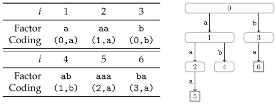
Figure 7. The LZ78 factorization and its LZ trie for the text $T=\mathtt{aaababaaaba}$. The xth factor is the concatenation of the edge labels of the path from the root to the node labeled with x. Its referred index is the label of its parent.

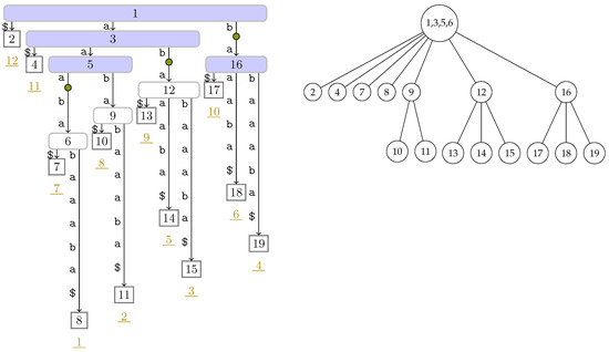
Figure 8. (Left) The suffix tree of T superimposed by the LZ trie (cf. Figure 7) computed on $T=\mathtt{aaababaaaba}\$$. Blue () colored $\mathsf{ST}$ nodes represent the explicit LZ trie nodes, i.e., those nodes that are present in $\mathsf{ST}$. Implicit LZ trie nodes are represented by the small rounded nodes (). The edge witnesses are the nodes with the preorder numbers 3, 5, 6, 12, and 16. (Right) $\mathsf{cpST}$ of T described in Section 4.8. The label of a node is the list of preorder numbers of the nodes in its respective heavy path. For instance, the heavy path from the root contains the nodes with the preorder numbers 1, 3, 5, and 6.

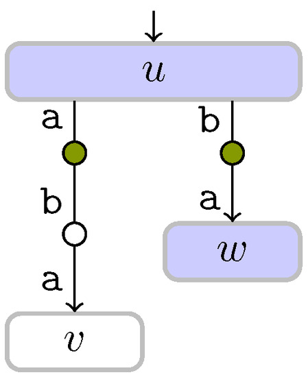
Figure 9. Excerpt of the suffix tree depicting three edge witnesses. Implicit trie node are represented by small rounded nodes (○), which are shaded if they are LZ trie nodes (). The explicit LZ trie nodes u and w are shaded in blue (). According to the figure, $n_v=1$ and $n_w=2$. In particular, the exploration counters of u and w are full.

However, since we do not know the shape of the LZ trie in advance, we also do not know which nodes will become an edge witness. For the time being, we augment each node with an exploration counter, spending $\mathcal{O}(nlgn)$ bits in total. As in Section 3, we assume that our text T has length n and ends with a special symbol $ smaller than all other characters appearing in T.

4.3. Linear-Time Computation

Now, we can give our first result of Theorem 2 on the LZ78 substring compression query problem by a simple modification of the LZ78 factorization algorithm presented by Nakashima et al. [45]. This algorithm uses a pointer-based suffix tree, which is augmented by a nearest marked ancestor data structure [47], using altogether $\mathcal{O}(nlgn)$ bits of space.

The algorithm works as follows: Suppose that we have computed the factors $F_1\cdots F_{x-1}$ and now want to compute $F_x$. Since $F_x$ is a prefix of the suffix $T[p..]$ with $p=|F_1\cdots F_{x-1}|+1$, $F_x$ is a prefix of the concatenation of edge labels on the path $\pi$ from the root to the leaf with suffix number p in the suffix tree. The additional requirement that $F_x$, excluding its last character, has to coincide with a preceding factor $F_y$ means that $F_y=F_x\left[1..\right|F_x|-1]$ is the string label of the lowest LZ trie node on $\pi$; this LZ trie node is represented either

• explicitly as an $\mathsf{ST}$ node w being the lowest edge witness on $\pi$; or
• implicitly by the exploration counter of w.

In either case, w is the edge witness of $F_y$ and determines its length $|F_y|=\mathrm{str}\_\mathrm{depth}\left(\mathrm{parent}\left(w\right)\right)+n_w$. We create an LZ trie node representing $F_x$ as follows:

• If $n_w$ is not full, we make w the edge witness of $F_x$, and increment $n_w$ by one.
• Otherwise ($n_w$ is full), we make the child $w^{\prime }$ of w on the path $\pi$ the edge witness of $F_x$, and set $n_{w^{\prime }}\leftarrow 1$.

It is left to find w, which we can by traversing $\pi$ from the root until reaching an edge $e=(u,v)$ whose exploration counter $n_v$ is less than the length of its label $c\left(e\right)$, where either u or v is w. However, a linear scan of $\pi$ for finding w would result in $\mathcal{O}\left(z\right)$ time per factor. Here, the fringe marked ancestor queries come into the picture, which allow us to find a lowest edge witness in amortized constant time: by marking all edge witnesses, querying the lowest marked ancestor of the leaf with suffix number p yields either u or v. This gives us $\mathcal{O}\left(1\right)$ amortized time per LZ78 factor, and concludes the LZ78 factorization algorithm of Nakashima et al. [45] (Theorem 3).

Finally, to obtain the LZ78 factorization of $T\left[\mathsf{b}\right(\mathcal{I}\left)..\mathsf{e}\right(\mathcal{I}\left)\right]$ for a given interval $\mathcal{I}$ with $\mathcal{I}=\left[\mathsf{b}\right(\mathcal{I}\left)..\mathsf{e}\right(\mathcal{I}\left)\right]$, we do not start the computation at $T[1..]$, but directly at $T\left[\mathsf{b}\right(\mathcal{I})..]$, and terminate when a factor ends at $T\left[\mathsf{e}\right(\mathcal{I}\left)\right]$ or protrudes $T\left[\mathcal{I}\right]$ to the right. In the latter case, we trim this factor. Hence, we can compute the factorization of $T\left[\mathcal{I}\right]$ in $\mathcal{O}\left(z_{78\left[\mathcal{I}\right]}\right)$ time with $\mathcal{O}(nlgn)$ bits of space, in which we can store a pointer-based suffix tree on T.

4.4. Outline

In what follows, we want to study variants of this algorithm that use more lightweight data structures at the expense of additional running times. All LZ78 factorization algorithms here presented stick to the following general framework, which we call a pass: For each leaf $\lambda$ whose suffix number is the starting position of a factor F, locate the lowest edge witness w on the path from the root to $\lambda$ and create a new LZ trie node by incrementing either $n_w$ or the exploration counter of its child on the path towards $\lambda$ as described in Section 4.3. Since w determines the length of the factor F, we know the suffix number of the leaf that starts with the next factor.

After a pass, we know the LZ trie topology due to the exploration counters. In a subsequent pass (Section 4.7), we use this knowledge to associate an edge witness w with the index of the most recent factor having w as its edge witness such that we can identify the referred indices with this association. However, before that, we reduce the space (Section 4.5) and subsequently show how to perform a pass within the reduced working space (Section 4.6). Finally, we accelerate a root-to-leaf traversal for long factors in Section 4.8.

4.5. Space-Efficient Computation

In what follows, we give trade-offs for less space but slightly larger time bounds by using SST and CST. To get below $\mathcal{O}(nlgn)$ bits of space, we need to get rid of: (a) the $\mathcal{O}(nlgn)$-bits marked ancestor data structure; and (b) the $\mathcal{O}(nlgn)$ bits for the exploration counters. For the latter (b), Fischer et al. [4] (Section 4.1) presented a data structure representing the exploration counters within $\mathcal{O}\left(n\right)$ bits on top of the suffix tree. For the former (a), we use level ancestor queries to simulate a fringe marked ancestor query: to this end, we mark all edge witnesses in a bit vector $B_E$ of length $2n$ such that $B_E\left[j\right]=1$ if and only if the $\mathsf{ST}$ node with preorder rank j is an edge witness (remember that the number of nodes in $\mathsf{ST}$ is at most $2n$). Suppose now that we want to compute the factor $F_x$. For that, we visit the leaf $\lambda$ with suffix number $\mathsf{b}\left(\mathcal{I}\right)+|F_1\cdots F_{x-1}|$. As in Section 4.3, we want to find the lowest edge witness on the path from the root to $\lambda$, which we find with a fringe marked ancestor query. Here, we answer this query by scanning the path from the root to $\lambda$ until reaching the lowest marked node in $B_E$. We can traverse linearly from the root to this node by querying $d\mapsto \mathrm{level}\_\mathrm{anc}(\lambda ,d)$ for each depth $d\ge 0$. However, we then visit $\mathcal{O}\left(\right|F_x\left|\right)$ nodes for computing the factor $F_x$, or $\mathcal{O}\left(\right|\mathcal{I}\left|\right)$ nodes in total. To improve this bound, we can apply again exponential search (cf. Figure 6). To see why that can be done, let $(v_0,\dots ,v_m)$ be the path from the root $v_0$ to $\lambda =v_m$. If each node $v_d$ (for each depth $d\in \left[0..m\right]$) is represented by its preorder number, then $B_E\left[v_0\right]\cdots B_E\left[v_m\right]=1^{k+1}{0}^{m-k}$ if the lowest edge witness has depth k, which is the smallest $k\le |F_x|$ such that $\mathrm{str}\_\mathrm{depth}(\mathrm{level}\_\mathrm{anc}(\lambda ,k))\ge |F_x|-1$. Although we do not know k in advance, we can find the rightmost ‘$1$’ in $B_E\left[v_0\right]\cdots B_E\left[v_m\right]$ with an exponential search visiting $\mathcal{O}(lgk)=\mathcal{O}(lg|F_x\left|\right)$ nodes (we evaluate $d\mapsto \mathrm{level}\_\mathrm{anc}(\lambda ,d)$ for specific d and check each time whether the returned node is marked in $B_E$). Thus, we can determine $|F_x|$ and $F_x$’s edge witness in $\mathcal{O}(lg|F_x\left|\right)$ time. Since $|F_x|\le x$, we spend $\mathcal{O}(z_{78\left[\mathcal{I}\right]}lg{z}_{78\left[\mathcal{I}\right]})$ time in total.

4.6. Navigation in Small Space

To complete our algorithm for SST and CST, it is left to study how to access the leaves when issuing the level ancestor queries. While the LZ78 factorization algorithms of Fischer et al. [4] used the fact that they can scan the leaves linearly in suffix number order to simulate the scan of the text in text order within their $\mathcal{O}\left(n\right)$ time budget, we want to accelerate this algorithm by visiting only the leaves whose suffix numbers match the starting positions of the factors. With the SST, we can select the leaf $\lambda$ with suffix number $i\in \left[1..n\right]$ in $\mathcal{O}(1/ϵ)$ time since we have access to $\mathsf{ISA}\left[i\right]$ returning the leaf-rank of $\lambda$.

With the CST, we can visit the leaf with the subsequent suffix number with $\mathrm{next}\_\mathrm{leaf}$ in constant time, but may need $\mathcal{O}\left(n\right)$ time to visit an arbitrary leaf. Here, the idea is to store a sampling of $\mathsf{ISA}$ within $\mathcal{O}(nlg\sigma )$ bits of space during a precomputation step. We can produce the values of this sampling by iterating over $\mathrm{next}\_\mathrm{leaf}$ such that we obtain an array that stores in its ith entry the leaf-rank of the leaf with suffix number $i{log}_{\sigma }n$. Consequently, we can jump to a leaf with suffix number $j\in \left[1..n\right]$ in $\mathcal{O}\left({log}_{\sigma }n\right)$ time by jumping to the closest sampled predecessor of j, and subsequently applying $\mathrm{next}\_\mathrm{leaf}$$\mathcal{O}\left({log}_{\sigma }n\right)$ times to reach the leaf with suffix number j. To sum up, we need $\mathcal{O}\left({log}_{\sigma }n\right)$ time to traverse between two corresponding leaves. The total time becomes $\mathcal{O}({ϵ}^{-1}{z}_{78\left[\mathcal{I}\right]}lg{z}_{78\left[\mathcal{I}\right]})$ and $\mathcal{O}\left(z_{78\left[\mathcal{I}\right]}(lg{z}_{78\left[\mathcal{I}\right]}+{log}_{\sigma }n)\right)$ for the SST and the CST, respectively.

4.7. LZ78 Coding

Finally, to obtain the LZ78 coding, we need to compute the referred indices. In a classic LZ78 trie, we would augment each trie node with the index of its corresponding factor. Here, we additionally need a trick for the implicitly represented LZ trie nodes: For them, we can now leverage the edge witnesses by augmenting each of them with the factor index of the currently lowest LZ trie node created on its ingoing edge. Fortunately, we know all nodes that become edge witnesses thanks to $B_E$ (cf. Section 4.5) marking the preorder numbers of all edge witnesses. We now enhance $B_E$ with a rank-support such that we can give each edge witness a rank within $\left[1..z_{78\left[\mathcal{I}\right]}\right]$. Therefore, we can maintain the most recent factor indices corresponding to each edge witness in an array W of $z_{78\left[\mathcal{I}\right]}lg{z}_{78\left[\mathcal{I}\right]}$ bits. We again conduct a pass as described in Section 4.4, but this time we use W to write out the referred indices (see ([4] [Section 4.2.1 Pass (b)]) for a detailed description on how to read the referred indices from W). By doing so, we finally obtain Theorem 2. For an overview, we present the obtained complexity bounds in Table 1.

Table 1. Complexities for answering an LZ78 substring compression query with different suffix tree representations. The query is on an interval $\mathcal{I}\subset \left[1..n\right]$. A query additionally needs an array of $z_{78\left[\mathcal{I}\right]}lgn=\mathcal{O}(nlg\sigma )$ bits of space as described in Section 4.7. If there are characters of the alphabet appearing nowhere in the text, we additionally need to keep the text available during a query, which adds $nlg\sigma$ bits to the query space complexity of the SST solution.

Construction
Data Structure	Time	Space in Bits
suffix tree [45]	$\mathcal{O}\left(n\right)$	$\mathcal{O}(nlgn)$
SST [4] [Section 2.2.3]	$\mathcal{O}\left(n{ϵ}^{-1}\right)$	$nlg\sigma +(1+ϵ)nlgn+\mathcal{O}\left(n\right)$
CST [4] [Section 2.2.2]	$\mathcal{O}\left(n\right)$	$\mathcal{O}(nlg\sigma )$
Query
Data Structure	Time	Space in Bits
suffix tree [45]	$\mathcal{O}\left(z_{78\left[\mathcal{I}\right]}\right)$	$\mathcal{O}(nlgn)$
SST [4] [Section 2.2.3]	$\mathcal{O}(z_{78\left[\mathcal{I}\right]}lg{z}_{78\left[\mathcal{I}\right]}{ϵ}^{-1})$	$((1+ϵ)n+z_{78\left[\mathcal{I}\right]})lgn+\mathcal{O}\left(n\right)$
CST [4] [Section 2.2.2]	$\mathcal{O}\left(z_{78\left[\mathcal{I}\right]}(lg{z}_{78\left[\mathcal{I}\right]}+{log}_{\sigma }n)\right)$	$\mathcal{O}(nlg\sigma )$

4.8. Centroid-Path Decomposed Suffix Tree

If the length $\ell \le z_{78\left[\mathcal{I}\right]}$ of the longest factor is so large that $lg\ell =\omega (lglgn)$, then we can speed up the exponential search of Section 4.5 by searching in the centroid-path decomposed suffix tree $\mathsf{cpST}$. The centroid path decomposition [49] of the suffix tree is defined as follows: For each internal node, we call its child whose subtree is the largest among all its siblings (ties are broken arbitrarily if there are multiple such children) a heavy node, while we call all other children light nodes. Additionally, we make the root and all leaves light nodes (here we differ from the standard definition because we need a one-to-one relationship between leaves in the original tree and in the path-decomposed one). A heavy path is a path from a light node u to the parent of a leaf containing, except for u, only heavy nodes. There is a one-to-one relationship between light nodes and heavy paths. Since heavy paths do not overlap, we can contract all heavy paths to single nodes and thus form $\mathsf{cpST}$ (see ([49] [Section 4.2]) for details and Figure 8 for an example). The centroid path decomposition is helpful, because the number of light nodes on a path from the root to a leaf is $\mathcal{O}(lgn)$, which means that a path from the root to a leaf in $\mathsf{cpST}$ contains $\mathcal{O}(lgn)$ nodes. This can be seen by the fact that the subtree size of a light node is at most half of the subtree size of its heavy sibling; thus, when visiting a light node during a top-down traversal in $\mathsf{ST}$, we at least half the number of $\mathsf{ST}$ nodes we can visit from then on. Consequently, a root-to-leaf path in $\mathsf{cpST}$ has $\mathcal{O}(lgn)$ nodes.

For that to be of use, we need a connection between $\mathsf{ST}$ and $\mathsf{cpST}$: observe that the number of leaves and their respective order is the same in both trees, such that we can map leaves by their leaf-ranks in constant time. If we mark the light nodes in the suffix tree in a bit vector $B_L$, then the rank of a light node v in $B_L$ is the preorder number of the node in $\mathsf{cpST}$ representing the heavy path whose highest node is v. To stay within our space budget, we represent the tree topology of $\mathsf{cpST}$ with a BP sequence (which we briefly introduced in Section 2). First, we mark all light nodes in $B_L$ by an Euler tour, where we query the $\mathsf{ST}$ topology for the subtree size rooted at an arbitrary node in constant time. Next, we perform a depth-first search traversal on the suffix tree while producing the BP sequence of $\mathsf{cpST}$. For that, we use a stack to store the light node ancestors of the currently visited node. Since a node has $\mathcal{O}(lgn)$ light nodes as ancestors, the stack uses $\mathcal{O}\left({lg}^{2}n\right)$ bits of space. Finally, we endow $B_L$ with a select-support such that we can map a node of $\mathsf{cpST}$ to its corresponding light node in $\mathsf{ST}$.

Our algorithm conducting a pass works as follows: Suppose that we visit the leaf $\lambda$ with suffix number $\mathsf{b}\left(\mathcal{I}\right)+|F_1|+\cdots +|F_{x-1}|$. This time, we map $\lambda$ to the leaf ${\lambda }^{\prime }$ of $\mathsf{cpST}$ having the same leaf-rank as $\lambda$ in $\mathsf{ST}$. Next, we apply the exponential search with $d\mapsto \mathrm{level}\_\mathrm{anc}({\lambda }^{\prime },d)$ on $\mathsf{cpST}$, to obtain a $\mathsf{cpST}$ node representing the heavy path whose highest node is a light node v, i.e., v is the lowest light node on the $\mathsf{ST}$ path from the root to the leaf $\lambda$ that is an edge witness. Since a root-to-leaf path in $\mathsf{ST}$ has $\mathcal{O}(lgn)$ light nodes, we spend $\mathcal{O}(min(lg|F_x|,lglgn))$ time to find v.

Finally, it is left to move from v to the lowest edge witness on the path from v to $\lambda$ in $\mathsf{ST}$. For that, we use a dictionary $\mathcal{D}$ that associates a light node with the number of edge witnesses in its heavy path. This number is at most $z_{78\left[\mathcal{I}\right]}\le \left|\mathcal{I}\right|$, and thus it can be stored in $lg\left|\mathcal{I}\right|$ bits, while a light node can be represented with its preorder number in $\mathcal{O}(lgn)$ bits. $\mathcal{D}$ has to be dynamic since we do not know in advance which nodes will become edge witnesses; we can make use of one of the dynamic dictionaries given in Table 2, where $t_{\mathcal{D}}$ denotes the time for an operation such as a lookup or an insertion and $s_{\mathcal{D}}$ denotes the dictionary size in bits.

Table 2. Dynamic dictionary representations usable in our $\mathsf{cpST}$ approach (cf. Section 4.8) for $\mathcal{D}$ mapping a light node represented in $lgn$ bits to the lowest edge witness within its heavy path represented in $lg\left|\mathcal{I}\right|$ bits. $z:=z_{78\left[\mathcal{I}\right]}$ denotes the number of LZ78 factors of $T\left[\mathcal{I}\right]$, which is an upper bound on the number of edge witnesses. An operation is a lookup or an insertion. We are interested in instances with $t_{\mathcal{D}}=o(lgz)$ (since, otherwise, the approach of Section 4.5 is favorable). $ϵ\in (0,1)$ is a selectable constant.

Data Structure $\mathcal{D}$	Operation Time ${\mathit{t}}_{\mathcal{D}}$	Space ${\mathit{s}}_{\mathcal{D}}$ in Bits
plain array	$\mathcal{O}\left(1\right)$	$nlg\left|\mathcal{I}\right|$
Raman et al. [50]	$\mathcal{O}(lgz/lglgz)$ amortized	$zlg\left(n\right|\mathcal{I}\left|\right)+o\left(z\right)$
backyard Cuckoo hashing [51]	$\mathcal{O}(lg(1/ϵ)/{ϵ}^2)$ expected	$(1+ϵ)zlg\left(n\right|\mathcal{I}\left|\right)$

Now, suppose that $\mathcal{D}$ stores that d nodes in v’s heavy path are edge witnesses. Let w be the next light node on the path from v to $\lambda$ (i.e., w is the highest light node on the path from the root to $\lambda$ whose exploration counter is still zero).

• If $d-1$ is at least the height difference between v and w, then the parent u of w is already an edge witness, and u is a node on the heavy path of v. If the exploration counter of u is full, i.e., $n_u=c(\mathrm{parent}\left(u\right),u)$, then we increment the exploration counter of w, and hence make w an edge witness and add w to $\mathcal{D}$.
• Otherwise ($d-1$ is smaller than this height difference), the node whose exploration counter we want to increment is within the heavy path, and is either the dth or $(d+1)$th descendent of v.

In total, for $z:=z_{78\left[\mathcal{I}\right]}$, we can improve the $zlgz$ factor in the time bounds to $z·min(lgz,t_{\mathcal{D}}+lglgn)$, which is $z·min(lgz,lgz/lglgz+lglgn)$ when implementing $\mathcal{D}$ with the dynamic dictionary of Raman et al. [50], costing $s_{\mathcal{D}}=zlg\left(nz\right)+o\left(z\right)$ bits of additional working space during a query. More formally:

Theorem 4.

Given a text $T\left[1..n\right]$ of length n whose characters are drawn from an alphabet with size $\sigma =n^{\mathcal{O}\left(1\right)}$, we can compute a data structure on T in $\mathcal{O}\left(n\right)$ time that computes, given an interval $\mathcal{I}\subset \left[1..n\right]$, the LZ78 factorization of $T\left[\mathcal{I}\right]$ in

• $\mathcal{O}\left(z_{78\left[\mathcal{I}\right]}({log}_{\sigma }n+min(lg{z}_{78\left[\mathcal{I}\right]},t_{\mathcal{D}}+lglgn))\right)$ time using $\mathcal{O}(nlg\sigma )+s_{\mathcal{D}}$ bits of space, or
• $\mathcal{O}({ϵ}^{-1}{z}_{78\left[\mathcal{I}\right]}min(lg{z}_{78\left[\mathcal{I}\right]},t_{\mathcal{D}}+lglgn))$ time using $(1+ϵ)nlgn+s_{\mathcal{D}}+\mathcal{O}\left(n\right)$ bits of space,

where $z_{78\left[\mathcal{I}\right]}$ is the number of computed LZ78 factors, $ϵ\in (0,1]$ is a selectable constant, and $t_{\mathcal{D}}$ and $s_{\mathcal{D}}$ are the time and space complexities of a dynamic dictionary associating a $lgn$-bit integer with a $lg\left|\mathcal{I}\right|$-bit value (cf. Table 2). Similar to Theorem 2, we need the read-only text stored for queries if there is a character in the alphabet that does not appear in T.

5. Conclusions

We used techniques introduced by Fischer et al. [4], which work on the succinct suffix tree (SST) and the compressed suffix tree (CST), to tackle the non-overlapping LZSS factorization and the LZ78 substring compression query problem. One of the main techniques is the usage of level ancestor queries to traverse a root-to-leaf path. For computing the non-overlapping LZSS factorization, our idea was to merge these techniques with the algorithm of Gusfield [31] working in root-to-leaf traversals. To answer an LZ78 substring compression query, we combined exponential search with the level ancestor queries and could accelerate this by first searching in the centroid path-decomposed suffix tree $\mathsf{cpST}$ whenever the factor lengths become large.

We wonder whether we can improve the space bounds for solving the semi-dynamic fringe marked ancestor problem (addressed in Section 4), where updates are restricted to marking a node that is a child of an already marked node; hence, the marked nodes form a connected subgraph of the suffix tree sharing at least the root. Without the need of the $\mathcal{O}\left(n\right)$ words for the marked ancestor data structure, it becomes interesting to devise algorithms computing the reversed LZSS factorization [52] (see ([53] [Chapter 3.6.2])) in low memory.

References

- Ziv, J.; Lempel, A. A universal algorithm for sequential data compression. IEEE Trans. Inf. Theory 1977, 23, 337–343. [Google Scholar] [CrossRef]
- Ziv, J.; Lempel, A. Compression of individual sequences via variable-rate coding. IEEE Trans. Inf. Theory 1978, 24, 530–536. [Google Scholar] [CrossRef]
- Storer, J.A.; Szymanski, T.G. Data compression via textural substitution. J. ACM 1982, 29, 928–951. [Google Scholar] [CrossRef]
- Fischer, J.; Tomohiro, I.; Köppl, D.; Sadakane, K. Lempel-Ziv Factorization Powered by Space Efficient Suffix Trees. Algorithmica 2018, 80, 2048–2081. [Google Scholar] [CrossRef]
- Crochemore, M.; Tischler, G. Computing Longest Previous non-overlapping Factors. Inf. Process. Lett. 2011, 111, 291–295. [Google Scholar] [CrossRef]
- Cormode, G.; Muthukrishnan, S. Substring compression problems. In Proceedings of the SODA, Vancouver, BC, Canada, 23–25 January 2005; pp. 321–330. [Google Scholar]
- Jacobson, G. Space-efficient Static Trees and Graphs. In Proceedings of the FOCS, Research Triangle Park, NC, USA, 30 October–1 November 1989; pp. 549–554. [Google Scholar]
- Clark, D.R. Compact Pat Trees. Ph.D. Thesis, University of Waterloo, Waterloo, ON, Canada, 1996. [Google Scholar]
- Manber, U.; Myers, E.W. Suffix Arrays: A New Method for On-Line String Searches. SIAM J. Comput. 1993, 22, 935–948. [Google Scholar] [CrossRef]
- Sadakane, K. Compressed Suffix Trees with Full Functionality. Theory Comput. Syst. 2007, 41, 589–607. [Google Scholar] [CrossRef]
- Grossi, R.; Vitter, J.S. Compressed Suffix Arrays and Suffix Trees with Applications to Text Indexing and String Matching. SIAM J. Comput. 2005, 35, 378–407. [Google Scholar] [CrossRef]
- Hon, W.; Sadakane, K.; Sung, W. Breaking a Time-and-Space Barrier in Constructing Full-Text Indices. SIAM J. Comput. 2009, 38, 2162–2178. [Google Scholar] [CrossRef]
- Munro, J.I.; Navarro, G.; Nekrich, Y. Space-Efficient Construction of Compressed Indexes in Deterministic Linear Time. In Proceedings of the SODA, Barcelona, Spain, 16–19 January 2017; pp. 408–424. [Google Scholar]
- Navarro, G.; Sadakane, K. Fully Functional Static and Dynamic Succinct Trees. ACM Trans. Algorithms 2014, 10, 16:1–16:39. [Google Scholar] [CrossRef]
- Kosolobov, D.; Shur, A.M. Comparison of LZ77-type parsings. Inf. Process. Lett. 2019, 141, 25–29. [Google Scholar] [CrossRef]
- Kolpakov, R.M.; Kucherov, G. Finding approximate repetitions under Hamming distance. Theor. Comput. Sci. 2003, 303, 135–156. [Google Scholar] [CrossRef]
- Duval, J.; Kolpakov, R.; Kucherov, G.; Lecroq, T.; Lefebvre, A. Linear-time computation of local periods. Theor. Comput. Sci. 2004, 326, 229–240. [Google Scholar] [CrossRef][Green Version]
- Kociumaka, T.; Kubica, M.; Radoszewski, J.; Rytter, W.; Walen, T. A linear time algorithm for seeds computation. In Proceedings of the SODA, Kyoto, Japan, 17–19 January 2012; pp. 1095–1112. [Google Scholar]
- Butrak, T.; Chairungsee, S. A Linear Time Algorithm for Finding Tandem Repeat in DNA Sequences. In Proceedings of the ICIT, Melbourne, Australia, 13–15 February 2019; pp. 426–429. [Google Scholar]
- Lothaire, M. Applied Combinatorics on Words; Encyclopedia of Mathematics and Its Applications, Cambridge University Press: Cambridge, UK, 2005. [Google Scholar]
- Crochemore, M.; Iliopoulos, C.S.; Kubica, M.; Rytter, W.; Walen, T. Efficient algorithms for three variants of the LPF table. J. Discret. Algorithms 2012, 11, 51–61. [Google Scholar] [CrossRef]
- Chairungsee, S.; Butrak, T.; Chareonrak, S.; Charuphanthuset, T. Longest Previous Non-overlapping Factors Computation. In Proceedings of the DEXA, Valencia, Spain, 1–4 September 2015; pp. 5–8. [Google Scholar]
- Chairungsee, S.; Crochemore, M. Longest Previous Non-overlapping Factors Table Computation. In Proceedings of the COCOA, LNCS, Shanghai, China, 16–18 December 2017; Volume 10628, pp. 483–491. [Google Scholar]
- Chairungsee, S. Efficient Approaches to Compute Longest Previous Non-overlapping Factor Array. Fundam. Inform. 2018, 163, 291–304. [Google Scholar] [CrossRef]
- Ohlebusch, E.; Weber, P. On the Computation of Longest Previous Non-overlapping Factors. In Proceedings of the SPIRE, LNCS, Segovia, Spain, 7–9 October 2019; Volume 11811, pp. 372–381. [Google Scholar]
- Crochemore, M.; Ilie, L. Computing Longest Previous Factor in linear time and applications. Inf. Process. Lett. 2008, 106, 75–80. [Google Scholar] [CrossRef]
- Bannai, H.; Inenaga, S.; Köppl, D. Computing All Distinct Squares in Linear Time for Integer Alphabets. In Proceedings of the CPM, LIPIcs, Copenhagen, Denmark, 17–19 June 2017; Volume 78, pp. 22:1–22:18. [Google Scholar]
- Ferragina, P.; Manzini, G. Opportunistic Data Structures with Applications. In Proceedings of the FOCS, Redondo Beach, CA, USA, 12–14 November 2000; pp. 390–398. [Google Scholar]
- Okanohara, D.; Sadakane, K. An Online Algorithm for Finding the Longest Previous Factors. In Proceedings of the ESA, LNCS, Karlsruhe, Germany, 15–17 September 2008; Volume 5193, pp. 696–707. [Google Scholar]
- Prezza, N.; Rosone, G. Faster Online Computation of the Succinct Longest Previous Factor Array. In Proceedings of the CiE, LNCS, Fisciano, Italy, 29 June–3 July 2020; Volume 12098, pp. 339–352. [Google Scholar]
- Gusfield, D. Algorithms on Strings, Trees, and Sequences: Computer Science and Computational Biology; Cambridge University Press: Cambridge, UK, 1997. [Google Scholar]
- Fischer, J.; Heun, V. Space-Efficient Preprocessing Schemes for Range Minimum Queries on Static Arrays. SIAM J. Comput. 2011, 40, 465–492. [Google Scholar] [CrossRef]
- Fischer, J.; Mäkinen, V.; Navarro, G. Faster entropy-bounded compressed suffix trees. Theor. Comput. Sci. 2009, 410, 5354–5364. [Google Scholar] [CrossRef]
- Keller, O.; Kopelowitz, T.; Feibish, S.L.; Lewenstein, M. Generalized substring compression. Theor. Comput. Sci. 2014, 525, 42–54. [Google Scholar] [CrossRef]
- Matsuda, K.; Sadakane, K.; Starikovskaya, T.; Tateshita, M. Compressed Orthogonal Search on Suffix Arrays with Applications to Range LCP. In Proceedings of the CPM, LIPIcs, Aarhus, Denmark, 30 June–2 July 2020; Volume 161, pp. 23:1–23:13. [Google Scholar]
- Bille, P.; Gørtz, I.L.; Steiner, T.A. String Indexing with Compressed Patterns. In Proceedings of the STACS, LIPIcs, Montpelier, France, 10–13 March 2020; Volume 154, pp. 10:1–10:13. [Google Scholar]
- Bentley, J.L.; Yao, A.C. An Almost Optimal Algorithm for Unbounded Searching. Inf. Process. Lett. 1976, 5, 82–87. [Google Scholar] [CrossRef]
- Lifshits, Y. Solving Classical String Problems an Compressed Texts. In Proceedings of the Combinatorial and Algorithmic Foundations of Pattern and Association Discovery, Dagstuhl Seminar Proceedings, Dagstuhl, Germany, 14–19 March 2006. Number 06201. [Google Scholar]
- Fischer, J.I.T.; Köppl, D. Deterministic Sparse Suffix Sorting in the Restore Model. ACM Trans. Algorithms 2020, 16, 50:1–50:53. [Google Scholar] [CrossRef]
- Maruyama, S.; Nakahara, M.; Kishiue, N.; Sakamoto, H. ESP-index: A compressed index based on edit-sensitive parsing. J. Discret. Algorithms 2013, 18, 100–112. [Google Scholar] [CrossRef]
- Cormode, G.; Muthukrishnan, S. The string edit distance matching problem with moves. ACM Trans. Algorithms 2007, 3, 2:1–2:19. [Google Scholar] [CrossRef]
- Charikar, M.; Lehman, E.; Liu, D.; Panigrahy, R.; Prabhakaran, M.; Sahai, A.; Shelat, A. The smallest grammar problem. IEEE Trans. Inf. Theory 2005, 51, 2554–2576. [Google Scholar] [CrossRef]
- Bannai, H.; Gawrychowski, P.; Inenaga, S.; Takeda, M. Converting SLP to LZ78 in almost Linear Time. In Proceedings of the CPM, LNCS, Bad Herrenalb, Germany, 17–19 June 2013; Volume 7922, pp. 38–49. [Google Scholar]
- Rytter, W. Application of Lempel-Ziv factorization to the approximation of grammar-based compression. Theor. Comput. Sci. 2003, 302, 211–222. [Google Scholar] [CrossRef]
- Nakashima, Y.; Tomohiro, I.; Inenaga, S.; Bannai, H.; Takeda, M. Constructing LZ78 tries and position heaps in linear time for large alphabets. Inf. Process. Lett. 2015, 115, 655–659. [Google Scholar] [CrossRef]
- Jansson, J.; Sadakane, K.; Sung, W. Linked Dynamic Tries with Applications to LZ-Compression in Sublinear Time and Space. Algorithmica 2015, 71, 969–988. [Google Scholar] [CrossRef]
- Alstrup, S.; Husfeldt, T.; Rauhe, T. Marked Ancestor Problems. In Proceedings of the FOCS, Palo Alto, CA, USA, 8–11 November 1998; pp. 534–544. [Google Scholar]
- Breslauer, D.; Italiano, G.F. Near real-time suffix tree construction via the fringe marked ancestor problem. J. Discret. Algorithms 2013, 18, 32–48. [Google Scholar] [CrossRef]
- Ferragina, P.; Grossi, R.; Gupta, A.; Shah, R.; Vitter, J.S. On searching compressed string collections cache-obliviously. In Proceedings of the PODS, Vancouver, BC, Canada, 9–11 June 2008; pp. 181–190. [Google Scholar]
- Raman, R.; Raman, V.; Rao, S.S. Succinct Dynamic Data Structures. In Proceedings of the WADS, LNCS, Providence, RI, USA, 8–10 August 2001; Volume 2125, pp. 426–437. [Google Scholar]
- Arbitman, Y.; Naor, M.; Segev, G. Backyard Cuckoo Hashing: Constant Worst-Case Operations with a Succinct Representation. In Proceedings of the FOCS, Las Vegas, NV, USA, 23–26 October 2010; pp. 787–796. [Google Scholar]
- Kolpakov, R.; Kucherov, G. Searching for gapped palindromes. Theor. Comput. Sci. 2009, 410, 5365–5373. [Google Scholar] [CrossRef][Green Version]
- Köppl, D. Exploring Regular Structures in Strings. Ph.D. Thesis, TU Dortmund, Dortmund, Germany, 2018. [Google Scholar]
Publisher’s Note: MDPI stays neutral with regard to jurisdictional claims in published maps and institutional affiliations. |
© 2021 by the author. Licensee MDPI, Basel, Switzerland. This article is an open access article distributed under the terms and conditions of the Creative Commons Attribution (CC BY) license (http://creativecommons.org/licenses/by/4.0/).