Goal Oriented Time Adaptivity Using Local Error Estimates

Abstract

We consider initial value problems (IVPs) where we are interested in a quantity of interest (QoI) that is the integral in time of a functional of the solution. For these, we analyze goal oriented time adaptive methods that use only local error estimates. A local error estimate and timestep controller for step-wise contributions to the QoI are derived. We prove convergence of the error in the QoI for tolerance to zero under a controllability assumption. By analyzing global error propagation with respect to the QoI, we can identify possible issues and make performance predictions. Numerical tests verify these results. We compare performance with classical local error based time-adaptivity and a posteriori based adaptivity using the dual-weighted residual (DWR) method. For dissipative problems, local error based methods show better performance than DWR and the goal oriented method shows good results in most examples, with significant speedups in some cases.

1. Introduction

A typical situation in numerical simulations based on differential equations is that one is not interested in the solution per se but in a Quantity of Interest (QoI) that is given as a functional of the solution. When designing an airplane, the QoI would be the lift coefficient divided by the drag coefficient. In simulations of the Greenland ice sheet, it could be the net amount of ice loss over a year [1]. For wind turbine design, the amount of energy produced during a certain time period is more important than the actual flow solution. Other examples are in optimization with ODEs or PDEs as constraints. In the turbine example, one may want to optimize blade shape [2] or determine optimal placement of, for example, tidal turbines [3], for maximal energy output.

In this article, we consider time-dependent problems with a QoI as follows:

$$\begin{array}{cc}\hfill \mathrm{IVP}:& \dot{\mathit{u}}\left(t\right)=\mathit{f}(t,\mathit{u}\left(t\right)),t\in [t_0,t_e],\mathit{u}\left(t_0\right)={\mathit{u}}_0,\mathit{f}:[t_0,t_e]\times {\mathbb{R}}^d\to {\mathbb{R}}^d\hfill \end{array}$$

(1)

$$\begin{array}{cc}\hfill \mathrm{QoI}:& \mathcal{J}\left(\mathit{u}\right):={\int }_{t_0}^{t_e}j(t,\mathit{u}\left(t\right))\mathtt{d}t,j:[t_0,t_e]\times {\mathbb{R}}^d\to \mathbb{R}\hfill \end{array}$$

(2)

The goal is to find an adaptive time discretization to reduce computational costs. An adaptive method consists of a time-integration scheme for Equation (1), an error estimator, a timestep controller and a discretization scheme for Equation (2). The input for an adaptive method is a tolerance $\tau$ and initial timestep $\Delta t_0$. The output is an approximation to the solution, this can be a discrete solution ${\mathit{u}}_h\approx \mathit{u}$, or ${\mathcal{J}}_h\left({\mathit{u}}_h\right)$.

Definition 1.

An adaptive method for Equation (1) is called convergent, if

$$\parallel \mathit{u}\left(t_e\right)-{\mathit{u}}_N\parallel \to 0\mathit{for}\tau \to 0,$$

where${\mathit{u}}_N\approx \mathit{u}\left(t_e\right)$. An adaptive method for Equations (1) and (2) is called convergent in the QoI, if

$$|\mathcal{J}\left(\mathit{u}\right)-{\mathcal{J}}_h\left({\mathit{u}}_h\right)|\to 0\mathit{for}\tau \to 0.$$

The standard approach for goal oriented adaptivity is the dual weighted residual (DWR) method [4,5]. It is most commonly used in the context of space-adaptivity for PDEs, but there is also work specifically on time-adaptivity [6,7,8]. DWR uses the adjoint (dual) problem to perform a posteriori adaptivity and get error bounds for the QoI.

In the time dependent case, the adjoint problem is a terminal value problem, i.e., an IVP backwards in time. The method yields global error estimates (bounds for linear problems). These error estimates are obtained by subsequently integrating forward and backward in time, storing both solutions. The estimates contain local information used to refine the discretization. This iterative process is repeated until a discretization is found with an error estimate $\eta \left({\mathit{u}}_h\right)$ that fulfills

$$|\mathcal{J}\left(\mathit{u}\right)-{\mathcal{J}}_h\left({\mathit{u}}_h\right)|\approx \eta \left({\mathit{u}}_h\right)\le \tau .$$

The resulting grids are typically of higher quality than those of local error based adaptive methods, particularly for advection dominated PDEs with spatially local QoIs.

The major drawback of this method is its cost, both in implementation and computation. To reduce computational effort, [9] suggested to apply the approach in a block-wise manner, thus making it more local. The method requires a variational formulation and is thus typically used in the context of Galerkin type schemes but can also be used, for example, for linear multistep methods [10].

Alternatives are classical adaptive methods for IVPs (Equation (1)) based on local error estimation. Convergence results are well established and described in standard textbooks [11,12]. They do not yield global error bounds. However, the error estimate is cheap and works very well for stiff problems, which typically have a dissipation mechanism to a base solution. We aim to extend these methods to problems like in Equations (1) and (2).

One way to include the QoI [13] is to reformulate Equations (1) and (2) as

$$\frac{d}{dt}\left[\begin{array}{c}\mathit{u}\left(t\right)\\ J\left(t\right)\end{array}\right]=\left[\begin{array}{c}\mathit{f}(t,\mathit{u}(t\left)\right)\\ j(t,\mathit{u}(t\left)\right)\end{array}\right],t\in [t_0,t_e],\left[\begin{array}{c}\mathit{u}\left(t_0\right)\\ J\left(t_0\right)\end{array}\right]=\left[\begin{array}{c}{\mathit{u}}_0\\ 0\end{array}\right].$$

(3)

We then have $J\left(t_e\right)={\int }_{t_0}^{t_e}j(t,\mathit{u}\left(t\right))dt=\mathcal{J}\left(\mathit{u}\right)$. Solving Equation (3) using an adaptive method based on the norm of the local error, the additional term coming from the added equation acts as a quadrature error estimate. In our numerical tests, this additional term is negligible in comparison to the local error in $\mathit{u}$, and thus there is no benefit compared to the classic method. Here, $\mathcal{J}$ is discretized using the quadrature scheme defined by time-integration. This choice has an impact on performance, but we do not have conclusive results when it is beneficial or detrimental.

A different approach is to combine the classic adaptive method with an error estimate that uses local errors in the QoI only [14]. This way, the hope is to be more efficient than either DWR or the classic approach by having a cheap error estimate, focusing on direct error contributions to the QoI. One only requires additional evaluations of $j(t,\mathit{u}(t\left)\right)$ to compute the error estimate. This makes it notably less intrusive to implement compared to DWR and suitable for partitioned approaches to coupled systems, since it only requires a local error estimate.

Methods in this spirit have been proposed before. John and Rang conceptualize this idea for drag and lift coefficients in incompressible flows [15]. Turek predicts “catastrophical results” [16] for a problem with an alternating lift coefficient due to vanishing error estimates. As a remedy, Turek proposes the usage of multiple QoIs for error estimation and does so using pressure, velocity, lift and drag. Wick et al. use a point-wise evaluation of the displacement field in fluid-structure interaction [17,18]. The authors get good results in two test cases, in one of which they observe slightly larger errors for too large tolerances. However, in all of the above cases, usage of this approach is heuristic and no analysis is presented.

Thus the question arises if these reports can be explained and could have been expected. The purpose of this article is to present a formal derivation and analysis of such a goal oriented adaptive method based on local error estimates, allowing us to answer this question in detail. To this end, we estimate the contribution per timestep to the error in the QoI. It consists of both quadrature and time-integration errors. We then derive local error estimates for these and use them in a deadbeat controller.

For the new adaptive method, we show convergence in the solution under a controllability condition with additional requirements on the timesteps. To obtain tolerance proportionality, i.e., $|\mathcal{J}\left(\mathit{u}\right)-{\mathcal{J}}_h\left({\mathit{u}}_h\right)|=\mathcal{O}\left(\tau \right)$ (we define $\mathit{e}\left(t\right)=\mathcal{O}\left(t^q\right)$, iff $\exists C>0,\delta >0:\parallel \mathit{e}\left(t\right)\parallel \le C{t}^q,\forall 0<t\le \delta$), for the error in the QoI when using higher order (>2) time-integration schemes, one needs solutions of sufficiently high order in intermediate points.

We do our analysis for embedded RK schemes [11] and a deadbeat timestep controller. The structure of our proof allows for simple convergence proofs of other controllers, for example, PID controllers [19], based on similarity to the deadbeat controller. To make statements on the performance of the goal oriented adaptive method, we analyze the impact of error dynamics on the error in the QoI.

We use numerical tests with widely different global error behaviors with respect to the QoI. For these, we confirm the convergence results and are able to explain the performance results. Our results show that the local error based methods are much more efficient than the DWR method for dissipative problems. It turns out to be relatively easy to predict bad performance, but harder to predict performance improvements. The goal oriented adaptive method shows good performance in most cases and significant speedups in some.

The structure of the article is as follows: We first review current adaptive methods in Section 2 and Section 3, then we explain and analyze our approach in Section 4. Numerical results are presented in Section 5.

2. A Posteriori Error Estimation Via the Dual Weighted Residual Method

The starting point of the DWR method for time dependent problems is an IVP in variational formulation: Find $u\in U$, resp. $u_h\in U_h$, such that

$$A(u;v)=F\left(v\right),\forall v\in V,\mathrm{resp}.A(u_h;v_h)=F\left(v_h\right),\forall v_h\in V_h.$$

(4)

Here, U and V are appropriate spaces, A is linear in v and possibly nonlinear in u. For the discrete problem in Equation (4), $U_h\subset U$ and $V_h\subset V$ are finite element spaces in time.

2.1. The Error Estimate

To estimate the error $e^{\mathcal{J}}=\mathcal{J}\left(u\right)-\mathcal{J}\left(u_h\right)$ in the QoI, see Equation (2), one uses the linearised adjoint problem for $\mathcal{J}\left(u\right)$: Find $z\in V$, resp. $z_h\in V_h$, such that

$$A^{\prime }(u;v,z)={\mathcal{J}}^{\prime }(u;v),\forall v\in U,\mathrm{resp}.A^{\prime }(u_h;v_h,z_h)={\mathcal{J}}^{\prime }(u_h;v_h),\forall v_h\in U_h,$$

(5)

where $A^{\prime }$ and ${\mathcal{J}}^{\prime }$ are the Gateaux derivatives of A and $\mathcal{J}$ with respect to u in direction v. The adjoint problem is a terminal value problem (IVP backwards in time) with $z\left(t_e\right)=0$.

An approximation of the error in the QoI is given by

$$e^{\mathcal{J}}\lesssim A(u_h,z-z_h)-F(z-z_h),$$

with equality for linear functionals and approximate upper bounds otherwise. Using an approximation $z_h^{+}\approx z$, which is of higher accuracy than $z_h$, using for example, higher order interpolation or a discrete solution on a finer grid [20], one gets a computable estimate

$$e^{\mathcal{J}}\lesssim \eta \left(u_h\right):=A(u_h,z_h^{+}-z_h)-F(z_h^{+}-z_h).$$

(6)

This can be further bounded by decomposing it by timesteps and thus giving a guide on where and how to adapt. For this to work, it is imperative that the solutions of the primal and adjoint problems are obtained at all points. This can cause storage problems for long time simulations and can be dealt with using check-pointing [21].

2.2. Adaptation Scheme

For a given initial grid, the DWR method is as follows

• Solve forward Problem (4) to obtain $u_h$.
• Construct and solve adjoint Problem (5) to obtain $z_h$.
• Calculate $z_h^{+}\approx z$ and the error estimate $\eta \left(u_h\right)$.
• Check $\eta \left(u_h\right)\le \tau$, if not met, refine grids and restart with new initial grid.

The scheme is very expensive due to the need of solving adjoint problems to obtain the error estimate. While one can use generic schemes to adapt grids, the adjoint problem and the error estimate are problem specific. Construction and solution of the adjoint problem can be automated using software such as dolfin-adjoint [22]. An advantage of the method is that the error estimate is global and one can expect the resulting discretizations to be of high quality.

We use a finer grid to approximate z by $z_h^{+}$, making this the most expensive step in the computation of $\eta \left(u_h\right)$. There are cheaper but less accurate ways to compute $z_h^{+}$, see [4]. These, however, increase the complexity of implementation even further.

3. Time Adaptivity Based on Local Error Estimates

The second adaptive method is the standard in ODE solvers. This method uses local error estimates and does not yield global error bounds or near optimal grids, but works very well in practice and is computationally cheap. It is convergent under a smoothness assumption.

The results from this section for one-step methods and the deadbeat controller (Equation (10)) are in principal classic [23]. Here, we present a new convergence proof, following the same principle techniques as in [23], but separating requirements on the error estimate, timesteps, and $\Delta t_0$, for generic one-step methods. This prepares convergence proofs for general controllers and estimates, and we use it to show convergence in the QoI for the goal oriented adaptive method in Section 4. We first introduce the relevant notation.

Definition 2.

The flow [24] of an IVP (Equation (1)) is the map

$${\mathcal{M}}^{t,\Delta t}:\mathit{u}\left(t\right)\to \mathit{u}(t+\Delta t),$$

where$t\in [t_0,t_e]$and$t+\Delta t\le t_e$for$\Delta t>0$.

The flow is the solution operator for $\mathit{u}\left(t\right)$. To numerically solve an IVP means to approximate the flow by a numerical flow map${\mathcal{N}}^{t,\Delta t}:{\mathbb{R}}^d\to {\mathbb{R}}^d$ defined by some numerical scheme. The solution after a timestep can be written in the form

$${\mathit{u}}_{n+1}={\mathcal{N}}^{t_n,\Delta t_n}{\mathit{u}}_n.$$

We generally assume Problem (1) to have the unique solution $\mathit{u}$ guaranteeing existence of the flow map ${\mathcal{M}}^{t,\Delta t}$. We define the global error by

$$\begin{array}{cc}\hfill {\mathit{e}}_{n+1}& :={\mathit{u}}_{n+1}-\mathit{u}\left(t_{n+1}\right)\hfill \\ & =\underset{\mathrm{global}\mathrm{error}\mathrm{increment}}{\underbrace{({\mathcal{N}}^{t_n,\Delta t_n}-{\mathcal{M}}^{t_n,\Delta t_n}){\mathit{u}}_n}}+\underset{\mathrm{global}\mathrm{error}\mathrm{propagation}}{\underbrace{{\mathcal{M}}^{t_n,\Delta t_n}{\mathit{u}}_n-{\mathcal{M}}^{t_n,\Delta t_n}\mathit{u}\left(t_n\right)}}.\hfill \end{array}$$

(7)

The dynamics of global error propagation is usually not known. The global error increments, however, have a known structure. Given a sufficiently smooth right-hand side $\mathit{f}$ for Equation (1), the local error of a scheme ${\mathcal{N}}^{t,\Delta t}$ of order p is

$$\left({\mathcal{N}}^{t_n,\Delta t_n}-{\mathcal{M}}^{t_n,\Delta t_n}\right){\mathit{u}}_n=\Delta t_n^{p+1}\mathbf{\varphi }(t_n,{\mathit{u}}_n)+\mathcal{O}(\Delta t_n^{p+2})$$

with the principal error function $\mathbf{\varphi }$ [11].

3.1. Error Estimation and Timestep Controller

We now derive an estimate for the local error using two solutions of different order. We approximate the local error behavior by a simplified model, focusing on the leading terms. Aiming to keep the norm of the local error equal to a desired tolerance, this becomes a timestep controller yielding $\Delta t_{n+1}$ based on timestep $\Delta t_n$, the local error estimate and a tolerance $\tau$.

Assume two schemes ${\mathcal{N}}^{t,\Delta t},{\mathcal{N}}_{-}^{t,\Delta t}$ with orders $p,\widehat{p}$ and corresponding principal error functions $\mathbf{\varphi },{\mathbf{\varphi }}_{-}$. We estimate

$${\mathbf{\ell }}_n:=\left({\mathcal{N}}_{-}^{t_n,\Delta t_n}-{\mathcal{M}}^{t_n,\Delta t_n}\right){\mathit{u}}_n\mathrm{by}{\widehat{\mathbf{\ell }}}_n:=\left({\mathcal{N}}_{-}^{t_n,\Delta t_n}-{\mathcal{N}}_{+}^{t_n,\Delta t_n}\right){\mathit{u}}_n.$$

(8)

This error estimate is asymptotically correct, i.e., the leading term of ${\widehat{\mathbf{\ell }}}_n$, characterized by the principal error function ${\mathbf{\varphi }}_{-}$, matches the leading term of ${\mathbf{\ell }}_n$. We model the local error ${\mathbf{\ell }}_n$ via

$${\mathit{m}}_n:=\Delta t_n^{\widehat{p}+1}{\mathbf{\varphi }}_{-}(t_n,{\mathit{u}}_n).$$

(9)

Assuming ${\mathbf{\varphi }}_{-}(t_n,{\mathit{u}}_n)$ to be slowly changing, the next step of this model yields

$${\mathit{m}}_{n+1}\approx \Delta t_{n+1}^{\widehat{p}+1}{\mathbf{\varphi }}_{-}(t_n,{\mathit{u}}_n)={\left(\frac{\Delta t_{n+1}}{\Delta t_n}\right)}^{\widehat{p}+1}{\mathit{m}}_n\approx {\left(\frac{\Delta t_{n+1}}{\Delta t_n}\right)}^{\widehat{p}+1}{\widehat{\mathbf{\ell }}}_n.$$

Aiming for $\parallel {\mathit{m}}_{n+1}\parallel =\tau$ gives the well-known deadbeat controller

$$\Delta t_{n+1}=\Delta t_n{\left(\tau /\parallel {\widehat{\mathbf{\ell }}}_n\parallel \right)}^{1/(\widehat{p}+1)}.$$

(10)

This controller is based on asymptotically correct estimates of the local error for ${\mathcal{N}}_{-}^{t,\Delta t}$, we propagate the solution using ${\mathcal{N}}_{+}^{t,\Delta t}$ for its higher order. This is known as local extrapolation [23].

3.2. Convergence in the Solution

We first relate global errors to variable, non-adaptive timesteps and then consider the adaptive case. The basis is the following Lemma ([25], p. 68):

Lemma 1.

Consider Problem (1) and a scheme${\mathcal{N}}^{t,\Delta t}$of order p. Assume a grid$t_0<\cdots <t_e$with timesteps$\Delta t_n=t_{n+1}-t_n$given by a step-size function$\theta :[t_0,t_e]\to [{\theta }_{min},1]$,${\theta }_{min}>0$such that for a given base step size$\Delta T$

$$\Delta t_n=\theta \left(t_n\right)\Delta T.$$

Then, the global error (Equation (7)) fulfills${\mathit{e}}_n=\mathcal{O}(\Delta T^p)$.

Assuming ${\varphi }_{-}^{min}:={min}_{t\in [t_0,t_e]}\parallel {\mathbf{\varphi }}_{-}(t,\mathit{u}\left(t\right))\parallel >0$ we can define reference timesteps $\Delta t_n^{\mathrm{ref}}$ by a step-size function ${\theta }^{\mathrm{ref}}$ and a $\Delta T_{\mathrm{ref}}$ as follows

$$\begin{array}{c}\hfill {\theta }^{\mathrm{ref}}\left(t_n\right):={\left(\frac{{\varphi }_{-}^{min}}{\parallel {\mathbf{\varphi }}_{-}(t_{n-1},\mathit{u}\left(t_{n-1}\right))\parallel }\right)}^{1/(\widehat{p}+1)},{\theta }^{\mathrm{ref}}\left(0\right)={\left(\frac{\tau }{c_0^{\mathrm{ref}}}\right)}^{1/(\widehat{p}+1)},(c_0^{\mathrm{ref}}>0),\\ \hfill \Delta T_{\mathrm{ref}}={\left(\frac{\tau }{min\{c_0^{\mathrm{ref}},{\varphi }_{-}^{min}\}}\right)}^{1/(\widehat{p}+1)}.\end{array}$$

These variable, non-adaptive timesteps meet the requirements of Lemma 1, yielding ${\mathit{e}}_n=\mathcal{O}(\Delta T_{\mathrm{ref}}^p)=\mathcal{O}({\tau }^{p/(\widehat{p}+1)})$. Now, one can observe that Lemma 1 still holds for a grid perturbed by

$$\Delta t_n=\theta \left(t_n\right)\Delta T+\mathcal{O}(\Delta T^2),$$

(11)

see [23]. This is straight forward to show using the scaling ansatz ${\theta }^{*}\left(t_n\right):=\theta \left(t_n\right)/c+\mathcal{O}(\Delta T)$ with $\Delta T^{*}:=c\Delta T$. To prove convergence for the adaptive method with the controller in Equation (10), it thus suffices to show that these adaptive steps are a sufficiently small perturbation of the reference steps $\Delta t_n^{\mathrm{ref}}$.

Theorem 1.

Consider Problem (1) and an adaptive method consisting of: A pair of schemes${\mathcal{N}}_{+}^{t,\Delta t},{\mathcal{N}}_{-}^{t,\Delta t}$with orders p,$\widehat{p}$, with$p>\widehat{p}$, error estimator Equation (8), deadbeat controller Equation (10), and$\Delta t_0={(\tau /c_0)}^{1/(\widehat{p}+1)}+\mathcal{O}\left({\tau }^{2/(\widehat{p}+1)}\right)$,$c_0,\Delta t_0>0$. If the principal error function${\mathbf{\varphi }}_{-}$ to ${\mathcal{N}}_{-}^{t,\Delta t}$ fulfills

$$\underset{t\in [t_0,t_e]}{min}\left|\right|{\mathbf{\varphi }}_{-}(t,\mathit{u}\left(t\right))\left|\right|>0,$$

(12)

then the adaptive method is convergent with ${\mathit{e}}_n=\mathcal{O}({\tau }^{p/(\widehat{p}+1)})$.

Proof. 

We show by induction over n that the adaptive timesteps fulfill

$$\Delta t_n=\Delta t_n^{\mathrm{ref}}+\mathcal{O}(\Delta T_{\mathrm{ref}}^2)\mathrm{implying}\Delta t_n=\mathcal{O}({\tau }^{1/(\widehat{p}+1)}),$$

(13)

by definition of $\Delta t_n^{\mathrm{ref}}$. Choosing $c_0^{\mathrm{ref}}=c_0$ for $\Delta t_0^{\mathrm{ref}}$, the induction base is met. The timesteps given by the controller in Equation (10) are

$$\Delta t_{n+1}=\Delta t_n{\left(\frac{\tau }{\parallel {\widehat{\mathbf{\ell }}}_n\parallel }\right)}^{1/(\widehat{p}+1)}={\left(\frac{\tau }{\parallel {\mathbf{\varphi }}_{-}(t_n,{\mathit{u}}_n)+\mathcal{O}(\Delta t_n)\parallel }\right)}^{1/(\widehat{p}+1)}.$$

(14)

In the denominator we expand ${\mathbf{\varphi }}_{-}$ in $(t_n,\mathit{u}\left(t_n\right))$, which gives an $\mathcal{O}\left({\mathit{e}}_n\right)$ term. Since ${\mathit{e}}_n$ is based on the steps $\Delta t_0,\dots ,\Delta t_{n-1}$, which fulfill Equation (13), we get $\mathcal{O}\left({\mathit{e}}_n\right)=\mathcal{O}\left({\tau }^{p/(\widehat{p}+1)}\right)$ from Lemma 1. This term is smaller than the $\mathcal{O}(\Delta t_n)$ term already in the denominator in Equation (14). Further expansions to separate the $\mathcal{O}$ term yield

$$\Delta t_{n+1}=\underset{=\Delta t_{n+1}^{\mathrm{ref}}}{\underbrace{{\left(\frac{\tau }{\parallel {\mathbf{\varphi }}_{-}(t_n,\mathit{u}\left(t_n\right))\parallel }\right)}^{1/(\widehat{p}+1)}}}+\mathcal{O}({\tau }^{1/(\widehat{p}+1)}\Delta t_n).$$

For the $\mathcal{O}$ term we have $\tau =\mathcal{O}(\Delta T_{\mathrm{ref}})$ by definition and $\Delta t_n=\mathcal{O}(\Delta T_{\mathrm{ref}})$ from the induction hypothesis Equation (13). This completes the induction step, and the adaptive timesteps fulfill Equation (11) for $\Delta T=\Delta T^{\mathrm{ref}}$, which yields ${\mathit{e}}_n=\mathcal{O}({\tau }^{p/(\widehat{p}+1)})$. □

Thus, we established convergence for the adaptive method. Further, we built a structure with which one can prove similar results for different controllers, for example, PID controllers [19]. To prove convergence, it is sufficient to show $\Delta t_n^{\mathrm{new}\mathrm{cont}}=\Delta t_n^{\mathrm{deadbeat}}+\mathcal{O}({(\Delta t_n^{\mathrm{deadbeat}})}^2)$.

Remark 1.

Assumption (12) prevents vanishing error estimates in Equation (10), which would result in extremely large timesteps. In practice, one often enforces a maximal timestep$\Delta T^{\prime }=$const. manually. To preserve${\mathit{e}}_n=\mathcal{O}({\tau }^{p/(\widehat{p}+1)})$one needs to scale$\Delta T^{\prime }$appropriately with τ.

4. Goal Oriented Adaptivity Using Local Error Estimates

Consider Problem (1) and (2). We approximate $\mathcal{J}\approx {\mathcal{J}}_h$ using quadrature and $\mathit{u}$ by ${\mathit{u}}_h$ such that

$${\mathcal{J}}_h\left({\mathit{u}}_h\right):=\sum _{n=0}^{N-1}\Delta t_n\sum _{k=0}^s{\sigma }_{k}j(t_n^{\left(k\right)},{\mathit{u}}_n^{\left(k\right)})\approx {\int }_{t_0}^{t_e}j(t,\mathit{u}\left(t\right))\mathrm{d}t=\mathcal{J}\left(\mathit{u}\right).$$

(15)

Here $t_n^{\left(k\right)}$, ${\sigma }_k$ are the quadrature nodes and weights, and ${\mathit{u}}_n^{\left(k\right)}\approx \mathit{u}(t_n^{\left(k\right)})$. We first show convergence in the QoI based on convergence in the solution with the following theorem.

Theorem 2.

Consider Problem (1) and (2) with j sufficiently smooth, a grid$t_0<\dots <t_e$with timesteps$\Delta t_n=\mathcal{O}\left({\tau }^{1/q}\right)$, and an approximation${\mathcal{J}}_h\approx \mathcal{J}$, see Equation (15) by a quadrature scheme of order r. For an approximation${\mathit{u}}_h\approx \mathit{u}$with

$${\mathit{u}}_h\left(t\right)-\mathit{u}\left(t\right)=\mathcal{O}({\tau }^{p/q}),\forall t\in [t_0,t_e],$$

(16)

the error in the QoI fulfills$e^{\mathcal{J}}:=|\mathcal{J}\left(\mathit{u}\right)-{\mathcal{J}}_h\left({\mathit{u}}_h\right)|=\mathcal{O}\left({\tau }^{min(r,p)/q}\right)$.

Proof. 

By splitting the error, we obtain

$$e^{\mathcal{J}}\le \underset{\mathrm{quadrature}\mathrm{error}}{\underbrace{|\mathcal{J}\left(\mathit{u}\right)-{\mathcal{J}}_h\left(\mathit{u}\right)|}}+\underset{\mathrm{time}-\mathrm{integration}\mathrm{error}}{\underbrace{|{\mathcal{J}}_h\left(\mathit{u}\right)-{\mathcal{J}}_h\left({\mathit{u}}_h\right)|}}$$

(17)

and address the two errors separately. An estimate for general quadrature schemes gives

$$\begin{array}{cc}\hfill |\mathcal{J}\left(\mathit{u}\right)-{\mathcal{J}}_h\left(\mathit{u}\right)|& \le \left|{\displaystyle \sum _{n=0}^{N-1}}c{\Delta t_n}^{r+1}\underset{t_n\le t\le t_{n+1}}{max}{|\left(j(t,\mathit{u}\left(t\right))\right)}^{\left(r\right)}|\right|\hfill \\ \hfill & \le c\underset{t_0\le t\le t_e}{max}{|\left(j(t,\mathit{u}\left(t\right))\right)}^{\left(r\right)}|{\displaystyle \sum _{n=0}^{N-1}}{\Delta t_n}^{r+1}\le {\displaystyle \sum _{n=0}^{N-1}}\Delta t_n\mathcal{O}\left({\tau }^{r/q}\right)=\mathcal{O}\left({\tau }^{r/q}\right).\hfill \end{array}$$

For the time-integration error we linearise $j(t_n^{\left(k\right)},\mathit{u}(t_n^{\left(k\right)}))$ about $(t_n^{\left(k\right)},{\mathit{u}}_n^{\left(k\right)})$ and use Equation (16) to get

$$j(t_n^{\left(k\right)},\mathit{u}(t_n^{\left(k\right)}))=j(t_n^{\left(k\right)},{\mathit{u}}_n^{\left(k\right)})+\frac{\partial j(t_n^{(k)},{\mathit{u}}_n^{(k)})}{\partial \mathit{u}}(\underset{=\mathcal{O}({\tau }^{p/q})}{\underbrace{\mathit{u}(t_n^{(k)})-{\mathit{u}}_n^{(k)}}})+\mathcal{O}({({\tau }^{p/q})}^2).$$

Using this for the time-integration error gives

$$\begin{array}{cc}\hfill |{\mathcal{J}}_h(\mathit{u})-{\mathcal{J}}_h({\mathit{u}}_h)|& \le {\displaystyle \sum _{n=0}^{N-1}}\Delta t_n{\displaystyle \sum _{k=0}^s}\left|{\sigma }_k\left(j(t_n^{(k)},{\mathit{u}}_n^{(k)})-j(t_n^{(k)},\mathit{u}(t_n^{(k)}))\right)\right|\hfill \\ \hfill & \le {\displaystyle \sum _{n=0}^{N-1}}\Delta t_n\mathcal{O}({\tau }^{p/q})=\mathcal{O}({\tau }^{p/q}).\hfill \end{array}$$

(18)

Summing up quadrature and time-integration error results in

$$e^{\mathcal{J}}\le \mathcal{O}({\tau }^{r/q})+\mathcal{O}({\tau }^{p/q})=\mathcal{O}({\tau }^{min(r,p)/q}).$$

 □

Remark 2.

Using linear interpolation to compute solutions at$t\in (t_n,t_{n+1})$, one gets at most${\mathit{u}}_h(t)-\mathit{u}(t)=\mathcal{O}({\tau }^{2/q})$. Higher orders are achievable using, for example, dense output ([11], p. 188).

Our idea is to use a goal oriented local error estimate to obtain step-sizes more suitable to address the error in the QoI. We first derive our error estimate and controller, for the resulting goal oriented adaptive method we show convergence in the QoI with Theorem 3. We make an analysis to predict performance in Section 4.3.

4.1. Goal Oriented Error Estimates

In the proof of Theorem 2, we see two error sources—time-integration and quadrature, see (17). We estimate these errors separately.

4.1.1. Time-Integration Error Estimate

Estimating the time-integration error in Equation (18) would require error estimates for all evaluation points of the quadrature formula. Instead, we consider the following quadrature independent estimate:

$$\begin{array}{cc}\hfill e_n^{{\mathcal{J}}_h}:=& \Delta t_n|j(t_{n+1},{\mathit{u}}_{n+1})-j(t_{n+1},\mathit{u}(t_{n+1}))|\hfill \\ \hfill \le & \Delta t_n\underset{\mathrm{global}\mathrm{error}\mathrm{propagation}}{\underbrace{\left|j\left(t_{n+1},{\mathcal{M}}^{t_n,\Delta t_n}{\mathit{u}}_n\right)-j\left(t_{n+1},{\mathcal{M}}^{t_n,\Delta t_n}\mathit{u}(t_n)\right)\right|}}+\hfill \end{array}$$

(19)

$$\begin{array}{cc}\hfill & \Delta t_n\underset{\mathrm{global}\mathrm{error}\mathrm{increment}}{\underbrace{\left|j\left(t_{n+1},{\mathcal{N}}_{+}^{t_n,\Delta t_n}{\mathit{u}}_n\right)-j\left(t_{n+1},{\mathcal{M}}^{t_n,\Delta t_n}{\mathit{u}}_n\right)\right|}}.\hfill \end{array}$$

(20)

Again, the global error propagation dynamics are unknown, but we can estimate and control the global error increment. Using the same principle technique as in Section 3.2, we estimate the global error increment in Equation (20) by

$${\widehat{\ell }}_n^{{\mathcal{J}}_h}:=j\left(t_{n+1},{\mathcal{N}}_{-}^{t_n,\Delta t_n}{\mathit{u}}_n\right)-j\left(t_{n+1},{\mathcal{N}}_{+}^{t_n,\Delta t_n}{\mathit{u}}_n\right).$$

(21)

4.1.2. Quadrature Error Estimate

We now consider the quadrature error

$$|\mathcal{J}(\mathit{u})-{\mathcal{J}}_h(\mathit{u})|\le \sum _{n=0}^{N-1}\left|{\int }_{t_n}^{t_{n+1}}j(t,\mathit{u}(t))\mathrm{d}t-\Delta t_n\sum _{k=0}^s{\sigma }_{k}j\left(t_n^{(k)},\mathit{u}(t_n^{(k)})\right)\right|.$$

For a time-interval $[t_n,t_{n+1}]$ we use the notation

$${\mathcal{J}}_n(\mathit{u}):={\int }_{t_n}^{t_{n+1}}j(t,\mathit{u}(t))\mathrm{d}t\mathrm{and}{\widehat{\mathcal{J}}}_{h,n}^r(\mathit{u}):=\Delta t_n\sum _{k=0}^s{\sigma }_{k}j\left(t_n^{(k)},\mathit{u}(t_n^{(k)})\right),$$

for an r-th order quadrature scheme. We denote quadrature for the numerical solution by ${\widehat{\mathcal{J}}}_{h,n}^r({\mathit{u}}_h)$ and assume there is a discrete solution available in all relevant points or given by interpolation. Given sufficient smoothness of j and $\mathit{u}$, the quadrature error in one timestep is

$$e_n^{{\mathcal{J}}_Q}:=|{\widehat{\mathcal{J}}}_{h,n}^r(\mathit{u})-{\mathcal{J}}_n(\mathit{u})|=|\Delta t_n^{r+1}\phi (t_n,\mathit{u}(t_n))+\mathcal{O}(\Delta t_n^{r+2})|.$$

Analogous to time-integration, $\phi (t,\mathit{u})$ is the principal error function. Following the previous approach from time-integration, we employ an additional scheme of order $\widehat{r}<r$ to estimate

$$|{\widehat{\mathcal{J}}}_{h,n}^{\widehat{r}}(\mathit{u})-{\mathcal{J}}_n(\mathit{u})|\approx |{\widehat{\mathcal{J}}}_{h,n}^{\widehat{r}}(\mathit{u})-{\widehat{\mathcal{J}}}_{h,n}^r(\mathit{u})|=|\Delta t_n^{\widehat{r}+1}{\phi }_{-}(t_n,\mathit{u}(t_n))+\mathcal{O}(\Delta t_n^{\widehat{r}+2})|.$$

(22)

For a practical error estimate we, however, need to use the numerical solution ${\mathit{u}}_h$. By expanding $j(t_n^{(k)},{({\mathit{u}}_h)}_n^{(k)})$ in $(t_n^{(k)},\mathit{u}(t_n^{(k)}))$, we get

$${\widehat{\ell }}_n^{{\mathcal{J}}_Q}:=|{\widehat{\mathcal{J}}}_{h,n}^{\widehat{r}}({\mathit{u}}_h)-{\widehat{\mathcal{J}}}_{h,n}^r({\mathit{u}}_h)|=|{\widehat{\mathcal{J}}}_{h,n}^{\widehat{r}}(\mathit{u})-{\widehat{\mathcal{J}}}_{h,n}^r(\mathit{u})|+\mathcal{O}(\Delta t_n{\mathit{e}}_n),$$

(23)

assuming $\mathcal{O}({\mathit{e}}_n^{(k)})=\mathcal{O}({\mathit{e}}_n)$, where ${\mathit{e}}_n^{(k)}:={({\mathit{u}}_h)}_n^{(k)}-\mathit{u}(t_n^{(k)})$, i.e., sufficiently high order solutions in all quadrature evaluation points. We then have

$${\widehat{\ell }}_n^{{\mathcal{J}}_Q}\stackrel{(22)}{=}|\Delta t_n^{\widehat{r}+1}{\phi }_{-}(t_n,\mathit{u}(t_n))|+\mathcal{O}(\Delta t_n^{\widehat{r}+2})+\mathcal{O}(\Delta t_n{\mathit{e}}_n).$$

(24)

4.1.3. Timestep Controller

Now, we want to choose timesteps as to keep the sum of the error estimates of Equations (21) and (24) at a given tolerance. For this we need to model the temporal evolution of the estimated errors. We linearise the second term in Equation (21) about $\left(t_{n+1},{\mathcal{N}}_{-}^{t_n,\Delta t_n}{\mathit{u}}_n\right)$ and get

$${\widehat{\ell }}_n^{{\mathcal{J}}_h}=\frac{\partial j\left(t_{n+1},{\mathcal{N}}_{-}^{t_n,\Delta t_n}{\mathit{u}}_n\right)}{\partial \mathit{u}}{\widehat{\mathbf{\ell }}}_n+\mathcal{O}(\Delta t_n^{2\widehat{p}+2}).$$

(25)

Assuming $\widehat{r}=\widehat{p}$, we choose the leading terms of Equations (25) and (23) to define our model by

$$\begin{array}{cc}\hfill m_n^j& :=\left|\frac{\partial j(t_{n+1},{\mathcal{N}}_{-}^{t_n,\Delta t_n}{\mathit{u}}_n)}{\partial \mathit{u}}{\mathit{m}}_n\right|+\left|\Delta t_n^{\widehat{r}+1}{\phi }_{-}(t_n,\mathit{u}(t_n))\right|\hfill \\ \hfill & \stackrel{(8)}{=}\Delta t_n^{\widehat{p}+1}\left(\left|\frac{\partial j(t_{n+1},{\mathcal{N}}_{-}^{t_n,\Delta t_n}{\mathit{u}}_n)}{\partial \mathit{u}}{\mathbf{\varphi }}_{-}(t_n,{\mathit{u}}_n)\right|+\left|{\phi }_{-}(t_n,\mathit{u}(t_n))\right|\right),\hfill \end{array}$$

using the previous Model (9) for ${\mathit{m}}_n$. Assuming both principal error functions and the derivative term be to slowly changing, the error in the next step is

$$\begin{array}{cc}\hfill m_{n+1}^j& \approx \Delta t_{n+1}^{\widehat{p}+1}\left(\left|\frac{\partial j(t_{n+1},{\mathcal{N}}_{-}^{t_n,\Delta t_n}{\mathit{u}}_n)}{\partial \mathit{u}}{\mathbf{\varphi }}_{-}(t_n,{\mathit{u}}_n)\right|+\left|{\phi }_{-}(t_n,\mathit{u}(t_n))\right|\right)\hfill \\ \hfill & ={\left(\frac{\Delta t_{n+1}}{\Delta t_n}\right)}^{\widehat{p}+1}{m}_n^j\approx {\left(\frac{\Delta t_{n+1}}{\Delta t_n}\right)}^{\widehat{p}+1}\left(|{\widehat{\ell }}_n^{{\mathcal{J}}_h}|+|{\widehat{\ell }}_n^{{\mathcal{J}}_Q}|\right).\hfill \end{array}$$

Aiming for $|m_{n+1}^j|=\tau$ we get the deadbeat-type goal oriented controller

$$\Delta t_{n+1}=\Delta t_n{\left(\frac{\tau }{\left|{\widehat{\ell }}_n^{{\mathcal{J}}_h}\right|+\left|{\widehat{\ell }}_n^{{\mathcal{J}}_Q}\right|}\right)}^{1/(\widehat{p}+1)}.$$

(26)

We thus constructed a timestep controller to control the local error contributions to the QoI, see Equation (2), based on the splitting in Equation (17).

Remark 3.

One can, likewise, construct controllers using only the quadrature or time-integration error estimate by setting${\widehat{\ell }}_n^{{\mathcal{J}}_h}$resp.${\widehat{\ell }}_n^{{\mathcal{J}}_Q}$equal to zero.

4.2. Convergence in the QoI

We show convergence in the QoI for the adaptive timesteps (Equation (26)) following the structure of Section 3.2 for showing convergence in the solution for the timesteps of Equation (10). With

$$\psi (t):=\left|\frac{\partial j(t,\mathit{u}(t))}{\partial \mathit{u}}{\mathbf{\varphi }}_{-}(t,\mathit{u}(t))\right|+\left|{\phi }_{-}(t,\mathit{u}(t))\right|,{\psi }_{min}:=\underset{t\in [t_0,t_e]}{min}\psi (t)>0,$$

(27)

we define non-adaptive reference timesteps $\Delta t_n^{\mathrm{ref}}={\theta }^{\mathrm{ref}}(t_n)\Delta T_{\mathrm{ref}}$ as follows:

$${\theta }^{\mathrm{ref}}(t_n):={\left(\frac{{\psi }_{min}}{\psi (t_{n-1})}\right)}^{1/(\widehat{p}+1)},{\theta }^{\mathrm{ref}}(0):={\left(\frac{\tau }{c_0^{\mathrm{ref}}}\right)}^{1/(\widehat{p}+1)},(c_0^{\mathrm{ref}}>0),\Delta T_{\mathrm{ref}}:={\left(\frac{\tau }{min\{c_0,{\psi }_{min}\}}\right)}^{1/(\widehat{p}+1)}.$$

We now show that our adaptive timesteps (Equation (26)) are a sufficiently small perturbation (Equation (11)) of the above reference steps. This yields convergence in the solution by Lemma 1 and then convergence in the QoI by Theorem 2.

Theorem 3.

Consider Problem (1) and (2) and assume j to be sufficiently smooth. Assume an adaptive method consisting of: Time-integration schemes${\mathcal{N}}_{+}^{t,\Delta t}$,${\mathcal{N}}_{-}^{t,\Delta t}$with orders p,$\widehat{p}$,$p>\widehat{p}$, quadrature schemes of order r,$\widehat{r}=\widehat{p}$, and$r>\widehat{r}$, a scheme${\widehat{\mathcal{N}}}^{t,\Delta t}$to obtain solutions of order$p-1$for intermediate points, the error estimator in Equation (21), controller in Equation (26), and$\Delta t_0={(\tau /c_0)}^{1/(\widehat{p}+1)}+\mathcal{O}({\tau }^{2/(\widehat{p}+1)})$,$c_0,\Delta t_0>0$. If the principle error functions corresponding to the lower order schemes fulfill Equation (27), then$e^{\mathcal{J}}=|\mathcal{J}(\mathit{u})-{\mathcal{J}}_h({\mathit{u}}_h)|=\mathcal{O}({\tau }^{min(r,p)/(\widehat{p}+1)})$.

Proof. 

We first show convergence in the solution by showing

$$\Delta t_n=\Delta t_n^{\mathrm{ref}}+\mathcal{O}(\Delta T_{\mathrm{ref}}^2),$$

(28)

via induction over n. The induction base is met by choosing $c_0^{\mathrm{ref}}=c_0$ for $\Delta t_0^{\mathrm{ref}}$. For the steps in Equation (26), we address the denominator terms separately. For the local error estimate we have

$${\widehat{\ell }}_n^{{\mathcal{J}}_h}=j\left(t_{n+1},{\mathcal{N}}_{-}^{t_n,\Delta t_n}{\mathit{u}}_n\right)-j\left(t_{n+1},{\mathcal{N}}_{+}^{t_n,\Delta t_n}{\mathit{u}}_n\right)=\frac{\partial j(t_{n+1},{\mathit{u}}_{n+1})}{\partial \mathit{u}}{\widehat{\mathbf{\ell }}}_n+\mathcal{O}(\Delta t_n^{2\widehat{p}+2}).$$

Using the same expansions as in the proof for Theorem 1 we have

$${\widehat{\mathbf{\ell }}}_n=\Delta t_n^{\widehat{p}+1}\left({\mathbf{\varphi }}_{-}(t_n,\mathit{u}(t_n))+\mathcal{O}(\Delta t_n)\right).$$

Similarly, we get

$$\frac{\partial j(t_{n+1},{\mathit{u}}_{n+1})}{\partial \mathit{u}}=\frac{\partial j(t_n,\mathit{u}(t_n))}{\partial \mathit{u}}+\mathcal{O}({\mathit{e}}_n)+\mathcal{O}(\Delta t_n).$$

The steps $\Delta t_0,\dots ,\Delta t_{n-1}$ leading up to $t_n$ fulfill the induction hypothesis in Equation (28) and thus are a perturbation of $\Delta t_i^{\mathrm{ref}}$ fulfilling Equation (11). Thus, Lemma 1 holds, which gives $\mathcal{O}({\mathit{e}}_n)=\mathcal{O}(\Delta T_{\mathrm{ref}}^p)$. Thus, we obtain

$${\widehat{\ell }}_n^{{\mathcal{J}}_h}=\Delta t_n^{\widehat{p}+1}\left(\frac{\partial j(t_n,\mathit{u}(t_n))}{\partial \mathit{u}}{\mathbf{\varphi }}_{-}(t_n,\mathit{u}(t_n))+\mathcal{O}(\Delta t_n)+\mathcal{O}(\Delta T_{\mathrm{ref}}^p)\right).$$

(29)

For the quadrature estimate we use Equation (24). Summing up Equations (29) and (24) gives

$$\Delta t_n^{\widehat{p}+1}\left(\left|\frac{\partial j(t_n,\mathit{u}(t_n))}{\partial \mathit{u}}{\mathbf{\varphi }}_{-}(t_n,\mathit{u}(t_n))\right|+\left|{\phi }_{-}(t_n,\mathit{u}(t_n))\right|+\mathcal{O}(\Delta T_{\mathrm{ref}})\right),$$

since we have $\mathcal{O}(\Delta t_n)=\mathcal{O}(\Delta T_{\mathrm{ref}})$ by the induction hypothesis. Inserting the above term into the controller in Equation (26), separating the resulting $\mathcal{O}$ term from the denominator gives

$$\Delta t_{n+1}=\Delta t_{n+1}^{\mathrm{ref}}+{\tau }^{1/(\widehat{p}+1)}\mathcal{O}(\Delta T_{\mathrm{ref}})=\Delta t_{n+1}^{\mathrm{ref}}+\mathcal{O}(\Delta T_{\mathrm{ref}}^2).$$

This concludes the induction step. Consequently, we can use Lemma 1 for the steps in Equation (26), since they fulfill Equation (11), which gives convergence in the solution.

The statement now follows from Theorem 2 provided that Condition (16) holds. A single step of size $\Delta t_n^{*}$ from $t_n$ to $t_n^{*}\in (t_n,t_{n+1})$, with the scheme ${\widehat{\mathcal{N}}}^{t_n,\Delta t_n^{*}}$, gives the error

$${\mathit{e}}_n^{*}={\mathcal{M}}^{t_n,\Delta t_n^{*}}{\mathit{e}}_n+\left({\widehat{\mathcal{N}}}^{t_n,\Delta t_n^{*}}-{\mathcal{M}}^{t_n,\Delta t_n^{*}}\right){\mathit{u}}_n=\mathcal{O}({\tau }^{p/(\widehat{p}+1)})+\mathcal{O}\left({\left(\Delta t_n^{*}\right)}^p\right).$$

Here we have $\Delta t_n^{*}\le \Delta t_n=\Delta t_n^{\mathrm{ref}}+\mathcal{O}(\Delta T_{\mathrm{ref}}^2)=\mathcal{O}({\tau }^{p/(\widehat{p}+1)})$⇒${\mathit{e}}_n^{*}=\mathcal{O}({\tau }^{p/(\widehat{p}+1)})$. Thus, Equation (16) holds for $q=\widehat{p}+1$, which gives us convergence in the QoI with $e^{\mathcal{J}}=\mathcal{O}({\tau }^{min(r,p)/(\widehat{p}+1)})$ by Theorem 2. □

Remark 4.

The assumption of Equation (27) is a requirement of controllability in the asymptotic regime, ensuring non-zero error estimates. Using both the quadrature and time-integration error estimate makes a scheme more robust, as${\psi }_{min}=0$would require a common zero in both principle error functions. Remark 1 likewise applies here.

Example 1.

In [16] Turek describes using the lift-coefficient of the flow around a cylinder as QoI. This$j(t,u(t))$is oscillating in time, changing signs. Attaining very small absolute values would thus lead to very large timesteps and “catastrophical results” [16]. This is a prime example of Criterion (27) not being fulfilled and thus not guaranteeing convergence in the QoI. In such scenarios, Turek proposes using multiple quantities for error estimation, for example, drag and lift, combined with global norms of pressure and velocity.

The authors of [18] present a numerical experiment with an oscillating beam and$j(t,\mathit{u})$being the displacement in the x-direction. This likewise implies vanishing error estimates, but the author obtains good results. This is likely due to their strict limits on step-size changes, cf. Equation (32), and enforcing a maximal timestep.

4.3. The Zero Set of the Density Function and Global Error Propagation

Now, we analyze global error dynamics to make a qualitative statement about the obtained grid. We establish guidelines to predict grid quality and thus the performance of the goal-oriented adaptive method.

Assume a QoI with a density function that is linear in $\mathit{u}$,

$$j(t,\mathit{u}(t))={\mathit{w}}^{\mathrm{T}}\mathit{u}(t),w_i\ge 0.$$

Global error propagation only appears in the time-integration part of Equation (17), given by

$$|{\mathcal{J}}_h(\mathit{u})-{\mathcal{J}}_h({\mathit{u}}_h)|\le \sum _{n=0}^{N-1}\left|\Delta t_n\sum _{k=0}^s{\sigma }_k{\mathit{w}}^{\mathrm{T}}{\mathit{e}}_n^{(k)}\right|.$$

We define a weighted seminorm ${\parallel ·\parallel }_w:{\mathbb{R}}^d\mapsto \mathbb{R}$ by

$${\parallel \mathit{x}\parallel }_w:=\sum _{i=1}^d{w}_i\left|x_i\right|,w_i\ge 0,$$

(30)

for which we assume $w_i=0$ for some indices i, yielding a non-trivial zero set. Using Equation (30) we get

$$|{\mathcal{J}}_h(\mathit{u})-{\mathcal{J}}_h({\mathit{u}}_h)|\le \sum _{n=0}^{N-1}\Delta t_n\sum _{k=0}^s{\sigma }_k{\parallel {\mathit{e}}_n^{(k)}\parallel }_w$$

and are thus interested in $\parallel {\mathit{e}}_n^{(k)}{\parallel }_w$, resp. $\parallel {\mathit{e}}_n{\parallel }_w$. The global error propagation form for this is

$$\parallel {\mathit{e}}_{n+1}{\parallel }_w\le \underset{\mathrm{global}\mathrm{error}\mathrm{propagation}}{\underbrace{{∥{\mathcal{M}}^{t_n,\Delta t_n}{\mathit{e}}_n∥}_w}}+\underset{\mathrm{global}\mathrm{error}\mathrm{increment}}{\underbrace{{∥\left({\mathcal{N}}^{t_n,\Delta t_n}-{\mathcal{M}}^{t_n,\Delta t_n}\right){\mathit{u}}_n∥}_w}},$$

(31)

compare Equations (19) and (20). Using this, we now consider grid efficiency (number of step vs. global error for a fixed error or number of steps) and how global error dynamics affect the error in the QoI.

Assume the local error estimate ${\widehat{\mathbf{\ell }}}_n$, see Equation (8), to be of comparable size in both ${\parallel ·\parallel }_U$ and ${\parallel ·\parallel }_w$, i.e., $\parallel {\widehat{\mathbf{\ell }}}_n{\parallel }_w\approx {\parallel {\widehat{\mathbf{\ell }}}_n\parallel }_U$. This means both the classical (Equation (10)) and the goal oriented controller in Equation (26), neglecting the quadrature estimate (cf. Remark 3), yield similar step sizes. The question of grid efficiency becomes one of global error dynamics.

Now, if we also have $\parallel \mathcal{M}{\mathit{e}}_n{\parallel }_U\approx {\parallel \mathcal{M}{\mathit{e}}_n\parallel }_w$, the resulting global errors and grid efficiency are similar. Examples are QoIs capturing the main dynamics, and thus largest errors, of a system. On the other hand, assume $\parallel \mathcal{M}{\mathit{e}}_n{\parallel }_U>{\parallel \mathcal{M}{\mathit{e}}_n\parallel }_w$. This results in a smaller error in the QoI and a higher grid efficiency. Examples for this are convection dominated PDEs where $\mathcal{M}$ shifts global errors to the zero set of ${\parallel ·\parallel }_w$.

In the following, we consider only the errors ${\mathit{e}}_n$ obtained by the goal oriented method. We instead assume $\parallel {\widehat{\mathbf{\ell }}}_n{\parallel }_w<{\parallel {\widehat{\mathbf{\ell }}}_n\parallel }_U$, i.e., parts of the local error estimate to be in the zero set of ${\parallel ·\parallel }_w$, resulting in larger timesteps for the goal oriented method.

If $\parallel {\mathit{e}}_n{\parallel }_w$ remains small despite larger timesteps compared to the classical method, grid efficiency is better. Examples are flows $\mathcal{M}$ such that ${\mathit{e}}_n$, despite an increasing norm, largely remains in the zero set of ${\parallel ·\parallel }_w$ or when the main dynamics of a system have a negligible effect on the error in the QoI. Another example is a flow $\mathcal{M}$ such that $\parallel {\mathit{e}}_n{\parallel }_U$ remains small in the first place due to, for example, strong dampening.

An example with a low grid efficiency is obtained if global errors grow in the zero set of ${\parallel ·\parallel }_w$ and are later shifted into its image. This can occur if the timesteps of the goal oriented method leaves dynamics in the zero set of ${\parallel ·\parallel }_w$ insufficiently resolved, leading to ${\mathit{e}}_n$ large in norm. Such error shifts can be caused, for example, by convection in PDEs. We experimentally demonstrate this in Section 5.2.

Example 2.

We again consider [18], and compare Example 1. For timestep control based on this QoI, there is a time delay from flow build-up to displacement. This leads to too large timesteps when the displacement is just starting to grow, leaving the initial flow pattern under-resolved. The author observes the maximal timestep being attained for large tolerances and significant error reductions for smaller tolerances, which is likely the point at which the inflow is sufficiently resolved.

5. Numerical Results

We now test the results of Theorem 2 numerically. Further, we compare the performance of the DWR method and the local error based adaptive methods. The tests were run on an Intel i5-2500K 3.30 GHz CPU with Python 3.6 using FEniCS v. 2018.1.0 [26]. See [27] for the code.

The following specifications are common to all tests. For local error based methods using controllers, we bound the stepsize ratio by

$$\Delta t_{n+1}=\Delta t_{n}min(f_{max},max(f_{min},\mathrm{ind})),\mathrm{ind}={\left(\tau /{\tilde{\ell }}_n\right)}^{1/(\widehat{p}+1)}.$$

(32)

Here, $\tilde{\ell }=\parallel {\widehat{\mathbf{\ell }}}_n\parallel$ for Equation (10) resp. ${\tilde{\ell }}_n=|{\widehat{\ell }}_n^{{\mathcal{J}}_h}|+|{\widehat{\ell }}_n^{{\mathcal{J}}_Q}|$ for Equation (26). This provides more computational stability by preventing too large timestep changes ([11], p.168). We use $f_{max}=3$ and $f_{min}=0.01$ and do not reject timesteps. Unless specified otherwise, we use $\Delta t_0={\tau }^{1/(\widehat{p}+1)}$.

For the DWR method, we use an initial grid with 10 equidistant timesteps. As a refinement strategy, we use fixed-rate refinement [20], refining those 80% with the largest errors. We consider no coarsening. Refinement means to replace a timestep by two steps of half the size. To approximate $\mathit{z}\approx {\mathit{z}}_h^{+}$, we use a finer grid, dividing all time-intervals in half. While this is expensive, it is also highly accurate. We only consider linear problems and thus do not need to compute ${\mathit{u}}_h^{+}$ to construct the adjoint problem for the finer resolution. Thus, for this refinement strategy, the costs are significantly higher in the nonlinear case. In the nonlinear case, the dual problem is still linear.

We refer to the adaptive method from Section 3 as “Classical” and denote it by “Norm” in figures. For the goal oriented case in Equation (26), we consider the controllers using only quadrature or time-integration estimates, or both; they are denoted by “Goal Q”, “Goal T” and “Goal T+Q” in figures. Using the DWR method we get both the error estimate $\eta ({\mathit{u}}_h)$, which we denote by “DWR Est” and the actual error “DWR Err”, based on a reference solution.

Unless stated otherwise, we use the trapezoidal rule for quadrature. We verified the correctness of all associated solvers using suitable test problems with exact solutions and visualizations.

5.1. Test Problem

As a simple test problem with known global error dynamics, we consider

$$\dot{\mathit{u}}(t)=\underset{\mathit{B}}{\underbrace{\left[\begin{array}{cc}-1& 1\\ 0& k\end{array}\right]}}\mathit{u}(t),\mathit{u}(t_0)={\mathit{u}}_0=\left[\begin{array}{c}1\\ 1\end{array}\right],t\in [t_0,t_e]=[0,2].$$

(33)

This test case has a one-sided coupling, which makes it a good candidate for testing some of the cases from Section 4.3. For this, we additionally vary the stiffness of the problem by $k\in \{-1,-100\}$.

5.1.1. DWR Estimate

The exact solution is $\mathit{u}\in V=\mathcal{C}([t_0,t_e];{\mathbb{R}}^2)$. We get the weak formulation

$$\underset{=A(\mathit{u},\mathbf{\varphi })}{\underbrace{{\int }_{t_0}^{t_e}{\mathbf{\varphi }}^T\dot{\mathit{u}}+{\mathbf{\varphi }}^T\mathit{B}\mathit{u}\mathrm{d}t+{\mathbf{\varphi }}^T(t_0)\mathit{u}(t_0)}}=\underset{=F(\mathbf{\varphi })}{\underbrace{{\mathbf{\varphi }}^T(t_0){\mathit{u}}_0}},\forall \mathbf{\varphi }\in V.$$

We use the FE space $V_h:=\{u\in V:u{|}_{I_n}\in {\mathcal{P}}^q(I_n;{\mathbb{R}}^2)\}$ denoting the space of continuous piece-wise q-th order polynomials $I_n=[t_n,t_{n+1}]\to {\mathbb{R}}^2$. Let $\mathit{z}$ be the exact adjoint solution for a given $\mathcal{J}$ and ${\mathit{z}}_h$ its FE approximation, we get $e^{\mathcal{J}}=A({\mathit{u}}_h,\mathit{z}-{\mathit{z}}_h)-F(\mathit{z}-{\mathit{z}}_h)$. We approximate $\mathit{z}$ by ${\mathit{z}}_h^{+}$ to get

$$e^{\mathcal{J}}\approx A({\mathit{u}}_h,{\mathit{z}}_h^{+}-{\mathit{z}}_h)-F({\mathit{z}}_h^{+}-{\mathit{z}}_h)\lesssim {\sum }_{n=0}^{N-1}\left|{\int }_{t_n}^{t_{n+1}}\left({\dot{u}}_1+u_1-u_2\right)\left(z_{h,1}^{+}-z_{h,1}\right)+\left({\dot{u}}_2+k{u}_2\right)\left(z_{h,2}^{+}-z_{h,2}\right)\mathrm{d}t\right|.$$

Defining $R_1(t):=\left({\dot{u}}_1+u_1-u_2\right)\left(z_1^{+}-z_1\right)$ and $R_2(t):=\left({\dot{u}}_2+k{u}_2\right)\left(z_2^{+}-z_2\right)$, we get the final error estimate ${\eta }_h({\mathit{u}}_h)$ using the composite trapezoidal rule

$$\begin{array}{cc}\hfill \eta ({\mathit{u}}_h)& :={\displaystyle \sum _{n=0}^{N-1}}\frac{\Delta t_n}{4}\left|{\displaystyle \sum _{i=1}^2}{R}_i(t_n)+2R_i(t_n+\Delta t_n/2)+R_i(t_{n+1})\right|.\hfill \end{array}$$

5.1.2. Numerical Verification of Theorem 2

We first verify Theorem 2 using Simpson’s rule for quadrature and the classical RK scheme to get $p=r=4$. As embedded scheme we use the weights $\widehat{\mathit{b}}=\frac{1}{3}{(1,1,0,1)}^{\mathrm{T}}$, yielding a third order solution for autonomous systems. We get the local fourth order solution at $t_n+\Delta t_n/2$ using the weights ${\mathit{b}}^{*}=\frac{1}{24}{(5,4,4,-1)}^{\mathrm{T}}$. We expect to get $e^{\mathcal{J}}=\mathcal{O}(\tau )=\mathcal{O}(N^{-4})$ from Theorem 2. This is observed in Figure 1.

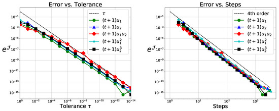
Figure 1. Verification of Theorem 2 using 4-th order schemes for the goal oriented adaptive method on Problem (33) for $k=-1$ and functionals $j(t,\mathit{u})$ as shown in the legend.

5.1.3. Method Comparison and Performance Tests

To compare DWR with the local error based methods, we use the Crank–Nicolson scheme and estimate local errors with Implicit Euler. Comparison is done in terms of computational efficiency (error vs. (wall-clock) runtime) and grid quality (error vs. number of timesteps). We consider $j(t,\mathit{u})=u_1$ for $k\in \{-1,-100\}$ and $j(t,\mathit{u})=u_2$ for $k=-1$. Results are shown in Figure 2.

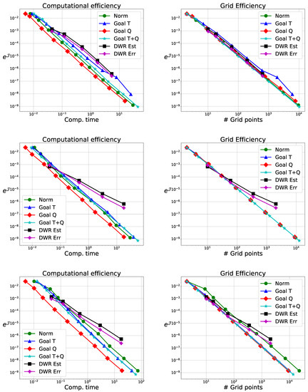
Figure 2. Performance comparison of the various methods for Problem (33). Top: $k=-1$ and $j(t,\mathit{u})=u_1$, center: $k=-1$ and $j(t,\mathit{u})=u_2$, bottom: $k=-100$ and $j(t,\mathit{u})=u_1$.

5.1.4. Discussion

Considering the global errors, we see DWR does not yield notably better grids, but it is significantly slower for small tolerances as it needs to solve adjoint problems.

In the case of $k=-1$ and $j(t,\mathit{u})=u_2$, we have comparable timesteps for all local error based methods, since the local error in the second component is dominant. These methods have grids of nearly identical quality and require the same computational effort.

For $j(t,\mathit{u})=u_1$, we get larger timesteps using the goal oriented method, particularly for $k=-100$. Due to the off-diagonal term in $\mathit{B}$, the flow map shifts errors from the second component, the zero set of j, to the first component. This leads to comparable performance for $k=-1$ and a performance gain for $k=-100$. While not immediately evident, for $k=-1$, we have $j(t,{\mathbf{\varphi }}_{-}(t,\mathit{u}(t)))=\frac{1}{2}{\mathtt{e}}^{-t}(t-1)$ and do not fulfill Equation (27), which is needed for convergence in the QoI. This does, however, not cause computational problems here, but we see notably worse performance when using only the time-integration error estimate.

Comparing the computational efficiency with the grid qualities, we see the goal oriented method using only the quadrature estimate has better performance results than other methods with the same grid quality. This is because we reuse values computed for ${\mathcal{J}}_h({\mathit{u}}_h)$.

5.2. Convection–Diffusion Equation

As a problem with a spatial component, we look at a linear convection-diffusion problem given by

$$\begin{array}{c}\hfill \begin{array}{cc}\hfill {\partial }_{t}u(t,\mathit{x})+a\mathit{v}·\nabla u(t,\mathit{x})-\gamma \Delta u(t,\mathit{x})=f(t,\mathit{x}),& (t,\mathit{x})\in [t_0,t_e]\times \Omega ,\hfill \\ \hfill u(t_0,\mathit{x})=u_0(\mathit{x}),& \mathit{x}\in \Omega \hfill \\ \hfill \nabla u·\mathbf{n}=-cu(t,\mathit{x}),& (t,\mathit{x})\in [t_0,t_e]\times \partial \Omega .\hfill \end{array}\end{array}$$

(34)

We want to model the case of having error build-up in the zero set of $j(t,u)$, which is transported into its image. For this, we consider the domain $\Omega =[0,3]\times [0,1]$. We choose a source term f with support ${\Omega }_f=[0.25,0.75]\times [0.25,0.75]$ and a spatially local QoI sufficiently far away in the downwind direction at ${\Omega }_{*}=[2.25,2.75]\times [0.25,0.75]$. For a visualization of the spatial domain, see Figure 3, for the time-domain we use $[t_0,t_e]=[0,6]$.

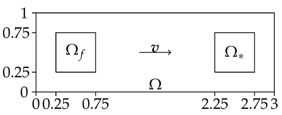
Figure 3. Geometry of $\Omega$ for the convection–diffusion Problem (34).

The QoI we consider is

$$\mathcal{J}(u)={\int }_{t_0}^{t_e}{\int }_{{\Omega }_{*}}\frac{u(t,\mathit{x})}{t_e-t_0}\mathrm{d}\mathit{x},$$

(35)

i.e., the average value, time and space, in ${\Omega }_{*}$. We use the source term

$$f(t,\mathit{x})=\left\{\begin{array}{cc}5t^3,\hfill & \mathit{x}\in {\Omega }_f\mathrm{and}t<1,\hfill \\ 5{(2-t)}^3,\hfill & \mathit{x}\in {\Omega }_f\mathrm{and}1\le t<2,\hfill \\ 0,\hfill & \mathit{x}\notin {\Omega }_f\mathrm{or}2\le t,\hfill \end{array}\right.$$

providing a spike-shaped build-up around $t=1$. The remaining parameters are $a=0.5$, $\gamma =0.01$, $c=0.15$, $\mathit{v}={(1,0)}^{\mathrm{T}}$, and $u_0(\mathit{x})=1+0.2sin(\pi x_1/3)sin(\pi x_2)$. We use as reference solution the result from the classic adaptive method with $\tau ={10}^{-8}$.

5.2.1. Discretization

For our convection–diffusion problem we have a weak solution in the space

$$V:=H^1(t_0,t_e;L^2(\Omega ))\cap L^2(t_0,t_e;H^1(\Omega )),$$

see [28]. We get the variational formulation

$$\underset{A(u,\varphi )}{\underbrace{{\int }_{\Omega }{\int }_{t_0}^{t_e}{u}_t\varphi +a(\mathit{v}·\nabla u)\varphi -\gamma \Delta u\varphi \mathrm{d}t+u(t_0)\varphi (t_0)\mathrm{d}\mathit{x}}}=\underset{F(\varphi )}{\underbrace{{\int }_{\Omega }{\int }_{t_0}^{t_e}f\varphi \mathrm{d}t+u_0\varphi (t_0)\mathrm{d}\mathit{x}}},\forall \varphi \in V.$$

By some standard reformulation we get the weak form

$${\int }_{t_0}^{t_e}{\int }_{\Omega }(u_t+a(\mathit{v}·\nabla u)-f)\varphi -\gamma \nabla u·\nabla \varphi \mathrm{d}\mathit{x}+\gamma c{\int }_{\partial \Omega }u\varphi \mathrm{d}s\mathrm{d}t={\int }_{\Omega }{u}_0\varphi (t_0)-u(t_0)\varphi (t_0)\mathrm{d}\mathit{x},\forall \varphi \in V.$$

We discretize time along the points $t_n$ with $I_n:=[t_n,t_{n+1}]$ and space by $2(3·32)·32=6144$ regular triangular cells K defining the finite element mesh. We define the global finite element space by

$$V_{h,k}=\{v\in L^{\infty }(t_0,t_e;H^1(\Omega )){:v(t,·)|}_{Q_K^n}\in Q^1(K),v(·,x){|}_{Q_K^n}\in P^q(I_n),\forall Q_K^n\},$$

where $P^q(I_n)$ is the space of polynomials on $I_n$ of degree up to q and $Q^1(K)$ the space of polynomials on K with partial degrees up to 1. The adjoint problem to Equations (34) and (35) is

$$\begin{array}{cc}\hfill -z_t(t,\mathit{x})-a\mathit{v}·\nabla z(t,\mathit{x})-\gamma \Delta z(t,\mathit{x})=\frac{1}{t_e-t_0}{|}_{{\Omega }_{*}},& (t,\mathit{x})\in [t_0,t_e]\times \Omega ,\hfill \\ \hfill z(t_e,\mathit{x})=0,& \mathit{x}\in \Omega ,\hfill \\ \hfill \nabla z(t,\mathit{x})·\mathit{n}=-\frac{a}{\gamma }z(t,\mathit{x})\mathit{v}·\mathit{n}-cz(t,\mathit{x}),& (t,\mathit{x})\in [t_0,t_e]\times \partial \Omega .\hfill \end{array}$$

5.2.2. DWR Estimate

We have the error in the QoI given by

$$e^{\mathcal{J}}=\left|{\int }_{t_0}^{t_e}{\int }_{\Omega }({(u_h)}_t+a(\mathit{v}·\nabla u_h)-\gamma \Delta u_h-f)(z-z_h)\mathrm{d}\mathit{x}\mathrm{d}t\right|,$$

where we approximate $z\approx z_h^{+}$ by a finer grid in time. Splitting this by timesteps gives

$$e^{\mathcal{J}}\lesssim \sum _{n=0}^{N-1}\left|{\int }_{t_n}^{t_{n+1}}\underset{=:R_z(t)}{\underbrace{{\int }_{\Omega }({(u_h)}_t+a(\mathit{v}·\nabla u_h)-\gamma \Delta u_h-f)(z_h^{+}-z_h)\mathrm{d}\mathit{x}}}\mathrm{d}t\right|.$$

We use the composite trapezoidal rule to get the error estimate

$$e^{\mathcal{J}}\lesssim {\eta }_h(u_h):=\sum _{n=0}^{N-1}\frac{\Delta t_n}{4}\left|R_z(t_n)+2R_z(t_n+\Delta t_n/2)+R_z(t_{n+1})\right|,$$

using linear interpolation for $u_h$ and $z_h$ in computing $R_z(t_n+\Delta t_n/2)$.

5.2.3. Method Comparison and Performance Tests

We use the same time-integration as in Section 5.1.3. The source term is in the zero set of $j(t,u)$ and due to convection $\mathcal{M}$ shifts build-up from ${\Omega }_f$ to ${\Omega }_{*}$. Thus, we expect the goal oriented method to perform poorly due to a huge error growth in the zero-set, which later becomes part of the error in the QoI.

5.2.4. Discussion

In Figure 4 (top), we observe the classical adaptive method performs well and the goal oriented adaptive methods, as expected, perform worse. There, timesteps are clearly too big for the given source term. Nevertheless, convergence in the QoI with $e^{\mathcal{J}}=\mathcal{O}(\tau )$ is observed, as predicted by Theorem 2. The DWR method is expensive but gives high quality grids. Here, we used it to only adapt in time.

Figure 4. Comparison of the various methods for the convection diffusion Problem (34) with QoI as in Equation (35). (Top): Performance for positive $\mathit{v}$. (Centre): Tolerance over error and chosen timesteps for $\tau ={10}^{-6}$ (positive $\mathit{v}$). (Bottom): Performance for negative $\mathit{v}$ and $t_e=3$.

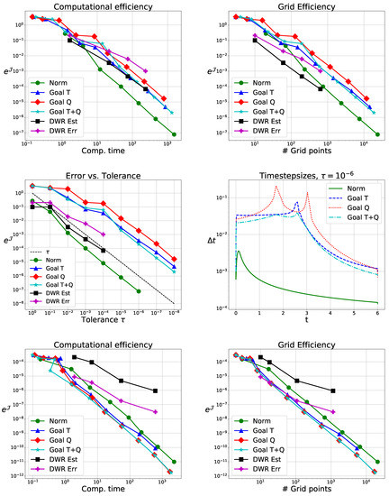
Changing the sign of the convection term, we expect good results for the goal oriented method, as the source term can be neglected. This is observed in Figure 4; bottom (reference solution with $\tau ={10}^{-9}$). The goal oriented methods perform better than the classical one. The DWR method performs notably worse than in the previous examples.

5.3. Thermal Fluid Structure Interaction

The previous examples were of academic nature, to demonstrate strength and weaknesses of the method, as predicted in Section 4.3. As a third test problem, we consider the coupling of two heat equations with different thermal conductivities and diffusivities. This models, for example, steel cooling with pressurized air. Furthermore, this example will show how the proposed method can be applied seamlessly in a partitioned approach. The model equations for this problem are

$$\begin{array}{cc}\hfill {\alpha }_m\frac{\partial u_m(t,\mathit{x})}{\partial t}-\nabla ·({\lambda }_m\nabla u_m(t,\mathit{x}))=0,& (t,\mathit{x})\in [t_0,t_e]\times {\Omega }_m,\hfill \\ \hfill u(t,\mathit{x})=0,& (t,\mathit{x})\in [t_0,t_e]\times {\Omega }_m\backslash \Gamma ,\hfill \\ \hfill u_1(t,\mathit{x})=u_2(t,\mathit{x}),{\lambda }_2\frac{\partial u_2(t,\mathit{x})}{\partial {\mathit{n}}_2}=-{\lambda }_1\frac{\partial u_1(t,\mathit{x})}{\partial {\mathit{n}}_1},& (t,\mathit{x})\in [t_0,t_e]\times \Gamma ,\hfill \\ \hfill u_m(t_0,\mathit{x})=u_m^0(\mathit{x}),& \mathit{x}\in {\Omega }_m,m=1,2.\hfill \end{array}$$

(36)

Our QoI is the time-averaged heat transfer over the interface $\Gamma$ and given by

$$\mathcal{J}(u)={\int }_{t_0}^{t_e}{\int }_{\Gamma }\frac{1}{t_e-t_0}{\lambda }_1\frac{\partial u_1(t,\mathit{x})}{\partial {\mathit{n}}_1}\mathrm{d}\mathit{x}\mathrm{d}t,$$

which in the discrete case is given by the finite difference

$${\mathcal{J}}_h(u_h)=\sum _{i=1}^{n-1}{u}_{\Gamma }^i-u_{1,\Gamma }^i,$$

where $u_{\Gamma }^i\approx u(1,i\Delta x)$ and $u_{1,\Gamma }^i\approx u(1-\Delta x,i\Delta x)$.

We consider the spatial domains ${\Omega }_1=[0,1]\times [0,1]$, ${\Omega }_2=[1,2]\times [0,1]$, $\Gamma ={\Omega }_1\cap {\Omega }_2$, and $[t_0,t_e]=[0,0.2]$. We use the initial conditions

$$u^0(x,y)=\left\{\begin{array}{cc}800sin{(\pi y)}^{2}sin(2\pi x),\hfill & x\le 0.5\hfill \\ 200sin{(\pi y)}^{2}sin(\pi (x-0.5)),\hfill & 0.5<x\le 1.5\hfill \\ 0,\hfill & \mathrm{else}\hfill \end{array}\right.,$$

(37)

see Figure 5, which also shows the geometry.

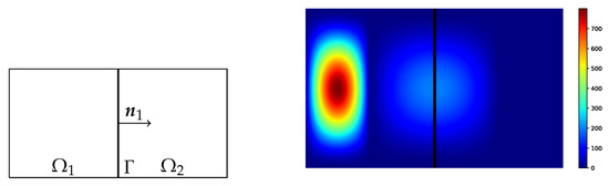
Figure 5. (Left): Geometry for the coupled heat problem. (Right): Initial condition (Equation (37)).

For time-integration we use SDIRK2, which is implicit with $(p,\widehat{p})=(2,1)$. To solve the problem arising from the so called transmission conditions (Equation (36)) on the interface $\Gamma$, we use the Dirichlet–Neumann iteration for each stage derivative of SDIRK2 [29]. We choose the parameters ${\alpha }_1=0.1,{\lambda }_1=0.01$ and ${\alpha }_2={\lambda }_2=1$. Based on the results of [30], this gives us a convergence rate of approximately ${\alpha }_1/{\alpha }_2=0.1$ for the Dirichlet–Neumann iteration for $\Delta t\to 0$.

Standard linear FE are used in space for both domains with identical triangular meshes for $\Delta x=1/81$. Details of the implementation of the discretization and methods can be found in [31].

For this problem, we use $\Delta t_0=\tau$. The reference solution is computed using the classical scheme with $\tau ={10}^{-6}$ and an absolute tolerance of ${10}^{-12}$ in the Dirichlet–Neumann iteration, where the numerical tests use an absolute tolerance of $\tau /100$.

5.3.1. Method Comparison and Performance Tests

Based on the results from the previous problems, we no longer consider the DWR method. While we specifically considered both grid quality and computational efficiency because of the DWR method, we now look only at grid quality, as these two performance measures are essentially identical here.

We chose $u^0$ and $t_e$ such that there is notable initial heat in the domain ${\Omega }_1$, but it has little relevance to the heat flux over the interface $\mathbf{\Gamma }$.

5.3.2. Discussion

As a result, the classical method will choose small timesteps to correctly resolve the diffusion process on the whole domain, effectively over-resolving the time-domain with respect to the error in the QoI. We expect larger timesteps for the goal-oriented methods with a higher computational efficiency. As seen in Figure 6, we have a gain in efficiency for larger tolerances by a factor larger than 10. For smaller tolerances, this factor is smaller.

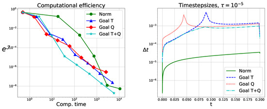
Figure 6. Comparison of the local error based adaptive methods for the coupled heat problem.

Furthermore, Figure 6 shows the timesteps for $\tau ={10}^{-5}$. There, we see upward cusps for the goal-oriented method when using only one error estimate, which are due to sign changes in the heat flux. These violate the controllability requirement (Equation (27)). For both the quadrature and time-integration error, there is no common zero. This guarantees convergence for $\tau \to 0$ and gives significantly better performance results.

6. Conclusions

Similar to previously proposed methods, we derived a simple and easy to implement goal oriented local error estimator. Implementation comes with little to no extra work and is well-suited for partitioned approaches for coupled systems.

For the resulting goal oriented adaptive method, we show convergence for the first time and its rates with respect to the error in the QoI. To obtain tolerance proportionality, sufficiently high order solutions in all quadrature evaluation points are needed. The proof is constructive and gives rise to a principle to formally show convergence for closely related stepsize controllers.

Performance of the goal oriented method deteriorates when local errors of underresolved processes accumulate in the zero set of the density function that later shift into its image. This can be the case for convection dominated problems, and one should then consider using the standard local error estimate. It is less problematic for dissipative problems, where slow and global processes dominate the error.

Numerical experiments designed to test these guidelines show them to work well, as well as confirming the results on convergence rates. The tests show that bad performance of the goal oriented method can be predicted and thus avoided. For dissipative test cases, the DWR method is notably more expensive and outperformed by the local error based method. The goal oriented adaptive method shows good performance in most cases and significant speedups in some.

Future Work

It would be interesting to test the proposed goal oriented method in the context of PDE-constrained optimization. There, one has to repeatedly solve a given PDE for varying parameters. This would be particularly interesting for non-gradient based optimization algorithms, where the proposed method could lead to considerable speedups for the optimization process as a whole.

Our analysis is based on a specific type of QoI. It is natural to try to extend our results to more general QoIs, for example, point-wise evaluations in time.

One could further generalize this work by using a density function $j_{\mathrm{est}}$ in error estimation, that is not the density function j from the QoI. This adds a degree of freedom in constructing the goal oriented method and can be used to overcome possible weaknesses, such as vanishing error estimates. This requires further testing and gives rise to the question on how to optimally choose $j_{\mathrm{est}}$.

References

- Helsen, M.M.; Van De Berg, W.J.; Van De Wal, R.S.; Van Den Broeke, M.R.; Oerlemans, J. Coupled regional climate-ice-sheet simulation shows limited Greenland ice loss during the Eemian. Clim. Past 2013, 9, 1773–1788. [Google Scholar] [CrossRef]
- Xudong, W.; Shen, W.Z.; Zhu, W.J.; Sørensen, J.N.; Jin, C. Shape optimization of wind turbine blades. Wind Energy 2009, 12, 781–803. [Google Scholar] [CrossRef]
- Funke, S.W.; Farrell, P.E.; Piggott, M.D. Tidal turbine array optimisation using the adjoint approach. Renew. Energy 2014, 63, 658–673, arXiv:1304.1768v1. [Google Scholar] [CrossRef]
- Becker, R.; Rannacher, R. An optimal control approach to a posteriori error estimation in finite element methods. Acta Numer. 2001, 10, 1–102. [Google Scholar] [CrossRef]
- Prudhomme, S. A Posteriori Error Estimates of Quantities of Interest. In Encyclopedia of Applied and Computational Mathematics; Springer: Berlin/Heidelberg, Germany, 2015; pp. 1–5. [Google Scholar]
- Meidner, D.; Richter, T. Goal-oriented error estimation for the fractional step theta scheme. Comput. Methods Appl. Math. 2014, 14, 203–230. [Google Scholar] [CrossRef]
- Meidner, D.; Richter, T. A posteriori error estimation for the fractional step theta discretization of the incompressible Navier-Stokes equations. Comput. Methods Appl. Mech. Eng. 2015, 288, 45–59. [Google Scholar] [CrossRef]
- Steiner, C.; Noelle, S. On adaptive timestepping for weakly instationary solutions of hyperbolic conservation laws via adjoint error control. Int. J. Numer. Methods Biomed. Eng. 2010, 26, 790–806. [Google Scholar] [CrossRef]
- Carey, V.; Estep, D.J.; Johansson, A.; Larson, M.G.; Tavener, S. Blockwise adaptivity for time dependent problems based on coarse scale adjoint solutions. SIAM J. Sci. Comput. 2010, 32, 2121–2145. [Google Scholar] [CrossRef]
- Jando, D. Efficient goal-oriented global error estimators for BDF methods using discrete adjoints. J. Comput. Appl. Math. 2017, 316, 195–212. [Google Scholar] [CrossRef]
- Hairer, E.; Nørsett, S.P.; Wanner, G. Solving Ordinary Differential Equations I; Springer: Berlin, Germany, 1993. [Google Scholar]
- Shampine, L.F. Numerical Solution of Ordinary Differential Equations; CRC Press: Boca Raton, FL, USA, 1994; Volume 4. [Google Scholar]
- Sandu, A. (Department of Computer Science, Virginia Tech, Blacksburg, VA, USA). Personal Communication, September 2018.
- Meisrimel, P.; Birken, P. On Goal Oriented Time Adaptivity using Local Error Estimates. PAMM 2017, 17, 849–850. [Google Scholar] [CrossRef]
- John, V.; Rang, J. Adaptive time step control for the incompressible Navier-Stokes equations. Comput. Methods Appl. Mech. Eng. 2010, 199, 514–524. [Google Scholar] [CrossRef]
- Turek, S. Efficient Solvers for Incompressible Flow Problems: An Algorithmic and Computational Approach, 6th ed.; Springer: Berlin/Heidelberg, Germany, 1999. [Google Scholar]
- Failer, L.; Wick, T. Adaptive Time-Step Control for Nonlinear Fluid-Structure Interaction. J. Comput. Phys. 2018, 366, 448–477. [Google Scholar] [CrossRef]
- Wick, T. Coupling fluid-structure interaction with phase-field fracture: algorithmic details. In Fluid-Structure Interaction: Modeling, Adaptive Discretizations and Solvers; Frei, S., Holm, B., Richter, T., Wick, T., Yang, H., Eds.; Radon Series 20; De Gruyter: Berlin, Germnay, 2017; pp. 1–37. [Google Scholar]
- Söderlind, G. Digital filters in adaptive time-stepping. ACM Trans. Math. Softw. 2003, 29, 1–26. [Google Scholar] [CrossRef]
- Bangerth, W.; Rannacher, R. Adaptive Finite Element Methods for Differential Equations; Birkhäuser: Basel, Switzerland, 2013. [Google Scholar]
- Griewank, A.; Walther, A. Algorithm 799: Revolve: An Implementation of Checkpointing for the Reverse or Adjoint Mode of Computational Differentiation. ACM Trans. Math. Softw. (TOMS) 2000, 26, 19–45. [Google Scholar] [CrossRef]
- Farrell, P.E.; Ham, D.A.; Funke, S.W.; Rognes, M.E. Automated derivation of the adjoint of high-level transient finite element programs. SIAM J. Sci. Comput. 2013, 35, C369–C393. [Google Scholar] [CrossRef]
- Shampine, L.F. The step sizes used by one-step codes for ODEs. Appl. Numer. Math. 1985, 1, 95–106. [Google Scholar] [CrossRef]
- Söderlind, G. The logarithmic norm. History and modern theory. BIT Numer. Math. 2006, 46, 631–652. [Google Scholar] [CrossRef]
- Gear, C.W. Numerical Initial Value Problems in Ordinary Differential Equations; Prentice Hall PTR: Upper Saddle River, NJ, USA, 1971. [Google Scholar]
- Logg, A.; Mardal, K.A.; Wells, G. Automated Solution of Differential Equations by the Finite Element Method: The FEniCS Book; Springer: Berlin/Heidelberg, Germany, 2012; Volume 84. [Google Scholar]
- Meisrimel, P. Available online: https://github.com/PeterMeisrimel/goal_oriented (accessed on 30 April 2020).
- Renardy, M.; Rogers, R.C. An Introduction to Partial Differential Equations; Springer: Berlin/Heidelberg, Germany, 2006; Volume 13. [Google Scholar]
- Birken, P.; Quint, K.J.; Hartmann, S.; Meister, A. A time-adaptive fluid-structure interaction method for thermal coupling. Comput. Vis. Sci. 2010, 13, 331–340. [Google Scholar] [CrossRef]
- Monge, A.; Birken, P. On the convergence rate of the Dirichlet-Neumann iteration for unsteady thermal fluid-structure interaction. Comput. Mech. 2018, 62, 525–541. [Google Scholar] [CrossRef]
- Monge, A. The Dirichlet-Neumann Iteration for Unsteady Thermal Fluid Structure Interaction. Licentiate Thesis, Lund University, Lund, Sweden, 2016. [Google Scholar]
© 2020 by the authors. Licensee MDPI, Basel, Switzerland. This article is an open access article distributed under the terms and conditions of the Creative Commons Attribution (CC BY) license (http://creativecommons.org/licenses/by/4.0/).