An Enhanced Lightning Attachment Procedure Optimization Algorithm

Abstract

To overcome the shortcomings of the lightning attachment procedure optimization (LAPO) algorithm, such as premature convergence and slow convergence speed, an enhanced lightning attachment procedure optimization (ELAPO) algorithm was proposed in this paper. In the downward leader movement, the idea of differential evolution was introduced to speed up population convergence; in the upward leader movement, by superimposing vectors pointing to the average individual, the individual updating mode was modified to change the direction of individual evolution, avoid falling into local optimum, and carry out a more fine local information search; in the performance enhancement stage, opposition-based learning (OBL) was used to replace the worst individuals, improve the convergence rate of population, and increase the global exploration capability. Finally, 16 typical benchmark functions in CEC2005 are used to carry out simulation experiments with LAPO algorithm, four improved algorithms, and ELAPO. Experimental results showed that ELAPO obtained the better convergence velocity and optimization accuracy.

1. Introduction

The optimization problems in engineering field can be expressed by mathematical models and solved by mathematical or numerical methods. With the development of science and technology, more and more engineering optimization problems are developing in the direction of large-scale, multi-peak, non-linear, and complex. It is difficult to solve them by traditional numerical methods. Meta-heuristic algorithm is an algorithm designed to solve approximate large-scale difficult optimization problems without deep adaptation to each problem. In recent decades, in order to overcome the shortcomings of slow computation speed and low reliability of traditional numerical methods in solving engineering problems, researchers have proposed a large number of meta-heuristic algorithms [1,2,3], which are widely used to solve complex problems in industries and services, from planning to production management and even engineering [4,5,6,7,8].

Meta-heuristic algorithms have some differences in the optimization mechanism, but they are similar in the optimization process. They are all “neighborhood search” structures. The algorithm starts from an initial solution (or a group of) and generates several neighborhood solutions through the neighborhood function under the control of the key parameters of the algorithm. It updates the current state according to the acceptance criteria (deterministic, probabilistic, or chaotic) and then adjusts the key parameters according to the key parameters modification criteria. Repeat the above search steps until the convergence criteria of the algorithm are satisfied, and finally the optimization results of the problem are obtained. Meta-heuristic optimization algorithms can be divided into evolutionary heuristic algorithm, group heuristic algorithm, and physical heuristic algorithm according to different inspiration sources.

Evolutionary heuristic algorithms are algorithms inspired by biological evolution in nature. Genetic algorithm [9] is the earliest and representative evolutionary heuristic algorithm, which inspired by Darwin’s evolutionary theory, it updates the individual through three processes: selection, crossover, and mutation. Differential evolutionary algorithm (DE) [10], evolution strategy (ES) [11], genetic programming (GP) [12], covariance-matrix adaptation evolution strategy [13], and biogeography-based optimizer (BBO) [14] are other methods under this category.

Group heuristic algorithms simulate the population behavior of insects, cattle, birds, and fish. These groups seek food in a cooperative way. Each member of the population constantly changes the direction of search by learning from his own experience and the experience of other members. The prominent feature of group heuristic algorithm is to use individuals in the population to search cooperatively, so as to find the optimal solution in the solution space. Particle swarm optimization (PSO) is the most representative algorithm. It is inspired by the foraging behavior of birds. For each individual, the position is updated according to its current speed, optimal position, and global optimal position [15]. The other methods that could be classified in this group are the artificial bee colony algorithm (ABC) [16], monkey search algorithm (MSA) [17], firefly algorithm (FA) [18], grey wolf optimization algorithm (GWO) [19], moth-flame optimization algorithm (MFO) [20], and so on.

The physical heuristic evolutionary algorithms are inspired by physical phenomena in nature and in these methods, the physical rules were used to update the solutions in each iteration. For example, in 2011, inspired by the spiral motion of galaxies in the universe, Shah-Hosseini H proposed a galaxy-based search algorithm (GbSA) [21]; in 2012, inspired by Newton’s second law, Rashedi E and others proposed gravitational search algorithms (GSA) [22]; in the same year, Kaveh A et al. were inspired by the refraction of light and proposed the ray optimization algorithms (RO) [23]; Hatamlou proposed a heuristic algorithm, which was named the black hole algorithms (BH) based on the black hole phenomenon in 2013 [24]; in 2016, inspired by the evaporation of water molecules on solid surfaces, Kaveh A et al. proposed an algorithm named the water evaporation optimization algorithm (WEO) [25].

Based on the No-Free-Lunch theorem, it cannot be claimed that optimization methods could solve all the problems. In order to solve a wider range of optimization problems, a new method has been introduced, in 2017, Iranian scholar A. Foroughi Nematollahi and others, inspired by the nature of lightning attachment process, proposed the lightning attachment procedure optimization (LAPO) [26]. It is compared with nine algorithms, such as the particle swarm optimization (PSO), differential evolution (DE), gray wolf optimizer (GWO), and cuckoo search algorithms (CSA), on four sets of 29 standard test functions. The results show that the LAPO algorithm has obvious advantages in convergence speed and accuracy, but similar to other swarm intelligence optimization algorithms, the LAPO algorithm also has some shortcomings, such as slow convergence speed in the middle and later stages of the evolutionary search, and easy to fall into local optimum when solving high-dimensional and multi-peak problems. Since the LAPO algorithm was put forward shortly, it has not been paid enough attention by scholars in various fields, and the theoretical system of the LAPO algorithm is still far from perfect. In order to further improve the optimization performance of the LAPO algorithm, an enhanced lightning attachment procedure optimization algorithm (ELAPO) is proposed in this paper. The downward leader movement combines the renewal mechanism of differential evolution algorithm with the original renewal mechanism, and introduces the optimal individuals in the population to participate in the evolution. Speeds up the convergence rate of the population through the differential evolution mechanism on the basis of distinguishing the better and worse individuals in the original algorithm. The upward leader movement changes the direction and step size of individual learning, and makes the individual jump out of the local optimum. In the process of performance improvement, the dynamic opposition-based learning (OBL) [27] method is used to replace the original update operation. Experiments show that this method can effectively improve the convergence speed of the algorithm. At the same time, to test the ELAPO performance, we tested 16 benchmark functions, and compared the experimental results with LAPO and four improved optimization algorithms results.

The rest of this paper is organized as follows. Section 2 briefly introduces the principle and process of the standard LAPO algorithm. Section 3 describes the ELAPO algorithm combined with differential evolution and opposition-based learning in detail. The experiments and results analysis are reported in Section 4. Section 5 concludes this paper.

2. The Lightning Attachment Procedure Optimization Algorithm

In nature, there are a large number of positive charges on the upper surface of the thunderstorm clouds, and a large number of negative charges and a small number of positive charges on the lower surface. As the charge increases, the edge of the cloud breaks down, creating a trapezoidal downward pilot that gradually extends to the ground. Affected by this, the space electric field near ground objects such as lightning rods, conductors, poles, and towers will continue to increase. To a certain extent, it will lead to an upward return stroke through the ionization channel opened by the downward trapezoidal pilot, that is, from the ground to the bottom of the cloud, forming a flash-over. When three or four flash-overs occur, there will be a gap breakdown, accompanied by pulse discharge, forming thunder and lightning. In this process, many pulsed discharges were carried out. Since each pulse discharge consumes a large amount of charge accumulated in thunderstorm clouds, the discharge process will become weaker and weaker until the charge reserve in thunderstorm clouds is exhausted, the pulse discharge can stop. The point at which the breakdown discharge may occur is defined as the test point, and the point at which charge depletion occurs is called the strike point.

To simulate the process of lightning formation, the LAPO abstracts the test points between the cloud and ground as individuals, the electric field corresponding to the test points as fitness, and the downward trapezoidal pilot, upward return stroke and pulse discharge processes of lightning as three evolutionary operations, namely downward leader movement, upward leader movement, and branch fading. Branch decline runs through the other two evolutionary processes and gradually guides individual evolution. The key operation details of the LAPO algorithm are as follows:

2.1. Initialize the Population

Population is the set of all decision variables in the definition domain of optimization problems. In the LAPO algorithm, individuals in the population represent test points where breakdown may occur, and each individual in the population can serve as a starting point for downward or upward leaders. Suppose that the upper limit of the definition domain is ub and the lower limit is lb. Individuals are generated according to formula (1) to form the initial population.

$$X_{i,j}^t=lb+\left(ub-lb\right)\times rand.$$

(1)

In the formula $X_{i,j}^t$ represents the j-dimensional (j = 1, 2, 3, ……, D) particle of the i-th (i = 1, 2, 3, ……, NP) individual of the population in the t-th generation. In the initialization stage, t = 0, rand is a random number between [0,1].

2.2. Downward Leader Movement

During lightning downward leader movement, all test points are considered as potential next jump points for a particular test point. Since lightning has random behavior, individual j ($i\ne j$) is randomly selected in the population for test point i. If the electric field of j is higher than the average value, that is, the fitness of j is better than F_ave, which is the fitness of the average individual $X_{ave}=\frac{1}{NP}{\displaystyle \sum _{i=1}^{NP}{X}_i}$, lightning will jump to that point, otherwise lightning will move in another direction, as shown in formula (2):

$$X_{inew}^t=\{\begin{array}{l}{X}_i^t+rand\times \left(X_{ave}+rand\times \left(X_j^t\right)\right),F_j^t<F_{ave}\\ X_i^t-rand\times \left(X_{ave}+rand\times \left(X_j^t\right)\right),else\end{array}.$$

(2)

In the formula, rand is a random number between [0,1], and j is a randomly selected individual, which is not equal to i.

2.3. Upward Leader Movement

In the process of upward leader movement, all particles move upward along the charge channel opened by the downward leader and distribute exponentially in the channel. The updating mode of each particle’s position is shown in formula (3).

$$X_{inew}=X_i+rand\times S\times \left(X_{min}-X_{max}\right).$$

(3)

Among them, X_min and X_max are represented as the best and the worst individual of the current population respectively, and the exponential factor S is shown in formula (4).

$$S=1-\left(\frac{t}{t_{max}}\right)\times exp\left(-\frac{t}{t_{max}}\right).$$

(4)

t and t_max represent the number of iterations and the maximum number of iterations respectively.

2.4. Branch Fading

In the whole process of lightning formation, if the electric field of the new test point is higher than that of the previous point, the lightning branch will be generated and the pulse discharge will continue. On the contrary, the branch will disappear and the lightning formation will stop.

The LAPO algorithm simulates the above-mentioned fading process and chooses individuals according to formula (5).

$$X_i^{t+1}=\{\begin{array}{l}{X}_{inew}^t{F}_{inew}^t<F_i^t\\ X_i^{t}otherwise\end{array}.$$

(5)

The above two parts of the evolutionary operations, the downward leader movement and the upward leader movement, are selected and updated by branch fading, and for the individuals beyond the boundary generated in the downward and upward leader searches, the boundary absorption method is used, that is, the individuals beyond the boundary are placed on the boundary.

2.5. Enhancement of the Performance

In order to improve the performance of the algorithm, the average of the whole population was calculated and the fitness of the average solution was obtained in each generation. If the fitness of the worst individual was worse than the fitness of the average individual, the worst individual was replaced by the average solution.

In summary, LAPO performs the enhancement of the performance, the downward leader movement, and the upward leader movement in turn in each iteration, and each evolutionary process is accompanied by branch fading and boundary value processing, as shown in Figure 1.

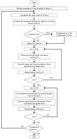
Figure 1. Flow chart of the lightning attachment procedure optimization (LAPO) algorithm.

3. The Enhanced Lightning Attachment Procedure Optimization Algorithm

To further improve the convergence accuracy and speed of the LAPO algorithm, a lightning attachment procedure optimization algorithm based on combined differential learning and opposition-based learning was proposed.

3.1. Improved Downward Leader Movement

In the downward leader movement of the LAPO algorithm, the individual updates according to formula (2). After an in-depth analysis, it was found that the updating method had the following defects:

Firstly, since individual i is not directly related to the evolutionary information of individual j and the average individual, it seems unreasonable to determine the updating mode of individual i based solely on the fitness relationship between individual j and the average individual.

Secondly, because of the multiplication of individual j and rand, the evolution of each individual is more dependent on the average individual. With the evolution, each individual will gather near the average individual, that is to say, the overall population diversity maintenance ability of the algorithm is not good and easy to fall into local optimum.

Thirdly, only one random individual is selected to learn from the average individual and the current individual, which does not guarantee the “best selection”. If the selected individual is the worst individual or the poorer individual, it will affect the evolution speed of the downward leader.

In view of this, this paper improves formula (2), as shown in formula (6).

$$X_{inew}^t=\{\begin{array}{l}{X}_i^t+rand\times \left(X_{ave}-X_j^t\right)+rand\times (X_{best}-X_i^t),F_i^t<F_{ave}\\ X_{ave}-rand\times \left(X_i^t-X_j^t\right)+rand\times (X_{best}-X_{ave}),F_i^t>F_{ave}\end{array}.$$

(6)

In the formula, $X_j^t$ is a randomly selected particle different from individual i, X_best represents the best individual in the current population, X_ave and F_ave are represented as the average individual and the fitness value of the average individual respectively.

As can be seen from formula (6), it has the following advantages:

Firstly, we regard individuals whose fitness value was better than the average fitness value as better individuals. For these individuals, they used themselves as base vectors to search around themselves. For the other solutions whose evolutionary information was not good enough, they used the central individual as base vectors to update and search around the average individuals. Obviously, compared with the LAPO algorithm, which only searches near the individual itself, the improved update method converged faster.

Secondly, compared with LAPO’s over-learning mode to the average individual, the proposed method integrated the individual j, the average individual, and the optimal individual, and introduced more combinations to enable the particles to obtain more local information, which was more conducive to maintaining the diversity of the population.

Thirdly, compared with the original update method, formula (6) refers to the update strategy of differential evolution algorithm, by adding two differential vectors to control the directive of evolution, avoiding over-learning to a particle and falling into local optimum, and removing the step factor rand before individual j in the original LAPO algorithm, thus avoiding the blindness of random step size, and individual j directly participates in the evolution process, which further accelerated the convergence speed of the algorithm.

Figure 2 takes the better individuals as an example to further describe the downward leader’s update strategy.

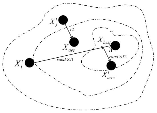
Figure 2. Diagram of the better individual renewal.

Take individual i as an example, if it is a better one, individual i adds the difference vector $X_{best}-X_i^t$, which is from individual $X_i^t$ to the best individual, close to the search area where the optimal individual is located, and then adds the difference vector $X_{ave}-X_j^t$ which is from individual j to the average individual, reach to $X_{inew}^t$. Since the j individual is randomly selected and the direction of the second difference vector is randomly generated, the current individuals can get more evolutionary directions and traverse the search interval where the excellent individuals are located more quickly.

3.2. Improvement of Upward Leader Movement

It can be seen from formula (4) that in the upward leader movement of LAPO, individuals are updated by learning from the best and worst individuals. As we all know, the worst individual carries relatively less information for evolution, there is a low probability of producing excellent individuals through them, which results in ineffective search and reduces the convergence speed of the algorithm.

Since the average individual contains evolutionary information of all individuals to some extent. Using average individuals instead of the worst individual to participate in evolution will inevitably increase the probability of obtaining better individuals and maintain the diversity of the population while improving the convergence rate. To this end, the updated formula of the upward leader, formula (4), is adjusted as follows:

$$X_{inew}=X_i+rand\times S\times \left(X_{ave}-X_{min}\right).$$

(7)

Combining formula (5), comparison formula (4), and formula (7), we can find that: In the early stage of evolution, S value is relatively large, and the proportion of learning results from other individuals is relatively large, while the average individual is much better than the worst one, and carries more information conducive to evolution, so learning from $X_{ave}-X_{min}$ is obviously faster than learning from $X_{min}-X_{max}$, and as evolution proceeds, each solution tends to be optimal, the range of $X_{ave}-X_{min}$ is obviously smaller than $X_{min}-X_{max}$, with the value of S decreases. That is to say, formula (7) has a relatively small search range, which is more conducive to the fine search near itself and improves the convergence accuracy of the algorithm. Moreover, $X_{ave}-X_{min}$ is a vector pointing to the average individual, which can effectively jump out of the local optimum by superposition it.

3.3. The Improved Enhancement Performance

The original algorithm updates the worst individual in each generation by comparing the fitness values of the newly generated average individual with the worst individual in the population and retaining the better one of them. According to the analysis of the experimental results and formulas, this operation can increase the convergence speed of the algorithm to a certain extent, but there is still room to improve its convergence speed.

Literature [27] points out that the opposition-based learning (OBL) of a particle is usually better than that of the original particle, so the probability of the average particle after the OBL is better than that of the original average individual. It is possible that the average individual after the OBL will take part in the evolution instead of the worst individual, which will lead to a faster convergence rate. In order to further accelerate the convergence speed of the algorithm, an improved opposition-based learning strategy as shown in formula (8) was adopted.

$$X_{ij}^{*}\left(t\right)=k\left(a_j\left(t\right)+b_j\left(t\right)\right)-X_{ij}^t,a_j(t)=min(X_{ij}(t)),b_j(t)=max(X_{ij}(t)),$$

(8)

where $X_{ij}^t$ represents the component of the first solution on the j-dimension, $X_{ij}^{*}\left(t\right)$ is its corresponding reverse solution, $a_j(t)$, $b_j(t)$ are the minimum and maximum values of the current search interval on the j-dimension, $i=1,2,\dots ,NP,j=1,2,\dots D$. The learning strategies obtained by different values of k are also different. Three strategies, k = 0.5, 1, and rand, are given in [27]. To verify the effectiveness of the improved strategy, the dynamic opposition-based learning strategy LAPO algorithm combined with k = 0.5, 1, rand, and the original LAPO algorithm were compared when the number of iterations was set to 500 generations. Experiments were carried out on typical single-peak function Sphere and multi-peak function Ackley, respectively. The results are shown in Figure 3, which show that for LAPO, when k = 0.5 and k = rand, the dynamic opposition-based learning strategy converged faster than the original algorithm, where k = rand had a relatively faster convergence rate. In order to improve the convergence speed of the algorithm, the formula (9) with k = rand was used to update the worst particle in this paper.

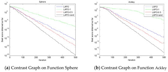
Figure 3. The comparison of LAPO and LAPO combined with opposition-based learning (OBL).

3.4. The Pseudo Code of the ELAPO Algorithm

Initialize the first population of test points randomly in the specific range

Calculate the fitness of test points

while the end criterion is not achieved

Set the test point with the worst fitness as Xw

for j = 1:D

$\begin{array}{l}a(j)=\min (X(:,j))\\ b(j)=\max (X(:,j))\\ X_{w\_new}(t)=rand*(a_j(t)+b_j(t))-X_{ave}(t)\end{array}$

end

if the fitness of $X_{w\_new}$ is better than the fitness of Xw

$\begin{array}{l}{X}_w=X_{w\_new}\\ F_w=F_{w\_new}\end{array}$

end

Obtain Xave which is the mean value of all the test points

Calculate the fitness of Xave as Fave

for i = 1:NP (each test point)

Select $X_j^t$ randomly which is not equal to $X_i^t$

Set the test point with the best fitness as $X_{best}^t$

for j = 1:D (number of variables)

Update the variables of $X_i^t$ based on Equation (6), as $X_{inew}^t$

Check the boundary. If the particle exceeds the boundary value, it is generated randomly within the boundary.

end

Calculate the fitness of $X_{inew}^t$

if the fitness of $X_{inew}^t$ is better than $X_i^t$

$X_i^t=X_{inew}^t$

end

end

for i = 1:NP (each test point)

for j = 1:D (number of variables)

Update the variables of $X_i^t$ based on Equation (8) as $X_{i\_new}^t$

Check the boundary. If the particle exceeds the boundary value, it is generated randomly within the boundary.

end

Calculation the fitness of $X_{i\_new}^t$

if the fitness of $X_{i\_new}^t$ is better than $X_i^t$

$X_i^t=X_{i\_new}^t$

end

end

XBEST = the test point with the best fitness

FBEST = the best fitness

end

return XBEST, FBEST

4. Analysis of the Simulation Results

In order to test the performance of the proposed ELAPO, a series of experiments were carried out in this section. All experiments were implemented on CPU: Intel (R) Core (TM) i5-4200H, 4G memory, and 2.8GHz main frequency computer. The program was implemented in the language of Matlab R2014a.

The experiment selected 16 benchmark functions in CEC2005 [28]. Among them, f1–f8 were unimode functions, f9–f16 were multimodal functions, the dimensions of the test functions from f1 to f14 were all set in 30 dimensions, and the dimensions of the test functions f15 and f16 were set in two dimensions, the specific functions are shown in Table 1.

Table 1. Test Functions.

Name	Function	Range	Optimal
f1 sumPower	$f\left(x\right)={\displaystyle \sum _{i=1}^D{\left|x_i\right|}^{\left(i+1\right)}}$	[−1, 1]	0
f2 Sphere	$f\left(x\right)={\displaystyle \sum _{i=1}^D{x}_i{}^2}$	[−100, 100]	0
f3 SumSquares	$f\left(x\right)={\displaystyle \sum _{i=1}^{D}i{x}_i^2}$	[−10, 10]	0
f4 Step	$f\left(x\right)={\displaystyle \sum _{i=1}^D{\left(x_i+0.5\right)}^2}$	[−1.28, 1.28]	0
f5 Schwefel 2.22	$f\left(x\right)={\displaystyle \sum _{i=1}^D\left|x_i\right|+{\displaystyle {\prod }_{i=1}^D\left|x_i\right|}}$	[−10, 10]	0
f6 Schwefel 1.2	$f\left(x\right)={\displaystyle \sum _{i=1}^D{\left({\displaystyle \sum _{j=1}^i{x}_j}\right)}^2}$	[−100, 100]	0
f7 Schwefel2.21	$f\left(x\right)=\underset{i=1}{\overset{D}{\max }}\left\{\left|x_i\right|\right\}$	[−100, 100]	0
f8 Schwefel1.2 with Noise	$f\left(x\right)=\left({{\displaystyle \sum _{i=1}^D\left({\displaystyle \sum _{j=1}^i{x}_j}\right)}}^2\right)\times \left(1+0.4\left|N\left(0,1\right)\right|\right)$	[−100, 100]	0
f9 Rastrigin	$f\left(x\right)={\displaystyle \sum _{i=1}^D\left(x_i^2-10\cos \left(2\pi x_i\right)+10\right)}$	[−5.12, 5.12]	0
f10 Shifted Rotated Rastrigin’s	$f\left(x\right)={{\displaystyle \sum _{i=1}^D\left({10}^{\frac{i-1}{D-1}}{x}_i\right)}}^2-10\cos (2\pi {10}^{\frac{i}{D-1}}{x}_i)+10$	[−5.12, 5.12]	0
f11 Griewank	$f\left(x\right)=\frac{1}{4000}\left({\displaystyle \sum _{i=1}^D{\left(x_i-100\right)}^2}\right)-\left({\displaystyle {\prod }_{i=1}^D\cos \left(\frac{x_i-100}{\sqrt{i}}\right)}\right)+1$	[−600, 600]	0
f12 Ackley	$f\left(x\right)=-20\exp \left(-0.2\sqrt{\frac{1}{n}{\displaystyle \sum _{i=1}^D{x}_i^2}}\right)-\exp \left(\frac{1}{n}{\displaystyle \sum _{i=1}^D\cos \left(2\pi x_i\right)}\right)+20+e$	[−32, 32]	0
f13 Weierstrass	$\begin{array}{l}f\left(x\right)={\displaystyle \sum _{i=1}^D\left({\displaystyle \sum _{k=0}^{k\max }\left[a^k\cos \left(2\pi b^k\left(z_i+0.5\right)\right)\right]}\right)-D{\displaystyle \sum _{k=0}^{k\max }\left[a^k\cos \left(2\pi b^k\cdot 0.5\right)\right]}}\\ a=0.5,b=3,k\max =20\end{array}$	[−0.5, 0.5]	0
f14 Himmelblau	$f(x)=\frac{1}{D}{\displaystyle {\sum }_{i=1}^D\left[x_i^4-16x_i^2+5x_i\right]}$	[−5, 5]	−78.3323
f15 Cross-in-tray	$f(x)=-0.0001{(\left|\sin (x_1)\sin (x_2)\exp \left(\left|100-\frac{\sqrt{x_1^2+x_2^2}}{\pi }\right|\right)\right|+1)}^{0.1}$	[−10, 10]	−2.0626
f16 Six-hump Camel	$f(x)=(4-2.1x_1^2+\frac{x_1^4}{3})x_1^2+x_1{x}_2+(-4+4x_2^2)x_2^2$	[−5.12, 5.12]	−1.0316

In order to further validate the advantages of ELAPO, the ELAPO algorithm was compared with the basic LAPO algorithm and the other four algorithms that have better optimization results in recent years, including: All-dimension neighborhood based particle swarm optimization with randomly selected neighbors (ADN-RSN-PSO) [29], enhanced artificial bee colony algorithms with adaptive differential operators (ABCADE) [30], an optimization algorithm for teaching and learning based on hybrid learning strategies (DSTLBO) [31], and a self-adaptive differential evolution algorithm with improved mutation strategy (IMSaDE) [32].

During the experiment, the parameters of the contrast algorithm were set as those in the literature. Except the number of population and the maximum number of function evaluations LAPO and DSTLBO did not involve any parameters. For this reason, Table 2 gives the parameter settings of other algorithms, all from the original literature.

Table 2. Arithmetic parameter settings.

Algorithms	Parameter
ADN-RSN-PSO	W = 0.7298, c1 = c2 = 2.05
ABCADE	SN = 50, limit = 200, m = 5, n = 10, c 1 = 0.9, c 2 = 0.999
IMSaDE	NEP = 7([0.1,0.3]*NP), ST = 3, CRl = 0.3, Cru = 1, Fl = 0.1, Fu = 0.9

In order to ensure fairness, the population number of each algorithm was 30, and the maximum number of function evaluations was 90,000. In order to avoid the harmful effect of the randomness of a single operation, each algorithm was run 30 times independently for each test function and recorded the maximum, average, minimum, variance of 30 experimental results, and the success rate of reaching the appointed precision and recorded Friedman ranking based on the average. The appointed precision was 10⁻¹⁰ for the benchmark functions whose optimal was 0, for the benchmark functions f14, f15, and f16 whose optimal was not equal to 0, the appointed precision was −78, −1.8, and −0.8 respectively. The statistical results are shown in Table 3.

Table 3. Convergence accuracy.

Function	Statistic	ADN-RSN-PSO	ABCADE	DSTLBO	IMSaDE	LAPO	ELAPO
f1	Min	1.9433 × 105	1.0604 × 10−122	0	9.1175 × 10−190	1.2787 × 10−140	0
	Mean	7.0621 × 10−3	5.0305 × 10−96	0	8.4357 × 10−171	1.4429 × 10−131	0
	Max	6.0864 × 10−2	1.5085 × 10−94	0	8.5523 × 10−170	3.7225 × 10−130	0
	Std	1.3886 × 10−2	2.7540 × 10−95	0	0	6.7837 × 10−131	0
	Robustness	0	100	100	100	100	100
	Rank	6	5	1.5	3	4	1.5
f2	Min	2.7340 × 10−9	6.1134 × 10−49	0	5.6607 × 10−95	1.3390 × 10−36	0
	Mean	4.5246 × 10−1	4.3991 × 10−42	2.4682 × 10−318	4.4691 × 10−88	1.2060 × 10−33	0
	Max	8.1548	6.9662 × 10−41	7.2645 × 10−317	4.8224 × 10−87	1.3582 × 10−32	0
	Std	1.5287	1.3292 × 10−41	0	1.2051 × 10−87	3.0653 × 10−33	0
	Robustness	0	100	100	100	100	100
	Rank	6	4	2	3	5	1
f3	Min	2.0553× 10−13	2.9427× 10−51	0	2.0072 × 10−95	1.1679 × 10−38	0
	Mean	2.5192	1.1781× 10−41	1.1660 × 10−321	1.1548 × 10−88	1.4772 × 10−33	0
	Max	4.9549 × 101	2.7244× 10−40	3.4760 × 10−320	3.4405 × 10−87	2.4542 × 10−32	0
	Std	9.134	5.0461× 10−41	0	6.2801 × 10−88	4.8781 × 10−33	0
	Robustness	10	100	100	100	100	100
	Rank	6	4	2	3	5	1
f4	Min	3.3295	0	4.2081	3.0815 × 10−33	2.0431 × 10−17	0
	Mean	5.6636	5.9986 × 10−32	5.476	1.1884 × 10−31	2.8720 × 10−16	1.0812 × 10−29
	Max	7.5679	8.0735 × 10−31	7.0288	1.5068 × 10−30	1.4498 × 10−15	4.2786 × 10−29
	Std	1.1575	1.4892 × 10−31	8.6427 × 10−1	2.7273 × 10−31	3.6114 × 10−16	1.7057 × 10−29
	Robustness	0	100	0	100	100	100
	Rank	6	1	5	2	4	3
f5	Min	5.2882 × 10−5	4.7392 × 10−32	5.7955 × 10−169	6.2444 × 10−53	5.1613 × 10−21	2.2875 × 10−175
	Mean	2.1283	2.9518 × 10−25	1.8017 × 10−162	2.9148 × 10−49	1.8239 × 10−19	7.2628 × 10−171
	Max	1.4320 × 101	5.0681 × 10−24	2.3000 × 10−161	3.1393 × 10−48	1.0955 × 10−18	1.5612 × 10−169
	Std	3.6429	9.9107 × 10−25	5.8809 × 10−162	8.1886 × 10−49	2.5217 × 10−19	0
	Robustness	0	100	100	100	100	100
	Rank	6	4	2	3	5	1
f6	Min	7.9614 × 10−11	4.9825 × 10−1	0	1.7910 × 10−13	3.6024 × 10−5	2.0577 × 10−204
	Mean	3.6063 × 101	2.1321 × 101	1.4778 × 10−317	2.2465 × 10−9	2.7988 × 10−4	3.8434 × 10−188
	Max	9.1658 × 102	1.0491 × 102	4.4236 × 10−316	6.6102 × 10−8	8.6964 × 10−4	1.1172 × 10−186
	Std	1.6698 × 102	2.3468 × 101	0	1.2061 × 10−8	2.1707 × 10−4	0
	Robustness	3.33	0	100	83.33	0	100
	Rank	6	5	1	3	4	2
f7	Min	1.4991 × 10−5	5.4163	5.0526 × 10−162	1.9698 × 10−2	1.1755 × 10−21	1.4981 × 10−122
	Mean	2.2665 × 10−1	1.2694 × 101	9.8249 × 10−155	1.7505 × 10−1	1.5051 × 10−19	2.1015 × 10−116
	Max	2.6331	2.1428 × 101	1.5939 × 10−153	5.8210 × 10−1	1.4967 × 10−18	3.4242 × 10−115
	Std	5.3499 × 10−1	3.9118	3.6036 × 10−154	1.4560 × 10−1	2.8717 × 10−19	6.6285 × 10−116
	Robustness	0	0	100	0	100	100
	Rank	6	5	1	4	3	2
f8	Min	9.1385 × 10−7	3.7190 × 10−13	1.9123 × 10−315	4.2590 × 10−51	7.2925 × 10−18	1.5064 × 10−298
	Mean	4.2904 × 102	6.4605 × 10−6	4.1842 × 10−298	6.1752 × 10−30	7.6451 × 10−17	1.7716 × 10−288
	Max	4.1982 × 103	7.5741 × 10−5	7.4227 × 10−297	1.8141 × 10−28	3.1112 × 10−16	3.2124 × 10−287
	Std	1.0583 × 103	1.8898 × 10−5	0	3.3101 × 10−29	6.9792 × 10−17	0
	Robustness	0	26.67	100	100	100	100
	Rank	6	5	1	3	4	2
f9	Min	8.0008 × 10−7	0	0	6.9647	0	0
	Mean	1.3883 × 101	1.9899 × 10−1	0	1.9655 × 101	4.9931	1.368
	Max	1.4700 × 102	9.9496 × 10−1	0	7.1757 × 101	9.8831 × 101	1.5045 × 101
	Std	3.7141 × 101	4.0479 × 10−1	0	1.4266 × 101	2.0014 × 101	4.1857
	Robustness	0	80	100	0	93.33	90
	Rank	5	2	1	6	4	3
f10	Min	3.8725 × 10−13	1.7764 × 10−15	0	0	5.7384 × 10−2	0
	Mean	4.2506 × 10−2	2.8422 × 10−15	0	1.5395 × 10−15	1.1063	0
	Max	4.4505 × 10−1	1.7764 × 10−14	0	1.7764 × 10−15	4.6539	0
	Std	1.0456 × 10−1	3.0447 × 10−15	0	6.1417 × 10−16	1.0863	0
	Robustness	6.67	100	100	100	0	100
	Rank	5	4	1.5	3	6	1.5
f11	Min	2.8111 × 101	0	3.1916 × 101	0	6.2061 × 10−14	0
	Mean	5.2552 × 101	1.1102 × 10−16	5.4567 × 101	1.3323 × 10−16	2.7950 × 10−3	0
	Max	7.8919 × 101	2.2204 × 10−16	7.1519 × 101	4.4409 × 10−16	4.9323 × 10−3	0
	Std	1.1032 × 101	4.1233 × 10−17	7.837	7.9313 × 10−17	2.4859 × 10−3	0
	Robustness	0	100	0	100	43.33	100
	Rank	5	2	6	3	4	1
f12	Min	2.8188 × 10−5	7.1054 × 10−15	0	3.5527 × 10−15	6.2061 × 10−14	3.5527 × 10−15
	Mean	7.2291 × 10−1	1.4211 × 10−14	2.7237 × 10−15	1.0725	2.7950 × 10−3	3.9080 × 10−15
	Max	6.5883	3.1974 × 10−14	3.5527 × 10−15	5.3162	4.9323 × 10−3	7.1054 × 10−15
	Std	1.6003	7.6368 × 10−15	1.5283 × 10−15	1.1266	2.4859 × 10−3	1.0840 × 10−15
	Robustness	0	100	100	36.67	43.33	100
	Rank	5	3	1	6	4	2
f13	Min	7.2301 × 10−1	0	0	4.3238 × 10−2	0	0
	Mean	3.9722	1.0394 × 10−3	0	9.1739 × 10−1	0	0
	Max	6.0091	3.1181 × 10−2	0	3.4394	0	0
	Std	2.4463	5.6928 × 10−3	0	9.1925 × 10−1	0	0
	Robustness	0	96.67	100	0	100	100
	Rank	6	4	2	5	2	2
f14	Min	−5.3861 × 101	−7.8332 × 101	−5.3644 × 101	−7.7390 × 101	−6.1359 × 101	−7.8332 × 101
	Mean	−4.6574 × 101	−7.8332 × 101	−4.7669 × 101	−7.4720 × 101	−5.8293 × 101	−6.8451 × 101
	Max	−3.8905 × 101	−7.8332 × 101	−4.2338 × 101	−7.2678 × 101	−5.6084 × 101	−5.3228 × 101
	Std	3.1993	1.3964 × 10−14	2.4718	1.5473	1.6251	4.6141
	Robustness	0	100	0	0	0	6.67
	Rank	6	1	5	2	4	3
f15	Min	−2.0626	−2.0626	−2.0626	−2.0626	−2.0626	−2.0626
	Mean	−2.0626	−2.0626	−2.0626	−2.0626	−2.0626	−2.0626
	Max	−2.0626	−2.0626	−2.0626	−2.0626	−2.0626	−2.0626
	Std	1.0856 × 10−12	4.2561 × 10−4	2.8300 × 10−6	4.0365 × 10−6	6.0550 × 10−8	9.0336 × 10−16
	Robustness	100	100	100	100	100	100
	Rank	2	6	4	5	3	1
f16	Min	−1.0316	−1.0316	−1.0316	−1.0316	−1.0316	−1.0316
	Mean	−1.0316	−1.0316	−1.0316	−1.0316	−1.0316	−1.0316
	Max	−1.0316	−1.0316	−1.0316	−1.0316	−1.0316	−1.0316
	Std	1.3596 × 10−5	1.3074 × 10−4	2.5463 × 10−12	4.5168 × 10−16	1.4600 × 10−7	4.5168 × 10−16
	Robustness	100	100	100	100	100	100
	Rank	5	6	3	2	4	2

At the same time, in order to compare the differences of each method, two non-parametric tests, Friedman and Holm [33,34], were used to check the data in Table 3. Firstly, Friedman rank mean of each algorithm was calculated and recorded from large to small. Friedman statistics were calculated to test whether there were significant differences between the six algorithms. If there were differences, the Holm test was used to further analyze whether there were significant differences between ELAPO algorithm and the other five algorithms. The test results are shown in Table 4.

Table 4. The results of the non-parametric test.

	Fridman		Holm
i	Algorithm	Rank mean (Ri)	$Z_i=(R_i-R_6)\sqrt{\frac{k(k+1)}{6n}}=(R_i-R_6)/0.6614$	pi	$\alpha /\left(k-i\right)$
1	ADN-RSN-PSO	5.4375	5.4808	0.0000	0.01
2	LAPO	4.0625	3.4019	0.0009	0.0125
3	ABCADE	3.8125	3.0238	0.0035	0.0166
4	IMSaDE	3.5	2.5514	0.011	0.025
5	DSTLBO	2.4375	0.9450	0.3221	0.05
6	ELAPO	1.8125	/	/	/

By analyzing the data in Table 3; Table 4, the following conclusions can be drawn:

It can be seen from Table 4 that ADN-RSN-PSO algorithm could reach global optimal only on f15 and f16; ABCADE algorithm could reach global optimal only on f14, f15, and f16, and had a certain probability to convergence to the optimal on f4, f11, and f13; DSTLBO could reach convergence to the optimal on f1, f9, f10, f13, f15, and f16, and had a certain probability to convergence to the optimal on f2, f3, f6, and f12; IMSaDE could reach convergence to the optimal on f15 and f16, but still had a certain probability to converge to the optimal on f11 and f12; the LAPO could reach convergence to the optimal on f13, f15, and f16, there was also a certain probability for f9 to converge to the optimal; for the ELAPO could reach convergence to the optimal on all the functions except f5, f6, f7, f8, and f12, but had a best convergence accuracy on f5, while for f6, f7, f8, and f12, the convergence accuracy was second best.

In order to compare the differences of each method, a Friedman test was taken to check the data in Table 3. First, we assumed that there was no significant difference between the six algorithms. It can be calculated in Table 4 by formula (9).

$${\chi }_r^5=\frac{12n}{k(k+1)}({\displaystyle \sum _{i=1}^k{R}_i^2}-\frac{k{(k+1)}^2}{4})$$

(9)

in which, k refers to the number of algorithms and n refers to the number of data sets of each algorithm and the result is ${\chi }_r^5=39.232$, greater than the critical value 11.07 at the degree of freedom df = 6 − 1 = 5 and a = 0.05 in the chi-square distribution, rejecting the zero hypotheses, that is, the six algorithms in this experiment have significant differences at the 5% significant level.

To further compare the performance of the six algorithms, assuming that the convergence performance of ELAPO is better than the other five methods. Comparing $p_i$ and $\alpha /(k-i)$, if $p_i<\alpha /(k-i)$ at the 5% significant level, then reject the original hypothesis, that is, the ELAPO have significant differences to the algorithm i. By observing the data in the table, we found that only $p_5<\alpha /(k-5)$, Holm Test rejects the other four hypotheses and accepts the fifth hypothesis, which means that the performance of the ELAPO algorithm in this paper was equivalent to that of DSTLBO in the above test functions, while the other four p values were less than $\alpha /(k-i)$, which means that the performance of ELAPO was obviously better than ADN-RSN-PSO, ABCADE, IMSaDE, and LAPO. Although the accuracy of the ELAPO algorithm was not significantly higher than that of DSTLBO, it had a smaller average rank. Comprehensive analysis of the experimental results of ELAPO in single-peak function and multi-peak function shows that ELAPO was relatively balanced in the search calculation of two kinds of functions, and for all functions, the improved ELAPO algorithm was superior to the LAPO algorithm in solving accuracy.

From the perspective of robustness, the ELAPO algorithm proposed in this paper had a low success rate only on f9 and f14, while the solution of other functions was relatively stable. DSTLBO had a low success rate on f4, f11, and f14 functions and belongs to sub-stability, while ADN-RSN-PSO, ABCADE, IMSaDE, and LAPO had a relatively low success rate in achieving the specified accuracy of the solution function. Through comparative analysis, the proposed ELAPO algorithm had better robustness.

In addition, in order to intuitively see the convergence of each algorithm, experiments were carried out with the number of evaluations of 30,000 times, and the following experimental comparison figures were obtained, in which the abscissa represents the number of evaluation times of the function and the ordinate represents the logarithmic value of the fitness values obtained.

It can be seen from Figure 4 that the convergence speed of ELAPO proposed in this paper was relatively fast when solving single-peak functions f2, f3, f4, and f5, while the convergence speed of f8 and DSTLBO was similar, f1, f6, and f7 were worse than DSTLBO, but the convergence speed of ELAPO was faster than ADN-RSN-PSO, ABCADE, IMSaDE, and LAPO when solving the above functions. When solving multimodal functions f9–f13, f15, and f16, the ELAPO algorithm in this paper had a faster convergence speed, while in function f14, the convergence speed in the early stage of evolution had no obvious advantage, but in the middle stage of evolution, there was a clear tendency to jump out of the local optimum.

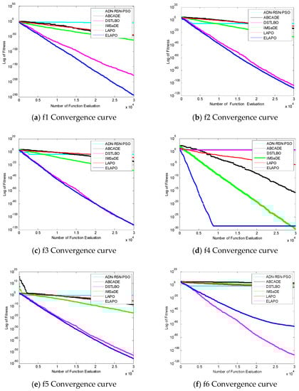
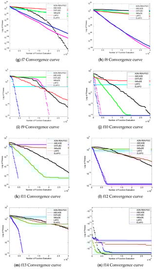
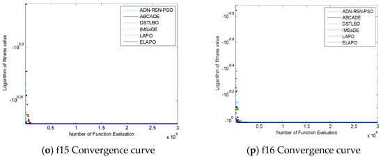
Figure 4. The figure of function convergence.

5. Conclusions and Future Research

In this paper, an improved physical heuristic algorithm ELAPO was proposed. In the downward leader movement by updating the better and the worse particles with a different way and replacing the worst particles in the population with opposition-based learning in the part of enhancement performance, the convergence speed of the algorithm was accelerated. The upward leader jumps out of the local optimum by changing the direction and step size of particle learning. In order to verify the performance of ELAPO, eight single-mode functions and eight multi-mode functions were tested, and the experimental results were compared with those of the better algorithms in recent years. The comparison and analysis of the results showed that the ELAPO algorithm proposed in this paper was superior in solving accuracy and speed, and its performance was stable. The ELAPO algorithm proposed in this paper had certain improvement significance compared with the original algorithm.

In this paper, we only considered the global optimization, and the algorithm could be extended to solve other problems such as constrained optimization problems. In future work, we plan to apply ELAPO to solve real-world domain-specific problems, such as computational offloading problems in mobile edge computing [35].

References

- Boussaid, I.; Lepagnot, J.; Siarry, P. A survey on optimization metaheuristics. Inf. Sci. 2013, 237, 82–117. [Google Scholar] [CrossRef]
- Gogna, A.; Tayal, A. Metaheuristics: Review and application. J. Exp. Theor. Artif. Intell. 2013, 25, 503–526. [Google Scholar] [CrossRef]
- Mahdavi, S.; Shiri, M.E.; Rahnamayan, S. Metaheuristics in large-scale global continues optimization: A survey. Inf. Sci. 2015, 295, 407–428. [Google Scholar] [CrossRef]
- Liu, Y.K.; Li, M.K.; Xie, C.L.; Peng, M.J.; Xie, F. Path-planning research in radioactive environment based on particle swarm algorithm. Prog. Nucl. Energy 2014, 74, 184–192. [Google Scholar] [CrossRef]
- Wari, E.; Zhu, W. A survey on metaheuristics for optimization in food manufacturing industry. Appl. Soft Comput. 2016, 46, 328–343. [Google Scholar] [CrossRef]
- Pyrz, M.; Krzywoblocki, M. Crashworthiness Optimization of Thin-Walled Tubes Using Macro Element Method and Evolutionary Algorithm. Thin Walled Struct. 2017, 112, 12–19. [Google Scholar] [CrossRef]
- Kadin, Y.; Gamba, M.; Faid, M. Identification of the Hydrogen Diffusion Parameters in Bearing Steel by Evolutionary Algorithm. J. Alloys Compd. 2017, 705, 475–485. [Google Scholar] [CrossRef]
- Shieh, M.D.; Li, Y.; Yang, C.C. Comparison of multi-objective evolutionary algorithms in hybrid Kansei engineering system for product form design. Adv. Eng. Inf. 2018, 36, 31–42. [Google Scholar] [CrossRef]
- Yang, J.H.; Honavar, V. Feature Subset Selection Using a Genetic Algorithm. In Feature Extraction, Construction and Selection; Springer: Boston, MA, USA, 1998; pp. 117–136. [Google Scholar]
- Storn, R.; Price, K. Differential Evolution—A Simple and Efficient Heuristic for Global Optimization over Continuous Spaces. J. Glob. Optim. 1997, 11, 341–359. [Google Scholar] [CrossRef]
- Knowles, J.; Corne, D. The Pareto Archived Evolution Strategy: A New Baseline Algorithm for Pareto Multiobjective Optimisation. In Proceedings of the 1999 Congress on Evolutionary Computation-CEC99, Washington, DC, USA, 6–9 July 1999. [Google Scholar]
- Banzhaf, W.; Koza, J.R.; Ryan, C.; Spector, L.; Jacob, C. Genetic programming. IEEE Intell. Syst. 2000, 15, 74–84. [Google Scholar] [CrossRef]
- Hansen, N.; Ostermeier, A. Completely Derandomized Self-Adaptation in Evolution Strategies. Evol. Comput. 2001, 9, 159–195. [Google Scholar] [CrossRef]
- Simon, D. Biogeography-based optimization. IEEE Trans. Evol. Comput. 2008, 12, 702–713. [Google Scholar] [CrossRef]
- Kennedy, J.; Eberhart, R. Particle swarm optimization. In Proceedings of the IEEE International Conference on Neural Networks, Perth, WA, Australia, 27 November–1 December 1995; pp. 1942–1948. [Google Scholar]
- Basturk, B.; Karaboga, D. An artificial bee colony (ABC) algorithm for numeric function optimization. In Proceedings of the IEEE Swarm Intelligence Symposium, Indianapolis, IN, USA, 12–14 May 2006; pp. 687–697. [Google Scholar]
- Mucherino, A.; Seref, O. Monkey search: A novel metaheuristic search for global optimization. AIP Conf. Proc. 2007, 953, 162–173. [Google Scholar]
- Yang, X.S. Firefly Algorithms for Multimodal Optimization. In Proceedings of the 5th International Symposium on Stochastic Algorithms, Foundations and Applications, Sapporo, Japan, 26–28 October 2009; pp. 169–178. [Google Scholar]
- Mirjalili, S.; Mirjalili, S.M.; Lewis, A. Grey Wolf Optimizer. Adv. Eng. Softw. 2014, 69, 46–61. [Google Scholar] [CrossRef]
- Mirjalili, S. Moth-flame optimization algorithm: A novel nature-inspired heuristic paradigm. Knowl. Based Syst. 2015, 89, 228–249. [Google Scholar] [CrossRef]
- Shah-Hosseini, H. Principal components analysis by the galaxy-based search algorithm: A novel metaheuristic for continuous optimisation. Int. J. Comput. Sci. Eng. 2011, 6, 132–140. [Google Scholar]
- Rashedi, E.; Nezamabadi-Pour, H.; Saryazdi, S. GSA: A Gravitational Search Algorithm. Inf. Sci. 2009, 179, 2232–2248. [Google Scholar] [CrossRef]
- Kaveh, A.; Khayatazad, M. A new meta-heuristic method: Ray Optimization. Comput. Struct. 2012, 112, 283–294. [Google Scholar] [CrossRef]
- Hatamlou, A. Black hole: A new heuristic optimization approach for data clustering. Inf. Sci. 2013, 222, 175–184. [Google Scholar] [CrossRef]
- Kaveh, A.; Bakhshpoori, T. Water Evaporation Optimization: A Novel Physically Inspired Optimization Algorithm. Comput. Struct. 2016, 167, 69–85. [Google Scholar] [CrossRef]
- Nematollahi, A.F.; Rahiminejad, A.; Vahidi, B. A Novel Physical Based Meta-Heuristic Optimization Method Known as Lightning Attachment Procedure Optimization. Appl. Soft Comput. 2017, 59, 596–621. [Google Scholar] [CrossRef]
- Wang, H.; Wu, Z.; Liu, Y.; Wang, J.; Jiang, D.; Chen, L. Space transformation search: A new evolutionary technique. In Proceedings of the First ACM/SIGEVO Summit on Genetic and Evolutionary Computation, Shanghai, China, 12–14 June 2009; pp. 537–544. [Google Scholar]
- Suganthan, P.N.; Hansen, N.; Liang, J.J.; Deb, K.; Chen, Y.P.; Auger, A.; Tiwari, S. Problem Definitions and Evaluation Criteria for the CEC 2005 Special Session on Real-Parameter Optimization. Available online: https://www.researchgate.net/profile/Ponnuthurai_Suganthan/publication/235710019_Problem_Definitions_and_Evaluation_Criteria_for_the_CEC_2005_Special_Session_on_Real-Parameter_Optimization/links/0c960525d3990de15c000000/Problem-Definitions-and-Evaluation-Criteria-for-the-CEC-2005-Special-Session-on-Real-Parameter-Optimization.pdf (accessed on 29 June 2019).
- Sun, W.; Lin, A.; Yu, H.; Liang, Q.; Wu, G. All-dimension neighborhood based particle swarm optimization with randomly selected neighbors. Inf. Sci. 2017, 405, 141–156. [Google Scholar] [CrossRef]
- Liang, Z.; Hu, K.; Zhu, Q.; Zhu, Z. An Enhanced Artificial Bee Colony Algorithm with Adaptive Differential Operators. Appl. Soft Comput. 2017, 58, 480–494. [Google Scholar] [CrossRef]
- Bi, X.-J.; Wang, J.-H. Teaching-learning-based optimization algorithm with hybrid learning strategy. J. Zhejiang Univ. Eng. Sci. 2017, 51, 1024–1031. [Google Scholar]
- Wang, S.; Li, Y.; Yang, H.; Liu, H. Self-adaptive differential evolution algorithm with improved mutation strategy. Soft Comput. 2018, 22, 3433–3447. [Google Scholar] [CrossRef]
- Demišar, J.; Schuurmans, D. Statistical Comparisons of Classifiers over Multiple Data Sets. J. Mach. Learn. Res. 2006, 7, 1–30. [Google Scholar]
- Derrac, J.; García, S.; Molina, D.; Herrera, F. A practical tutorial on the use of nonparametric statistical tests as a methodology for comparing evolutionary and swarm intelligence algorithms. Swarm Evol. Comput. 2011, 1, 3–18. [Google Scholar] [CrossRef]
- Guo, F.; Zhang, H.; Ji, H.; Li, X.; Leung, V.C. An Efficient Computation Offloading Management Scheme in the Densely Deployed Small Cell Networks with Mobile Edge Computing. IEEE/ACM Trans. Netw. 2018, 26, 2651–2664. [Google Scholar] [CrossRef]
© 2019 by the authors. Licensee MDPI, Basel, Switzerland. This article is an open access article distributed under the terms and conditions of the Creative Commons Attribution (CC BY) license (http://creativecommons.org/licenses/by/4.0/).