Space-Efficient Fully Dynamic DFS in Undirected Graphs ^†

Abstract

Depth-first search (DFS) is a well-known graph traversal algorithm and can be performed in $O(n+m)$ time for a graph with n vertices and m edges. We consider the dynamic DFS problem, that is, to maintain a DFS tree of an undirected graph G under the condition that edges and vertices are gradually inserted into or deleted from G. We present an algorithm for this problem, which takes worst-case $O(\sqrt{mn}·\mathrm{polylog}\left(n\right))$ time per update and requires only $(3m+o(m\left)\right)\log n$ bits of space. This algorithm reduces the space usage of dynamic DFS algorithm to only 1.5 times as much space as that of the adjacency list of the graph. We also show applications of our dynamic DFS algorithm to dynamic connectivity, biconnectivity, and 2-edge-connectivity problems under vertex insertions and deletions.

1. Introduction

Depth-first search (DFS) is a fundamental algorithm for searching graphs. As a result of performing DFS, a rooted tree (or forest, for disconnected graphs) which spans all vertices is constructed. This rooted tree (forest) is called DFS tree (DFS forest), which is used as a tool for many graph algorithms such as finding strongly connected components of digraphs and detecting articulation vertices or bridges of undirected graphs. Generally, for a graph with n vertices and m edges, DFS can be performed in $O(n+m)$ time, and a DFS tree (forest) can be constructed in the same time.

The graph structure that appears in the real world often changes gradually with time. Therefore, we consider DFS on dynamic graphs, not on static graphs. This problem is called dynamic DFS problem, and the goal for this problem is to design a data structure which can rebuild, for any on-line sequence of updates on G, a DFS tree (forest) for G after each update. Here single update on the graph is one of the following four operations: inserting a new edge, deleting an existing edge, inserting a new vertex and its incident edges (simultaneously), and deleting an existing vertex and its incident edges.

The problem of computing a DFS tree can be classified into two settings. For an undirected graph G, a DFS tree is generally not unique even if a root vertex is fixed. However, if the order of adjacent vertices to visit is fixed for every vertex, the DFS tree will be unique. The ordered DFS tree problem is to compute the order in which the vertices are visited in this setting. Contrary to this, the general DFS tree problem is, given an undirected graph G, to compute any one of DFS trees. In this paper, we focus on the general DFS tree problem. Meanwhile, dynamic graph algorithms can be classified into three types. If an algorithm supports only insertion of edges, it is said to be incremental. If an algorithm supports only deletion of edges, it is called decremental. If an algorithm supports both insertion and deletion updates, it is called fully dynamic. We consider the incremental and fully dynamic settings. Generally, dynamic graph algorithms focus on only edge insertions and deletions. However, for the fully dynamic setting we also consider the vertex insertions and deletions.

1.1. Existing Results

All the works described in this section focus on the general DFS tree problem, not the ordered DFS tree problem. Until recently, there were few papers for the dynamic DFS problem, despite of the simplicity of DFS in static setting. For directed acyclic graphs, Franciosa et al. [1] proposed an incremental algorithm and later Baswana and Choudhary [2] proposed a randomized decremental algorithm. For undirected graphs, Baswana and Khan [3] proposed an incremental algorithm. However, these algorithms support only either of insertion or deletion, and do not support vertex updates. Moreover, none of these algorithms achieve the worst-case time complexity of $o\left(m\right)$ per single update though the amortized update time is better than the static DFS algorithm. This means in the worst case the computational time becomes the same as the static algorithm.

In 2016, Baswana et al. [4] proposed a dynamic DFS algorithm for undirected graphs which overcomes these two problems. Their algorithm supports all four types of graph updates, edge/vertex insertions/deletions, and achieves worst case $O\left(\sqrt{mn}{\log }^{2.5}n\right)$ time per update. They also proposed an incremental (supporting only edge insertions) dynamic DFS algorithm with worst case $O\left(n{\log }^{3}n\right)$ time per update. Later Chen et al. [5] improved the fully dynamic worst-case update time by a $\mathrm{polylog}\left(n\right)$ factor. Baswana et al. also showed in the full version [6] of their paper the conditional lower bounds for fully dynamic DFS problems: $\Omega \left(n\right)$ time per update, under strong exponential time hypothesis, for any fully dynamic DFS under vertex updates, and $\Omega \left(n\right)$ time per update, under the condition the DFS tree is explicitly stored, for any fully dynamic DFS under edge updates. Now the recently proposed incremental dynamic DFS algorithm of Chen et al. [7] has $O\left(n\right)$ worst-case update time and thus meets the lower bound of the incremental setting.

Recently, Baswana et al. [8] conducted an experimental study for the incremental (not fully dynamic) DFS problem. Besides this, Khan [9] proposed a parallel algorithm for the fully dynamic DFS (including vertex updates), which can compute the DFS tree after each update in $O\left({\log }^{3}n\right)$ time using m processors.

Please note that after the preliminary version [10] of this paper was published, Baswana et al. [11] proposed an improved algorithm for the fully dynamic DFS in undirected graphs. This algorithm has worst-case $O\left(\sqrt{mn\log n}\right)$ update time and requires $O\left(m\log n\right)$ bits of space.

1.2. Our Results

We develop algorithms for incremental (i.e., under edge insertions) and fully dynamic (i.e., under edge/vertex insertions/deletions) DFS problems in undirected graphs, based on the algorithms Baswana et al. [4] proposed (an overview of their algorithms is in Section 3). The dynamic DFS algorithms of both Baswana et al. [4] and Chen et al. [5,7] require $O\left(m{\log }^{2}n\right)$ bits of space, which is $O\left(\log n\right)$ times larger than the space usage of the adjacency list of the graph G and thus do not seem to be optimal. Thus, we seek to compress the required space of the dynamic DFS.

Besides this, we focus on relatively dense graphs, i.e., graphs with $n=o\left(m\right)$, because in sparse graphs, i.e., $m=O\left(n\right)$, DFS can be performed in $O\left(n\right)$ time, which meets the conditional lower bound Baswana et al. [6] suggests. Here please note that they showed an example of a graph in which any dynamic DFS algorithm under edge update takes $\Omega \left(n\right)$ time. Since this graph has only $O\left(n\right)$ edges, the (conditional) lower bound holds even for the sparse graphs.

We develop two algorithms for the dynamic DFS algorithm, namely algorithms A and B. Algorithm A is a simple modification of the work of Baswana et al. [4], while algorithm B is designed to reduce the space usage more and more. The comparison of the required space and worst-case update time of these algorithms with those of Baswana et al. [4] and Chen et al. [5,7] is given in Table 1. Both of our algorithms compress the required space by a factor of $O\left(\log n\right)$ and improve the worst-case update time by a $\mathrm{polylog}\left(n\right)$ factor under the fully dynamic case (i.e., supporting all four types of updates). Even under the incremental case (i.e., supporting only edge insertions), the update time is improved from [4], and close to [7]. Our main ingredient is the space usage of algorithm B: it is asymptotically only 1.5 times as much space as that of the adjacency list of G. Here note that since G is undirected, the adjacency list of G should have two elements for each edge in G and thus requires $2m\log n$ bits of space. We also show that if amortized update time is permitted instead of worst-case update time, the required space of algorithm B can be reduced to only $(2m+o(m\left)\right)\log n$ bits.

Table 1. Comparison of required space and worst-case update time for dynamic DFS algorithms.

		Worst-Case Update Time
	Space (bits)	Fully Dynamic	Incremental
[4]	$O\left(m{\log }^{2}n\right)$	$O\left(\sqrt{mn}{\log }^{2.5}n\right)$	$O\left(n{\log }^{3}n\right)$
[5,7]	$O\left(m{\log }^{2}n\right)$	$O\left(\sqrt{mn}{\log }^{1.5}n\right)$	$O\left(n\right)$
A	$O\left(m\log n\right)$	$O\left(\sqrt{mn}{\log }^{0.75+\epsilon }n\right)$	$O{\left(n\sqrt{\log n}\right)}^{*}$
B	$(3m+o(m\left)\right)\log n$	$O\left(\sqrt{mn}{\log }^{1.25}n\right)$	$O\left(n\log n\right)$
[11]	$O\left(m\log n\right)$	$O\left(\sqrt{mn}{\log }^{0.5}n\right)$	−

* If $m=O(n^2/\sqrt{\log n})$, this can be reduced to $O\left(n{\log }^{\epsilon }n\right)$.

Here note that the new dynamic DFS algorithm of Baswana et al. [11] does not subsume algorithm B in terms of the space usage. However, it subsumes algorithm A because the space usage is the same, but the update time is faster. Even so, we describe the details of algorithm A in this paper because, as described below, our algorithm A (as well as algorithm B) can be applied to dynamic biconnectivity and 2-edge-connectivity problems including vertex insertions and deletions.

Our work can be summarized as follows. First, we improve the way to solve a query that is frequently used in the algorithm of Baswana et al. [4] (Section 4), by using the idea of Chen et al. [5] partially. By this improvement, we propose a linear space (i.e., requiring $O\left(m\log n\right)$ bits of space) algorithm, algorithm A, for the incremental and fully dynamic DFS problems (Theorem 1 in Section 5). Second, we further compress the data structures used in [4,5] using wavelet tree [12] (Section 6). In this contribution, we develop an efficient method for solving a kind of query on integer sequences, named range leftmost (rightmost) value query, and give a space-efficient method for solving a variant of orthogonal range search problems, which has been studied in the computational geometry community. These queries are of independent interest. Third, we consider a space-efficient method to implement the algorithm of Baswana et al. [4] (Section 7). By combining them, we propose a more space-efficient algorithm with worst-case update time, algorithm B, for the incremental and fully dynamic DFS problems (Theorems 4 and 5). Simultaneously, results for the amortized update time algorithms are also obtained (Theorems 2 and 3).

1.3. Applications

For static undirected graphs, connectivity, biconnectivity and 2-edge-connectivity queries can be answered by using a DFS tree (details for these queries are in Section 8). The existing fully dynamic DFS algorithms [4,5] can be applied to solve these queries in fully dynamic graphs including vertex updates. Our algorithms can also be extended to answer these queries under the fully dynamic setting including vertex updates. Though we need some additional considerations for our algorithms (Section 8), the worst-case update time complexity and the required space can be kept same as the dynamic DFS algorithms in Table 1 (Theorems 6 and 7). Moreover, as well as the existing fully dynamic DFS algorithms, our algorithms can solve these queries in worst-case $O\left(1\right)$ time.

For the dynamic connectivity problem under vertex updates, the dynamic subgraph connectivity problem [13,14] has been extensively studied. In this problem, given an undirected graph G, a binary status is associated with each vertex in G and we can switch it between “on” and “off”, and the query is to answer whether there is a path between two vertices in the subgraph of G induced by the “on” vertices. Indeed, our dynamic setting including vertex insertions and deletions is a generalization of this dynamic subgraph setting. Under the dynamic subgraph setting, we cannot change the topology of G, i.e., all edges and vertices in G are fixed, while under our setting we can. Under the generalized fully dynamic setting (i.e., our setting), we improve the deterministic worst-case update time bound of [4,5] (with keeping query time $O\left(\mathrm{polylog}\right(n\left)\right)$) by a $\mathrm{polylog}\left(n\right)$ factor. We also compress the required space of their algorithms.

For the dynamic biconnectivity and 2-edge-connectivity problems, the setting including vertex updates was not well considered. Under the fully dynamic setting including vertex updates, we improve the deterministic worst-case update time bound of [4,5] (with keeping query time $O\left(\mathrm{polylog}\right(n\left)\right)$) by a $\mathrm{polylog}\left(n\right)$ factor. We again compress the required space of their algorithms.

2. Preliminaries

Throughout this paper, n denotes the number of vertices and m denotes the number of edges. We assume that a graph is always simple, i.e., has no self-loops or parallel edges, since they make no sense in constructing DFS tree. With this assumption we can conclude $m=O\left(n^2\right)$ and $\log m=O\left(\log n\right)$. We also assume that $n=o\left(m\right)$. We use $\log (·)$ as the base-2 logarithm. From now, the term “fully dynamic setting” includes vertex updates as well as edge updates, while “incremental setting” includes only edge insertions.

Given an undirected graph G and its DFS tree (forest) T, the parent vertex of a vertex v in T is denoted by $par\left(v\right)$. A subtree of T rooted at v is the subgraph of T induced by v and its descendants, and is denoted by $T\left(v\right)$. Two vertices x and y are said to have ancestor-descendant relation iff $x=y$, x is an ancestor of y, or y is an ancestor of x. The path in T connecting two vertices x and y is denoted by $path(x,y)$. A path p in T is called an ancestor-descendant path iff the endpoints of p have ancestor-descendant relation.

Given a connected undirected graph G and its rooted spanning tree T, non-tree edges, i.e., the edges in G which are not included in T, can be classified into two types. A non-tree edge is called a back edge if it connects two vertices which have ancestor-descendant relation; otherwise it is called a cross edge. Then T is a DFS tree of G iff all non-tree edges are back edges. We call this DFS property.

We can assume that the graph G is always connected by the following way. At the beginning, we add a virtual vertex r, and edges $(r,v)$ for all vertices v in G, to the graph G. During our algorithm, we keep a DFS tree of this augmented graph rooted at r. The DFS tree (forest) of the original graph can be obtained by simply removing r from the DFS tree of the augmented graph.

Bit Vectors. Let $B[1\dots l]$ be a 0,1-sequence of length l, and consider two queries on B: for $c=0,1$, ${\mathtt{rank}}_c(i,B)$ returns the number of occurrences of c in $B[1\dots i]$, and ${\mathtt{select}}_c(i,B)$ returns the position of the i-th occurrence of c in B if exists or ∅ otherwise. Then there exists a data structure such that rank and select queries for $c=0,1$ can both be answered in $O\left(1\right)$ time and the required space is $l+O(l\log \log l/\log l)=l+o\left(l\right)$ bits [15,16]. Moreover, the space can be reduced to $l{H}_0\left(B\right)+o\left(l\right)$ bits while keeping $O\left(1\right)$ query time [17], where $H_0\left(B\right)\le 1$ is the zeroth-order empirical entropy of B. When 1 occurs k times in B, $l{H}_0\left(B\right)=k\log \frac{l}{k}+(l-k)\log \frac{l}{l-k}\le k\log \frac{el}{k}$.

Wavelet Trees. Let $S[1\dots l]$ be an integer sequence of symbols $[0,\sigma -1]$. A wavelet tree [12] for S is a complete binary tree with $\sigma$ leaves and $\sigma -1$ internal nodes, each internal node of which has a bit vector [15,16]. Each node v corresponds to an interval of symbols $[l_v,r_v]\subseteq [0,\sigma -1]$; the root corresponds to $[0,\sigma -1]$ and its left (right) child to $[0,\lfloor \sigma /2\rfloor ]$ ($[\lfloor \sigma /2\rfloor +1,\sigma -1]$), and these intervals are recursively divided until leaves, each of which corresponds to one symbol. The bit vector $B_v[1\dots L_v]$ corresponding to an internal node v is defined as follows. Let $S_v[1\dots L_v]$ be the subsequence of S which consists of elements with symbols $[l_v,r_v]$. Then if the symbol $S_v\left[i\right]$ corresponds to the left child of v then $B_v\left[i\right]=0$; otherwise $B_v\left[i\right]=1$. The wavelet tree requires $(l+o(l\left)\right)\log \sigma$ bits of space, and can be built in $O(l\log \sigma /\sqrt{\log l})$ time [18]. Using wavelet tree for S, the following queries can be solved in $O\left(\log \sigma \right)$ time for each: $\mathtt{access}(i,S)$ returns $S\left[i\right]$, ${\mathtt{rank}}_c(i,S)$ returns the number of occurrences of c in $S[1\dots i]$, and ${\mathtt{select}}_c(i,B)$ returns the position of the i-th occurrence of c in B if exists or ∅ otherwise (here $c\in [0,\sigma -1]$).

3. Overview of the Algorithms of Baswana et al.

In this section, we give an overview of the DFS algorithms in dynamic setting proposed by Baswana et al. [4], and describe some lemmas used in this paper.

3.1. Fault Tolerant DFS Algorithm

We first refer to the algorithm for fault tolerant DFS problem. This problem is described as follows: given an undirected graph G and its DFS tree T, we try to rebuild a DFS tree for the new graph obtained by deleting $k(\le n)$ edges and vertices (simultaneously) from G. In this part U denotes a set of vertices and edges we want to delete from G, and $G-U$ denotes the new graph obtained by deleting vertices and edges in U from G.

Their algorithm uses a partitioning technique which divides a DFS tree into connected paths and subtrees. This partitioning is called disjoint tree partitioning (DTP).

Definition 1 ([4]).

A DFS tree T of an undirected graph G and a set U of vertices and edges are given, and the forest $T-U$ obtained by removing the vertices and edges in U from T is considered. Given a vertex subset A of $T-U$, a disjoint tree partitioning of $T-U$ defined by A is a partition of a subgraph of $T-U$ induced by A into a set $\mathcal{P}$ of paths with $\left|\mathcal{P}\right|\le \left|U\right|$ and a set $\mathcal{T}$ of trees. Here each $p\in \mathcal{P}$ is an ancestor-descendant path in T and each $\tau \in \mathcal{T}$ is a subtree of T.

Using DTP, their algorithm can be summarized as follows. First, the DTP of $T-U$ defined by $V\setminus \left\{r\right\}$ (where V is the vertex set of $T-U$ and r is the virtual vertex in Section 2) is calculated. As a result, a set $\mathcal{P}$ of paths and a set $\mathcal{T}$ of subtrees are constructed. Now let $T^{*}$ be the partially constructed DFS tree of $G-U$, and at first $T^{*}$ contains only r. Then their algorithm can be seen as if performing a static DFS traversal (start with r) on the graph whose vertex set is $\mathcal{P}\cup \mathcal{T}$. When a path or a subtree $x\in \mathcal{P}\cup \mathcal{T}$ is visited during the traversal, the algorithm extracts an ancestor-descendant path $p^{*}$ from x and attaches it to $T^{*}$, which means the vertices of $p^{*}$ are marked as visited. Thereafter, the DTP of $T-U$ defined by the unvisited vertices is recalculated. This can be performed by local operations around x. More specifically, if $x\in \mathcal{T}$ the remaining part $x\setminus p^{*}$ is divided into some subtrees and they are stored in $\mathcal{T}$; otherwise $x\setminus p^{*}$ is an ancestor-descendant path and is pushed back to $\mathcal{P}$. Then the traversal continues. If all vertices are visited, $T^{*}$ is indeed the DFS tree of $G-U$.

The key point of reducing computational complexity is that taking advantage of partitioning, the number of edges accessed by this algorithm can be decreased from m. At this time, it must be ensured that the edges not accessed by this algorithm are not needed to construct the new DFS tree $T^{*}$. To achieve this, they use a reduced adjacency list L and two kinds of queries Q and $Q^{\prime }$. Here Q and $Q^{\prime }$ are defined as follows.

Definition 2 ([4]).

A connected undirected graph G, its DFS tree T, and a set U of vertices and edges are given. Then for any three vertices $w,x,y$ in $G-U$, the following queries are considered. Among all edges in $G-U$ which directly connect a subtree $T\left(w\right)$ and an ancestor-descendant path $path(x,y)$, $Q\left(T\right(w),x,y)$ returns one of the edges whose endpoint on $path(x,y)$ is the nearest to x. Similarly, among all edges in $G-U$ which directly connect a vertex w and an ancestor-descendant path $path(x,y)$, $Q^{\prime }(w,x,y)$ returns one of the edges whose endpoint on $path(x,y)$ is the nearest to x. If there are no connecting edges, these queries should return ∅. Here we can assume that $T\left(w\right)$ (or $\left\{w\right\}$) and $path(x,y)$ have no common vertices, and contain no vertices or edges in U.

During the construction of $T^{*}$, the edges added to L are chosen carefully by Q and $Q^{\prime }$ and, instead of the whole adjacency list of G, only L is accessed. Please note that in these queries, the virtual vertex r and its incident edges are not considered, i.e., there are no queries such that $T\left(w\right)$ or $path(x,y)$ contains r.

In fact, this fault tolerant DFS algorithm can be easily extended to handle insertion of vertices/edges as well as deletion updates [4]. Now we consider each of the situations: fully dynamic and incremental. Under the incremental case, the number of times the query Q is called is bounded by $O\left(n\right)$, and $Q^{\prime }$ is not used. In this case, the number of edges in L is at most $O\left(n\right)$. Under the fully dynamic case, the number of times Q and $Q^{\prime }$ is executed is bounded by $O\left(nk\log n\right)$ and $O\left(nk\right)$, respectively, and the number of edges in L is at most $O\left(nk\log n\right)$. Solving these queries Q and $Q^{\prime }$ is the most time-consuming part of their algorithm. Therefore, the time complexity of their fault tolerant DFS algorithm can be summarized in the following lemma.

Lemma 1 ([4]).

An undirected graph G and its DFS tree T are given. Suppose that the query Q can be solved in $O\left(f\right)$ time with a data structure constructed in $O\left(F\right)$ time under the incremental case. Then with $O(F+n)$ preprocessing time, a DFS tree for the graph obtained by applying any $k(\le n)$ edge insertions to G can be built in $O\left(fn\right)$ time. Similarly, suppose Q and $Q^{\prime }$ can be solved in $O\left(g\right)$ and $O\left(g^{\prime }\right)$ time (resp.) with a data structure built in $O\left(G\right)$ time under the fully dynamic case. Then with $O(G+n)$ preprocessing time, a DFS tree for the graph obtained by applying any $k(\le n)$ updates (vertex/edge insertions/deletions) to G can be built in $O\left(k(g\log n+g^{\prime })n\right)$ time.

3.2. Dynamic DFS Algorithm

Next we refer to the algorithm for the dynamic DFS. Baswana et al. [4] proposed an algorithm for this problem by using the fault tolerant DFS algorithm as a subroutine. Their result can be summarized in the following lemma.

Lemma 2 ([4]).

Suppose that for any $k(\le n)$ updates on an undirected graph G, a new DFS tree can be built in $O(kg+h)$ time with a data structure constructed in $O\left(f\right)$ time (i.e., with $O\left(f\right)$ preprocessing time). Then for any on-line sequence of updates on the graph, a new DFS tree after each update can be built in amortized/worst-case $O(\sqrt{fg}+h)$ time per update, if $\sqrt{f/g}\le n$ holds.

First we refer to the amortized (not worst-case) update time algorithm. Their idea is to rebuild the data structure $\mathcal{D}$, which is constructed at the preprocessing in the fault tolerant DFS algorithm, periodically. To explain this idea in detail, let $G_j$ be the graph obtained by applying first $C_j:=c_0+\cdots +c_{j-1}$ updates on G ($c_1,c_2,\dots$ is later decided), $n_j$ and $m_j$ be the number of vertices and edges in $G_j$, and $T_j$ be the DFS tree for $G_j$ reported by this algorithm. For the first $c_0$ updates, use the data structure ${\mathcal{D}}_0$ constructed from the original graph G and DFS tree T. That is, after each arrival of graph update, we perform the fault tolerant DFS algorithm as if all previous updates come simultaneously. After $c_0$ updates are processed, build the data structure ${\mathcal{D}}_1$ from $G_1$ and $T_1$, and use ${\mathcal{D}}_1$ for next $c_2$ updates. In other words, from $(c_0+1)$-st to $(c_0+c_1)$-th updates, we perform the fault tolerant DFS as if from $(c_0+1)$-st to the latest updates come simultaneously. Similarly, after $C_j$ updates are processed, the data structure ${\mathcal{D}}_j$ is built from $G_j$ and $T_j$, and ${\mathcal{D}}_j$ is used for next $c_j$ updates. We call the moment ${\mathcal{D}}_j$ is used phasej of the amortized update time algorithm. In this way the construction time of the data structures is amortized over $c_j$ updates in phase j. Now suppose that for any $k(\le n)$ updates on G, a new DFS tree can be built in $O(k{g}_j+h_j)$ time with ${\mathcal{D}}_j$ built in $O\left(f_j\right)$ time, where $f_j,g_j$ and $h_j$ are all functions of $n_j$ and $m_j$. Then the update time complexity becomes $O(f_j/c_j+g_j{c}_j+h_j)=O(\sqrt{f_j{g}_j}+h_j)$ by setting $c_j=\sqrt{f_j/g_j}$. Therefore, we can achieve the amortized update time bound in Lemma 2. Here in phase j, $f,g$ and h in Lemma 2 are indeed $f_j,g_j$ and $h_j$, and are functions of $n_j$ and $m_j$.

Next we proceed to the worst-case update time algorithm. The idea to achieve the efficient “worst-case” update time described in [4] is to actually divide the construction process of data structure over $c_j$ updates. Here we assume that the number of edges is not dramatically changed during each phase, i.e., $l{m}_j\le m_{j+1}\le h{m}_j$ holds for all $j=1,2,\dots$ with some constants l and h. With this assumption we can say $c_j$ and $c_{j+1}$ differs only by a constant factor (since the number of vertices is not dramatically changed during each phase). In our algorithm described in Section 5 and Section 7, we can say this assumption always holds on condition that $n=o\left(m\right)$, so later we do not touch it.

Let us go into detail. For the first $c_0$ updates, use the data structure ${\mathcal{D}}_0$ built from the original graph G and DFS tree T. For the next $c_1$ updates, use again ${\mathcal{D}}_0$ and build ${\mathcal{D}}_1$ gradually from $G_1$ and $T_1$. Similarly, from $(C_j+1)$-st to $C_{j+1}$-th updates on the graph ($C_j=c_0+\cdots +c_{j-1}$), use ${\mathcal{D}}_{j-1}$ for fault tolerant DFS and build ${\mathcal{D}}_j$ gradually from $G_j$ and $T_j$. In this way the construction time of data structures is divided, and the efficient worst-case update time in Lemma 2 is achieved.

4. Query Reduction to Orthogonal Range Search Problem

In this section, we show an efficient reduction from the queries Q and $Q^{\prime }$ to orthogonal range search queries. Generally speaking, given some points on the grid points, an orthogonal range search problem (in a 2-dimensional plane) is to answer queries about the points within any rectangular region $R=[x_1,x_2]\times [y_1,y_2]$. Queries of this kind are extensively studied in the computational geometry community, e.g., counting the number of points (orthogonal range counting) or reporting all points (orthogonal range reporting) within R. Now we consider the following query.

Definition 3.

On grid points in a 2-dimensional plane, k points are given. Then for any rectangular region $R=[x_1,x_2]\times [y_1,y_2]$, the orthogonal range successor (predecessor) query returns one of the points whose y-coordinate is the smallest (largest) within R. If there are no points within R, the query should return ∅. We abbreviate it as ORS (ORP) query.

4.1. Original Reduction

First we describe the original reduction of queries Q and $Q^{\prime }$ [4] proposed by Baswana et al. In their paper, the ORS (ORP) query is not explicitly used, but is implicitly used. Indeed, their method to answer Q and $Q^{\prime }$ is equivalent to solving $O\left(\log n\right)$ ORS (ORP) queries on the adjacency matrix of G; details are described below. We later use part of their ideas.

Now we describe that how a set of points is constructed from G. The high-level idea is quite simple: the vertices in G are numbered from 0 to $n-1$, and an adjacency matrix according to this numbering is constructed. Let us go into detail. First, a heavy-light (HL) decomposition [19] of T is calculated. Then the order $\mathcal{L}$ of vertices is decided according to the pre-order traversal of T, such that for the first time a vertex v is visited, the next vertex to visit is one that is directly connected with a heavy edge derived from the HL decomposition. Next, the vertices of G (except r) are numbered from 0 to $n-1$ according to $\mathcal{L}$; here the vertex id of v is denoted by $f\left(v\right)$. Finally, on a 2-dimensional grid $\mathcal{G}$, for each edge $(i,j)$ of $G\setminus \left\{r\right\}$, we put two points on the coordinates $\left(f\right(i),f(j\left)\right)$ and $\left(f\right(j),f(i\left)\right)$ in $\mathcal{G}$. This is equivalent to considering the adjacency matrix of G, and thus $2m$ points are placed.

The order $\mathcal{L}$ has some good features. First, for any subtree $T\left(w\right)$ of T, the vertex ids of the vertices of $T\left(w\right)$ occupy single consecutive interval $[t_b,t_e]$ since $\mathcal{L}$ is a pre-order traversal of T. Second, for any ancestor-descendant path $path(x,y)$ in T, those of $path(x,y)$ occupy at most $O\left(\log n\right)$ intervals $[a_1,b_1],\dots ,[a_k,b_k]$. This is because $path(x,y)$ contains at most $O\left(\log n\right)$ light edges (i.e., non-heavy edges) thanks to the property of HL decomposition [19]. Therefore, all edges in G between $T\left(w\right)$ and $path(x,y)$ are within $O\left(\log n\right)$ rectangular regions $[t_b,t_e]\times [a_i,b_i](i=1,\dots ,k)$ on $\mathcal{G}$. Then if $U=\varnothing$ (e.g., the incremental case), the answer for $Q\left(T\right(w),x,y)$ can be obtained by searching them. More specifically, if $f\left(x\right)\le f\left(y\right)$ we solve ORS queries on $\mathcal{G}$ with $R=[t_b,t_e]\times [a_i,b_i](i=1,\dots ,k)$ and return the point with the smallest y-coordinate among the ORS queries’ answers. Otherwise, we solve ORP queries with the same rectangles and return the point with the largest y-coordinate among the ORP queries’ answers. If all ORS (ORP) queries return ∅, the answer for $Q\left(T\right(w),x,y)$ is also ∅. The same argument can be applied for $Q^{\prime }(w,x,y)$ except that the rectangular regions are $[f\left(w\right),f\left(w\right)]\times [a_i,b_i](i=1,\dots ,k)$.

If $U\ne \varnothing$ (e.g., the fully dynamic case), deletion of points on $\mathcal{G}$ should be supported, since the edges in U and the incident edges of the vertices in U must be removed from $\mathcal{G}$ to prevent Q and $Q^{\prime }$ from reporting already deleted edges. To achieve this, Baswana et al. [4] uses a kind of range tree data structures to solve Q and $Q^{\prime }$, which supports deleting a point.

4.2. Efficient Reduction

Next we show the following: (a) the query $Q\left(T\right(w),x,y)$ can be converted to single (not $O\left(\log n\right)$) ORS/ORP query for any $w,x,y$, and (b) the deletion of points from $\mathcal{G}$ need not be supported. Note that the idea to partially achieve (a) is first proposed by Chen et al. [5] and we use a part of it. However, the solution of the query Q of Chen et al. [5] deals with only the case $T\left(w\right)$ is hanging from $path(x,y)$ (that is, the case (ii) in Figure 1 explained later). Thus we here extend this to deal with an arbitrary case. The goal is to prove the following lemma.

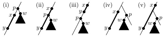
Figure 1. The configurations of $T\left(w\right)$ and $path(x,y)$ in T that can appear in $Q\left(T\right(w),x,y)$.

Lemma 3.

Suppose there exists a data structure $\mathcal{D}$ which can solve both ORS and ORP queries on $\mathcal{G}$ in $O\left(f\right)$ time for each. Then for any three vertices $w,x,y$, the query $Q\left(T\right(w),x,y)$ can be solved in $O\left(f\right)$ time with $\mathcal{D}$. Similarly, for any $w,x,y$ the query $Q^{\prime }(w,x,y)$ can be answered in $O\left(f\log n\right)$ time with $\mathcal{D}$. Please note that $\mathcal{D}$ need not support deletion of points from $\mathcal{G}$.

First we show (a) when $U=\varnothing$ (later this assumption is removed). Here we define some symbols for convenience: for two vertices a and b in G, $a\prec b$ means a is an ancestor of b in T, $a⪯b$ means $a\prec b$ or $a=b$, and $a\parallel b$ means neither $a⪯b$ nor $b⪯a$ holds, i.e., a and b have no ancestor-descendant relation. Let $p=par\left(w\right)$. Please note that it is confirmed that w always has a parent because if w is the root of T, $T\left(w\right)=T$ spans all vertices of G and has some common vertices with any $path(x,y)$, which contradicts the assumption (see Definition 2). Now we assume $x⪯y$ (the case $y\prec x$ is considered at last). Then the configurations of $T\left(w\right)$ and $path(x,y)$ can be classified into five patterns in terms of $x,y$ and p as drawn in Figure 1: (i) $p\prec x⪯y$, (ii) $x⪯p⪯y$, (iii) $x⪯y\prec p$, (iv) $x\parallel p$ and $y\parallel p$, and (v) $x\prec p$ and $y\parallel p$. Now we show the following.

Claim 1.

For all cases from (i) to (v), the answer for $Q\left(T\right(w),x,y)$ can be obtained by solving the ORS query on $\mathcal{G}$ with $R=[t_b,t_e]\times [f\left(x\right),f\left(\mathrm{LCA}(y,w)\right)]$, where $[t_b,t_e]$ is the interval the vertices of $T\left(w\right)$ occupy in the vertex numbering and $\mathrm{LCA}(y,w)$ is the lowest common ancestor of y and w in T.

Proof. 

First, for the cases (i) and (iv), the answer for $Q\left(T\right(w),x,y)$ is ∅ since if such edge exists, it becomes a cross edge and thus refutes DFS property. For these cases, since $\mathrm{LCA}(y,w)$ comes above x and thus $f\left(x\right)>f\left(\mathrm{LCA}\right(y,w\left)\right)$, the ORS query also returns ∅, which correctly answers $Q\left(T\right(w),x,y)$. For other cases ((ii), (iii) and (v)), $\mathrm{LCA}(y,w)$ lies on $path(x,y)$. Here all edges between $T\left(w\right)$ and $path(x,y)$ are indeed between $T\left(w\right)$ and $path(x,\mathrm{LCA}(y,w\left)\right)$ due to DFS property. It may be that the interval $\left[f\right(x),f(\mathrm{LCA}(y,w)\left)\right]$ contains some vertex ids of the vertices of branches forking from $path(x,\mathrm{LCA}(y,w\left)\right)$, which happens when these branches are traversed prior to y and w in $\mathcal{L}$. This does not cause trouble because there are no edges between $T\left(w\right)$ and these branches again due to DFS property. Hence R contains all edges between $T\left(w\right)$ and $path(x,y)$ and no other edges, when we see $\mathcal{G}$ as an adjacency matrix of G. Thus, reporting a point whose y-coordinate is the smallest within R yields an answer for $Q\left(T\right(w),x,y)$. Here note that the LCA query can be solved in $O\left(1\right)$ time with a data structure of $O\left(n\log n\right)=o\left(m\right)\log n$ bits built in $O\left(n\right)$ time [20]. Therefore Claim 1 holds. ☐

From Claim 1 we prove (a) under $U=\varnothing$ and $x⪯y$. Lastly, if $y\prec x$, all we must do is swap x and y and perform almost the same as described above, except that we solve an ORP (not ORS) query on $\mathcal{G}$.

Next we show (b). First we assume that U consists of only vertices and contains no edges. In this setting we can confirm from Definition 2 that for the query $Q\left(T\right(w),x,y)$, $T\left(w\right)$ and $path(x,y)$ have no vertices in U. Thus, $[t_b,t_e]$ contains no vertex ids of the vertices in U. We can also say that even if $\left[f\right(x),f(\mathrm{LCA}(y,w)\left)\right]$ in Claim 1 contains some vertex ids of the vertices in U, these vertices are all in the branches forking from $path(x,y)$ and cause no trouble. Therefore, even if U contains some vertices, Claim 1 also holds. For the query $Q^{\prime }(w,x,y)$, we use the original reduction described in Section 4.1. We can also say from Definition 2 that $\left\{w\right\}$ and $path(x,y)$ have no vertices in U. Thus, $\left[f\right(w),f(w\left)\right]$ and $[a_i,b_i](i=1,\dots ,k)$ contain no vertex ids of the vertices in U.

Finally, we consider the case U contains some edges. In this case, it seems that deletion of these edges from $\mathcal{G}$ is needed. However, deleting one edge $e=(u,v)$ can be simulated by one vertex deletion and one vertex insertion as follows: first record u’s incident edges $(u,w_i)(i=1,2,\dots )$ excluding $e=(u,v)$ itself, second delete v, and then insert a vertex $u^{\prime }$ with its incident edges $(u^{\prime },w_i)(i=1,2,\dots )$. In the algorithm of Baswana et al. [4], vertex insertions are treated separately from the queries Q and $Q^{\prime }$. Thus, in this way we can avoid deleting e from $\mathcal{G}$. This completes the proof of Lemma 3.

Lastly we briefly explain that $Q^{\prime }$ cannot be converted to single ORS (ORP) query in the same way as Q. The five patterns of configuration of vertices drawn in Figure 1 can also appear in $Q^{\prime }(w,x,y)$. However, there is a corner case that can appear in $Q^{\prime }(w,x,y)$ but cannot appear in $Q\left(T\right(w),x,y)$: $w\prec x⪯y$, as drawn in Figure 2. This pattern cannot appear in $Q\left(T\right(w),x,y)$ since if $w\prec x⪯y$ then $T\left(w\right)$ overlaps with $path(x,y)$. This corner case is relatively hard to convert to single ORS/ORP query on $\mathcal{G}$, since every vertex of a branch forking from $path(x,y)$ has ancestor-descendant relation with w. Please note that it does not matter if $Q^{\prime }(w,x,y)$ is solved $O\left(\log n\right)$ times slower than $Q\left(T\right(w),x,y)$ (see Lemma 1).

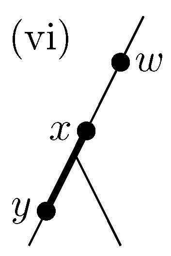
Figure 2. The configuration of $path(x,y)$ and w in T that can appear in $Q^{\prime }(w,x,y)$ and cannot appear in $Q\left(T\right(w),x,y)$.

5. Linear Space Dynamic DFS

In this section, we propose a linear space fast dynamic DFS algorithm. In Section 4.2, we prove that there is no need to support deletion of points from $\mathcal{G}$ even if there are some deletion updates of edges and vertices. This means we can bring a static data structure for the queries Q and $Q^{\prime }$ rather than a dynamic one. Indeed, the data structure by Belazzougui and Puglisi [21] can solve the ORS query in rank space. The rank space with k points is a $[1,k]\times [1,k]$ grid where all points differ in both x- and y-coordinates. For the rank space with k points, their data structure can solve ORS query in $O\left({\log }^{\epsilon }k\right)$ time for an arbitrary $0<\epsilon <1$, can be constructed in $O\left(k\sqrt{\log k}\right)$ time, and occupies $O\left(k\log k\right)$ bits of space. Though $\mathcal{G}$ is not a rank space, we can convert $\mathcal{G}$ to the rank space by using bit vectors. Please note that this kind of conversion is regularly employed for various orthogonal range search data structures (e.g., see [22]). So, in the proof below we do not show the conversion from $\mathcal{G}$ to a rank space, but show that from the adjacency list of G to a rank space directly.

Lemma 4.

There exists a data structure $\mathcal{D}$ which can solve both ORS and ORP queries on $\mathcal{G}$ in $O\left({\log }^{\epsilon }n\right)$ time for each for arbitrary $0<\epsilon <1$. This data structure requires $O\left(m\log n\right)$ bits of space and can be built in $O\left(m\sqrt{\log n}\right)$ time.

Proof. 

Let $d_i$ be the degree of a vertex v in G whose vertex id is i and $M_i={\sum }_{j=0}^{i-1}{d}_j$ ($M_0=0$). Now we have $M_n=2m$, since G is an undirected graph. We construct a rank space $\mathcal{R}$ satisfying the following condition: for two vertices $v,w$ with $f\left(v\right)=i$ and $f\left(w\right)=j$, there exists an edge between v and w in G iff there exists a point within $[M_i+1,M_{i+1}]\times [M_j+1,M_{j+1}]$ in $\mathcal{R}$. This can be done by the following procedure. First, prepare two arrays $A,B$ with $A\left[i\right]=B\left[i\right]=M_i$ for $i=0,\dots ,n-1$. Then for each edge $e=(u,v)$ in G, increment $A\left[f\right(u\left)\right],B\left[f\right(v\left)\right],A\left[f\right(v\left)\right]$ and $B\left[f\right(u\left)\right]$ by one and then place two points on the coordinates $\left(A\right[f\left(u\right)],B[f\left(v\right)\left]\right)$ and $\left(A\right[f\left(v\right)],B[f\left(u\right)\left]\right)$ in $\mathcal{R}$. When all edges are processed, $\mathcal{R}$ satisfies the above condition.

Besides $\mathcal{R}$, we construct a bit vector with $B=0^{d_0}{10}^{d_1}1\cdots 0^{d_{n-1}}1$. Here for $i=0,\dots ,n$, ${\mathtt{rank}}_0({\mathtt{select}}_1(i,B),B)=M_i$ and ${\mathtt{rank}}_1({\mathtt{select}}_0(j,B),B)=i$ for $M_i+1\le j\le M_{i+1}$ $(i\ne n)$. These mean that the bit vector for B enables us to interconvert between the vertex id $f(·)$ and the coordinate in $\mathcal{R}$ in $O\left(1\right)$ time. Therefore, given an ORS query with a rectangle R on $\mathcal{G}$ we can solve it as follows. First, convert the coordinates of R into that in $\mathcal{R}$ by the bit vector for B. Second, solve the converted ORS query on $\mathcal{R}$ by the data structure of Belazzougui and Puglisi [21]. Finally, if the answer is ∅ then the original answer is also ∅. Otherwise the answer is again converted to the vertex id by the bit vector for B. The overall cost for single ORS query is thus $O\left({\log }^{\epsilon }n\right)$. Please note that the bit vector requires only $(n+2m)H_0\left(B\right)+o\left(m\right)\le n\log \frac{e(n+2m)}{n}+o\left(m\right)=o\left(m\right)\log n$ bits of space.

We above mentioned only the ORS query, but the data structure for the ORP query can be built in a similar way. Let ${\mathcal{R}}^{\prime }$ be a rank space constructed by flipping $\mathcal{R}$ vertically; i.e., ${\mathcal{R}}^{\prime }$ is constructed by putting a point on coordinates $(i,2m+1-j)$ for every point $(i,j)$ on $\mathcal{R}$. ${\mathcal{R}}^{\prime }$ can also be built directly from the adjacency list of G, and the ORP query on $\mathcal{G}$ can be converted to the ORS query on ${\mathcal{R}}^{\prime }$ in the same manner as described above. ☐

Figure 3 is an example of an undirected graph G and its corresponding rank space $\mathcal{R}$. In this example, the rectangles $[1,3]\times [4,5]$ and $[4,5]\times [1,3]$ have a point inside, which corresponds to the edge connecting 0 and 1. Conversely, the rectangles $[1,3]\times [6,7]$ and $[6,7]\times [1,3]$ do not have a point inside, which indicates the absence of the edge connecting 0 and 2.

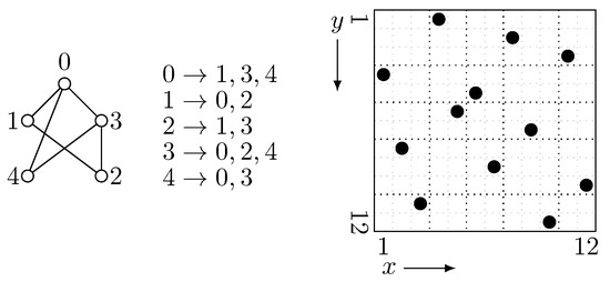
Figure 3. An example of an undirected graph with vertex numbering, its adjacency list, and the corresponding rank space $\mathcal{R}$.

Combining Lemma 4 with Lemma 3 implies the following corollary.

Corollary 1.

There exists a data structure of $O\left(m\log n\right)$ bits such that for any $w,x,y$, $Q\left(T\right(w),x,y)$ can be solved in $O\left({\log }^{\epsilon }n\right)$ time and $Q^{\prime }(w,x,y)$ in $O\left({\log }^{1+\epsilon }n\right)$ time. This data structure can be built in $O\left(m\sqrt{\log n}\right)$ time.

This corollary directly gives a fault tolerant DFS algorithm when combining with Lemma 1. Here we must consider the space requirement of this algorithm, but it is simple. Information used in the algorithm other than the data structure to solve Q and $Q^{\prime }$ and the reduced adjacency list L takes only $O\left(n\log n\right)=o\left(m\right)\log n$ bits: there are $O\left(n\right)$ words of information for the original DFS tree T (including the data representing the disjoint tree partition), $O\left(1\right)$ words of information attached to each vertex and each edge in T, a stack which has at most $O\left(n\right)$ elements, and a partially constructed DFS tree, but these sum up to only $O\left(n\right)$ words. Moreover, since the reduced adjacency list L contains at most $O\left(m\right)$ edges, the required space for L is bounded by $O\left(m\log n\right)$ bits. From Corollary 1, the data structure to solve Q and $Q^{\prime }$ occupies $O\left(m\log n\right)$ bits. Hence the following lemma holds.

Lemma 5.

An undirected graph G and its DFS tree T are given. Then there exists an algorithm such that with $O\left(m\sqrt{\log n}\right)$ preprocessing time, a DFS tree for the graph obtained by applying any $k(\le n)$ edge insertions to G can be built in $O\left(n{\log }^{\epsilon }n\right)$ time. Similarly, there exists an algorithm such that with $O\left(m\sqrt{\log n}\right)$ preprocessing time, a DFS tree for the graph obtained by applying any $k(\le n)$ updates (vertex/edge insertions/deletions) to G can be built in $O\left(nk{\log }^{1+\epsilon }n\right)$ time. These algorithms require $O\left(m\log n\right)$ bits of space.

Linear space dynamic DFS algorithms are obtained by combining Lemma 5 with Lemma 2. For the incremental case, we set $f=m\sqrt{\log n}$, $g=m\sqrt{\log n}/n^2$ and $h=n{\log }^{\epsilon }n$ for Lemma 2 (here the condition $\sqrt{f/g}\le n$ must be satisfied). Then the update time is $O(\sqrt{fg}+h)=O(m/n·\sqrt{\log n}+n{\log }^{\epsilon }n)$. We can say the update time is $O\left(n{\log }^{\epsilon }n\right)$ if $m=O(n^2/\sqrt{\log n})$, or $O\left(n\sqrt{\log n}\right)$ otherwise. For the fully dynamic case, we set $f=m\sqrt{\log n}$, $g=n{\log }^{1+\epsilon }n$ and $h=0$, and, therefore, the update time is $O\left(\sqrt{mn}{\log }^{0.75+\epsilon }n\right)$.

Theorem 1.

There exists an algorithm such that given an undirected graph G and its DFS tree T, for any on-line sequence of updates on G, a new DFS tree after each update can be built in worst-case $O(m/n·\sqrt{\log n}+n{\log }^{\epsilon }n)$ time per update under the incremental case, and $O\left(\sqrt{mn}{\log }^{0.75+\epsilon }n\right)$ time per update under the fully dynamic case, where $0<\epsilon <1/2$ is an arbitrary constant. This algorithm requires $O\left(m\log n\right)$ bits.

6. Compression of Data Structures

In this section, we show a way to solve Q and $Q^{\prime }$ more space-efficiently, which is later used in the space-efficient dynamic DFS algorithm in Section 7.

6.1. Range Next Value Query

First, we show a data structure of $(2m+o(m\left)\right)\log n$ bits, which can be derived immediately from the existing results.

It is already known that the ORS (ORP) query on a $k\times \sigma$ grid ${\mathcal{G}}^{\prime }$ with k points, where all points differ in x-coordinates, can be solved efficiently with wavelet tree [23]. Now we describe this method in detail. The method is to build an integer array $S[1\dots k]$ where $S\left[i\right](1\le i\le k)$ is the y-coordinate of the point whose x-coordinate is i. Then the ORS (ORP) query is converted to the following query on S.

Definition 4.

An integer sequence $S[1\dots l]$ is given. Then for any interval $[a,b]\subseteq [1,l]$ and integer p $\left(q\right)$, the range next (previous) value query returns one of the smallest (largest) elements among the ones in $S[a\dots b]$ which are not less than p (not more than q). If there is no such element, the query should return ∅. We abbreviate it as RN (RP) query.

These queries can be efficiently solved with the wavelet tree $\mathcal{W}$ for S; if $S\left[i\right]\in [0,\sigma -1]$ for all $i=1,\dots ,l$, they can be solved with $O\left(\log \sigma \right)$ rank and select queries on $\mathcal{W}$ [23]. The pseudocode for solving RN query by the wavelet tree for S is given in Algorithm 1. In Algorithm 1, $\mathit{left}\left(v\right)$ and $\mathit{right}\left(v\right)$ stand for the left and right child of the node v, respectively. When calling $\mathrm{RN}(\mathit{root},p,[a,b],[0,\sigma -1\left]\right)$, we can obtain the answer for the RN query with $[a,b]$ and p. Here a pair of the position and the value of the element is returned. If $(0,-1)$ is returned, the answer for the RN query is ∅. The RP queries on S can be solved in a similar way using the same wavelet tree as the RN queries.

Algorithm 1 Range Next Value by Wavelet Tree

1: function RN($v,p,[a,b],[\alpha ,\omega ]$)

2:    if $a>b$ or $\omega <p$ then return $(0,-1)$

3:    if $\alpha =\omega$ then return $(a,\alpha )$

4:    $\gamma \leftarrow ⌊(\alpha +\omega )/2⌋$

5:    if $p\le \gamma$ then

6:        $(pos,val)\leftarrow \mathrm{RN}(\mathit{left}\left(v\right),p,[{\mathtt{rank}}_0(B_v,a-1)+1,{\mathtt{rank}}_0(B_v,b)],[\alpha ,\gamma ])$

7:        if $pos\ne 0$ then return $({\mathtt{select}}_0(B_v,pos),val)$

8:    end if

9:    $(pos,val)\leftarrow \mathrm{RN}(\mathit{right}\left(v\right),p,[{\mathtt{rank}}_1(B_v,a-1)+1,{\mathtt{rank}}_1(B_v,b)],[\gamma +1,\omega ])$

10:    if $pos\ne 0$ then return $({\mathtt{select}}_1(B_v,pos),val)$

11:    else return $(0,-1)$

12: end function

The ORS query on ${\mathcal{G}}^{\prime }$ with $R=[x_1,x_2]\times [y_1,y_2]$ can be answered by solving the RN query on S with $[a,b]=[x_1,x_2]$ and $p=y_1$. If the RN query returns ∅, the answer for the ORS query is also ∅. If the RN query returns an element, the answer is ∅ if the value of this element is larger than $y_2$, or the point corresponding to this element otherwise. Similarly, the ORP query on ${\mathcal{G}}^{\prime }$ can be converted to the RP query on S.

Although in the grid $\mathcal{G}$, on which we want to solve ORS (ORP) queries, some points share the same x-coordinate, it is addressed by preparing a bit vector B in the same way as the proof of Lemma 4. B enables us to convert x-coordinates. Here the integer sequence $S[1\dots 2m]$ consists of the y-coordinates of the points on $\mathcal{G}$ sorted by the corresponding x-coordinates. The required space of the wavelet tree is $(2m+o(m\left)\right)\log n$ bits since there are $k=2m$ points on $\mathcal{G}$ and the y-coordinates vary between $[0,n-1]$. Hence now we obtain a data structure of $(2m+o(m\left)\right)\log n$ bits to solve Q and $Q^{\prime }$ (note that the bit vector requires only $o\left(m\right)\log n$ bits as described in the proof of Lemma 4).

6.2. Halving Required Space

Next, we propose a data structure of $(m+o(m\left)\right)\log n$ bits to solve Q and $Q^{\prime }$. The data structure shown in Section 6.1 has information of both directions for each edge of G since G is an undirected graph. This seems to be redundant, thus we want to hold information of only one direction for each edge. In fact, the placement of points on $\mathcal{G}$ is symmetric since the adjacency matrix of G is also symmetric. So now we consider, of the grid $\mathcal{G}$, the upper triangular part ${\mathcal{G}}_u$ and the lower triangular part ${\mathcal{G}}_l$; a grid ${\mathcal{G}}_u$ inherits from $\mathcal{G}$ the points within the region the x-coordinate is larger than the y-coordinate, and ${\mathcal{G}}_l$ is defined in the same manner. Since G has no self-loops, ${\mathcal{G}}_u$ and ${\mathcal{G}}_l$ have m points for each. Now we show that we can use ${\mathcal{G}}_u$ as a substitute for $\mathcal{G}$.

Let $S_u[1\dots m]$ be an integer sequence which contains the y-coordinates of the points on ${\mathcal{G}}_u$ sorted by the corresponding x-coordinates. Let $B_u$ be a bit vector $0^{d_{0,u}}{10}^{d_{1,u}}1\cdots 0^{d_{n-1,u}}1$, where $d_{i,u}$ is the number of occurrences of i in $S_u$. $B_u$ enables us to convert the x-coordinate on $\mathcal{G}$ to the position in $S_u$ and vice versa in $O\left(1\right)$ time. Figure 4 is an example of the grid $\mathcal{G}$ and its upper triangular part ${\mathcal{G}}_u$. Here we should observe that ${\mathcal{G}}_u$ has half as much point as $\mathcal{G}$ and thus the length of $S_u$ is halved from S.

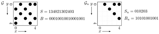
Figure 4. (Left) an example of the grid $\mathcal{G}$ and its corresponding array S and bit vector B. Please note that this grid corresponds to the graph in Figure 3. (Right) the upper triangular part ${\mathcal{G}}_u$ and its corresponding array $S_u$ and bit vector $B_u$.

Lemma 6.

Any ORS (ORP) query which appears in the reduction of Lemma 3 can be answered by solving one RN (RP) query, or by solving onerankand oneselectqueries, on $S_u$.

Proof. 

We give a proof for only ORS queries since that for ORP queries is almost same. It can be observed that if the query rectangle of the ORS query is inside the upper triangular part of $\mathcal{G}$, this ORS query can be converted to an RN query on $S_u$ in the same way as Section 6.1, since ${\mathcal{G}}_u$ contains all points inside the upper triangular part in $\mathcal{G}$. The below claim ensures us that any ORS query related to Q can be converted to the RN query on $S_u$.

Claim 2.

The rectangles appearing in Claim 1 are all inside the upper triangular part of $\mathcal{G}$, i.e., these rectangles are of the form: $[x_1,x_2]\times [y_1,y_2]$ with $y_1\le y_2<x_1\le x_2$.

Proof. 

It can be easily observed that $t_b$, appearing in the interval $[t_b,t_e]$ corresponding to the vertices of a subtree $T\left(w\right)$, equals to $f\left(w\right)$. Since $\mathrm{LCA}(y,w)⪯p\prec w$, $f\left(\mathrm{LCA}\right(y,w\left)\right)\le f\left(p\right)<f\left(w\right)$ and thus $[t_b,t_e]\times [f\left(x\right),f\left(\mathrm{LCA}(y,w)\right)]$ is inside the upper triangular part. ☐

In solving $Q^{\prime }$, there may be query rectangles inside the lower triangular part. However, these rectangles are of the form: $\left[f\right(w),f(w\left)\right]\times [a,b]$ with $f\left(w\right)<a\le b$. Transposing this rectangle, it is inside the upper triangular part and the problem becomes like the following: for a rectangle $R=[a,b]\times [c,c]$ (with $c<a\le b$) on ${\mathcal{G}}_u$, we want to know the point whose “x-coordinate” is the smallest within R. Converting the x-coordinate to the position in $S_u$ by $B_u$, this problem is equivalent to the following problem: to find the leftmost element among ones in $S_u[a^{\prime }\dots b^{\prime }]$ with a value just c.

Claim 3.

Finding the leftmost element among ones in $S_u[a^{\prime }\dots b^{\prime }]$ with a value just c can be done by onerankand oneselectqueries on $S_u$ for any $a^{\prime },b^{\prime },c$.

Proof. 

Let $k={\mathtt{rank}}_c(a^{\prime }-1,S_u)$. It is observed that the $(k+1)$-st occurrence of c in $S_u$ is the answer if it exists and its position is in $[a^{\prime },b^{\prime }]$. So, if ${\mathtt{select}}_c(k+1,S_u)$ returns ∅ or a value more than $b^{\prime }$ then the answer is “not exist”. Otherwise the answer can be obtained by this select query itself. ☐

This completes the proof of Lemma 6. ☐

Since rank, select, RN and RP queries on $S_u$ can be solved in $O\left(\log n\right)$ time for each with a wavelet tree for $S_u$, we immediately obtain a data structure of $(m+o(m\left)\right)\log n$ bits for the queries Q and $Q^{\prime }$. Here the required space of $B_u$ is again $o\left(m\right)\log n$ bits and does not matter.

Corollary 2.

There exists a data structure of $(m+o(m\left)\right)\log n$ bits such that for any $w,x,y$, $Q\left(T\right(w),x,y)$ can be solved in $O\left(\log n\right)$ time and $Q^{\prime }(w,x,y)$ in $O\left({\log }^{2}n\right)$ time. This data structure can be built in $O\left(m\sqrt{\log n}\right)$ time.

Please note that the above corollary does not mention working space for the construction of the data structure. Therefore, obtaining space-efficient dynamic DFS algorithm requires consideration of the building process, since in the algorithm of Baswana et al. we need to rebuild this data structure periodically. We further consider this in Section 7.

6.3. Range Leftmost Value Query

Next, we show another way to compress the data structure to $(m+o(m\left)\right)\log n$ bits. This is achieved by solving range leftmost (rightmost) value query with a wavelet tree. This query appears in the preliminary version [10] of this paper. In the preliminary version, this query and the RN (RP) query (Definition 4) is used simultaneously to obtain a data structure of $(m+o(m\left)\right)\log n$ bits. Although we no longer need to use this query to halve the required space as described in Section 6.2, this query still gives us another way to compress the data structure. Moreover, this query is of independent interest since its application is beyond the dynamic DFS algorithm, as described later.

The range leftmost (rightmost) value query is defined as follows.

Definition 5.

An integer sequence $S[1\dots l]$ is given. Then for any interval $[a,b]\subseteq [1,l]$ and two integers $p\le q$, the range leftmost (rightmost) value query returns the leftmost (rightmost) element among the ones in $S[a\dots b]$ with a value not less than p and not more than q. If there is no such element, the query should return ∅. We abbreviate it as RL (RR) query.

This RL (RR) query is a generalization of the query of Claim 3 in the sense that the value of elements we focus varies between $[p,q]$ instead of being fixed to just c. Moreover, the RL (RR) query is a generalization of a prevLess query [24], which is the RR query with $a=1$ and $p=0$. It is already known that the prevLess query can be efficiently solved with the wavelet tree for S [24].

First we describe the idea to use RL (RR) query for solving Q and $Q^{\prime }$. Here we consider the symmetric variant of ORS (ORP) query, which is almost the same as ORS (ORP) query except that it returns one of the points whose “x-coordinate” is the smallest (largest) within R (we call it symmetric ORS (ORP) query). The motivation to consider symmetric ORS (ORP) queries comes from transposing the query rectangle of normal ORS (ORP) queries. Since $\mathcal{G}$ is symmetric, the (normal) ORS query on $\mathcal{G}$ with rectangle $R=[x_1,x_2]\times [y_1,y_2]$ is equivalent to the symmetric ORS query on $\mathcal{G}$ with rectangle $R^{\top }=[y_1,y_2]\times [x_1,x_2]$. When transposing the rectangle, we can focus on the lower triangular part ${\mathcal{G}}_l$ instead of the upper triangular part ${\mathcal{G}}_u$, as described below.

Let $S_l$ and $B_l$ be an integer sequence and a bit vector constructed from ${\mathcal{G}}_l$ in the same manner as $S_u$ and $B_u$. $B_l$ enables us to convert between the x-coordinate on ${\mathcal{G}}_l$ and the position in $S_u$. Then it can be observed that the symmetric ORS query on ${\mathcal{G}}_l$ with $R=[x_1,x_2]\times [y_1,y_2]$ can be answered by solving the RL query on $S_l$ with $[a,b]=[x_1^{\prime },x_2^{\prime }]$ and $[p,q]=[y_1,y_2]$, where $[x_1^{\prime },x_2^{\prime }]$ is the interval of the position in $S_l$ corresponding to $[x_1,x_2]$. If the RL query returns ∅, the answer for the symmetric ORS query is also ∅. Otherwise the answer can be obtained by converting the returned position in $S_l$ to the x-coordinate on ${\mathcal{G}}_l$ by $B_l$. In this reduction “leftmost” means “the smallest x-coordinate”. Similarly, a symmetric ORP query on ${\mathcal{G}}_l$ can be converted to an RR query on $S_l$. With this conversion from the symmetric ORS (ORP) query to the RL (RR) query, we can prove the following lemma which is a lower triangular version of Lemma 6.

Lemma 7.

Any ORS (ORP) query which appears in the reduction of Lemma 3 can be answered by solving one RL (RR) query, or by solving onerankand oneselectqueries, on $S_l$.

Proof. 

From Claim 2, the rectangles of the ORS queries corresponding to Q is all inside the upper triangular part. Therefore, when we transpose them, they are inside the lower triangular part. Since the symmetric ORS query can be converted into the RL query as described above, it is enough for solving Q. In solving $Q^{\prime }$, there may be query rectangles inside the upper triangular part. However, they are solved by one rank and one select queries on $S_l$, in the same way as Claim 3. ☐

Next we describe how to solve RL (RR) queries with a wavelet tree. We prove the following lemma, by referring to the method to solve prevLess [24] by a wavelet tree.

Lemma 8.

An integer sequence $S[1\dots l]$ is given. Suppose that $S\left[i\right]\in [0,\sigma -1]$ for all $i=1,\dots ,l$. Then using the wavelet tree for S, both RL and RR queries can be answered in $O\left(\log \sigma \right)$ time for each.

Proof. 

We show that with the pseudocode given in Algorithm 2. First we show the correctness. In the arguments of $\mathrm{RL}$, v is the node of the wavelet tree we are present, and $[\alpha ,\omega ]$ is the interval of symbols v corresponds to (i.e., $[\alpha ,\omega ]=[l_v,r_v]$). We claim the following, which ensures us that the answer for the RL query can be obtained by calling $\mathrm{RL}(\mathit{root},[p,q],[a,b],[0,\sigma -1\left]\right)$. ☐

Claim 4.

For any node v of wavelet tree and four integers $a,b,p,q$, calling $\mathrm{RL}(v,[p,q],[a,b],[l_v,r_v])$ yields the position of the answer for the RL query on $S_v$. If the answer for the RL query is ∅, this function returns 0.

Proof. 

We use an induction on the depth of the node v. The base case is $[l_v,r_v]\cup [p,q]=\varnothing$ or $[l_v,r_v]\subseteq [p,q]$ (note that either of them must occur when $l_v=r_v$, so if v is a leaf node the basis case must happen). For the former case, the answer is obviously ∅. For the latter case, the answer is a since all elements in $S_v[a\dots b]$ have value between $[l_v,r_v]\subseteq [p,q]$. In these cases, the answer is correctly returned with lines 2–3 of Algorithm 2.

Now we proceed to the general case. Let $l\left(v\right)=\mathit{left}\left(v\right)$, $r\left(v\right)=\mathit{right}\left(v\right)$ and $\gamma =\lfloor (l_v+r_v)/2\rfloor$. Then $[l_{l\left(v\right)},r_{l\left(v\right)}]=[l_v,\gamma ]$ and $[l_{r\left(v\right)},r_{r\left(v\right)}]=[\gamma +1,r_v]$. Therefore, the elements in $S_v[a\dots b]$ with a value between $[l_v,\gamma ]$ appear in the left child $S_{l\left(v\right)}[a_l\dots b_l]$, and those with a value between $[\gamma +1,r_v]$ appear in the right child $S_{r\left(v\right)}[a_r\dots b_r]$. Here $a_l,b_l,a_r$ and $b_r$ can be calculated by rank queries on $B_v$: $[a_l,b_l]=[{\mathtt{rank}}_0(B_v,a-1)+1,{\mathtt{rank}}_0(B_v,b)]$ and $[a_r,b_r]=[{\mathtt{rank}}_1(B_v,a-1)+1,{\mathtt{rank}}_1(B_v,b)]$. It can be observed that the element $S_v\left[i^{\prime }\right]$ of $S_v$ corresponding to the leftmost element $S_{l\left(v\right)}\left[i\right]$ in $S_{l\left(v\right)}[a_l,b_l]$ with a value within $[p,q]$ is also the leftmost element in $S_v[a\dots b]$ with a value within $[p,q]\cap [l_v,\gamma ]$. Here i can be obtained by $\mathrm{RL}(l\left(v\right),[p,q],[a_l,b_l],[l_v,\gamma ])$ (induction hypothesis) and $i^{\prime }={\mathtt{select}}_0(B_v,i)$. Similarly, the element $S_v\left[j^{\prime }\right]$ of $S_v$ corresponding to the leftmost element $S_{r\left(v\right)}\left[i\right]$ in $S_{r\left(v\right)}[a_r,b_r]$ with a value within $[p,q]$ is also the leftmost element in $S_v[a\dots b]$ with a value within $[p,q]\cap [\gamma +1,r_v]$. Again j can be obtained by $\mathrm{RL}(r\left(v\right),[p,q],[a_r,b_r],[\gamma +1,r_v])$ (induction hypothesis) and $j^{\prime }={\mathtt{select}}_1(B_v,j)$. Hence $S_v[min\{i^{\prime },j^{\prime }\}]$ is the leftmost element we want to know. Now the answer is correctly returned with lines 4–10 of Algorithm 2: lines 7–10 cope with the case the $\mathrm{RL}$ function returns 0. ☐

Next we discuss the time complexity when calling $\mathrm{RL}(v,[p,q],[a,b],[l_v,r_v])$. We show that for each level (depth) of the wavelet tree the function visits at most four nodes. At the top level we visit only one node $\mathit{root}$. At level k, the general case occurs at most two times: it may occur when $[l_v,r_v]$ contains the endpoints of $[p,q]$. Thus, at level $k+1$ the $\mathrm{RL}$ function is called at most $2\times 2=4$ times. Since the wavelet tree has depth $\lceil \log \sigma \rceil$, $\mathrm{RL}$ function is called $O\left(\log \sigma \right)$ times. For each node, all calculation other than the recursion can be done in $O\left(1\right)$ time, so the overall time complexity is $O\left(\log \sigma \right)$.

The same argument can be applied for the RR query. This completes the proof. ☐

Algorithm 2 Range Leftmost Value by Wavelet Tree

1:function RL($v,[p,q],[a,b],[\alpha ,\omega ]$)

2:    if $a>b$ or $[\alpha ,\omega ]\cap [p,q]=\varnothing$ then return 0

3:    if $[\alpha ,\omega ]\subseteq [p,q]$ then return a

4:    $\gamma \leftarrow ⌊(\alpha +\omega )/2⌋$

5:    $i\leftarrow \mathrm{RL}(\mathit{left}\left(v\right),[p,q],[{\mathtt{rank}}_0(B_v,a-1)+1,{\mathtt{rank}}_0(B_v,b)],[\alpha ,\gamma ])$

6:    $j\leftarrow \mathrm{RL}(\mathit{right}\left(v\right),[p,q],[{\mathtt{rank}}_1(B_v,a-1)+1,{\mathtt{rank}}_1(B_v,b)],[\gamma +1,\omega ])$

7:    if $i\ne 0$ and $j\ne 0$ then return $min({\mathtt{select}}_0(B_v,i),{\mathtt{select}}_1(B_v,j))$

8:    else if $i\ne 0$ then return ${\mathtt{select}}_0(B_v,i)$

9:    else if $j\ne 0$ then return ${\mathtt{select}}_1(B_v,j)$

10:    else return 0

11: end function

Lemmas 7 and 8 imply another way to achieve Corollary 2.

Finally, we discuss the application of RL (RR) query beyond the dynamic DFS algorithm. Let us consider ORS and ORP queries on an $l\times l$ grid $\mathcal{S}$ whose placement of points is symmetric. Suppose that there are d points on a diagonal line of $\mathcal{S}$ (we call them diagonal points) and $2k$ points within the other part of $\mathcal{S}$. Generally, there is no assumption on query rectangles such as Claim 2, so with only RN (RP) queries we cannot remove the points within the lower triangular part of $\mathcal{S}$. However, using RL (RR) queries as well as RN (RP) queries, we can consider only the upper triangular and the diagonal parts of $\mathcal{S}$. The idea, which is very similar to the method in the preliminary version [10] of this paper, is as follows. First, for a query rectangle $R=[x_1,x_2]\times [y_1,y_2]$ of the ORS (ORP) query, we solve the corresponding RN (RP) query. Second, for the transposed query rectangle $R^{\top }=[y_1,y_2]\times [x_1,x_2]$, we solve the corresponding RL (RR) query, and “transpose” the answer. Finally, we combine these two answers: choose the one with smaller (larger) y-coordinate. Let $S_{ud}$ and $B_{ud}$ be an integer sequence and a bit vector constructed from the upper triangular and the diagonal parts of $\mathcal{S}$ in the same manner as $S_u$ and $B_u$. A wavelet tree for $S_{ud}$ can solve RN, RP, RL and RR queries on $S_{ud}$ and occupies $(k+d+o(k)+o(d\left)\right)\log l$ bits, since the diagonal part has d points and the upper triangular part has k points. Because the space required for $B_{ud}$ is not a matter, now we obtain a space-efficient data structure for solving ORS and ORP queries on $\mathcal{S}$. If $d=0$, the required space of the data structure is actually halved from using wavelet tree directly ($(2k+d+o(k)+o(d\left)\right)\log n$ bits).

If d is large, we can further compress the space from $(k+d+o(k)+o(d\left)\right)\log l$ bits by treating diagonal points separately. Let $B_d[1\dots l]$ be a bit vector such that $B_d\left[i\right]=1$ if there exists a point on coordinates $(i,i)$ and $B_d\left[i\right]=0$ otherwise. For a query rectangle $R=[x_1,y_1]\times [x_2,y_2]$, let $[a,b]=[max\{x_1,y_1\},min\{x_2,y_2\}]$. Then it can be easily observed that R contains diagonal lines from $(a,a)$ to $(b,b)$ if $a\le b$ and R has no diagonal points otherwise. Therefore if $a\le b$, a diagonal point with smallest (largest) y-coordinate within R can be obtained by one rank and one select query on $B_d$. Now we do not retain the information of the diagonal points in the wavelet tree, so the overall required space of data structures is $(k+o\left(k\right))\log l+l{H}_0\left(B_d\right)+o\left(l\right)\le (k+o\left(k\right))\log l+d\log \frac{el}{d}+o\left(l\right)$ bits.

7. More Space-Efficient Dynamic DFS

In this section, we show algorithms to solve the dynamic DFS problem space-efficiently. Our algorithm is based on the algorithms of Baswana et al. [4], but there is much consideration in compressing the working space of it.

7.1. Fault Tolerant DFS

We begin with the algorithm for the fault tolerant DFS problem. Following the original algorithm described in Section 3.1, the important point is that once a data structure for answering Q and $Q^{\prime }$ is built, the reduced adjacency list L is used and the whole adjacency list of the original graph is no longer needed. Moreover, information used in the algorithm other than the data structure and the reduced adjacency list takes only $O\left(n\log n\right)=o\left(m\right)\log n$ bits, as described in Section 5. Since we have already shown in Corollary 2 that the data structure takes $(m+o(m\left)\right)\log n$ bits, we have only to consider the size of the reduced adjacency list L. From Section 3.1, for any $k(\le n)$ graph updates, the number of edges in L is at most $O\left(n\right)$ under the incremental case, and $O\left(nk\log n\right)$ under the fully dynamic case. The time complexity of this algorithm can be calculated from Lemma 1 and Corollary 2. The required space of this algorithm is $(m+o(m\left)\right)\log n$ bits plus the space required for L, that is, $O\left(m_L\log n\right)$ bits (with standard linked lists) where $m_L$ is the upper bound of the number of edges in L. To sum up, we can obtain the following lemma.

Lemma 9.

An undirected graph G and its DFS tree T are given. Then there exists an algorithm such that with $O\left(m\sqrt{\log n}\right)$ preprocessing time, a DFS tree for the graph obtained by applying any $k(\le n)$ edge insertions to G can be built in $O\left(n\log n\right)$ time. This algorithm requires $(m+o(m\left)\right)\log n$ bits once the preprocessing is finished. Similarly, there exists an algorithm such that with $O\left(m\sqrt{\log n}\right)$ preprocessing time, a DFS tree for the graph obtained by applying any $k(\le n)$ updates (vertex/edge insertions/deletions) to G can be built in $O\left(nk{\log }^{2}n\right)$ time. This algorithm requires $(m+o\left(m\right))\log n+O\left(nk{\log }^{2}n\right)$ bits once the preprocessing is finished.

7.2. Amortized Update Time Dynamic DFS

Next, we focus on the amortized update time dynamic DFS algorithm. During the “amortized time” algorithm described in Section 3.2, we should perform the reconstruction of the data structure $\mathcal{D}$ to solve the fault tolerant DFS problem besides the fault tolerant DFS itself, and store information of up to last c updates. Here $\mathcal{D}$ is indeed a bit vector and a wavelet tree described in Section 6. Therefore, we must consider (a) how many edges the reduced adjacency list L may have, (b) how much space is required to store information of updates, and (c) how to rebuild the data structure space-efficiently. We analyze these issues one by one.

First we consider (a). Since we rebuild $\mathcal{D}$ periodically, we solve the fault tolerant DFS problem with at most $c_j$ updates in phase j. Therefore, we can obtain an upper bound on the number of edges in L. Under the incremental case, we can say $f=m\sqrt{\log n},g=\sqrt{\log n}$ and $h=n\log n$ for Lemma 2 (here $\sqrt{f/g}=\sqrt{m}\le n$ holds), and the size of L is bounded by $O\left(n\right)$, as described in Section 7.1. Under the fully dynamic case, we can say $f=m\sqrt{\log n},g=n{\log }^{2}n$ and $h=0$, thus the upper bound is $O(n\log n·\sqrt{f/g})=O\left(\sqrt{mn}{\log }^{0.25}n\right)$ which is $o\left(m\right)$ under the assumption $m=\omega \left(n{\log }^{0.5}n\right)$. Hence we can conclude that L takes only $o\left(m\right)\log n$ bits under any conditions.

Next we consider (b), but this is almost the same as (a). Under the incremental case, the number of edges inserted during $c_j$ updates is up to $\sqrt{f/g}=\sqrt{m}$ which is $o\left(m\right)$. Under the fully dynamic case, the number of edges inserted or deleted during $c_j$ updates is up to $O\left(n\sqrt{f/g}\right)=O(\sqrt{mn}/{\log }^{0.75}n)$, since insertion or deletion of one vertex involves those of $O\left(n\right)$ incident edges. This is smaller than the maximum size of L, and thus it does not affect the bound. Please note that in the analysis of (a) and (b), we write $n_j,m_j,f_j,g_j,h_j$ in Section 3.2 as $n,m,f,g,h$ for simplicity.

Finally, we consider (c). Let ${\mathcal{L}}_j$ be the order of vertices in $G_j$ defined by the pre-order traversal of $T_j$, where $G_j$ and $T_j$ are the graph and its reported DFS tree at the beginning of phase j of the amortized update time algorithm, and let ${\mathcal{G}}_j$ be the grid like $\mathcal{G}$ constructed from $G_j$ and ${\mathcal{L}}_j$ (in our algorithm we do not retain ${\mathcal{G}}_j$, but it helps the description of our algorithm clear). In addition to these, let $S_j[1\dots m_j]$ and $B_j$ be an integer sequence and a bit vector built from the upper (or lower) triangular part of ${\mathcal{G}}_j$ in the same manner as Section 6 (in Section 6, they are written as $S_u$ and $B_u$ (or $S_l$ and $B_l$)). Now we focus on the end of phase j, i.e., the time $T_{j+1}$ is reported. Using these symbols, the rebuilding process at this moment is briefly described as follows. First, the order of vertices ${\mathcal{L}}_{j+1}$ is decided according to the pre-order traversal of $T_{j+1}$, and information attached to each vertex and edge of $T_{j+1}$ is initialized. Second, a grid ${\mathcal{G}}_{j+1}$ is considered, and $S_{j+1}$ and $B_{j+1}$ are built. Finally, a wavelet tree ${\mathcal{W}}_{j+1}$ for $S_{j+1}$ is constructed.

The main difficulty in this rebuilding process is that the whole adjacency list is not retained. That means the information of all edges in $G_{j+1}$ is not explicitly stored at this moment. It is stored in the wavelet tree ${\mathcal{W}}_j$ for $S_j$, the bit vector $B_j$, and the information of the last $c_j$ updates. In our algorithm, we additionally retain the integer sequence $S_j$ during phase j of the algorithm. Then the main job in this moment is to construct $S_{j+1}$ and $B_{j+1}$ from $S_j$, $B_j$ and the information of last $c_j$ updates.

To do this, we also retain during phase j an integer sequence $M_j[0\dots n_j]$, where $M_j\left[i\right]$ is the number of points in the upper (or lower) triangular part of ${\mathcal{G}}_j$ whose x-coordinate is less than i. Then $0=M_j\left[0\right]\le M_j\left[1\right]\le \cdots \le M_j\left[n_j\right]=m_j$ holds. The y-coordinates of the points whose x-coordinate is i are stored in $S_j[M_j\left[i\right]+1\dots M_j[i+1]]$; we call this subsequence a block i of $S_j$. We impose a condition on $S_j$ that each block of $S_j$ is sorted in ascending order. Please note that $S_j$ takes $m_j\log n_j$ bits and $M_j$ takes $O\left(n_j\log m_j\right)=o\left(m_j\right)\log n_j$ bits.

Now we describe the way to rebuild the data structures space-efficiently at the end of phase j. First, destroy $B_j$ and ${\mathcal{W}}_j$. Second, sort the information of last $c_j$ updates, i.e., the inserted or deleted edges during the last c updates, in the same order as $S_j$. This can be performed as follows. First convert this information to tuples $(x_i,y_i,d_i)$ where $(x_i,y_i)$ is the vertex ids (according to ${\mathcal{L}}_j$) of the endpoints of the edge with $x_i>y_i$ (or $x_i<y_i$ in the lower triangular case), and $d_i$ is information of 1 bit which represents whether the edge is inserted or deleted (here if there are inserted vertices, they are numbered from $n_j$). Second sort them by the ascending order of $x_i$. If there are some tuples which share $x_i$, they are sorted by the ascending order of $y_i$. Please note that since the number of edges inserted or deleted during $c_j$ updates is up to $o\left(m_j\right)$, sorting can be performed in linear time (i.e., $o\left(m_j\right)$ time) and $o\left(m_j\right)\log n_j$ bits of working space by radix sort. Third, create a new array $S_{j+1}^{\prime }[1\dots m_{j+1}]$ and $M_{j+1}^{\prime }[0\dots n_{j+1}]$, which retains information of all edges in $G_{j+1}$ with the vertex numbering from ${\mathcal{L}}_j$. This can be done by simply scanning the tuples and $S_j$ simultaneously and merging them, since they are sorted in the same order. Fourth, destroy $S_j$ and $M_j$, and decide the order ${\mathcal{L}}_{j+1}$ of vertices in $G_{j+1}$ according to the pre-order traversal of $T_{j+1}$. Fifth, create $S_{j+1}[1\dots m_{j+1}]$ and $M_{j+1}[0\dots n_{j+1}]$ from $S_{j+1}^{\prime }$ and $M_{j+1}^{\prime }$, and destroy $S_{j+1}^{\prime }$ and $M_{j+1}^{\prime }$. The detail of this process is described later. Finally, build ${\mathcal{W}}_{j+1}$ and $B_{j+1}$ from $M_{j+1}$ and $S_{j+1}$. Then we are ready for phase $(j+1)$.

The remaining part is creating $S_{j+1}$ and $M_{j+1}$ from $S_{j+1}^{\prime }$ and $M_{j+1}^{\prime }$. For simplicity, let $t=j+1$, and suppose that we now focus on the upper triangular part of ${\mathcal{G}}_t$ as in Section 6.2 (even if we focus on the lower triangular part of ${\mathcal{G}}_t$ as in Section 6.3, we can perform this in almost the same way). First, construct an old-to-new correspondence table N of vertex numbering: $N\left[i\right]$ is the vertex id from ${\mathcal{L}}_t$ of a vertex whose vertex id from ${\mathcal{L}}_j$ is i. Then the pseudocode for converting $S_t^{\prime }$ and $M_t^{\prime }$ to $S_t$ and $M_t$ is given in Algorithm 3. Here $\mathrm{inc}(·)$ and $\mathrm{dec}(·)$ stand for the increment and decrement (resp.) of this variable by one. This seems to be a bit complicated, but is equivalent to performing a kind of counting sort for two times. In the first part (lines 1–12 of Algorithm 3), we convert the old vertex id to the new one, let the points (i.e., edges in $G_t$) in the “lower” triangular part of ${\mathcal{G}}_t$, and sort them by their x-coordinates. In the second part (lines 14–21), we sort them by their y-coordinates and record their x-coordinates (see line 19) in $S_t$. In this way their x- and y-coordinates are swapped, and finally they are in the upper triangular part of ${\mathcal{G}}_t$. In these processes, things get complicated since their x-coordinates are stored implicitly in $M_t^{\prime }$ and $M_t^{″}$ while y-coordinates are explicitly stored in $S_t^{\prime }$ and $S_t^{″}$, but we manage to perform two counting sortings by this coordinate swapping method.

Algorithm 3 Creating $S_t[1\dots m_t]$ and $M_t[0\dots n_t]$ from $S_t^{\prime }[1\dots m_t]$ and $M_t^{\prime }[0\dots n_t]$

1: $i\leftarrow 0$, create $S_t^{″}[1\dots m_t]$ and $M_t^{″}[0\dots n_t]$ with all elem. 0

2: for $k:=1$ to $m_t$ do

3:    while $M_t^{\prime }[i+1]<k$ do $\mathrm{inc}\left(i\right)$

4:    $\mathrm{inc}\left(M_t^{″}[min\{N\left[i\right],N\left[S_t^{\prime }\left[k\right]\right]\}]\right)$

5: end for

6: for $l:=1$ to $n_t$ do $M_t^{″}\left[l\right]\leftarrow M_t^{″}\left[l\right]+M_t^{″}[l-1]$

7: $i\leftarrow n_t$

8: for $k:=m_t$ down to 1 do

9:    while $M_t^{\prime }\left[i\right]\ge k$ do $\mathrm{dec}\left(i\right)$

10:    $S_t^{″}\left[M_t^{″}[min\{N\left[i\right],N\left[S_t^{\prime }\left[k\right]\right]\}]\right]\leftarrow max\{N\left[i\right],N\left[S_t^{\prime }\left[k\right]\right]\}$

11:    $\mathrm{dec}\left(M_t^{″}[min\{N\left[i\right],N\left[S_t^{\prime }\left[k\right]\right]\}]\right)$

12: end for

13: destroy $S_t^{\prime }$ and $M_t^{\prime }$, create $S_t[1\dots m_t]$ and $M_t[0\dots n_t]$ with all elem. 0

14: for $k:=1$ to $m_t$ do $\mathrm{inc}\left(M_t\left[S_t^{″}\left[k\right]\right]\right)$

15: for $l:=1$ to $n_t$ do $M_t\left[l\right]\leftarrow M_t\left[l\right]+M_t[l-1]$

16: $i\leftarrow n_t$

17: for $k:=m_t$ down to 1 do

18:    while $M_t^{″}\left[i\right]\ge k$ do $\mathrm{dec}\left(i\right)$

19:    $S_t\left[M_t\left[S_t^{″}\left[k\right]\right]\right]\leftarrow i$

20:    $\mathrm{dec}\left(M_t\left[S_t^{″}\left[k\right]\right]\right)$

21: end for

22: destroy $S_t^{″}$ and $M_t^{″}$

Finally, we consider the time complexity and the required space of this building process. In this analysis we write $n_j,m_j$ as simply $n,m$ since from (b), the number of edges is changed by only $o\left(m_j\right)$ during phase j when $n_j=o\left(m_j\right)$. The whole process to rebuild data structures takes $O\left(m\sqrt{\log n}\right)$ time, since building single wavelet tree takes $O\left(m\sqrt{\log n}\right)$ time and the others take only $O\left(m\right)$ time. In the whole process, data structures or arrays which take $(m+o(m\left)\right)\log n$ bits are ${\mathcal{W}}_j$, $S_j$, $S_{j+1}^{\prime }$, $S_{j+1}^{″}$, $S_{j+1}$ and ${\mathcal{W}}_{j+1}$, and at any time, this algorithm retains at most two of them. The working space for constructing wavelet tree in $O\left(m\sqrt{\log n}\right)$ time [18] is at most $O\left(m\sqrt{\log m}\right)$ bits. This can be written as $O(m/\sqrt{\log m})·\log n=o\left(m\right)\log n$. Here the integer sequence S has m elements and n symbols ($[0,n-1]$). Since we assume $n=o\left(m\right)$ as in Section 2, the pointers to form a complete binary tree shape of the wavelet tree for S requires only $O\left(n\log m\right)=o\left(m\right)\log n$ bits, which is negligible. All other data take only $o\left(m\right)\log n$ bits, and thus the space required by the algorithm is $(2m+o(m\left)\right)\log n$ bits. Combining these observations with Lemma 2 yields the following theorems. Theorem 2 proposes the incremental DFS algorithm, while Theorem 3 states the fully dynamic one.

Theorem 2.

There exists an algorithm such that given an undirected graph G and its DFS tree T, for any on-line sequence of edge insertions on G, a new DFS tree after each insertion can be built in amortized $O\left(n\log n\right)$ time per update, with $O\left(m\sqrt{\log n}\right)$ preprocessing time. This algorithm requires only $(2m+o(m\left)\right)\log n$ bits once data structures for the original graph are built.

Theorem 3.

There exists an algorithm such that given an undirected graph G and its DFS tree T, for any on-line sequence of graph updates on G, a new DFS tree after each update can be built in amortized $O\left(\sqrt{mn}{\log }^{1.25}n\right)$ time per update under fully dynamic setting, with $O\left(m\sqrt{\log n}\right)$ preprocessing time. This algorithm requires only $(2m+o(m\left)\right)\log n$ bits under $m=\omega \left(n{\log }^{0.5}n\right)$ once data structures for the original graph are built.

7.3. Worst-Case Update Time Dynamic DFS

Finally, we consider the worst-case update time algorithm for the dynamic DFS, following the “worst-case time” algorithm described in Section 3.2. To implement this space-efficiently, again we must consider (a), (b) and (c) described in Section 7.2, but two of them are almost the same argument. In the worst-case time algorithm, we should solve the fault tolerant DFS problem with at most $c_{j-1}+c_j$ updates and thus store information of last $c_{j-1}+c_j$ updates. Therefore, the required space for the reduced adjacency list and the information of updates are multiplied by some constant, but these are absorbed in the big O notation.

Therefore, we have only to consider (c). Let ${\mathcal{D}}_j$ be the pair of the bit vector $B_j$ and the wavelet tree ${\mathcal{W}}_j$. Then during phase 0, ${\mathcal{D}}_0$ is used to perform fault tolerant DFS and rebuilding of data structures is not needed. During phase $j(\ge 1)$, ${\mathcal{D}}_{j-1}$ is used and the following processes are done gradually: first destroy ${\mathcal{D}}_{j-2}$ (this is not needed for phase 1), and then build $M_j$, $S_j$ and ${\mathcal{D}}_j$ from $M_{j-1}$, $S_{j-1}$ in the same way as Section 7.2. At the end of phase j there exist ${\mathcal{D}}_{j-1}$, $M_j$, $S_j$ and ${\mathcal{D}}_j$, and we can continue to the next phase $(j+1)$.

Finally, we consider how much space is needed to implement this algorithm. In phase j, ${\mathcal{D}}_{j-1}$ takes $(m+o(m\left)\right)\log n$ bits, and rebuilding the data structures requires at most $(2m+o(m\left)\right)\log n$ bits as described in Section 7.2. Therefore, the total required space is $(3m+o(m\left)\right)\log n$ bits. These results can be summarized in the following theorems.

Theorem 4.

There exists an algorithm such that given an undirected graph G and its DFS tree T, for any on-line sequence of edge insertions on G, a new DFS tree after each insertion can be built in worst-case $O\left(n\log n\right)$ time per update, with $O\left(m\sqrt{\log n}\right)$ preprocessing time. This algorithm requires only $(3m+o(m\left)\right)\log n$ bits once data structures for the original graph are built.

Theorem 5.

There exists an algorithm such that given an undirected graph G and its DFS tree T, for any on-line sequence of graph updates on G, a new DFS tree after each update can be built in worst-case $O\left(\sqrt{mn}{\log }^{1.25}n\right)$ time per update under fully dynamic setting, with $O\left(m\sqrt{\log n}\right)$ preprocessing time. This algorithm requires only $(3m+o(m\left)\right)\log n$ bits under $m=\omega \left(n{\log }^{0.5}n\right)$ once data structures for the original graph are built.

8. Applications

In this section, we show the applications of our fully dynamic DFS algorithms to dynamic connectivity, dynamic biconnectivity, and dynamic 2-edge-connectivity. The description for these applications also appears in the full version of the paper of Baswana et al. [6]. We basically follow their description, but now we must consider the additional space required by calculating them. Moreover, in dynamic biconnectivity and 2-edge-connectivity, we have some additional considerations to keep the update time same as Theorems 1 and 5.

8.1. Dynamic Connectivity

For the dynamic connectivity problem, we deal with an on-line sequence of graph updates and connectivity queries. The query takes two vertices as an input and asks whether these two vertices are in the same connected component or not. This can be easily done by the following way. For each graph update, perform dynamic DFS and obtain a new DFS tree $T^{*}$ rooted at the virtual vertex r. By removing r from $T^{*}$, $T^{*}$ becomes a forest each tree of which is a spanning tree for one connected component. Then simply traversing $T^{*}$ from r, we can number the connected components of G, and attach to each vertex v in G the id of the connected component v belongs to. The query can be solved by simply checking the connected component id of two vertices; connected if they are same, or disconnected otherwise. Since traversing $T^{*}$ takes $O\left(n\right)$ time and the additional required space is only $O\left(n\log n\right)=o\left(m\right)\log n$ bits, these operations do not violate the update time and space complexity of dynamic DFS algorithms. Since the initial DFS tree can be obtained in $O(m+n)$ time which is absorbed in the preprocessing time, we obtain the following theorem.

Theorem 6.

Given an undirected graph G, there exists an algorithm such that with $O\left(m\sqrt{\log n}\right)$ preprocessing time, for any on-line sequence of graph updates (edge/vertex insertion/deletion) and connectivity queries, each update can be processed in worst-case $O\left(\sqrt{mn}{\log }^{0.75+\epsilon }n\right)$ time ($O\left(\sqrt{mn}{\log }^{1.25}n\right)$ time) and each query can be answered in worst-case $O\left(1\right)$ time. This algorithm requires $O\left(m\log n\right)$ bits ($(3m+o(m\left)\right)\log n$ bits) once the preprocessing is finished.

8.2. Dynamic Biconnectivity/2-Edge-Connectivity

For the dynamic biconnectivity (2-edge-connectivity) problems, we first formally define the problem. A set S of vertices in an undirected graph G is called a biconnected component iff it is the maximal set such that the removal of any one vertex in S keeps S connected. Similarly, a set S of vertices is said to be a 2-edge-connected component iff it is the maximal set such that the removal of any one edge whose endpoints are both in S keeps S connected. The biconnectivity (2-edge-connectivity) query takes two vertices as an input and asks whether these two vertices are in the same biconnected (2-edge-connected) component or not. The goal of the dynamic biconnectivity (2-edge-connectivity) problem is to design an algorithm which can process any on-line sequence of graph updates and biconnectivity (2-edge-connectivity) queries.

The concepts related to biconnectivity and 2-edge-connectivity are articulation points and bridges. A vertex v (an edge e) in G is called an articulation point (a bridge) iff the removal of v (e) increases the number of connected components in G. Then we can say that for any DFS tree T of G, two vertices u and v are in the same biconnected component iff the path from u to v in T (excluding u and v themselves) includes no articulation points. Similarly, two vertices u and v are in the same 2-edge-connected component iff the path from u to v in T contains no bridges. Therefore, now we can reduce the dynamic biconnectivity (2-edge-connectivity) problem to the following problem: to design an algorithm which can enumerate, for any on-line sequence of updates on G, all articulation points and bridges after each update.

In static setting, the articulation points and bridges can be listed also by DFS. Given a connected undirected graph G and its DFS tree T, we first number the vertices from 0 to $n-1$ by the pre-order traversal of T; the id of a vertex v is denoted by $g\left(v\right)$. Then the high number $h\left(v\right)$ of a vertex v is defined by $min\left\{g\right(w\left)\right|\mathrm{there}\mathrm{is}\mathrm{at}\mathrm{least}\mathrm{one}\mathrm{edge}\mathrm{in}G\mathrm{between}w\mathrm{and}T\left(v\right)\}$. It can be said that a vertex v is an articulation point iff v is a root of T and has multiple children, or v is a non-root vertex of T and has at least one child w with $g\left(v\right)=h\left(w\right)$. We can also say that a tree edge $e=(v,w)$ (v is a parent of w) is a bridge iff $h\left(w\right)=g\left(v\right)$, and $h\left(x\right)=g\left(w\right)$ for all children x of w. Therefore, if we can calculate $h(·)$ for all vertices, we can detect all articulation points and bridges in $O\left(n\right)$ time by simply traversing T.

Now the problem we want to solve is to design an algorithm such that given an undirected graph G, it can compute a new DFS tree and $h(·)$ for the graph obtained by applying any $k(\le n)$ graph updates to G. Baswana et al. [6] proposed an efficient method for solving this by modifying the fault tolerant DFS algorithm. Before explaining this, let us recall the fault tolerant DFS algorithm. We state in Section 3.1 that during the construction of a new DFS tree $T^{*}$, when a path or a subtree $x\in \mathcal{P}\cup \mathcal{T}$ (derived from DTP) is visited, an ancestor-descendant path $p^{*}$ is extracted from x and the remaining part $x\setminus p^{*}$ is pushed back to $\mathcal{P}$ if originally $x\in \mathcal{P}$ or $\mathcal{T}$ otherwise. Let $P_t$ ($P_p$) be a set of these extracted paths from $\mathcal{T}$ ($\mathcal{P}$). The algorithm in Section 3.1 ensures us that $|P_p|\le k\log n$. For an extracted path $p^{*}\in P_t\cup P_p$, let $u\left(p^{*}\right)$ and $l\left(p^{*}\right)$ be the endpoints of $p^{*}$, where $u\left(p^{*}\right)$ is an ancestor of $l\left(p^{*}\right)$ in the new DFS tree $T^{*}$.

We describe their method to calculate $h(·)$. They use the query $Q^{\prime }$ defined in Definition 2. First, compute the initial DTP in the same way as fault tolerant DFS, and for each vertex v in some subtree $\tau \in \mathcal{T}$, calculate the highest ancestor $z_v$ among vertices $z\in \tau$ such that there is an edge $(v,z)$ in the updated graph. This is calculated by an ORS query on $\mathcal{G}$ with $R=[f\left(v\right),f\left(v\right)]\times [t_b,t_e]$ where $[t_b,t_e]$ is the interval the vertices of $\tau$ occupy in the (old) vertex numbering $f(·)$. Second, obtain a new DFS tree $T^{*}$ by fault tolerant DFS tree algorithm. In constructing $T^{*}$, simultaneously number the vertices to get the (new) vertex numbering $g(·)$. Third, for each vertex v except r, attach an integer $H\left(v\right)$ which is initialized to some constant larger than any vertex numbering $g(·)$, e.g., the number of vertices. Fourth, for each inserted edge $(v,w)$, update $H\left(v\right)$ by $g\left(w\right)$ and $H\left(w\right)$ by $g\left(u\right)$. Here for a vertex v and an integer k, “update $H\left(v\right)$ by k” means substituting $min\left\{H\right(v),k\}$ for $H\left(v\right)$. Finally, these operations are performed.

• For each vertex v and each path $p^{*}\in P_p$, solve $Q^{\prime }(v,u\left(p^{*}\right),l\left(p^{*}\right))$ to get an edge $(v,w)$ and update $H\left(v\right)$ by $g\left(w\right)$.
• For each vertex v and each path $p^{*}\in P_p$, solve $Q^{\prime }(v,l\left(p^{*}\right),u\left(p^{*}\right))$ to get $(v,w)$ and update $H\left(w\right)$ by $g\left(v\right)$.
• For each vertex v that is in some subtree $\tau \in \mathcal{T}$ initially (i.e., when the initial DTP is calculated), let $p_v^{*}\in P_t$ be the path which contains v. Then solve $Q^{\prime }(v,u\left(p_v^{*}\right),l\left(p_v^{*}\right))$ to get $(v,w)$ and update $H\left(v\right)$ by $g\left(w\right)$.
• For each vertex v that is in some subtree $\tau \in \mathcal{T}$ initially, let $p_z^{*}\in P_t$ be the path which contains $z_v$. Then solve $Q^{\prime }(v,u\left(p_z^{*}\right),l\left(p_z^{*}\right))$ to get $(v,w)$ and update $H\left(v\right)$ by $g\left(w\right)$.

Baswana et al. [6] show that after performing them, $h(·)$ is calculated by $h\left(v\right)=min\left\{H\right(w\left)\right|w\mathrm{is}v\mathrm{itself}\mathrm{or}\mathrm{a}\mathrm{descendant}\mathrm{of}v\}$. Thus, after calculating $H(·)$, $h(·)$ can be computed in $O\left(n\right)$ time by simply traversing the new DFS tree $T^{*}$.

We bring their method to our situation. First we consider the time complexity. Except for the operations 1. to 4., we throw $O\left(n\right)$ ORS queries, perform fault tolerant DFS and scan all inserted edges. The most time-consuming part among them is fault tolerant DFS, and takes $O(f·nk\log n)$ time with $O\left(f\right)$ ORS (ORP) query time (Lemmas 1 and 3). The operations 3. and 4. solves $Q^{\prime }$ for n times, thus they take $O(f·n\log n)$ time which is absorbed. However, the operations 1. and 2. solves $Q^{\prime }$ for $O\left(nk\log n\right)$ times since $|P_t|=O\left(k\log n\right)$, and therefore they seem to take $O(f·nk{\log }^{2}n)$ time, which is larger than performing fault tolerant DFS. This is because $Q^{\prime }$ is solved $O\left(\log n\right)$ times slower than Q is. Here we show the following lemma, which implies that they take only $O(f·nk\log n)$ time.

Lemma 10.

The operations 1. and 2. can be performed by solving $O\left(nk\log n\right)$ ORS (ORP) queries in total.

Proof. 

In solving $Q^{\prime }$, we solve ORS (ORP) queries with $R=[f\left(w\right),f\left(w\right)]\times [a_i,b_i](i=1,\dots ,k)$, where $[a_1,b_1],\dots ,[a_k,b_k]$ is the intervals $path(x,y)$ occupies in the (old) vertex numbering $f(·)$. For $p^{*}\in P_t\cup P_p$, let $k\left(p^{*}\right)$ be the number of intervals of vertex ids $p^{*}$ is divided into. Then it suffices to show that ${\sum }_{p^{*}\in P_t\cup P_p}k\left(p^{*}\right)=O\left(k\log n\right)$, since it can be said that for each vertex v, $Q^{\prime }(v,u\left(p^{*}\right),l\left(p^{*}\right))$ and $Q^{\prime }(v,l\left(p^{*}\right),u\left(p^{*}\right))$ are solved for all $p^{*}\in P_t\cup P_p$ by ${\sum }_{p^{*}\in P_t\cup P_p}k\left(p^{*}\right)$ ORS (ORP) queries. Let us recall that the union of all paths in $P_p$ equals to the union of paths in $\mathcal{P}$, a set of ancestor-descendant paths of the initial DTP. Let S be the vertices of the union of all paths in $P_p$. Since $\left|\mathcal{P}\right|\le k$ (see Definition 1), S occupies at most $N_I=O\left(k\log n\right)$ intervals. Thus, even if S is divided into $|P_p|=O\left(k\log n\right)$ paths, the number of intervals to consider is at most $N_I+\left|P_p\right|=O\left(k\log n\right)$. Hence ${\sum }_{p^{*}\in P_t\cup P_p}k\left(p^{*}\right)=O\left(k\log n\right)$. ☐

In this way we can say the time complexity is $O(f·nk\log n)$.

Next we consider the required space, but it is easy. The key point is again that the whole adjacency list of G is not needed due to the usage of the query $Q^{\prime }$. In these processes, we must store the endpoints of each path in $P_t\cup P_p$. For each vertex v, we must retain $g\left(v\right)$, $H\left(v\right)$, $h\left(v\right)$, $z_v$, and a pointer to a path in $P_t\cup P_p$ v is contained, and so on. However, these sum up to only $O\left(n\right)$ words of information, thus these takes only $O\left(n\log n\right)=o\left(m\right)\log n$ bits. Therefore, we prove the following.

Lemma 11.

Given an undirected graph G and its DFS tree T, there exists an algorithm such that with $O\left(m\sqrt{\log n}\right)$ preprocessing time, articulation points and bridges of the graph obtained by applying any $k(\le n)$ updates (vertex/edge insertions/deletions) to G can be all enumerated in $O\left(nk{\log }^{1+\epsilon }n\right)$ ($O\left(nk{\log }^{2}n\right)$) time. This algorithm requires $O\left(m\log n\right)$ ($(m+o\left(m\right))\log n+O\left(nk{\log }^{2}n\right)$) bits of space once the preprocessing is finished.

We propose an efficient fully dynamic biconnectivity/2-edge-connectivity algorithm including vertex updates using Lemma 11. For 2-edge-connectivity, it can be observed from the definition that each vertex belongs to exactly one 2-edge-connected component. With the relation between 2-edge-connectivity and bridges, we can number the 2-edge-connected components of G, and attach to each vertex v the id of the 2-edge-connected component v belongs to, by simply traversing $T^{*}$. Then the 2-edge-connectivity query can be answered in the same way as the connectivity query. For biconnectivity, we first build an LCA data structure [20] for $T^{*}$ after each update. We also compute, for each vertex v, the lowest ancestor $a\left(v\right)$ among articulation points (excluding v itself). They can be all computed in $O\left(n\right)$ time by simply traversing $T^{*}$ after each update. Then for the biconnectivity query with two input vertices $v,w$, first get $x=LCA(v,w)$ in $T^{*}$ by querying the LCA data structure. Now the path from v to w in $T^{*}$ is indeed two ancestor-descendant paths from v to x and from x to w in $T^{*}$. We can check whether these paths contain articulation vertices or not by comparing $g\left(a\right(v\left)\right)$ to $g\left(x\right)$ and $g\left(a\right(w\left)\right)$ to $g\left(x\right)$. For example, if $g\left(x\right)\le g\left(a\right(v\left)\right)$, the path from v to x in $T^{*}$ contains at least one articulation points; otherwise does not. For one biconnectivity query the overall time is $O\left(1\right)$ including the LCA query. The additional space required is also $O\left(n\log n\right)=o\left(m\right)\log n$ bits because the LCA data structure takes only $O\left(n\log n\right)$ bits. Therefore, we obtain the following theorem.

Theorem 7.

Given an undirected graph G, there exists an algorithm such that with $O\left(m\sqrt{\log n}\right)$ preprocessing time, for any on-line sequence of graph updates (edge/vertex insertion/deletion), biconnectivity queries and 2-edge-connectivity queries, each update can be processed in worst-case $O\left(\sqrt{mn}{\log }^{0.75+\epsilon }n\right)$ time ($O\left(\sqrt{mn}{\log }^{1.25}n\right)$ time) and each query can be answered in worst-case $O\left(1\right)$ time. This algorithm requires $O\left(m\log n\right)$ bits ($(3m+o(m\left)\right)\log n$ bits) once the preprocessing is finished.

References

- Franciosa, P.G.; Gambosi, G.; Nanni, U. The incremental maintenance of a Depth-First-Search tree in directed acyclic graphs. Inf. Process. Lett. 1997, 61, 113–120. [Google Scholar] [CrossRef]
- Baswana, S.; Choudhary, K. On dynamic DFS tree in directed graphs. In Proceedings of the 40th International Symposium on Mathematical Foundations of Computer Science (MFCS), Milan, Italy, 24–28 August 2015; Volume 9235, pp. 102–114. [Google Scholar]
- Baswana, S.; Khan, S. Incremental algorithm for maintaining DFS tree for undirected graphs. In Proceedings of the 41st International Colloquium on Automata, Languages, and Programming (ICALP), Copenhagen, Denmark, 8–11 July 2014; Volume 8572, pp. 138–149. [Google Scholar]
- Baswana, S.; Chaudhury, S.R.; Choudhary, K.; Khan, S. Dynamic DFS in undirected graphs: Breaking the O(m) barrier. In Proceedings of the Twenty-Seventh Annual ACM-SIAM Symposium on Discrete Algorithms (SODA), Arlington, VA, USA, 10–12 January 2016; pp. 730–739. [Google Scholar]
- Chen, L.; Duan, R.; Wang, R.; Zhang, H. Improved algorithms for maintaining DFS tree in undirected graphs. arXiv, 2016; arXiv:1607.04913. [Google Scholar]
- Baswana, S.; Chaudhury, S.R.; Choudhary, K.; Khan, S. Dynamic DFS in undirected graphs: Breaking the O(m) barrier. arXiv, 2015; arXiv:1502.02481. [Google Scholar]
- Chen, L.; Duan, R.; Wang, R.; Zhang, H.; Zhang, T. An improved algorithm for incremental DFS tree in undirected graphs. In Proceedings of the 16th Scandinavian Symposium and Workshops on Algorithm Theory (SWAT), Malmö, Sweden, 18–20 June 2018; pp. 16:1–16:12. [Google Scholar]
- Baswana, S.; Goel, A.; Khan, S. Incremental DFS algorithms: A theoretical and experimental study. In Proceedings of the Twenty-Ninth Annual ACM-SIAM Symposium on Discrete Algorithms (SODA), New Orleans, LA, USA, 7–10 January 2018; pp. 53–72. [Google Scholar]
- Khan, S. Near optimal parallel algorithms for dynamic DFS in undirected graphs. In Proceedings of the 29th ACM Symposium on Parallelism in Algorithms and Architectures (SPAA), Washington, DC, USA, 24–26 July 2017; pp. 283–292. [Google Scholar]
- Nakamura, K.; Sadakane, K. A space-efficient algorithm for the dynamic DFS problem in undirected graphs. In Proceedings of the 11th International Conference and Workshops on Algorithms and Computation (WALCOM), Hsinchu, Taiwan, 29–31 March 2017; Volume 10167, pp. 295–307. [Google Scholar]
- Baswana, S.; Gupta, S.K.; Tulsyan, A. Fault tolerant and fully dynamic DFS in undirected graphs: Simple yet efficient. arXiv, 2018; arXiv:1810.01726. [Google Scholar]
- Grossi, R.; Gupta, A.; Vitter, J.S. High-order entropy-compressed text indexes. In Proceedings of the Fourteenth Annual ACM-SIAM Symposium on Discrete Algorithms (SODA), Baltimore, MD, USA, 12–14 January 2003; pp. 841–850. [Google Scholar]
- Frigioni, D.; Italiano, G.F. Dynamically switching vertices in planar graphs. Algorithmica 2000, 28, 76–103. [Google Scholar] [CrossRef]
- Chan, T.M.; Pătraşcu, M.; Roditty, L. Dynamic connectivity: Connecting to networks and geometry. SIAM J. Comput. 2011, 40, 333–349. [Google Scholar] [CrossRef]
- Jacobson, G. Space-efficient static trees and graphs. In Proceedings of the 30th Annual Symposium on Foundations of Computer Science (FOCS), Research Triangle Park, NC, USA, 30 October–1 November 1989; pp. 549–554. [Google Scholar]
- Clark, D. Compact Pat Trees. Ph.D. Thesis, University of Waterloo, Waterloo, ON, Canada, 1996. [Google Scholar]
- Raman, R.; Raman, V.; Rao, S.S. Succinct indexable dictionaries with applications to encoding k-ary trees, prefix sums and multisets. ACM Trans. Algorithms 2007, 3, 43. [Google Scholar] [CrossRef]
- Munro, J.I.; Nekrich, Y.; Vitter, J.S. Fast construction of wavelet trees. Theor. Comput. Sci. 2016, 638, 91–97. [Google Scholar] [CrossRef]
- Sleator, D.D.; Tarjan, R.E. A data structure for dynamic trees. J. Comput. Syst. Sci. 1983, 26, 362–391. [Google Scholar] [CrossRef]
- Bender, M.A.; Farach-Colton, M. The LCA problem revisited. In Proceedings of the 4th Latin American Symposium on Theoretical Informatics (LATIN), Punta del Esk, Uruguay, 10–14 April 2000; Volume 1776, pp. 88–94. [Google Scholar]
- Belazzougui, D.; Puglisi, S.J. Range predecessor and Lempel-Ziv parsing. In Proceedings of the Twenty-Seventh Annual ACM-SIAM Symposium on Discrete Algorithms (SODA), Arlington, VA, USA, 10–12 January 2016; pp. 2053–2071. [Google Scholar]
- Yu, C.C.; Hon, W.K.; Wang, B.F. Improved data structures for the orthogonal range successor problem. Comput. Geom. 2011, 44, 148–159. [Google Scholar] [CrossRef]
- Navarro, G. Wavelet trees for all. J. Discret. Algorithms 2014, 25, 2–20. [Google Scholar] [CrossRef]
- Kreft, S.; Navarro, G. Self-indexing based on LZ77. In Proceedings of the 22nd Annual Symposium on Combinatorial Pattern Matching (CPM), Palermo, Italy, 27–29 June 2011; Volume 6661, pp. 41–54. [Google Scholar]
© 2019 by the authors. Licensee MDPI, Basel, Switzerland. This article is an open access article distributed under the terms and conditions of the Creative Commons Attribution (CC BY) license (http://creativecommons.org/licenses/by/4.0/).