DenseZDD: A Compact and Fast Index for Families of Sets ^†

Abstract

In this article, we propose a succinct data structure of zero-suppressed binary decision diagrams (ZDDs). A ZDD represents sets of combinations efficiently and we can perform various set operations on the ZDD without explicitly extracting combinations. Thanks to these features, ZDDs have been applied to web information retrieval, information integration, and data mining. However, to support rich manipulation of sets of combinations and update ZDDs in the future, ZDDs need too much space, which means that there is still room to be compressed. The paper introduces a new succinct data structure, called DenseZDD, for further compressing a ZDD when we do not need to conduct set operations on the ZDD but want to examine whether a given set is included in the family represented by the ZDD, and count the number of elements in the family. We also propose a hybrid method, which combines DenseZDDs with ordinary ZDDs. By numerical experiments, we show that the sizes of our data structures are three times smaller than those of ordinary ZDDs, and membership operations and random sampling on DenseZDDs are about ten times and three times faster than those on ordinary ZDDs for some datasets, respectively.

1. Introduction

A Binary Decision Diagram (BDD) [1] is a graph-based representation of a Boolean function, widely used in very-large-scale integration (VLSI) logic design, verification, and so on. A BDD is regarded as a compressed representation that is generated by reducing a binary decision tree, which represents a decision-making process such that each inner node means an assignment of a 0/1-value to an input variable of a Boolean function and the terminal nodes mean its output values (0 or 1) of the function. By fixing the order of the input variables (i.e., the order of assignments of variables), deleting all nodes whose two children are identical, and merging all equivalent nodes (having the same variable and the same children), we obtain a minimal and canonical form of a given Boolean function.

Although various unique canonical representations of Boolean functions such as conjunctive normal form (CNF), disjunctive normal form (DNF), and truth tables have been proposed, BDDs are often smaller than them for many classes of Boolean functions. Moreover, BDDs have the following features: (i) multiple functions are stored by sharing common substructures of BDDs compactly; and (ii) fast logical operations of Boolean functions such as AND and OR are executed efficiently.

A Zero-suppressed Binary Decision Diagram (ZDD) [2] is a variant of traditional BDDs, used to manipulate families of sets. As well as BDDs, ZDDs have the feature that we can efficiently perform set operations of them such as Union and Intersection. Thanks to the feature of ZDDs, we can treat combinatorial item sets as a form of a compressed expression without extracting them one by one. For example, we can implicitly enumerate combinatorial item sets frequently appearing in given data [3].

Although the size of a ZDD is exponentially smaller than the cardinality of the family of sets represented by the ZDD in many cases, it may be still too large to be stored into a memory of a single server computer. Since a ZDD is a directed acyclic graph whose nodes have a label representing a variable and two outgoing arcs, we use multiple pointers to represent the structure of a ZDD, which is unacceptable for many applications including frequent item set mining [3,4].

We classify operations on ZDDs into two types: dynamic and static. A dynamic operation is one that constructs another ZDD when (one or more) ZDD is given. For example, given two families of sets as two ZDDs, we can efficiently construct the ZDD representing the union of the two families [5]. On the other hand, a static operation is one that computes a value related to a given ZDD but does not change the ZDD itself. For example, there are cases where we just want to know whether a certain set is included in the family or not, and we want to conduct random sampling, that is, randomly pick a set from the family. To support dynamic operations, we need to store the structure of ZDDs as it is, which increases the size of the representation of ZDDs. Therefore, there is a possibility that we can significantly reduce the space to store ZDDs by restricting to only static operations. To the best of the authors’ knowledge, there has been no work on representations of ZDDs supporting only static operations.

This paper proposes a succinct data structure of ZDDs, which we call DenseZDDs, which support only static operations. The size of ZDDs in our representation is much smaller than an existing representation [6], which fully supports dynamic operations. Moreover, DenseZDD supports much faster membership operations than the representation of [6]. Experimental results show that the sizes of our data structures are three times smaller than those of ordinary ZDDs, and membership operations and random sampling on DenseZDDs are about ten times and three times faster than those on ordinary ZDDs for some datasets, respectively.

This paper is an extended version of the paper published at the 13th International Symposium on Experimental Algorithms held in 2014 [7]. The main updates of this paper from the previous version are as follows: (i) we propose algorithms for counting and fast random sampling on DenseZDD; (ii) we propose a static representation of a variant of ZDDs called Sequence BDD; and (iii) we conduct more experiments on new large data sets using algorithms (including new proposed ones). Note that our technique can be directly applied to reduce the size of traditional BDDs as well as ZDDs.

The organization of the paper is as follows. In Section 2, we introduce our notation and data structures used throughout this paper. In Section 3, we propose our data structure DenseZDD and show the algorithms to convert a given ZDD to a DenseZDD. In Section 4, we show how to execute ZDD operations on a DenseZDD. In Section 5, we study the space complexities of DenseZDD and the time complexities of operations discussed in Section 4. In Section 6, we show how to implement dynamic operations on a DenseZDD. In Section 7, we show how to apply our technique to decision diagrams for sets of strings. In Section 8, we show results of experiments for real and artificial data to evaluate construction time, search time and compactness of DenseZDDs.

2. Preliminaries

Let $e_1,\dots ,e_n$ be items such that $e_1<e_2<\cdots <e_n$. Throughout this paper, we denote the set of all n items as $U_n=\{e_1,\dots ,e_n\}$. For an itemset $S=\{a_1,\dots ,a_c\}(\subseteq U_n)$, $c\ge 0$, we denote the size of S by $\left|S\right|=c$. The empty set is denoted by ∅. A family is a subset of the power set of all items. A finite family F of sets is referred to as a set family (In the original ZDD paper by Minato [2], a set is called a combination, and a set family is called a combinatorial set.). The join of families $F_1$ and $F_2$ is defined as $F_1\bigsqcup F_2=\{S_1\cup S_2|S_1\in F_1,S_2\in F_2\}$.

2.1. Succinct Data Structures for Rank/Select

Let B be a binary vector of length u, that is, $B\left[i\right]\in \{0,1\}$ for any $0\le i<u$. The rank value ${\mathit{rank}}_c(B,i)$ is defined as the number of c’s in $B[0..i]$, and the select value ${\mathit{select}}_c(B,j)$ is the position of j-th c ($j\ge 1$) in B from the left, that is, the minimum k such that the cardinality of $\{0\le i\le k|B\left[i\right]=c\}$ is j. Note that ${\mathit{rank}}_c(B,{\mathit{select}}_c(B,j))=j$ holds if $j\le {\mathit{rank}}_c(B,u-1)$, and then the number of c’s in B is j. The predecessor ${\mathit{pred}}_c(B,i)$ is defined as the position j of the rightmost $c=B\left[j\right]$ in $B[0..i]$, that is, ${\mathit{pred}}_c(B,i):={\max }_j\{0\le j\le i|B\left[j\right]=c\}$. The predecessor is computed by ${\mathit{pred}}_c(B,i)={\mathit{select}}_c(B,{\mathit{rank}}_c(B,i))$.

The Fully Indexable Dictionary (FID) is a data structure for computing rank and select on binary vectors [8].

Proposition 1 (Raman et al. [8]).

For a binary vector of length u with n ones, its FID uses $\lceil \log \left(\genfrac{}{}{0pt}{}{u}{n}\right)\rceil +\mathcal{O}(u\frac{\log \log u}{\log u})$ bits of space and computes ${\mathit{rank}}_c(B,i)$ and ${\mathit{select}}_c(B,i)$ in constant time on the $\mathsf{\Omega }(\log u)$-bit word RAM.

This data structure uses asymptotically optimal space because any data structure for storing the vector uses $\lceil \log \left(\genfrac{}{}{0pt}{}{u}{n}\right)\rceil$ bits in the worst case. Such a data structure is called a succinct data structure.

2.2. Succinct Data Structures for Trees

An ordered tree is a rooted unlabeled tree such that children of each node have some order. A succinct data structure for an ordered tree with n nodes uses $2n+o(n)$ bits of space and supports various operations on the tree such as finding the parent or the i-th child, computing the depth or the preorder of a node, and so on, in constant time [9]. An ordered tree with n nodes is represented by a string of length $2n$, called a balanced parentheses sequence (BP), defined by a depth-first traversal of the tree in the following way: starting from the root, we write an open parenthesis ‘(’ if we arrive at a node from above, and a close parenthesis ‘)’ if we leave from a node upward. For example, imagine the complete binary tree that consists of three branching nodes and four leaves. When we traverse the complete binary tree in the depth-first manner, the sequence of the transition is “down, down, up, down, up, up, down, down, up, down, up, up”. Then, we can encode the tree as “(, (, ), (, ), ), (, (, ), (, ), )” by replacing ‘down’ with ‘(’ and ‘up’ with ‘)’, respectively.

In this paper, we use the following operations. Let P denote the BP sequence of a tree. A node in the tree is identified with the position of the open parenthesis in P representing the node:

• $\mathit{depth}(P,i)$: the depth of the node at position i. (The depth of a root is 0.)
• $\mathit{preorder}(P,i)$: the preorder of the node at position i.
• $\mathit{level}\_\mathit{ancestor}(P,i,d)$: the position of the ancestor with depth d of the node at position i.
• $\mathit{parent}(P,i)$: the position of the parent of the node at position i (identical to $\mathit{level}\_\mathit{ancestor}$(P, i, $\mathit{depth}(P,i)-1)$).
• $\mathit{degree}(P,i)$: the number of children of the node at position i.
• $\mathit{child}(P,i,d)$: the d-th child of the node at position i.

The operations take constant time.

A brief overview of the data structure is the following. The BP sequence is partitioned into equal-length blocks. The blocks are stored in leaves of a rooted tree called range min-max tree. In each leaf of the range min-max tree, we store the maximum and the minimum values of node depths in the corresponding block. In each internal node, we store the maximum and the minimum of values stored in children of the node. By using this range min-max tree, all tree operations are implemented efficiently.

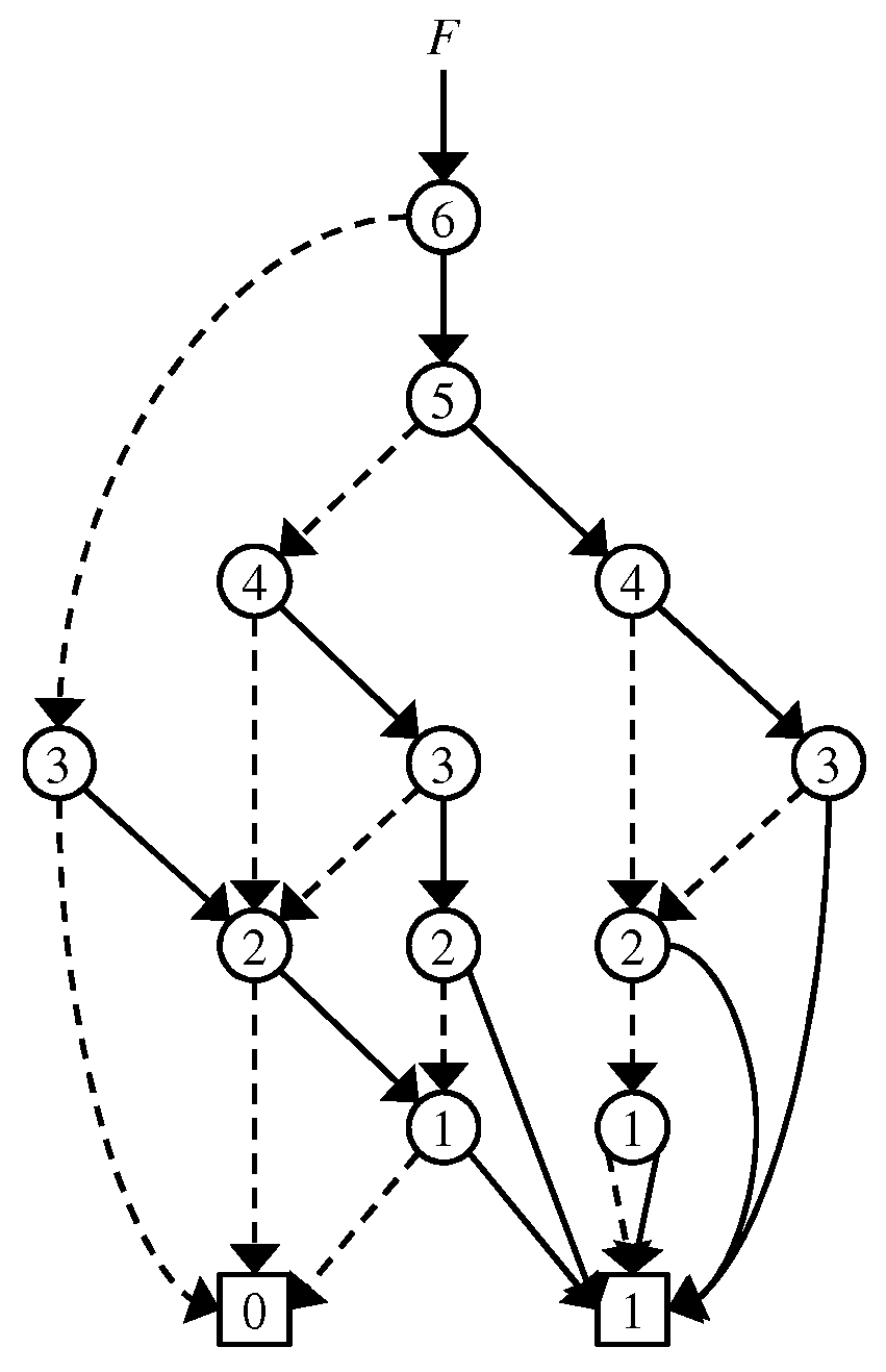
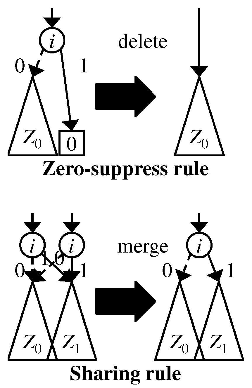
2.3. Zero-Suppressed Binary Decision Diagrams

A zero-suppressed binary decision diagram (ZDD) [2] is a variant of a binary decision diagram [1], customized to manipulate finite families of sets. A ZDD is a directed acyclic graph satisfying the following. A ZDD has two types of nodes, terminal and nonterminal nodes. A terminal node v has as an attribute a value $\mathit{value}(v)\in \{0,1\}$, indicating whether it is the 0-terminal node or the 1-terminal node, denoted by $\mathbf{0}$ and $\mathbf{1}$, respectively. A nonterminal node v has as attributes an integer $\mathit{index}(v)\in \{1,\dots ,n\}$ called the index, and two children $\mathit{zero}(v)$ and $\mathit{one}(v)$, called the 0-child and 1-child. The edge from a nonterminal to its 0-child (1-child resp.) is called the 0-edge (1-edge resp.). In the figures in the paper, terminal and nonterminal nodes are drawn as squares and circles, respectively, and 0-edges and 1-edges are drawn as dotted and solid arrows, respectively. We define $\mathit{triple}(v)=⟨\mathit{index}(v),\mathit{zero}(v),\mathit{one}(v)⟩$, called the attribute triple of v. For any nonterminal node v, $\mathit{index}(v)$ is larger than the indices of its children (In ordinary BDD or ZDD papers, the indices are in ascending order from roots to terminals. For convenience, we employ the opposite ordering in this paper).We define the size of a ZDD G as the number of its nonterminals and denote it by $\left|G\right|$.

Definition 1 (set family represented by a ZDD).

A ZDD $G=(V,E)$ rooted at a node $v\in V$ represents a finite family of sets $F(v)$ on $U_n$ defined recursively as follows: (1) If v is a terminal node: $F(v)=\{\varnothing \}$ if $\mathit{value}(v)=1$, and $F(v)=\varnothing$ if $\mathit{value}(v)=0$. (2) If v is a nonterminal node, then $F(v)$ is the finite family of sets $F(v)=(\left\{\left\{e_{\mathit{index}(v)}\right\}\right\}\bigsqcup F(\mathit{one}(v)))\cup F(\mathit{zero}(v))$.

The example in Figure 1 represents a family of sets $F=\{$ $\{6,5,4,3\}$, $\{6,5,4,2\}$, $\{6,5,4,1\}$, $\{6,5,4\}$, $\{6,5,2\}$, $\{6,5,1\}$, $\{6,5\}$, $\{6,4,3,2\}$, $\{6,4,3,1\}$, $\{6,4,2,1\}$, $\{6,2,1\}$, $\{3,2,1\}$ }. A set $S=\{c_1,\dots ,c_{\ell }\}$ describes a path in the graph G starting from the root in the following way: At each nonterminal node with label $c_i$, the path continues to the 0-child if $c_i\notin S$ and to the 1-child if $c_i\in S$, and the path eventually reaches the 1-terminal (0-terminal resp.), indicating that S is accepted (rejected resp).

Figure 1. Example of ZDD.

We employ the following two reduction rules, shown in Figure 2, to compress ZDDs: (a) Zero-suppress rule: A nonterminal node whose 1-child is the 0-terminal node is deleted; (b) sharing rule: two or more nonterminal nodes having the same attribute triple are merged. By applying the above rules, we can reduce the size of the graph without changing its semantics. If we apply the two reduction rules as much as possible, then we obtain the canonical form for a given family of sets. We implement the sharing rule by using a hash table such that a key is an attribute triple and the value of the key is the pointer to the node corresponding to the attribute triple. When we want to create a new node with an attribute triple $⟨i,v_0,v_1⟩$, we check whether such a node has already existed or not. If such a node exists, we do not create a new node and use the node. Otherwise, we create a new node v with $⟨i,v_0,v_1⟩$ and we register it to the hash table. After that, V and E are updated to $V\cup \left\{v\right\}$ and $E\cup \{(v,v_0),(v,v_1)\}$, respectively.

Figure 2. Reduction rules of ZDDs.

We can further reduce the size of ZDDs by using a type of attributed edges [2,10], named 0-element edges. A ZDD with 0-element edges is defined as follows. A ZDD with 0-element edges has the same property as an ordinary ZDD, except that it does not have the 1-terminal and that the 1-edge of each nonterminal node has as an attribute a one bit flag, called ∅-flag. The ∅-flag of the 1-edge of each nonterminal node v is denoted by $\mathit{empflag}(v)$, whose value is 0 or 1.

Definition 2 (set family represented by a ZDD with 0-element edges).

A ZDD with 0-element edges $G=(V,E)$ rooted at a node $v\in V$ represents a finite family of sets $F(v)$ on $U_n$ defined recursively as follows: (1) If v is the terminal node (note that this means $\mathit{value}(v)=0$): $F(v)=\varnothing$; (2) If v is a nonterminal node and $\mathit{empflag}(v)=1$, then $F(v)$ is the finite family of sets $F(v)=(\left\{\left\{e_{\mathit{index}(v)}\right\}\right\}\bigsqcup (F(\mathit{one}(v))\cup \{\varnothing \})\cup F(\mathit{zero}(v))$; (3) If v is a nonterminal node and $\mathit{empflag}(v)=0$, then $F(v)$ is the finite family of sets $F(v)=(\left\{\left\{e_{\mathit{index}(v)}\right\}\right\}\bigsqcup F(\mathit{one}(v)))\cup F(\mathit{zero}(v))$.

In the figures in this paper, ∅-flags are drawn as small circles at the starting points of 1-edges. Throughout this paper, we always use ZDDs with 0-element edges and simply call it ZDDs. We always denote by m the number of nodes of a given ZDD. An example of a ZDD with 0-element edges is shown in Figure 3. When we use ZDDs with 0-element edges, we employ a pair $⟨v,c⟩,v\in V,c\in \{0,1\}$ to point a node instead of only v, considering that a pair $⟨v,c⟩$ represents the family of sets $F=F(v)\cup \{\varnothing \}$ if $c=1$; otherwise $F=F(v)$.

Figure 3. ZDD using 0-element edges that is equivalent to the ZDD in Figure 1.

Table 1 summarizes operations of ZDDs. The upper half shows the primitive operations, while the lower half shows other operations that can be implemented by using the primitive operations. The operations $\mathit{index}(v)$, $\mathit{zero}(v)$, $\mathit{one}(v)$, $\mathit{topset}(v,i)$ and $\mathit{member}(v,S)$ do not create new nodes. Therefore, they are static operations. Note that the operation $\mathit{count}(v)$ does not create any node; however, we need an auxiliary array to memorize which nodes have already been visited.

Table 1. Main operations supported by ZDD. The first group are the primitive ZDD operations used to implement the others, yet they could have other uses.

$\mathit{index}(v)$	Returns the index of node v.
$\mathit{zero}(v)$	Returns the 0-child of node v.
$\mathit{one}(v)$	Returns the 1-child of node v.
$\mathit{getnode}(i,v_0,v_1)$	Generates (or makes a reference to) a node v
	with index i and two child nodes $v_0=\mathit{zero}(v)$ and $v_1=\mathit{one}(v)$.
$\mathit{topset}(v,i)$	Returns a node with the index i reached by traversing only 0-edges from v.
	If such a node does not exist, it returns the 0-terminal node.
$\mathit{member}(v,S)$	Returns $\mathit{true}$ if $S\in F(v)$, and returns $\mathit{false}$ otherwise.
$\mathit{count}(v)$	Returns $|F(v)|$.
$\mathit{sample}(v)$	Returns a set $S\in F(v)$ uniformly and randomly.
$\mathit{offset}(v,i)$	Returns u such that $F(u)=\{S\subseteq U_n|S\in F,e_i\notin S\}$.
$\mathit{onset}(v,i)$	Returns u such that $F(u)=\{S\backslash \left\{e_i\right\}\subseteq U_n|S\in F,e_i\in S\}$.
${\mathit{apply}}_{\diamond }(v_1,v_2)$	Returns v such that $F(v)=F(v_1)\diamond F(v_2)$, for $\diamond \in \{\cup ,\cap ,\backslash ,\oplus \}$.

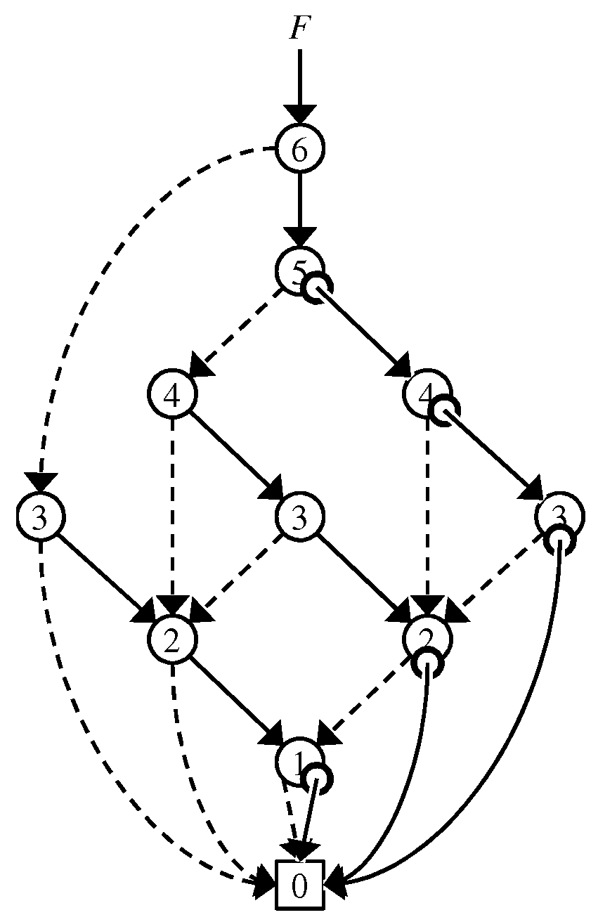
2.4. Problem of Existing ZDDs

Existing ZDD implementations (supporting dynamic operations) have the following problem in addition to the size of representations discussed in Section 1. The $\mathit{member}(v,S)$ operation needs $\mathsf{\Theta }(n)$ time in the worst case. In practice, the sizes of query sets are often much smaller than n, so an $\mathcal{O}(|S|)$ time algorithm is desirable. Existing implementations need $\mathsf{\Theta }(n)$ time for the $\mathit{member}(v,S)$ operation because it is implemented by repeatedly using the $\mathit{zero}(v)$ operation.

For example, we traverse 0-edges 255 times when we search $S=\left\{e_1\right\}$ on the ZDD for $F=\{\left\{e_1\right\},\dots ,\left\{e_{256}\right\}\}$. If we translate the ZDD to an equivalent automaton by using an array to store pointers (see Figure 4), we can execute the searching in $\mathcal{O}(|S|)$ time. ZDD nodes correspond to labeled edges in the automaton. However, the size of such an automaton via straightforward translation can be $\mathsf{\Theta }(n)$ times larger than the original ZDD [11] in the worst case. Therefore, we want to perform $\mathit{member}(v,S)$ operations in $O(|S|)$ time on ZDDs.

Figure 4. Worst-case example of a straightforward translation.

Minato proposed Z-Skip Links [12] to accelerate the traversal of ZDDs of large-scale sparse datasets. Their method adds one link per node to skip nodes that are concatenated by 0-edges. Therefore, the amount of memory requirement cannot be smaller than original ZDDs. Z-Skip-Links make the membership operations much faster than using conventional ZDD operations when handling large-scale sparse datasets. However, the computation time is probabilistically analyzed only for the average case.

3. Data Structure

3.1. DenseZDD

In this subsection, we are going to show what DenseZDD is for a given ZDD Z. We define a DenseZDD for Z as $DZ(Z)=⟨U,M,I⟩$, which consists of the BP U of a zero-edge tree, the bit vector M to indicate dummy nodes, and the integer array I to store one-children.

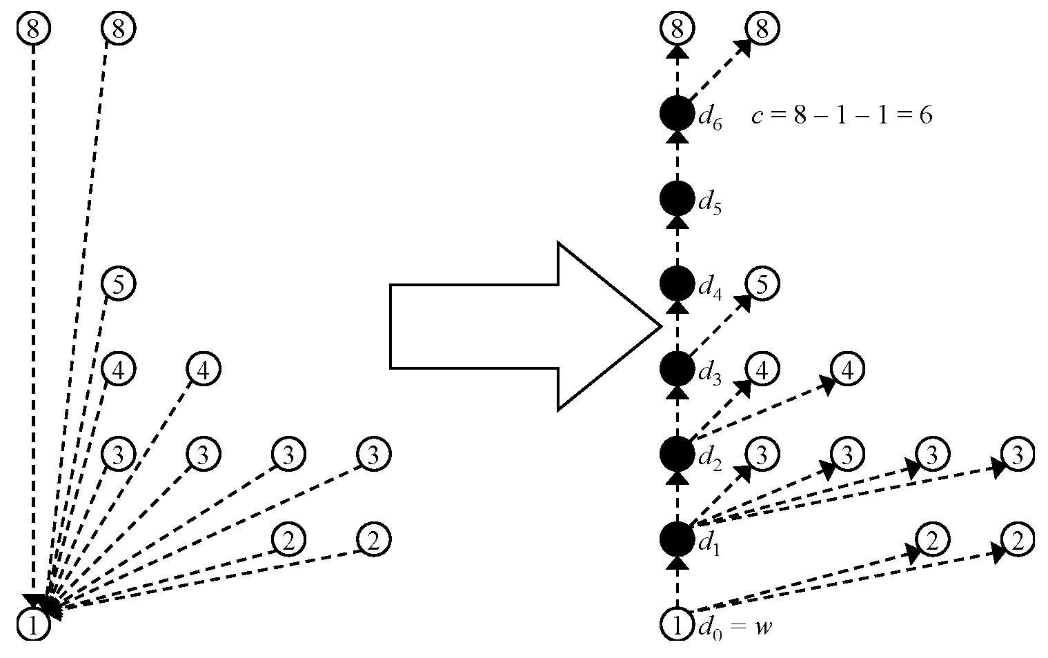
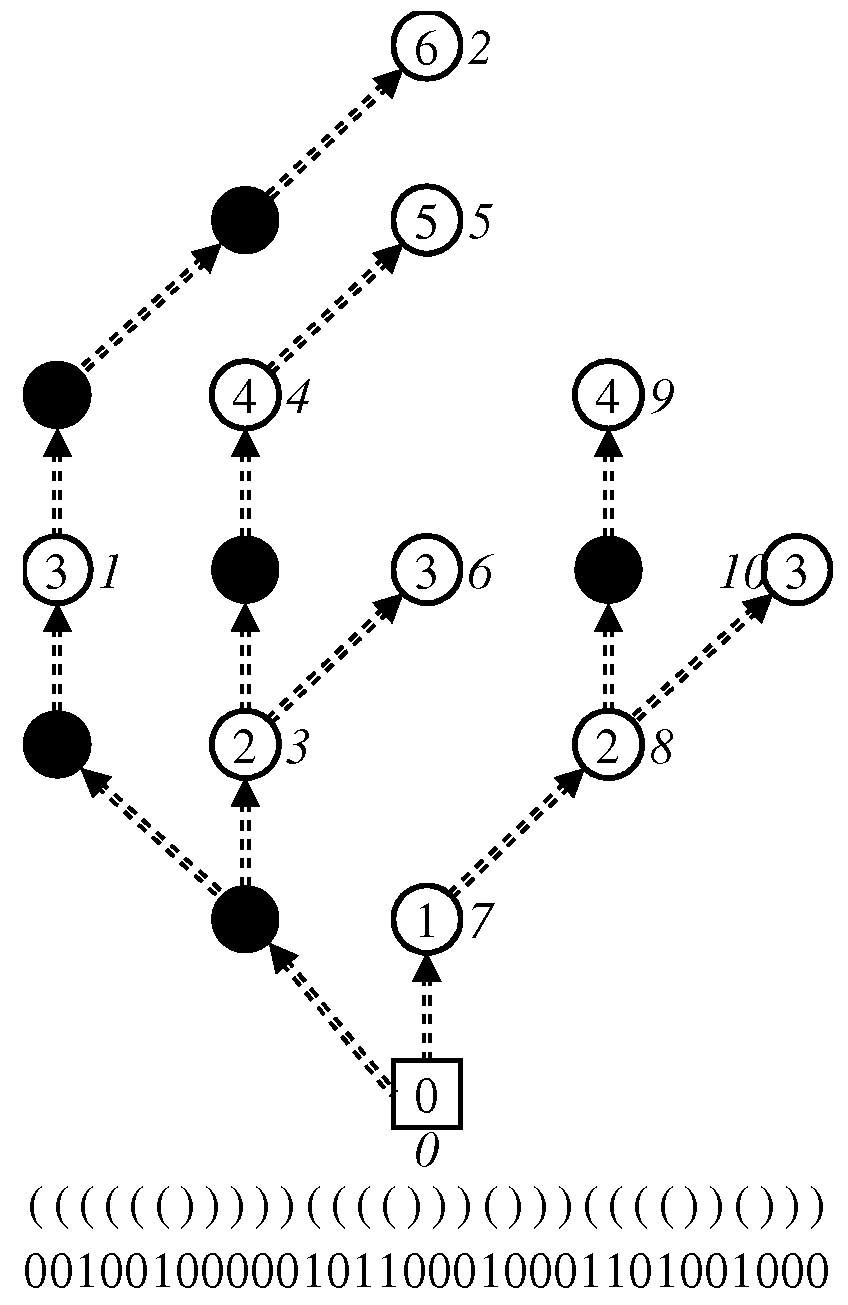
3.1.1. Zero-Edge Tree

We construct the zero-edge tree from a given ZDD G as follows. First of all, we delete all the 1-edges of G. Then, we reverse all the 0-edges, that is, if there is a (directed) edge from v to w, we delete the edge and create the edge from w to v. Note that the tree obtained by this procedure is known as the left/right tree of a DAG whose nodes have two distinguishable arcs, originally used for representing a context-free grammar [13]. We also note that the obtained tree is a spanning one whose root node is the 0-terminal node. Next, we insert dummy nodes into 0-edges so that the distance from the 0-terminal to every node is $\mathit{index}(v)$. Specifically, for each node w that is pointed by 0-edges $(v_1,w),\dots ,(v_k,w)$ in G, we add c dummy nodes $d_1,\dots ,d_c$ and edges $(w,d_1),(d_1,d_2),\dots ,(d_{c-1},d_c)$ and $(d_{b_1},v_1),\dots ,(d_{b_k},v_k)$ to the tree (and remove $(v_1,w),\dots ,(v_k,w)$), where $b_j=\mathit{index}(v_j)-\mathit{index}(w)-1$ for $j=1,\dots ,k$, $c={\max }_{v\in \{v_1,\dots ,v_k\}}\mathit{index}(v)-\mathit{index}(\mathit{w})-1$ and $d_0=w$. If $c=0$, we add no dummy node for the 0-edges pointing at w. For example, see Figure 5.

Figure 5. Example of the construction of the zero-edge tree from a ZDD by inserting dummy nodes and adding/deleting edges. A black and white circle represents a dummy and real node, respectively. The number in a circle represents its index. A dotted arrow in the left figure represents a 0-edge.

We call the resulting tree the zero-edge tree of G and denote it by $T_Z$. To avoid confusion, we call the nodes in $T_Z$ except for dummy nodes real nodes. We construct the BP of $T_Z$ and denote it by U. We let U be the first element of the DenseZDD triplet (described in the beginning of this section).

We define the real preorder rank of a real node v in $T_Z$ (and the corresponding node in G) as the preorder rank of v in the tree before adding dummy nodes and edges connecting nodes.

On BP U, as we will show later, introducing dummy nodes enable to simulate the $\mathit{index}$ and $\mathit{topset}$ operations in constant time by using the $\mathit{depth}$ or $\mathit{level}\_\mathit{ancestor}$ operation of BP. The length of U is $\mathcal{O}(mn)$ because we create at most $n-1$ dummy nodes per one real node. The dummy nodes make the length of U$\mathcal{O}(n)$ times larger, whereas this technique saves $\mathcal{O}(m\log n)$ bits because we do not store the index of each node explicitly.

An example of a zero-edge tree and its BP are shown in Figure 6. Black circles are dummy nodes and the number next to each node is its real preorder rank.

Figure 6. Zero-edge tree and a dummy node vector obtained from the ZDD in Figure 3.

3.1.2. Dummy Node Vector

A bit vector of the same length as U is used to distinguish dummy nodes and real nodes. We call it the dummy node vector of $T_Z$ and denote it by $B_D$. The i-th bit is 1 if and only if the i-th parenthesis of U is ‘(’ and its corresponding node is a real node in $T_Z$. An example of a dummy node vector is also shown in Figure 6. We construct the FID of $B_D$ and denote it by M. We let M be the second element of the DenseZDD triplet. Using M, as we will show later, we can determine whether a node is dummy or real, and compute real preorder ranks in constant time. Moreover, for a given real preorder rank i, we can compute the position of ‘(’ on U that corresponds to the node with real preorder rank i in constant time.

3.1.3. One-Child Array

We now construct an integer array to indicate the 1-child of each nonterminal real node in G by values of real preorder ranks. We call it the one-child array and denote it by $C_O$. More formally, for $i=1,\dots ,m$, $C_O\left[i\right]=v$ means the following: Let $w_T$ be the real node with real preorder rank i in $T_Z$, $w_G$ be the node corresponding to $w_T$ in G, $w_{G1}$ be the 1-child of $w_G$, and $w_{T1}$ be the node corresponding to $w_{G1}$ in $T_Z$. Then, $C_O\left[i\right]=v$ means that the real preorder rank of $w_{T1}$ is the absolute value of v and $\mathit{empflag}(v)=0$ if $v>0$; otherwise $\mathit{empflag}(v)=1$. An example of a one-child array is shown in Figure 7.

Figure 7. One-child array obtained from the ZDD in Figure 3.

As an implementation of $C_O$, we use the fixed length array of integers (see e.g., [14]). We denote it by I. In I, one integer is represented by $\lceil \log (m+1)\rceil +1$ bits, including one bit for the ∅-flag. We let I be the third element of the DenseZDD triplet.

DenseZDD solves the problems as described in Section 2.4. The main results of the paper are the following two theorems.

Theorem 1.

A ZDD Z with m nodes on n items can be stored in $2u+m\log m+3m+o(u)$ bits so that the primitive operations except $\mathit{getnode}(i,v_0,v_1)$ are done in constant time, where u is the number of real and dummy nodes in the zero edge tree of $DZ(Z)$.

Theorem 2.

A ZDD with m nodes on n items can be stored in $\mathcal{O}(m(\log m+\log n))$ bits so that the primitive operations are done in $\mathcal{O}(\log m)$ time except $\mathit{getnode}(i,v_0,v_1)$.

The proofs are given in Section 5. The time complexity of $\mathit{getnode}(i,v_0,v_1)$ is discussed in Section 6.

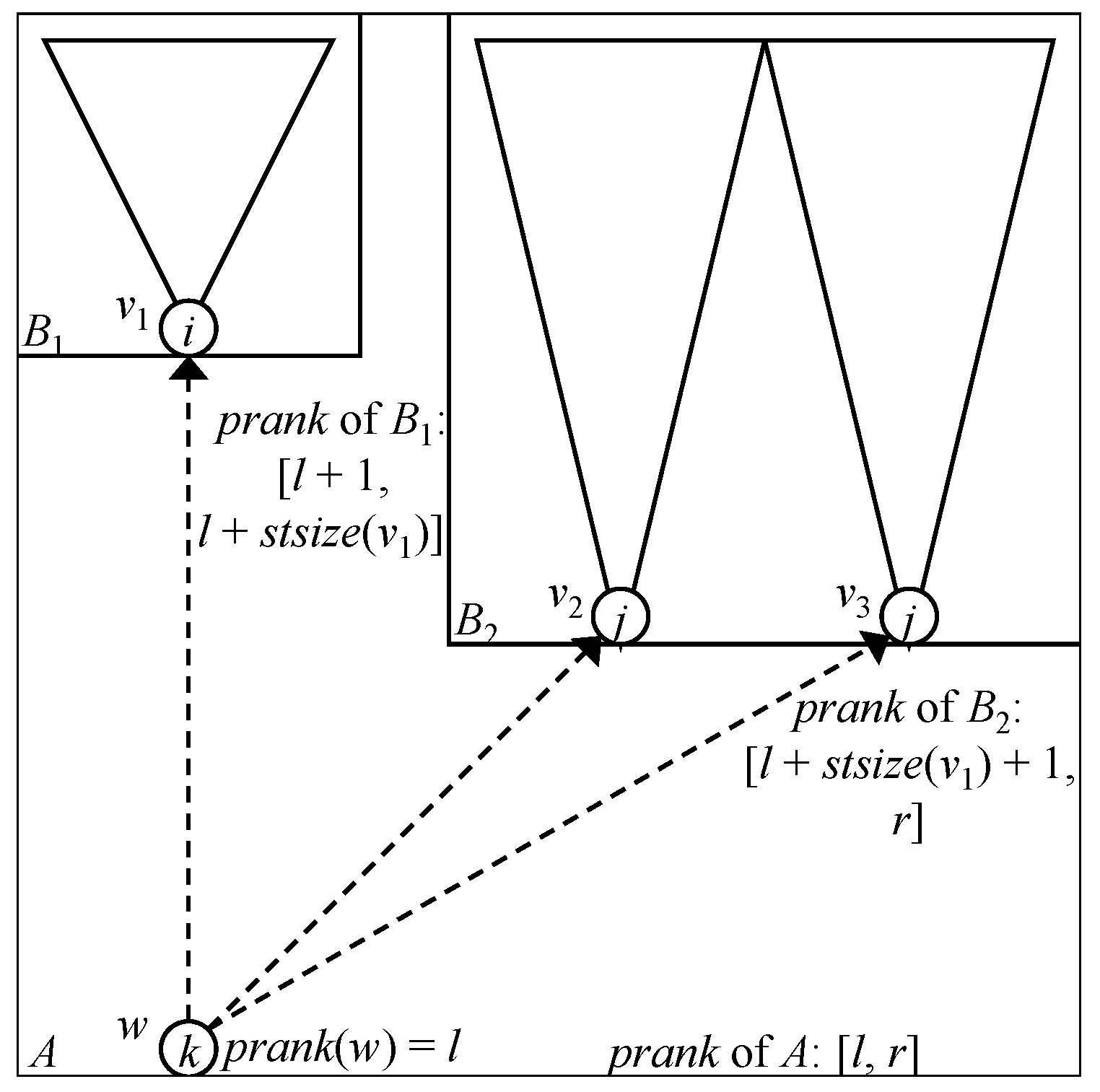
3.2. Convert Algorithm

We show our algorithm to construct the DenseZDD $DZ$ from a given ZDD G in detail. The pseudo-code of our algorithm is given in Algorithm 6. First, we describe how to build the zero-edge tree from G.

The zero-edge tree consists of all 0-edges of the ZDD, with their directions being reversed. For a nonterminal node v, we say that v is a $0^{\mathrm{r}}$-child of $\mathit{zero}(v)$. To make a zero-edge tree, we prepare a list ${\mathit{revzero}}_v$ for each node v, which stores $0^{\mathrm{r}}$-children of the node v. For all nonterminal nodes v, we visit v by a depth-first traversal of the ZDD and add v to ${\mathit{revzero}}_{\mathit{zero}(v)}$. This is done in $\mathcal{O}(m)$ time and $\mathcal{O}(m)$ space because each node is visited at most twice and the total size of ${\mathit{revzero}}_v$ for all v is the same as the number of nonterminal nodes.

Let T be the zero-edge tree before introducing dummy nodes. Let us introduce an order of the elements in ${\mathit{revzero}}_v$ for each v in T so that the $\mathit{getnode}$ operation, described later, can be executed efficiently. Note that the preorder ranks of nodes in T are determined by the order of children of every node in T.

Here, we observe the following fact. Consider a node v in T, and suppose that v has $0^{\mathrm{r}}$-children $v_1,\dots ,v_k$, which are ordered as $v_1<\cdots <v_k$. Let $\mathit{stsize}(v)$ be the subtree size of a node v in T. Then, if the preorder rank of v is p, that of $v_i$ is $p+{\sum }_{j=1}^{i-1}\mathit{stsize}(v_j)+1$ for $i=1,\dots ,k$. Note that, even if the order of $v_1,\dots ,v_{i-1}$ is not determined (it is only determined that $v_i$ is located in the i-th position), the preorder rank of $v_i$, $p+{\sum }_{j=1}^{i-1}\mathit{stsize}(v_j)+1$, can be computed (see Figure 8).

Figure 8. Computing real preorder ranks from the 0-terminal node to real nodes with higher indices.

Now, we introduce an order of the elements in ${\mathit{revzero}}_v$ for each node v. First, for each node v, we order the elements in ${\mathit{revzero}}_v$ in the descending order of their indices. If the indices of two nodes are the same, we temporarily and arbitrarily determine their order (we will change the order later). Then, we do the following procedure for $i=1,\dots ,n$. In the i-th procedure, suppose that the preorder ranks of all the nodes with index smaller than i have already been determined. We consider a node v. Let $\{v_1,\dots ,v_p\}$, $\{v_{p+1},\dots ,v_{p+q}\}$ and $\{v_{p+q+1},\dots ,v_{p+q+r}\}$ be the sets of nodes with index larger than i, equals to i, and smaller than i in ${\mathit{revzero}}_v$, respectively. By our assumption, $v_{p+q+1},\dots ,v_{p+q+r}$ have already been ordered and we now determine the order of $v_{p+1},\dots ,v_{p+q}$. We let the order of $v_{p+1},\dots ,v_{p+q}$ be the descending order of the preorder ranks of their one-children. Note that the preorder ranks of the one-children of $v_{p+1},\dots ,v_{p+q}$ have already been determined. Thus, since the positions of $v_{p+1},\dots ,v_{p+q}$ in ${\mathit{revzero}}_v$ are determined, the above observation implies that the preorder ranks of $v_{p+1},\dots ,v_{p+q}$ are also determined. We do it for all nodes v. After the procedure is finished, the preorder ranks of all the nodes (that is, the order of the children of nodes in T) are determined. As a result, the $0^{\mathrm{r}}$-children $v^{\prime }$ of each node are sorted in the lexicographical order of $⟨\mathit{index}(v^{\prime }),\mathit{prank}(\mathit{one}(v^{\prime }))⟩$. The pseudo-code is given in Algorithm 1.

Algorithm 1 Compute_Preorder: Algorithm that computes the preorder rank $\mathit{prank}(v)$ of each node v. Sets of nodes are implemented by arrays or lists in this code.

1: $L_0\leftarrow \left\{⟨\left\{\mathbf{0}\right\},[0,\mathit{stsize}(\mathbf{0})-1]⟩\right\}$ 2: $L_1,\dots ,L_n$ are lists that are empty initially. 3: for$i=0,\dots ,n$do                ▹$L_i$ includes sets of nodes that have the same index 4:     for each $⟨A,[l,r]⟩\in L_i$ in arbitrary order do            ▹A is a set of nodes that have the same index and 0-child        ▹ Note that $\mathit{prank}$ of nodes with indices less than i are already computed 5:         for each $v\in A$ in descending order of $\mathit{prank}(one(v))$ do 6:            $\mathit{prank}(v)\leftarrow l$; 7:            $l\leftarrow l+1$; 8:            for each $j\in \left\{j\right|w\in \mathit{revzero}(v),j=\mathit{index}(w)\}$ in descending order do 9:                $B\leftarrow \left\{w\right|w\in \mathit{revzero}(v),\mathit{index}(w)=j\}$; 10:                $r\leftarrow l+\mathsf{sum}\{\mathit{stsize}(\mathit{w})|w\in B\}$; 11:                append $⟨B,[l,r]⟩$ to $L_j$;                ▹ That is, the $\mathit{prank}$ of descendants of nodes in B are in $[l,r]$. 12:                $l\leftarrow r+1$; 13:            end for 14:         end for 15:     end for 16: end for 17: return;

To compute $\mathit{prank}$ efficiently, we construct the temporary BP for the zero-edge tree. Using the BP, we can compute the size of each subtree rooted by v in T in constant time and compact space. Since we can compute the size of the subtrees in T, we can know the ranges of real preorder ranks that are assigned to the subtrees by bottom-up processing. The whole tree, the subtree rooted by the 0-terminal node, is assigned the range of preorder rank $[0,m]$. Let w be a node rooting a subtree that is assigned a range of real preorder ranks $[l,l+\mathit{stsize}(w)-1]$ and assume that the $\mathit{revzero}(\mathit{w})$ is sorted. Then, the real preorder rank of w is l and the subtree rooted by $v_j\in \mathit{revzero}(w)$ is assigned the range $[l_j,l_{j+1}-1]$, where $l_j=l_{j-1}+\mathit{stsize}(v_j)$ and $l_1=l+1$.

The DenseZDD for the given ZDD G is composed of these three data structures. We traverse T in depth-first search (DFS) order based on assigned real preorder ranks and construct the BP representation U, the dummy node vector M, and the one-child array I. The BP and dummy node vector are constructed as if dummy nodes exist. Finally, we obtain the DenseZDD $DZ(G)=⟨U,M,I⟩$. The pseudo-code is given in Algorithms 2 and 3.

Algorithm 2 Convert_ZDD_BitVectors ($v,paren,dummy,onechild$): Algorithm for obtaining the BP representation of the zero-edge tree, the dummy node vector, and the one-child array.

Input: ZDD node v, list of parentheses $paren$, list of bits $dummy$, list of integers $onechild$ 1: $i=\mathit{index}(v)$; 2: for each$w\in \mathit{revzero}(v)$ in ascending order of $\mathit{prank}(w)$ do 3:     while $i+1\ne \mathit{index}(w)$ do 4:         if $i+1\le \mathit{index}(w)$ then 5:            append ‘(’ to $paren$, and ‘0’ to $dummy$; 6:            $i\leftarrow i+1$; 7:         else 8:            append ‘)’ to $paren$, and ‘0’ to $dummy$; 9:            $i\leftarrow i-1$; 10:         end if 11:     end while 12:     append ‘(’ to $paren$, and ‘1’ to $dummy$; 13:     append $\mathit{prank}(\mathit{one}(w))·(-1^{\mathit{empflag}(w)})$ to $onechild$; 14:     Convert_ZDD_BitVectors $(w,paren,dummy,onechild)$; 15:     append ‘)’ to $paren$, and ‘0’ to $dummy$; 16: end for 17: while$i>\mathit{index}(v)$do 18:     append ‘)’ to $paren$, and ‘0’ to $dummy$; 19:     $i\leftarrow i-1$; 20: end while 21: return;

Algorithm 3 Construct_DenseZDD (W: a set of root nodes of ZDD): Algorithm for constructing the DenseZDD from a source ZDD.

Output: DenseZDD $DZ$ 1: for each$v\in W$ compute $\mathit{revzero}$ fields for all descendants of v; 2: compute $\mathit{stsize}$ field for all $0^{\mathrm{r}}$-decsendants; 3: Compute_Preorder; 4: create empty lists $paren,dummy,onechild$; 5: append ‘(’ to $paren$, and ‘0’ to $dummy$; 6: Convert_ZDD_BitVectors($\mathbf{0}$, paren, dummy, onechild); 7: append ‘)’ to $paren$, and ‘0’ to $dummy$; 8: make BP U from $paren$; 9: make FID M from $dummy$; 10: make compressed representation I of $onechild$; 11: return$DZ\leftarrow ⟨U,M,I⟩$;

4. ZDD Operations

We show how to implement primitive ZDD operations on DenseZDD $DZ=⟨U,M,I⟩$ except $\mathit{getnode}$. We give an algorithm for $\mathit{getnode}$ in Section 6.

We identify each node with its real preorder rank. We can convert the real preorder rank i of a node to the its position p in the BP sequence U, that is, the position of corresponding ‘(’ by $p:={\mathit{select}}_1(M,i)$ and $i:={\mathit{rank}}_1(M,p)$, and vice versa. Algorithms in Table 1 are as follows:

4.1. $\mathit{index}(i)$

Since the index of a node is the same as the depth, i.e., the distance from the 0-terminal node, of the node in the zero-edge tree $T_Z$, we can obtain $\mathit{index}(i):=\mathit{depth}(U,{\mathit{select}}_1(M,i))$.

4.2. $\mathit{topset}(i,d)$

The node $\mathit{topset}(i,d)$ is the ancestor of node i in $T_Z$ with index d. A naive solution is to iteratively climb up $T_Z$ from node i until we reach the node with index d. However, as shown above, the index of a node is identical to its depth. By using the power of the succinct tree data structure, we can directly find the answer by $\mathit{topset}(i,d):={\mathit{rank}}_1(M,\mathit{level}\_\mathit{ancestor}(U,{\mathit{select}}_1(M,i),d))$. If such a node with the index i is not reachable by traversing only 0-edges, the node obtained by $\mathit{topset}(i,d)$ is a dummy node. We check whether the node is a dummy node or not by using the dummy node vector. If the node is a dummy node, we return the 0-terminal node.

4.3. $\mathit{zero}(i)$

Implementing the $\mathit{zero}$ operation requires a more complicated technique. Recall the insertion of dummy nodes when we construct $T_Z$ in Section 3.1. Consider the subtree in $T_Z$ induced by the set of the nodes consisting of the node i, its 0-child w, the dummy nodes $d_1,\dots ,d_c$ between i and w, and the real nodes $v_1,\dots ,v_k$ pointed by $d_1,\dots ,d_c$. Note that one of $v_1,\dots ,v_k$ is i. Without loss of generality, $v_1$ has the smallest real preorder rank (highest index) among $v_1,\dots ,v_k$, and there are edges $(w,d_1),(d_1,d_2),\dots ,(d_{c-1},d_c),(d_c,v_1)$ (see Figure 5). Computing $\mathit{zero}(i)$ is equivalent to finding w. In the BP U of $T_Z$, ’(’s corresponding to $w,d_1,d_2,\dots ,d_{c-1},d_c,v_1$ continuously appear, and the values of them in $B_D$ is $1,0,0,\dots ,0,0,1$, respectively. Noticing that the parent of i is one of $w,d_1,\dots ,d_c$ and that the real preorder rank of a real node is obtained by ${\mathit{rank}}_1(M,r)$ if the position of the corresponding ’(’ is r in U, we obtain $\mathit{zero}(i):={\mathit{rank}}_1(M,\mathit{parent}(U,{\mathit{select}}_1(M,i)))$.

4.4. $\mathit{one}(i)$

The operation $\mathit{one}(i)$ is quite easy. The 1-child of the node i is stored in the i-th element of the one-child array I. Note that the real preorder rank of the 1-child of i is $abs(i)$, where $abs(i)$ is a function to get the absolute value of i. The ∅-flag of i is 1 if $i\le 0$. Otherwise, it is 0.

4.5. $\mathit{count}(i)$

Counting the number of sets in the family represented by the ZDD whose root is a node i, i.e., $|F(i)|$, is implemented by the same algorithm as counting on ordinary ZDDs. The pseudo-code is given in Algorithm 4. It requires an additional array C to store the cardinality of each node (for a node $i^{\prime }$, we call the cardinality of the family represented by the ZDD whose root is the node $i^{\prime }$the cardinality of the node $i^{\prime }$). After we execute this algorithm, $C\left[i\right]$ equals $|F(i)-\{\varnothing \left\}\right|$. The cardinalities are computed recursively. The algorithm $\mathit{count}(i^{\prime })$ is called for each node $i^{\prime }$ only once in the recursion. The time complexity of $\mathit{count}$ is $\mathsf{\Theta }(m)$, where m is the number of nodes.

4.6. $\mathit{sample}(i)$

We propose two algorithms to implement $\mathit{sample}(i)$. The first one is the same algorithm as random sampling on ordinary ZDDs. Before executing these algorithms, we have to run the counting algorithm to prepare the array C that stores the cardinalities of nodes. The pseudo-code is given in Algorithm 5. We begin traversal from a root node of the ZDD that represents a set family F. At each node i, we decide whether or not the index of node i is included in the output set. We know that the number of the sets including $\mathit{index}(i)$ is $C[one(i)]$. We also know that the number of the sets not including $\mathit{index}(i)$ is $C[zero(i)]$. Then, we generate an integer $r\in [0,C[i])$ uniformly and randomly. If $r<C[zero(i)]$, we do not choose $\mathit{index}(i)$ and go to $\mathit{zero}(i)$. Otherwise, we add $\mathit{index}(i)$ to the output set and go to $\mathit{one}(i)$. We continue this process until we reach the 1-terminal node. At last, we obtain a set uniformly and randomly chosen from F. The time complexity of this algorithm is $\mathcal{O}(n)$.

Algorithm 4 Count$(i)$: Algorithm that computes the cardinality of the family of sets represented by nodes reachable from a node i. The cardinalities are stored in an integer array C of length m, where m is the number of ZDD nodes. The initial values of all the elements in C are 0.

1: if$i=0$then 2:     return 0; 3: end if 4: if$C\left[i\right]\ne 0$then 5:     return $C\left[i\right]$; 6: end if 7: $i_0\leftarrow zero(i)$; 8: $car{d}_0\leftarrow \mathbf{Count}(i_0)$; 9: $i_1\leftarrow one(i)$; 10: $car{d}_1\leftarrow \mathbf{Count}(\mathit{abs}(i_1))$; 11: $card\leftarrow car{d}_0+car{d}_1$; 12: if$i_1\le 0$then 13:     $card\leftarrow card+1$; 14: end if 15: $C\left[i\right]\leftarrow card$; 16: return$card$;

Algorithm 5 Random_naive$(i,\mathit{empflag})$: Algorithm that returns a set uniformly and randomly chosen from the family of sets that is represented by a ZDD whose root is node i. Assume that Count has already been executed. The argument $\mathit{empflag}\in \{0,1\}$ means whether or not the current family of sets has the empty set. If $\mathit{empflag}=1$, this family has the empty set.

1: if$i=0$then 2:     return ∅; 3: end if 4: $i_0\leftarrow zero(i)$; 5: $i_1\leftarrow one(i)$; 6: $card\leftarrow C\left[i\right]+\mathit{empflag}$; 7: Generate an integer in $r\in [0,card)$ uniformly and randomly. 8: if$r<C\left[i_0\right]+\mathit{empflag}$then 9:     return Random_naive $(i_0,\mathit{empflag})$ 10: else 11:     if $i_1\le 0$ then 12:         $e\leftarrow 1$; 13:     else 14:         $e\leftarrow 0$; 15:     end if 16:     return $\{\mathit{index}(i)\}\cup$ Random_naive $(abs(i_1),e)$; 17: end if

The second algorithm is based on binary search. The main idea of this algorithm is that we consider multiple nodes at once whose indices are possibly chosen as the next element of the output set. The pseudo-code is given in Algorithm 6. As well as the first algorithm, we begin traversal from a root node. Note that the first element of the output set is one of the indices of the nodes that are reachable only by 0-edges from the current node. We use $\mathit{topset}$ operation to decide which index of a node is chosen. Let the current node be i. We execute binary search on these nodes. As an initial state, we consider the range $(l=-1,h=\mathit{index}(i)]$ as candidates. Next, we divide this range by finding a node with index less than or equal to $c=\lfloor l+h+1\rfloor /2$. Such a node can be found by $\mathit{topset}(i,c)$. Recall that $\mathit{topset}(i,d):={\mathit{rank}}_1(M,\mathit{level}\_\mathit{ancestor}(U,{\mathit{select}}_1(M,i),d))$. It is the real preorder rank of a node whose index is less than c or equal to c. If the index of the found node is less than or equal to l, we update l by $l\leftarrow c$ and repeat the execution of $\mathit{topset}$. When a node with index x, $l<x\le h$, is found, we choose either $(l,c]$ or $(c,h]$ as a next candidate range for further binary search. We know the cardinality of nodes with indices h, c, and l. The cardinality $card$ of the family of sets we consider now is the cardinality of the node with index h minus the cardinality of the node with index l. Then, generate a random integer $r\in [0,card)$. If r is less than the cardinality of the node with index c, update h by $h\leftarrow c$. Otherwise, update l by $l\leftarrow c$. We continue this procedure until $l+1=h$. After that, we choose the index h as an element of the output set, and go to the 1-child of the node with index h. Again, we start binary search on the next nodes connected by continuous 0-edges. This algorithm stops when it reaches the 1-terminal node.

Algorithm 6 Random_bin$(i,\mathit{empflag})$: Algorithm that returns a set uniformly and randomly chosen from the family of sets represented by the ZDD whose root is node i. This algorithm chooses the index by binary search on nodes linked by 0-edges.

1: ${\mathit{idx}}_i\leftarrow \mathit{index}(i)$, $j\leftarrow -1$, ${\mathit{idx}}_j\leftarrow -1$; 2: $car{d}_j=0$; 3: while${\mathit{idx}}_i\ne {\mathit{idx}}_j$do 4:     if ${\mathit{idx}}_i=0$ then 5:         return ∅; 6:     end if 7:     ${\mathit{idx}}_k\leftarrow \lfloor ({\mathit{idx}}_i+{\mathit{idx}}_j+1)/2\rfloor$; 8:     $k\leftarrow \mathit{topset}(i,{\mathit{idx}}_k)$; 9:     if $j=k$ then 10:         $j\leftarrow k$; 11:         continue; 12:     end if 13:     Generate an integer $r\in [0,C\left[i\right]+\mathit{empflag}-car{d}_j)$ uniformly and randomly. 14:     if $r<C\left[j\right]+\mathit{empflag}-{\mathit{card}}_j$ then                        ▹$({\mathit{idx}}_j,{\mathit{idx}}_k]$ is chosen 15:         $i\leftarrow k$; 16:         ${\mathit{idx}}_i\leftarrow {\mathit{idx}}_k$; 17:     else                        ▹$({\mathit{idx}}_k,{\mathit{idx}}_i]$ is chosen 18:         $j\leftarrow k$; 19:         ${\mathit{idx}}_j\leftarrow {\mathit{idx}}_k$; 20:         ${\mathit{card}}_j\leftarrow {\mathit{card}}_j+C\left[k\right]$; 21:         if $\mathit{empflag}=1$ then 22:            ${\mathit{card}}_j\leftarrow {\mathit{card}}_j-1$; 23:            $\mathit{empflag}\leftarrow 0$; 24:         end if 25:     end if 26: end while 27: $i_1\leftarrow \mathit{one}(i)$; 28: if$i_1\le 0$then 29:     return $\left\{{\mathit{idx}}_i\right\}\cup$ Random_bin $(abs(i_1),1$); 30: else 31:     return $\left\{{\mathit{idx}}_i\right\}\cup$ Random_bin $(abs(i_1),0$); 32: end if

This algorithm takes $\mathcal{O}(\log n)$ time to choose one element of an output. The time complexity of this algorithm is $\mathcal{O}(n\log n)$. This looks worse than the previous algorithm. However, this can be better for set families consisting of small sets. Let s be the size of the largest sets in the family. Then, its time complexity is $\mathcal{O}(s\log n)$. Therefore, this algorithm is efficient for large data sets consisting of small sets of many items.

5. Complexity Analysis

Let the length of balanced parentheses sequence U be $2u$, where u is the number of ZDD nodes with dummy nodes. When a ZDD has m nodes and the number of items is n, u is $mn$ in the worst case. Here, we show how to compress the BP sequence U.

We would like to decrease the space used by DenseZDD. However, we added extra data, dummy nodes, to the given ZDD. We want to bound the memory usage caused by dummy nodes. From the pseudo-code in Algorithm 2, we observe that the BP sequence U consists of at most $2m$ runs of identical symbols. To see this, consider the substring of U between the positions for two real nodes. There is a run consisting of consecutive ‘)’ followed by a run consisting of consecutive ‘(’ in the substring. We compress U by using some integer encoding scheme such as the delta-code or the gamma-code [15]. An integer $x>0$ can be encoded in $\mathcal{O}(\log x)$ bits. Since the maximum length of a run is n, U can be encoded in $\mathcal{O}(m\log n)$ bits. The range min-max tree of U has $2m/\log m$ leaves. Each leaf of the tree corresponds to a substring of U that contains $\log m$ runs. Then, any tree operation can be done in $\mathcal{O}(\log m)$ time. The range min-max tree is stored in $\mathcal{O}(m(\log n+\log m)/\log m)$ bits.

We also compress the dummy node vector $B_D$. Since its length is $2u\le 2mn$ and there are only m ones, it can be compressed in $m(2+\log m)+o(u)$ bits by FID. The operations ${\mathit{select}}_1$ and ${\mathit{rank}}_1$ take constant time. We can reduce the term $o(u)$ to $o(m)$ by using a sparse array [16]. Then, the operation ${\mathit{select}}_1$ is done in constant time, while ${\mathit{rank}}_1$ takes $\mathcal{O}(\log m)$ time. We call the DenseZDD whose zero-edge tree and dummy node vector are compressed dummy-compressed DenseZDD.

From the discussion in the section, we can prove Theorems 1 and 2.

Proof of Theorem 1.

From the above discussion, the BP U of the zero-edge tree costs $2u=\mathcal{O}(mn)$ bits, where u is the number of real nodes and dummy nodes. The one-child array needs $m\log m$ bits for 1-children and m bits for ∅-flags. Using FID, the dummy node vector is stored in $m(2+\log m)+o(u)$ bits. Therefore, the DenseZDD can be stored in $2u+3m+2m\log m+o(u)$ bits and the primitive operations except $\mathit{getnode}$ are done in constant time because the ${\mathit{rank}}_1$, ${\mathit{select}}_1$, and any tree operations take constant time by Proposition 1. ☐

Proof of Theorem 2.

When we compress U, it can be stored in $\mathcal{O}(m\log n)$ bits and the min-max tree is stored in $\mathcal{O}(m(\log n+\log m)/\log m)$ bits. The dummy node vector can be compressed in $m(2+\log m)+o(m)$ bits by FID with sparse array. The time of any tree operations and the ${\mathit{rank}}_1$ operation is $\mathcal{O}(\log m)$. Therefore, the DenseZDD can be stored in $\mathcal{O}(m(\log m+\log n))$ bits and the primitive operations except for $\mathit{getnode}$ take $\mathcal{O}(\log m)$ time because all of them use tree operations on U or ${\mathit{rank}}_1$ on M. ☐

6. Hybrid Method

In this section, we show how to implement dynamic operations on DenseZDD. Namely, we implement the $\mathit{getnode}(i,v_0,v_1)$ operation. Our approach is to use a hybrid data structure using both the DenseZDD and a conventional dynamic ZDD. Assume that initially all the nodes are represented by a DenseZDD. Let $m_0$ be the number of initial nodes. In a conventional dynamic ZDD, the operation $\mathit{getnode}(i,v_0,v_1)$ is implemented by a hash table indexed with the triple $⟨i,v_0,v_1⟩$.

We first show how to check whether the node $v:=\mathit{getnode}(i,v_0,v_1)$ has already existed or not. That is, we want to find a node v such that $\mathit{index}(v)=i$, $\mathit{zero}(v)=v_0$, $\mathit{one}(v)=v_1$. If v exists in the zero-edge tree, v is one of the $0^{\mathrm{r}}$-children of $v_0$. Consider again the subtree of the zero-edge tree rooted at $v_0$ and the $0^{\mathrm{r}}$-children of $v_0$ (see the right of Figure 5). Let $d_p$ be the (possibly dummy) parent of v in the zero edge tree. The parent of all the $0^{\mathrm{r}}$-children of $v_0$ with index i in the zero edge tree is also $d_p$. The node $d_p$ is located on the path from $v_0$ to the first node, say $v_{\mathrm{f}}$, among the $0^{\mathrm{r}}$-children of $v_0$ (note that since the zero edge tree is an ordered tree, we can well-define the “first” node). That is, $d_p$ is an ancestor of $v_{\mathrm{f}}$. Since the position of $v_{\mathrm{f}}$ is the next of the position of $v_0$ in M (in the preorder), we can obtain the position of $v_{\mathrm{f}}$ by ${\mathit{select}}_1(M,{\mathit{rank}}_1(M,v_0)+1)$. Noting that the index of $d_p$ is $i-1$, we obtain the position of $d_p$ by $d_p=\mathit{level}\_\mathit{ancestor}(U,{\mathit{select}}_1(M,{\mathit{rank}}_1(M,v_0)+1),i-1)$. Our task is to find the node v such that $\mathit{one}(v)=v_1$ among the children of $d_p$. Since the $0^{\mathrm{r}}$-children $v^{\prime }$ of $d_p$ are sorted in the lexicographic order of $⟨\mathit{index}(v^{\prime }),\mathit{prank}(\mathit{one}(v^{\prime }))⟩$ values by the construction algorithms, we can find v by a binary search. For this, we use the $\mathit{degree}$ and $\mathit{child}$ operations on the zero-edge tree (recall that $\mathit{degree}$ is used for obtaining the number of children of a node).

If v does not exist, we create such a node and register it to the hash table as well as a dynamic ZDD. Note that we do not update the DenseZDD, and thus if we want to treat the ZDD, say $Z_{\mathrm{new}}$, whose root is the new node as the DenseZDD, we need to construct the DenseZDD structure for $Z_{\mathrm{new}}$.

We obtain the following theorem on the time complexity.

Theorem 3.

The existence of $\mathit{getnode}(i,v_0,v_1)$ can be checked in $\mathcal{O}(t\log m)$ time, where t is the time complexity of primitive ZDD operations.

If the BP sequence is not compressed, $\mathit{getnode}$ takes $\mathcal{O}(\log m)$ time; otherwise it takes $\mathcal{O}({\log }^{2}m)$ time. By discussion similar to the proofs of Theorems 1 and 2 in Section 5, we have the following theorems.

Theorem 4.

A ZDD with m nodes on n items can be stored in $2u+m\log m+3m+o(u)$ bits so that the $\mathit{getnode}(i,v_0,v_1)$ operation is done in $\mathcal{O}(\log m)$ time, where u is the number of real and dummy nodes in the zero edge tree of $DZ(Z)$.

Theorem 5.

A ZDD with m nodes on n items can be stored in $\mathcal{O}(m(\log m+\log n))$ bits so that the $\mathit{getnode}(i,v_0,v_1)$ operation is done in $\mathcal{O}({\log }^{2}m)$ time.

7. Other Decision Diagrams

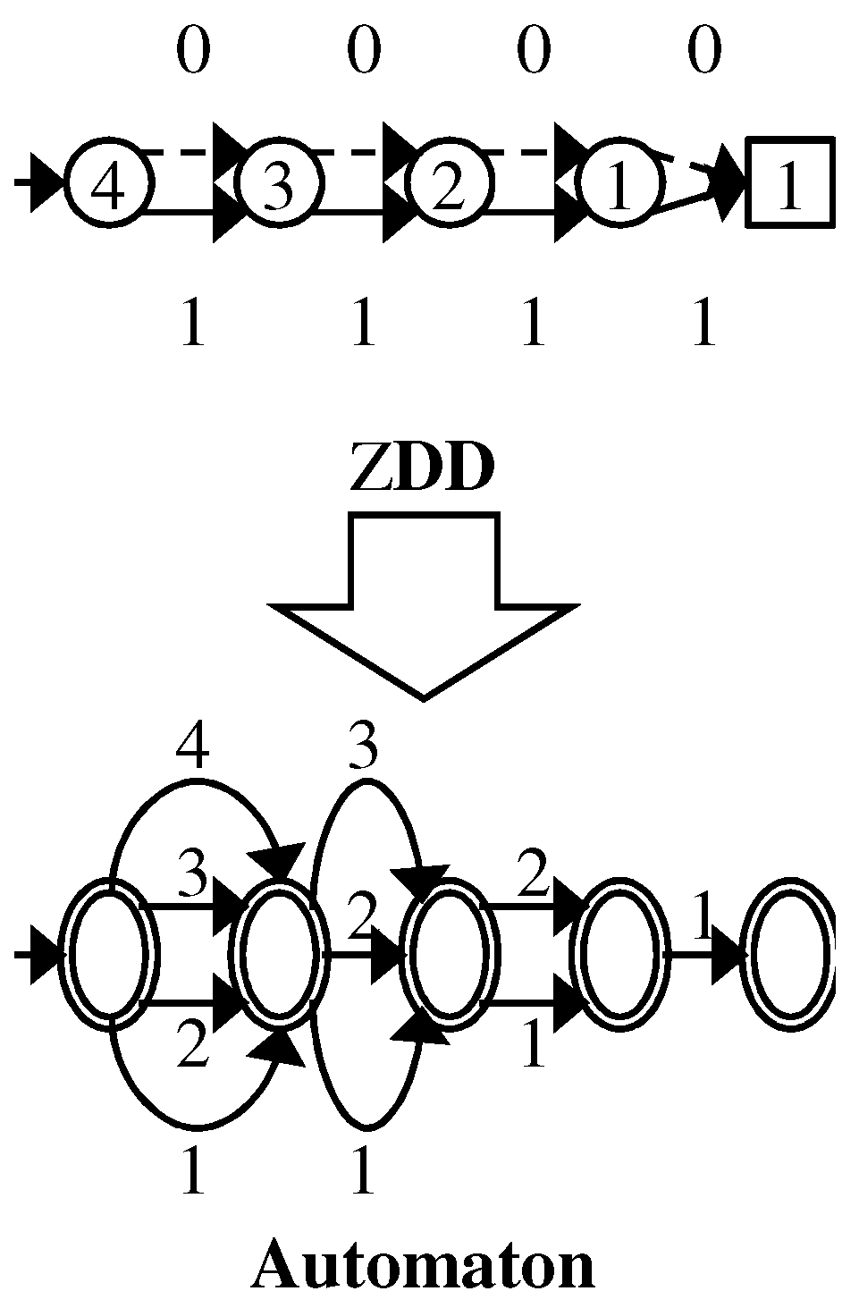
7.1. Sets of Strings

A sequence binary decision diagram (SeqBDD) [17] is a variant of a zero-suppressed binary decision diagram, customized to manipulate sets of strings. The terminology of SeqBDDs is almost the same as that of ZDDs. Let $c_1,\dots ,c_n$ be letters such that $c_1<c_2<\cdots <c_n$ and ${\Sigma }_n=\{c_1,\dots ,c_n\}$ be an alphabet. Let $s=x_1,\dots ,x_l$, $l\ge 0$, $x_1,\dots ,x_{\ell }\in {\Sigma }_n$, be a string. We denote the length of s by $\left|s\right|=\ell$. The empty string is denoted by $\epsilon$. The concatenation of strings $s=x_1,\dots ,x_{{\ell }_1}$ and $t=y_1,\dots ,y_{{\ell }_2}$ is defined as $s·t=x_1,\dots ,x_{{\ell }_1},y_1,\dots ,y_{{\ell }_2}$. The product of string sets $L_1$ and $L_2$ is defined as $L_1\times L_2=\{s_1·s_2|s_1\in L_1,s_2\in L_2\}$.

A SeqBDD is a directed acyclic graph. The difference between SeqBDD and ZDD is a restriction for indices of nodes connected by edges. For any SeqBDD nonterminal node v, the index of v’s 0-child must be smaller than that of v, but the index of v’s 1-child can be larger than or equal to that of v. This relaxation is required to represent string sets because a string can have the same letters at multiple positions. The definition of SeqBDDs is the following:

Definition 3 (string set represented by a SeqBDD).

A SeqBDD $G=(V,E)$ rooted at a node $v\in V$ represents a finite sets of strings $L(v)$ whose letters are in ${\Sigma }_n$ defined recursively as follows: (1) If v is a terminal node: $L(v)=\left\{\epsilon \right\}$ if $\mathit{value}(v)=1$, and $L(v)=\varnothing$ if $\mathit{value}(v)=0$; (2) If v is a nonterminal node, then $L(v)$ is the finite set of strings $L(v)=(\left\{\left\{c_{\mathit{index}(v)}\right\}\right\}\times L(\mathit{one}(v)))\cup L(\mathit{zero}(v))$.

A string $s=x_1,\dots ,x_{\ell }$ describes a path in the graph G starting from the root in the same way as ZDDs. For SeqBDDs, we also employ the zero-suppress rule and the sharing rule. By applying these rules as much as possible, we can obtain the canonical form for given sets of strings.

We can compress SeqBDDs by the same algorithm as the DenseZDD construction algorithm. We call it DenseSeqBDD. Since the index restriction between nodes connected by 0-edges is still valid on SeqBDDs, we can represent indices of nodes and connection by 0-edges among nodes by zero-edge trees. The main operations of SeqBDD such as $\mathit{index}$, $\mathit{zero}$, $\mathit{one}$, $\mathit{topset}$, $\mathit{member}$, $\mathit{count}$, and $\mathit{sample}$ are also implemented by the same algorithms. Recall that a longest path on a ZDD is bounded by the number of items n. Therefore, the time complexities of $\mathit{member}$ and $\mathit{sample}$ on a ZDD are at most $\mathcal{O}(n)$, which means that the benefit we can gain by skipping continuous 0-edges in $\mathit{topset}$ algorithm is not so large because the total number of nodes we can skip is less than n. However, a longest path on a SeqBDD is not bounded by the number of letters, and thus we can gain more benefit of skipping 0-edges because indices of nodes reached after traversing 1-edges can be the largest index. The time complexities of $\mathit{member}$ and $\mathit{sample}$ on a SeqBDD are $\mathcal{O}(\mathit{maxlen})$ and $\mathcal{O}(\mathit{maxlen}\log |{\Sigma }_n|)$, respectively, where $\mathit{maxlen}$ is the length of the longest string included in the SeqBDD.

7.2. Boolean Functions

In the above subsection, we applied our technique to decision diagrams for sets of strings. Next, we consider another decision diagram for Boolean functions, BDD. Is it possible to compress BDDs by the same technique, and are operations fast on such compressed BDDs? The answer to the first question is “Yes”, but to the second question is “No”. Since a BDD is also a directed acyclic graph consisting of two terminal nodes and nonterminal nodes with distinguishable two edges, the structure of a BDD can be represented by the zero-edge tree, dummy node vector, and one-child array. Therefore, we can obtain a compressed representation of a BDD. On the other hand, the membership operation on a ZDD corresponds to the operation to determine whether or not an assignment of Boolean variables satisfies the Boolean function represented by a BDD. Since the size of query for the assignment operation is always the number of all Boolean variables, we cannot skip any assignment to variables. As a result, membership operation and random sampling operation are not accelerated on a BDD even if we use the DenseZDD technique.

8. Experimental Results

We ran experiments to evaluate the compression, construction, and operation times of DenseZDDs. We implemented the algorithms described in Section 3 and Section 3.2 in C/C++ languages on top of the SAPPORO BDD package, which is available at https://github.com/takemaru/graphillion/tree/master/src/SAPPOROBDD and can be found as an internal library of Graphillion [18]. The package uses 32 bytes per ZDD node. The breakdown of 32 bytes of a ZDD node is as follows: 5 bytes as a pointer for the 1-child, 5 bytes as a pointer for the 0-child, 2 bytes as an index. In addition, we use a closed hash table to execute $\mathit{getnode}$ operation. The size of the hash table of SAPPOROBDD is $5\times 2\times n$ bytes, and 5 bytes per each node to chain ZDD nodes that have the same key computed from its attribute-triple. Since DenseZDD does not require such hash table to execute $\mathit{getnode}$, we consider that the space used by the hash table should be included in the memory consumption of ZDD nodes. The experiments are performed on a machine with 3.70 GHz Intel Core i7-8700K and 64 GB memory running Windows Subsystem for Linux (Ubuntu) on Windows 10.

We show the characteristics of the data sets in Table 2. As artificial data sets, we use rectrxw, which represents families of sets ${⨆}_{i=0}^{r-1}\{\{iw+1\},\dots ,\{iw+w\}\}$. Data set randomjoink is a ZDD that represents the join $C_1\bigsqcup \cdots \bigsqcup C_4$ of four ZDDs for random families $C_1,\dots ,C_4$ consisting of k sets of size one drawn from the set of $n=32768$ items. Data set bddqueenk is a ZDD that stores all solutions for k-queen problem.

Table 2. Detail of data sets and their ZDD size.

Data Set	n	$\left|\mathit{F}\right|$	$\parallel \mathit{F}\parallel$	#roots	#nodes
rect1x10000	10,000	10,000	10,000	1	10,001
rect5x2000	10,000	$3.2\times {10}^{16}$	$1.6\times {10}^{17}$	1	10,001
rect100x100	10,000	$1.0\times {10}^{200}$	$1.0\times {10}^{202}$	1	10,001
rect2000x5	10,000	$8.7\times {10}^{1397}$	$1.7\times {10}^{1401}$	1	10,001
rect10000x1	10,000	1	10,000	1	10,001
randomjoin256	32,740	$4.3\times {10}^9$	$1.7\times {10}^{10}$	1	25,743
randomjoin2048	32,765	$1.7\times {10}^{13}$	$7.0\times {10}^{13}$	1	375,959
randomjoin8192	32,768	$3.6\times {10}^{15}$	$1.4\times {10}^{16}$	1	$1.3\times {10}^6$
randomjoin16384	32,768	$2.8\times {10}^{16}$	$1.1\times {10}^{17}$	1	$1.9\times {10}^6$
bddqueen13	169	73,712	958,256	1	204,782
bddqueen14	196	365,596	$5.1\times {10}^6$	1	911,421
bddqueen15	225	$2.3\times {10}^6$	$3.4\times {10}^7$	1	$4.8\times {10}^6$
T40I10D100K:0.001	925	$7.0\times {10}^7$	$8.2\times {10}^8$	1	$1.1\times {10}^6$
T40I10D100K:0.0005	933	$2.0\times {10}^8$	$2.1\times {10}^9$	1	$6.5\times {10}^6$
T40I10D100K:0.0001	942	$1.2\times {10}^{10}$	$1.5\times {10}^{11}$	1	$1.9\times {10}^8$
accidents:0.1	76	$1.1\times {10}^7$	$1.1\times {10}^8$	1	36,324
accidents:0.05	106	$8.3\times {10}^7$	$9.3\times {10}^8$	1	183,144
accidents:0.01	167	$4.1\times {10}^9$	$5.3\times {10}^{10}$	1	$4.7\times {10}^6$
chess:0.1	62	$4.6\times {10}^9$	$6.4\times {10}^{10}$	1	$1.1\times {10}^6$
chess:0.05	67	$4.1\times {10}^{10}$	$6.2\times {10}^{11}$	1	$3.1\times {10}^6$
chess:0.01	72	$1.6\times {10}^{12}$	$2.9\times {10}^{13}$	1	$5.8\times {10}^6$
connect:0.05	87	$4.1\times {10}^{11}$	$6.9\times {10}^{12}$	1	331,829
connect:0.01	110	$1.7\times {10}^{13}$	$3.2\times {10}^{14}$	1	$2.3\times {10}^6$
connect:0.005	116	$6.8\times {10}^{13}$	$1.3\times {10}^{15}$	1	$4.1\times {10}^6$
16-adder_col	66	$9.7\times {10}^6$	$2.7\times {10}^8$	17	$1.5\times {10}^6$
C1908	66	$3.7\times {10}^8$	$1.1\times {10}^{10}$	25	133,379
C3540	100	$5.0\times {10}^6$	$1.3\times {10}^8$	22	$1.5\times {10}^6$
C499	82	$4.9\times {10}^{11}$	$1.9\times {10}^{13}$	32	140,932
C880	120	$2.4\times {10}^6$	$7.0\times {10}^7$	26	606,310
comp	64	196,606	$6.0\times {10}^6$	3	589,783
my_adder	66	655,287	$2.0\times {10}^7$	17	884,662

As real data sets, data set filename:p is a ZDD that is constructed from itemset data (http://fimi.ua.ac.be) by using the algorithm of all frequent itemset mining, named LCM over ZDD [3], with minimum support p.

The other ZDDs are constructed from Boolean functions data (https://ddd.fit.cvut.cz/prj/Benchmarks/). These data are commonly used to evaluate the size of ZDD-based data structures [2,19,20]. These ZDDs represent Boolean functions in a conjunctive normal form as families of sets of literals. For example, a function $x_1\overline{x_2}+\overline{x_2}{x}_3+x_3{x}_1$ is translated into the family of sets $\{\{x_1,\overline{x_2}\},\{\overline{x_2},x_3\},\{x_3,x_1\}\}$.

In Table 3, we show the sizes of the original ZDDs, the DenseZDDs, the dummy-compressed DenseZDDs and their compression ratios. The dummy node ratio, denoted by $\delta$, of a DenseZDD is the ratio of the number of dummy nodes to that of both real nodes and dummy nodes in the DenseZDD. We compressed FID for the dummy node vector if the dummy node ratio is more than 75%. We observe that DenseZDDs are five to eight times smaller than original ZDDs, and dummy-compressed DenseZDDs are six to ten times smaller than original ZDDs. We also observe that dummy node ratios highly depend on data. They ranged from about 5% to 30%. For each data set, the higher the dummy node ratio was, the lower the compression ratio of the size of the DenseZDD to that of the ZDD became, and the higher the compression ratio of the size of the dummy-compressed DenseZDD to that of the DenseZDD became.

Table 3. Comparison of performance, where $\delta$ denotes the dummy node ratio. Z, $DZ$, and $D{Z}_{dc}$ indicate ordinary ZDDs, DenseZDDs and dummy-compressed DenseZDDs, respectively.

Data Set	Size (byte)			Comp. Ratio		$\mathit{\delta }$
	Z	DZ	DZ${}_{\mathit{dc}}$	DZ	DZ${}_{\mathit{dc}}$
rect1x10000	320,032	14,662	10,372	0.000	0.046	0.032
rect5x2000	320,032	36,947	29,227	0.444	0.115	0.091
rect100x100	320,032	38,014	29,648	0.498	0.119	0.093
rect2000x5	320,032	38,078	32,100	0.500	0.119	0.100
rect10000x1	320,032	38,078	34,048	0.500	0.119	0.106
randomjoin256	823,760	792,703	279,719	0.978	0.962	0.340
randomjoin2048	$1.2\times {10}^7$	$2.5\times {10}^6$	$1.6\times {10}^6$	0.821	0.210	0.135
randomjoin8192	$4.0\times {10}^7$	$5.6\times {10}^6$	$4.7\times {10}^6$	0.424	0.139	0.115
randomjoin16384	$6.0\times {10}^7$	$7.7\times {10}^6$	$6.8\times {10}^6$	0.145	0.128	0.113
bddqueen13	$6.1\times {10}^6$	846,809	752,775	0.466	0.138	0.123
bddqueen14	$2.7\times {10}^7$	$4.2\times {10}^6$	$3.7\times {10}^6$	0.510	0.153	0.136
bddqueen15	$1.4\times {10}^8$	$2.5\times {10}^7$	$2.2\times {10}^7$	0.558	0.171	0.151
T40I10D100K:0.001	$3.6\times {10}^7$	$8.0\times {10}^6$	$5.3\times {10}^6$	0.826	0.220	0.148
T40I10D100K:0.0005	$2.1\times {10}^8$	$4.0\times {10}^7$	$3.0\times {10}^7$	0.748	0.191	0.141
T40I10D100K:0.0001	$6.0\times {10}^9$	$1.2\times {10}^9$	$9.4\times {10}^8$	0.703	0.200	0.159
accidents:0.1	$1.2\times {10}^6$	125,440	117,714	0.083	0.108	0.101
accidents:0.05	$5.9\times {10}^6$	672,553	634,169	0.079	0.115	0.108
accidents:0.01	$1.5\times {10}^8$	$2.0\times {10}^7$	$1.9\times {10}^7$	0.089	0.135	0.128
chess:0.1	$3.7\times {10}^7$	$4.6\times {10}^6$	$4.4\times {10}^6$	0.098	0.127	0.120
chess:0.05	$1.0\times {10}^8$	$1.3\times {10}^7$	$1.2\times {10}^7$	0.098	0.131	0.124
chess:0.01	$1.8\times {10}^8$	$2.5\times {10}^7$	$2.3\times {10}^7$	0.118	0.135	0.127
connect:0.05	$1.1\times {10}^7$	$1.3\times {10}^6$	$1.2\times {10}^6$	0.206	0.122	0.112
connect:0.01	$7.3\times {10}^7$	$9.7\times {10}^6$	$9.0\times {10}^6$	0.204	0.133	0.124
connect:0.005	$1.3\times {10}^8$	$1.8\times {10}^7$	$1.6\times {10}^7$	0.202	0.133	0.124
16-adder_col	$4.9\times {10}^7$	$6.2\times {10}^6$	$5.9\times {10}^6$	0.124	0.127	0.122
C1908	$4.3\times {10}^6$	487,434	470,422	0.027	0.114	0.110
C3540	$4.6\times {10}^7$	$5.9\times {10}^6$	$5.6\times {10}^6$	0.152	0.128	0.122
C499	$4.5\times {10}^6$	513,322	499,158	0.009	0.114	0.111
C880	$1.9\times {10}^7$	$2.5\times {10}^6$	$2.3\times {10}^6$	0.305	0.129	0.120
comp	$1.9\times {10}^7$	$2.4\times {10}^6$	$2.2\times {10}^6$	0.234	0.127	0.119
my_adder	$2.8\times {10}^7$	$3.8\times {10}^6$	$3.5\times {10}^6$	0.399	0.133	0.122

In Table 4, we show the conversion time from the ZDD to the DenseZDD and the $\mathit{getnode}$ time on each structure for each data set. Conversion time is composed of three parts: converting a given ZDD to raw parentheses, bits, and integers, constructing the succinct representation of them, and compressing the BP of the zero-edge tree. The conversion time is almost linear in the input size. This result shows its scalability for large data. For each data set except for rectrxw, the $\mathit{getnode}$ time on the DenseZDD is almost two times larger than that on the ZDD and that on the dummy-compressed DenseZDD is five to twenty times larger than that on the ZDD.

Table 4. Converting time and $\mathit{getnode}$ time.

Data Set	Conversion Time (s)			Getnode Time (s)
	convert	const.	comp.	Z	DZ	DZ${}_{\mathit{dc}}$
rect1x10000	0.007	0.009	0.008	0.001	0.001	0.005
rect5x2000	0.006	0.015	0.011	0.000	0.001	0.006
rect100x100	0.006	0.014	0.009	0.001	0.001	0.005
rect2000x5	0.006	0.016	0.012	0.000	0.001	0.005
rect10000x1	0.504	0.015	0.009	0.000	0.001	0.008
randomjoin256	0.025	0.105	0.005	0.001	0.002	0.013
randomjoin2048	0.254	0.263	0.001	0.036	0.037	0.189
randomjoin8192	0.946	0.526	0.000	0.156	0.164	0.710
randomjoin16384	1.463	0.692	0.010	0.235	0.278	1.123
bddqueen13	0.175	0.087	0.003	0.009	0.017	0.159
bddqueen14	0.926	0.415	0.019	0.059	0.074	0.692
bddqueen15	6.217	2.438	0.142	0.426	0.402	3.498
T40I10D100K:0.001	0.934	0.814	0.037	0.089	0.218	0.872
T40I10D100K:0.0005	6.006	3.958	0.175	0.771	1.088	4.706
T40I10D100K:0.0001	233.006	120.423	4.378	32.316	30.181	122.104
accidents:0.1	0.026	0.040	0.023	0.002	0.005	0.033
accidents:0.05	0.162	0.094	0.022	0.012	0.023	0.161
accidents:0.01	5.901	1.949	0.075	0.785	0.657	4.568
chess:0.1	1.149	0.455	0.016	0.142	0.145	1.130
chess:0.05	3.319	1.263	0.085	0.471	0.414	2.895
chess:0.01	5.829	2.408	0.098	0.847	0.729	4.662
connect:0.05	0.289	0.136	0.002	0.023	0.037	0.227
connect:0.01	2.287	0.945	0.033	0.297	0.268	1.625
connect:0.005	4.377	1.716	0.080	0.579	0.491	2.996
16-adder_col	1.318	0.585	0.010	0.119	0.137	1.821
C1908	0.085	0.070	0.016	0.006	0.011	0.147
C3540	1.319	0.563	0.017	0.098	0.119	1.488
C499	0.084	0.073	0.010	0.007	0.010	0.140
C880	0.491	0.249	0.005	0.034	0.048	0.551
comp	0.445	0.232	0.002	0.032	0.046	0.683
my_adder	0.743	0.375	0.009	0.061	0.083	0.930

In Table 5, we show the traversal time and the search time. The traverse operation uses $\mathit{zero}(i)$ and $\mathit{one}(i)$, while the membership operation uses $\mathit{topset}(i,c)$ and $\mathit{one}(i)$. We observe that the DenseZDD requires about three or four times longer traversal time and about 3–1500 times shorter search time than the original ZDD for each data set except for Boolean functions. These results show the efficiency of our algorithm of the $\mathit{topset}(i,c)$ operation on DenseZDD using level ancestor operations. The traversal times on dummy-compressed DenseZDDs are seven times slower and the search time on them are two times slower than DenseZDDs.

Table 5. DFS traversal time and random searching time.

Data Set	Traverse Time (s)			Search Time (s)
	Z	DZ	DZ${}_{\mathit{dc}}$	Z	DZ	DZ${}_{\mathit{dc}}$
rect1x10000	0.000	0.002	0.002	4.563	0.012	0.014
rect5x2000	0.000	0.002	0.002	2.082	0.014	0.015
rect100x100	0.000	0.001	0.002	0.092	0.009	0.011
rect2000x5	0.001	0.002	0.003	0.006	0.009	0.021
rect10000x1	0.001	0.003	0.015	0.002	0.009	0.070
randomjoin256	0.001	0.004	0.005	0.470	0.013	0.013
randomjoin2048	0.021	0.057	0.065	3.772	0.014	0.015
randomjoin8192	0.088	0.176	0.201	14.568	0.019	0.020
randomjoin16384	0.144	0.269	0.306	25.244	0.016	0.016
bddqueen13	0.013	0.054	0.237	0.014	0.005	0.007
bddqueen14	0.068	0.259	0.998	0.015	0.005	0.006
bddqueen15	0.420	1.421	4.778	0.016	0.005	0.006
T40I10D100K:0.001	0.054	0.222	0.298	0.003	0.002	0.003
T40I10D100K:0.0005	0.314	1.210	1.606	0.003	0.002	0.002
T40I10D100K:0.0001	11.615	42.730	55.085	0.004	0.001	0.002
accidents:0.1	0.002	0.007	0.028	0.003	0.000	0.000
accidents:0.05	0.011	0.038	0.150	0.003	0.000	0.000
accidents:0.01	0.369	1.165	4.507	0.003	0.000	0.000
chess:0.1	0.075	0.251	1.000	0.003	0.000	0.000
chess:0.05	0.218	0.707	2.640	0.003	0.000	0.000
chess:0.01	0.394	1.276	3.911	0.003	0.000	0.000
connect:0.05	0.022	0.069	0.169	0.003	0.000	0.000
connect:0.01	0.169	0.492	1.219	0.003	0.000	0.000
connect:0.005	0.316	0.906	2.250	0.003	0.000	0.000
16-adder_col	0.090	0.340	2.054	0.053	0.002	0.018
C1908	0.007	0.030	0.174	0.169	0.221	1.851
C3540	0.085	0.358	2.162	0.072	0.123	1.017
C499	0.007	0.031	0.171	0.101	0.145	0.988
C880	0.033	0.147	0.815	0.081	0.159	1.331
comp	0.035	0.138	0.956	0.010	0.010	0.085
my_adder	0.066	0.185	0.931	0.054	0.001	0.003

In Table 6, we show the counting time and the random sampling time. For each data set, the counting time on the DenseZDD and the random sampling time of the naive algorithm on both the DenseZDD and the dummy-compressed DenseZDD are not so far from those on the ZDD, while the counting time on the dummy-compressed DenseZDD is two to ten times larger than the ZDD. For each data set, the random sampling time of the binary search-based algorithm is two to hundred times smaller than the ZDD. For Boolean functions, the algorithm is three to six times slower. There is not much difference between DenseZDDs and dummy-compressed DenseZDDs.

Table 6. Counting time and random sampling time.

Data Set	Count Time (sec)			Sample Time (sec)
	D	DZ	DZ${}_{\mathit{dc}}$	Z	DZ (naive)	DZ (bin)	DZ${}_{\mathit{dc}}$ (naive)	DZ${}_{\mathit{dc}}$ (bin)
rect1x10000	0.002	0.002	0.003	5.375	4.813	0.014	5.527	0.014
rect5x2000	0.001	0.002	0.003	9.125	5.126	0.063	4.825	0.062
rect100x100	0.002	0.003	0.003	10.150	5.155	0.816	5.176	0.812
rect2000x5	0.004	0.005	0.007	8.250	5.765	7.142	5.773	7.171
rect10000x1	0.001	0.004	0.016	0.001	0.011	0.012	0.074	0.075
randomjoin256	0.003	0.007	0.007	1.035	0.535	0.036	0.564	0.035
randomjoin2048	0.067	0.091	0.102	7.650	4.254	0.048	4.056	0.048
randomjoin8192	0.256	0.305	0.336	22.989	16.830	0.056	15.663	0.056
randomjoin16384	0.393	0.455	0.508	31.561	24.036	0.058	23.357	0.059
bddqueen13	0.029	0.077	0.265	0.037	0.026	0.026	0.026	0.026
bddqueen14	0.149	0.380	1.146	0.042	0.029	0.031	0.030	0.031
bddqueen15	0.876	2.226	5.664	0.047	0.033	0.035	0.034	0.035
T40I10D100K:0.001	0.187	0.339	0.418	0.947	0.338	0.047	0.323	0.045
T40I10D100K:0.0005	1.153	1.925	2.338	0.954	0.479	0.049	0.495	0.047
T40I10D100K:0.0001	36.329	67.113	79.435	0.978	0.576	0.061	0.572	0.066
accidents:0.1	0.006	0.011	0.033	0.077	0.077	0.036	0.075	0.033
accidents:0.05	0.031	0.059	0.175	0.108	0.106	0.040	0.105	0.040
accidents:0.01	0.957	2.066	5.474	0.169	0.165	0.050	0.164	0.048
chess:0.1	0.208	0.413	1.181	0.062	0.061	0.050	0.061	0.050
chess:0.05	0.591	1.188	3.158	0.067	0.065	0.056	0.066	0.057
chess:0.01	1.061	2.115	4.817	0.073	0.067	0.073	0.068	0.071
connect:0.05	0.059	0.108	0.212	0.088	0.085	0.066	0.084	0.064
connect:0.01	0.435	0.828	1.575	0.111	0.105	0.076	0.105	0.075
connect:0.005	0.804	1.557	2.925	0.118	0.109	0.078	0.111	0.077
16-adder_col	0.224	0.505	2.260	0.167	0.246	0.474	0.246	0.483
C1908	0.016	0.045	0.191	0.259	0.658	1.386	0.662	1.398
C3540	0.199	0.530	2.386	0.150	0.349	0.715	0.352	0.727
C499	0.017	0.045	0.189	0.455	1.241	2.500	1.250	2.529
C880	0.079	0.214	0.904	0.084	0.233	0.480	0.238	0.485
comp	0.081	0.199	1.038	0.035	0.055	0.109	0.055	0.109
my_adder	0.135	0.278	1.043	0.081	0.232	0.416	0.234	0.424

From the above results, we conclude that DenseZDDs are more compact than ordinary ZDDs unless the dummy node ratio is extremely high, and the membership operations for DenseZDDs are much faster if n is large or the number of 0-edges from terminal nodes to each node is large. We observed that DenseZDD makes traversal time approximately triple, search time approximately one-tenth, and random sampling time approximately one-third compared to the original ZDDs.

9. Conclusions

In this paper, we have presented a compressed index for a static ZDD, named DenseZDD. We have also proposed a hybrid method for dynamic operations on DenseZDD such that we can manipulate a DenseZDD and a conventional ZDD together.

References

- Bryant, R.E. Graph-Based Algorithms for Boolean Function Manipulation. IEEE Trans. Comput. 1986, 100, 677–691. [Google Scholar] [CrossRef]
- Minato, S. Zero-Suppressed BDDs for Set Manipulation in Combinatorial Problems. In Proceedings of the Thirtieth AAAI Conference on Artificial Intelligence, Phoenix, AZ, USA, 12–17 February 2016; pp. 1058–1066. [Google Scholar]
- Minato, S.; Uno, T.; Arimura, H. LCM over ZBDDs: Fast Generation of Very Large-Scale Frequent Itemsets Using a Compact Graph-Based Representation. In Proceedings of the Advances in Knowledge Discovery and Data Mining (PAKDD), Osaka, Japan, 20–23 May 2008; pp. 234–246. [Google Scholar]
- Minato, S.; Arimura, H. Frequent Pattern Mining and Knowledge Indexing Based on Zero-Suppressed BDDs. In Proceedings of the 5th International Workshop on Knowledge Discovery in Inductive Databases (KDID 2006), Berlin, Germany, 18 September 2006; pp. 152–169. [Google Scholar]
- Knuth, D.E. The Art of Computer Programming, Fascicle 1, Bitwise Tricks & Techniques; Binary Decision Diagrams; Addison-Wesley: Boston, MA, USA, 2009; Volume 4. [Google Scholar]
- Minato, S. SAPPORO BDD Package; Division of Computer Science, Hokkaido University: Sapporo, Japan, 2012; unreleased. [Google Scholar]
- Denzumi, S.; Kawahara, J.; Tsuda, K.; Arimura, H.; Minato, S.; Sadakane, K. DenseZDD: A Compact and Fast Index for Families of Sets. In Proceedings of the International Symposium on Experimental Algorithms 2014, Copenhagen, Denmark, 29 June–1 July 2014. [Google Scholar]
- Raman, R.; Raman, V.; Satti, S.R. Succinct indexable dictionaries with applications to encoding k-ary trees, prefix sums and multisets. ACM Trans. Algorithms 2007, 3, 43. [Google Scholar] [CrossRef]
- Navarro, G.; Sadakane, K. Fully-Functional Static and Dynamic Succinct Trees. ACM Trans. Algorithms 2014, 10, 16. [Google Scholar] [CrossRef]
- Minato, S.; Ishiura, N.; Yajima, S. Shared Binary Decision Diagram with Attributed Edges for Efficient Boolean function Manipulation. In Proceedings of the 27th ACM/IEEE Design Automation Conference, Orlando, FL, USA, 24–28 June 1990; pp. 52–57. [Google Scholar]
- Denzumi, S.; Yoshinaka, R.; Arimura, H.; Minato, S. Sequence binary decision diagram: Minimization, relationship to acyclic automata, and complexities of Boolean set operations. Discret. Appl. Math. 2016, 212, 61–80. [Google Scholar] [CrossRef]
- Minato, S. Z-Skip-Links for Fast Traversal of ZDDs Representing Large-Scale Sparse Datasets. In Proceedings of the European Symposium on Algorithms, Sophia Antipolis, France, 2–4 September 2013; pp. 731–742. [Google Scholar]
- Maruyama, S.; Nakahara, M.; Kishiue, N.; Sakamoto, H. ESP-index: A compressed index based on edit-sensitive parsing. J. Discret. Algorithms 2013, 18, 100–112. [Google Scholar] [CrossRef]
- Navarro, G. Compact Data Structures; Cambridge University Press: Cambridge, UK, 2016. [Google Scholar]
- Elias, P. Universal codeword sets and representation of the integers. IEEE Trans. Inf. Theory 1975, 21, 194–203. [Google Scholar] [CrossRef]
- Okanohara, D.; Sadakane, K. Practical Entropy-Compressed Rank/Select Dictionary. In Proceedings of the Workshop on Algorithm Engineering and Experiments (ALENEX), New Orleans, LA, USA, 6 January 2007. [Google Scholar]
- Loekito, E.; Bailey, J.; Pei, J. A binary decision diagram based approach for mining frequent subsequences. Knowl. Inf. Syst. 2010, 24, 235–268. [Google Scholar] [CrossRef]
- Inoue, T.; Iwashita, H.; Kawahara, J.; Minato, S. Graphillion: Software library for very large sets of labeled graphs. Int. J. Softw. Tools Technol. Transf. 2016, 18, 57–66. [Google Scholar] [CrossRef]
- Bryant, R.E. Chain Reduction for Binary and Zero-Suppressed Decision Diagrams. In Proceedings of the Tools and Algorithms for the Construction and Analysis of Systems, Thessaloniki, Greece, 14–21 April 2018; pp. 81–98. [Google Scholar]
- Nishino, M.; Yasuda, N.; Minato, S.; Nagata, M. Zero-suppressed Sentential Decision Diagrams. In Proceedings of the Thirtieth AAAI Conference on Artificial Intelligence, Phoenix, AZ, USA, 12–17 February 2016; pp. 272–277. [Google Scholar]
© 2018 by the authors. Licensee MDPI, Basel, Switzerland. This article is an open access article distributed under the terms and conditions of the Creative Commons Attribution (CC BY) license (http://creativecommons.org/licenses/by/4.0/).