
Fracture and Size Effect of PFRC Specimens Simulated by Using a Trilinear Softening Diagram: A Predictive Approach


Abstract
:1. Introduction
2. Experimental Benchmark
3. Embedded Cohesive Crack Model
4. Definition of the Trilinear Softening Diagrams
5. Results and Discussion
6. Study on the Influence of and
6.1. Influence of
6.2. Influence of
7. Conclusions
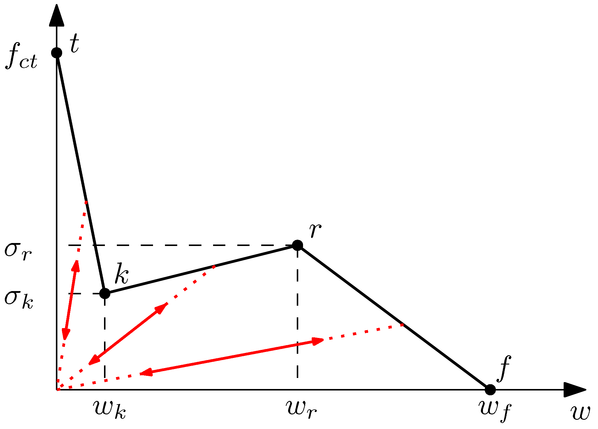
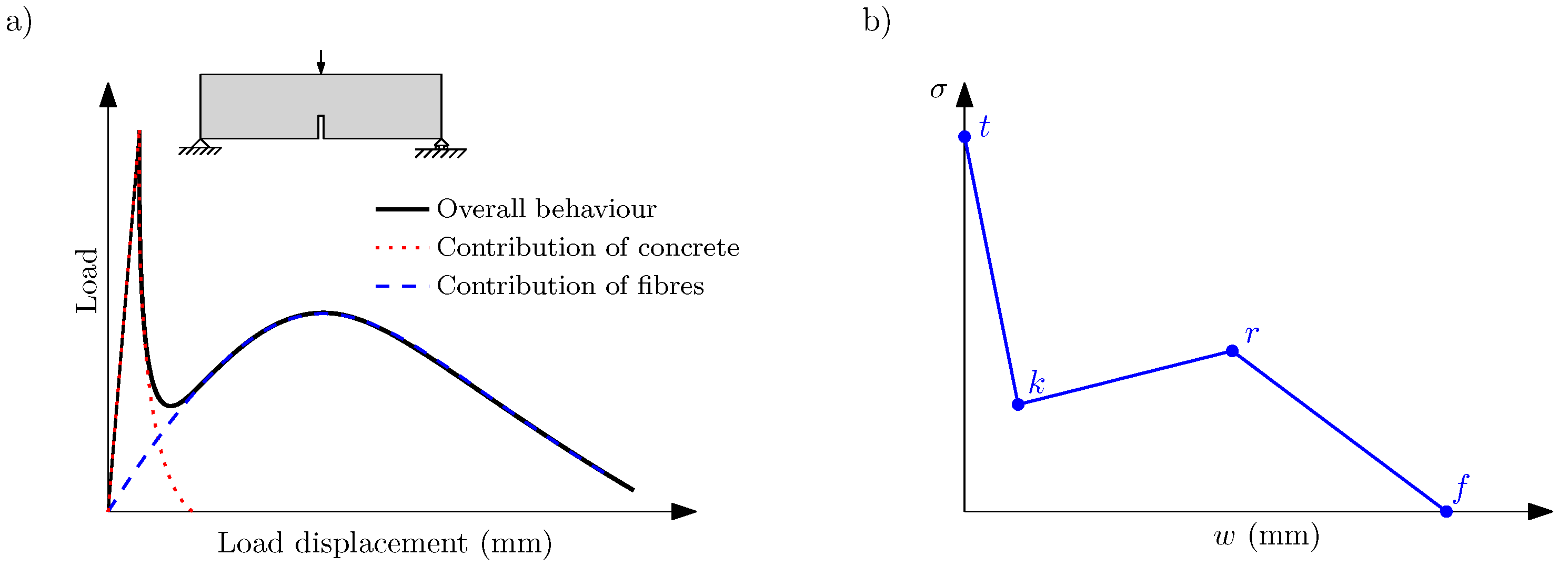
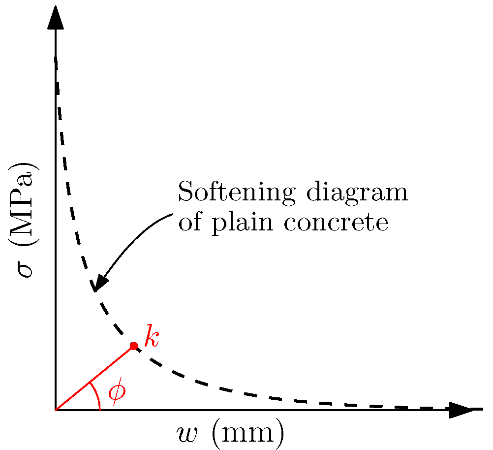
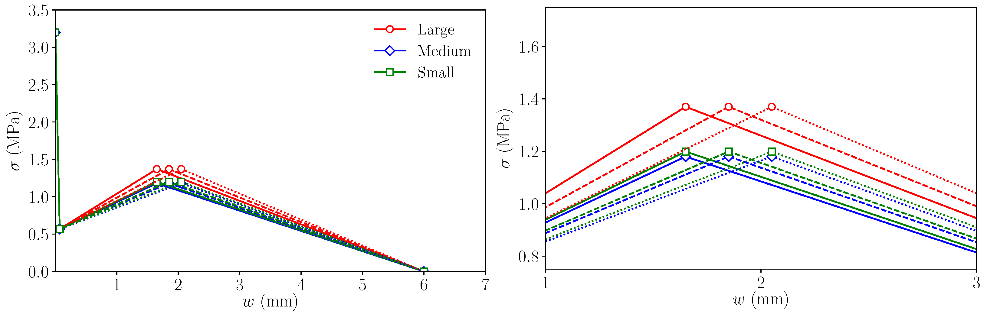
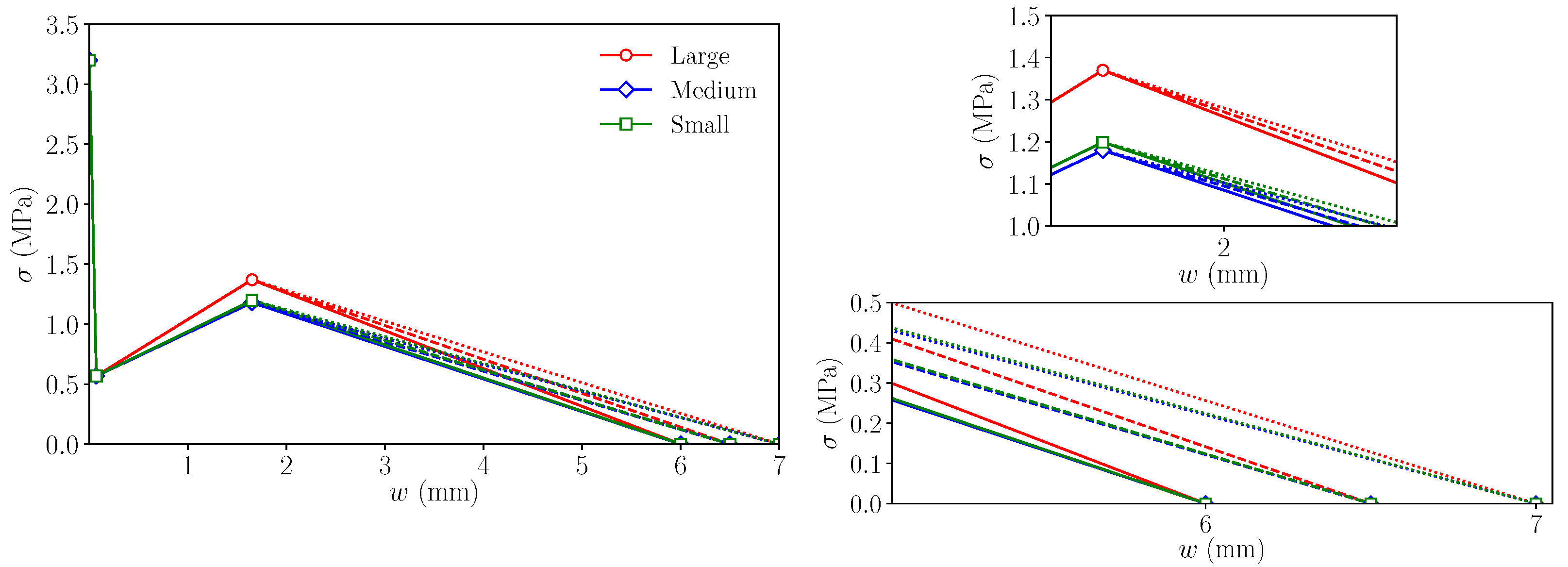
- The complete fracture behaviour of PFRC specimens can be numerically simulated using a predictive trilinear cohesive crack model, which can be defined a priori by means of empirical expressions obtained with lab tests different from those simulated. This diagram is defined by four points, with coordinates that depend on PFRC mechanical characteristics, i.e., the tensile strength of the matrix, the proportion of fibres, and the orientation factor. Abscissa values and (see Figure 3) are fixed based on experimental results obtained in previous literature. It is still an unsolved challenge to obtain expressions to estimate and using the mechanical characteristics of the PFRC.
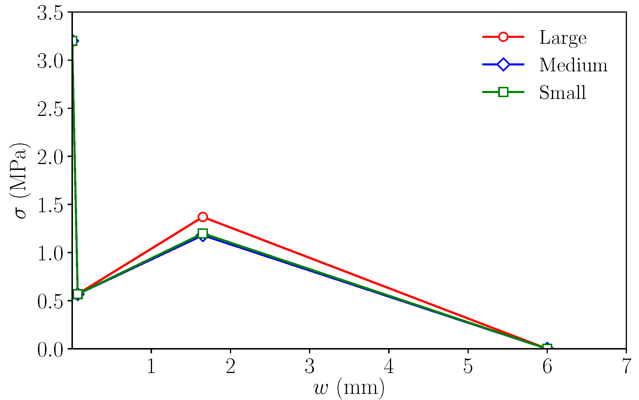
- The softening diagrams are not equal for all specimen sizes and should be adjusted for each of them. This is mainly due to a different orientation factor that varies with the size of the specimen.
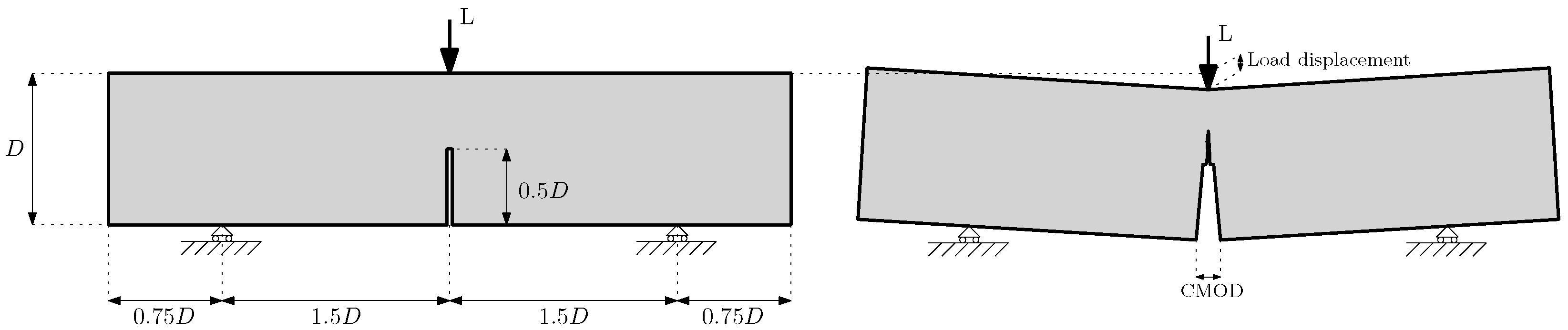
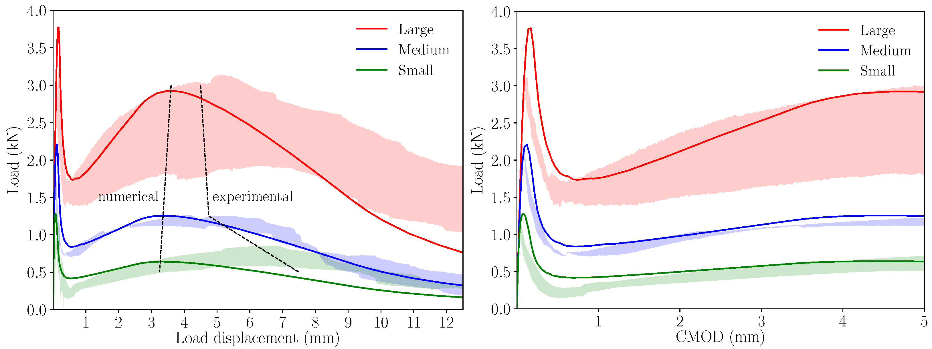
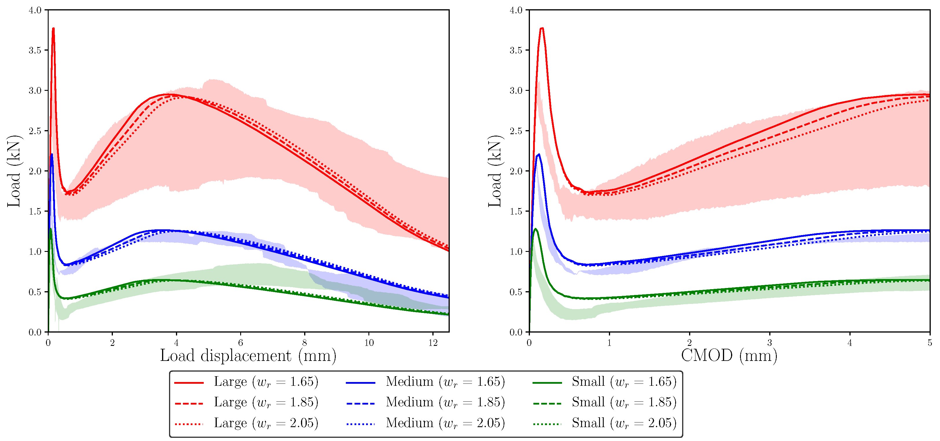
- The maximum remanent loads obtained for each size present a linear trend on the load–displacement diagram, which does not agree completely with the experimental observations, although the load–displacement and load–CMOD curves properly agree with the experimental envelopes for the three studied sizes.
- Modifying and affects the maximum remanent load on the load–displacement diagram and modifies the last part of this diagram but cannot capture the nonlinear trend of the remanent load among specimen sizes.
Author Contributions
Funding
Institutional Review Board Statement
Informed Consent Statement
Data Availability Statement
Conflicts of Interest
References
- Bažant, Z.P. Size effect in blunt fracture: Concrete, rock, metal. J. Eng. Mech. 1984, 110, 518–535. [Google Scholar] [CrossRef]
- Bažant, Z.P.; Planas, J. Fracture and Size Effect in Concrete and Other Quasibrittle Materials; CRC Press: Boca Raton, FL, USA, 1997. [Google Scholar]
- Planas, J.; Guinea, G.; Elices, M. Size effect and inverse analysis in concrete fracture. Int. J. Fract. 1999, 95, 367. [Google Scholar] [CrossRef]
- Jirásek, M.; Rolshoven, S.; Grassl, P. Size effect on fracture energy induced by non-locality. Int. J. Numer. Anal. Methods Geomech. 2004, 28, 653–670. [Google Scholar] [CrossRef]
- Bažant, Z.P.; Yu, Q. Universal size effect law and effect of crack depth on quasi-brittle structure strength. J. Eng. Mech. 2009, 135, 78–84. [Google Scholar] [CrossRef] [Green Version]
- Ward, R.; Li, V. Dependence of flexural behaviour of fibre reinforced mortar on material fracture resistance and beam size. Constr. Build. Mater. 1991, 5, 151–161. [Google Scholar] [CrossRef] [Green Version]
- Di Prisco, M.; Lamperti, M.; Lapolla, S.; Khurana, R.S. HPFRCC thin plates for precast roofing. In Proceedings of the 2nd International Symposium on HPC, Kassel, Germany, 5–7 March 2008. [Google Scholar]
- Shah, S.P.; Rangan, B.V. Fiber reinforced concrete properties. J. Proc. 1971, 68, 126–137. [Google Scholar]
- Zollo, R.F. Fiber-reinforced concrete: An overview after 30 years of development. Cem. Concr. Compos. 1997, 19, 107–122. [Google Scholar] [CrossRef]
- Banthia, N.; Gupta, R. Influence of polypropylene fiber geometry on plastic shrinkage cracking in concrete. Cem. Concr. Res. 2006, 36, 1263–1267. [Google Scholar] [CrossRef]
- Brandt, A.M. Fibre reinforced cement-based (FRC) composites after over 40 years of development in building and civil engineering. Compos. Struct. 2008, 86, 3–9. [Google Scholar] [CrossRef]
- Alberti, M.; Enfedaque, A.; Gálvez, J. Comparison between polyolefin fibre reinforced vibrated conventional concrete and self-compacting concrete. Constr. Build. Mater. 2015, 85, 182–194. [Google Scholar] [CrossRef]
- Alberti, M.; Enfedaque, A.; Gálvez, J.; Cortez, A. Optimisation of fibre reinforcement with a combination strategy and through the use of self-compacting concrete. Constr. Build. Mater. 2020, 235, 117289. [Google Scholar] [CrossRef]
- Alberti, M.; Enfedaque, A.; Gálvez, J. Fibre reinforced concrete with a combination of polyolefin and steel-hooked fibres. Compos. Struct. 2017, 171, 317–325. [Google Scholar] [CrossRef]
- Alberti, M.; Enfedaque, A.; Gálvez, J.; Agrawal, V. Fibre distribution and orientation of macro-synthetic polyolefin fibre reinforced concrete elements. Constr. Build. Mater. 2016, 122, 505–517. [Google Scholar] [CrossRef]
- Alberti, M.; Enfedaque, A.; Gálvez, J.; Reyes, E. Numerical modelling of the fracture of polyolefin fibre reinforced concrete by using a cohesive fracture approach. Compos. Part B Eng. 2017, 111, 200–210. [Google Scholar] [CrossRef]
- Picazo, A.; Gálvez, J.; Alberti, M.; Enfedaque, A. Assessment of the shear behaviour of polyolefin fibre reinforced concrete and verification by means of digital image correlation. Constr. Build. Mater. 2018, 181, 565–578. [Google Scholar] [CrossRef]
- Alberti, M.G.; Gálvez, J.C.; Enfedaque, A.; Carmona, A.; Valverde, C.; Pardo, G. Use of Steel and Polyolefin Fibres in the La Canda Tunnels: Applying MIVES for Assessing Sustainability Evaluation. Sustainability 2018, 10, 4765. [Google Scholar] [CrossRef] [Green Version]
- Enfedaque, A.; Alberti, M.G.; Gálvez, J.C.; Rivera, M.; Simón-Talero, J. Can Polyolefin Fibre Reinforced Concrete Improve the Sustainability of a Flyover Bridge? Sustainability 2018, 10, 4583. [Google Scholar] [CrossRef] [Green Version]
- di Prisco, M.; Felicetti, R.; Lamperti, M.; Menotti, G. On size effect in tension of SFRC thin plates. Fract. Mech. Concr. Struct. 2004, 2, 1075–1082. [Google Scholar]
- Yoo, D.Y.; Banthia, N.; Yang, J.M.; Yoon, Y.S. Size effect in normal- and high-strength amorphous metallic and steel fiber reinforced concrete beams. Constr. Build. Mater. 2016, 121, 676–685. [Google Scholar] [CrossRef]
- Picazo, Á.; Alberti, M.G.; Gálvez, J.C.; Enfedaque, A.; Vega, A.C. The Size Effect on Flexural Fracture of Polyolefin Fibre-Reinforced Concrete. Appl. Sci. 2019, 9, 1762. [Google Scholar] [CrossRef] [Green Version]
- Enfedaque, A.; Alberti, M.; Gálvez, J.; Domingo, J. Numerical simulation of the fracture behaviour of glass fibre reinforced cement. Constr. Build. Mater. 2017, 136, 108–117. [Google Scholar] [CrossRef]
- Suárez, F.; Gálvez, J.; Enfedaque, A.; Alberti, M. Modelling fracture on polyolefin fibre reinforced concrete specimens subjected to mixed-mode loading. Eng. Fract. Mech. 2019, 211, 244–253. [Google Scholar] [CrossRef]
- Enfedaque, A.; Alberti, M.G.; Gálvez, J.C. Influence of Fiber Distribution and Orientation in the Fracture Behavior of Polyolefin Fiber-Reinforced Concrete. Materials 2019, 12, 220. [Google Scholar] [CrossRef] [Green Version]
- European Committee for Standardization. EN 14651: 2005+ A1:2007—Test Method for Metallic Fibre Concrete. Measuring the Flexural Tensile Strength (Limit of Proportionality (LOP), Residual); European Committee for Standardization: Bruxelles, Belgium, 2007. [Google Scholar]
- Hillerborg, A.; Modéer, M.; Petersson, P.E. Analysis of crack formation and crack growth in concrete by means of fracture mechanics and finite elements. Cem. Concr. Res. 1976, 6, 773–781. [Google Scholar] [CrossRef]
- Dugdale, D.S. Yielding of steel sheets containing slits. J. Mech. Phys. Solids 1960, 8, 100–104. [Google Scholar] [CrossRef]
- Barenblatt, G.I. The mathematical theory of equilibrium cracks in brittle fracture. In Advances in Applied Mechanics; Elsevier: Amsterdam, The Netherlands, 1962; Volume 7, pp. 55–129. [Google Scholar]
- Sancho, J.; Planas, J.; Cendón, D.; Reyes, E.; Gálvez, J. An embedded crack model for finite element analysis of concrete fracture. Eng. Fract. Mech. 2007, 74, 75–86. [Google Scholar] [CrossRef]
- Gálvez, J.; Planas, J.; Sancho, J.; Reyes, E.; Cendón, D.; Casati, M. An embedded cohesive crack model for finite element analysis of quasi-brittle materials. Eng. Fract. Mech. 2013, 109, 369–386. [Google Scholar] [CrossRef] [Green Version]
- Reyes, E.; Gálvez, J.; Casati, M.; Cendón, D.; Sancho, J.; Planas, J. An embedded cohesive crack model for finite element analysis of brickwork masonry fracture. Eng. Fract. Mech. 2009, 76, 1930–1944. [Google Scholar] [CrossRef] [Green Version]
- Smith, M. ABAQUS/Standard User’s Manual, Version 6.9; Dassault Systèmes Simulia Corp: Johnston, RI, USA, 2009. [Google Scholar]
- Elices, M.; Guinea, G.; Gómez, J.; Planas, J. The cohesive zone model: Advantages, limitations and challenges. Eng. Fract. Mech. 2002, 69, 137–163. [Google Scholar] [CrossRef]


| Material | SCC10 |
|---|---|
| Cement (kg/m) | 375 |
| Limestone (kg/m) | 200 |
| Water (kg/m) | 188 |
| w/c | 0.5 |
| Gravel (kg/m) | 245 |
| Grit (kg/m) | 367 |
| Sand (kg/m) | 918 |
| Superplasticizer (% cement) | 1.25 |
| PF48 (kg/m) | 10 |

| Material density (g/cm) | 0.910 |
| Eq. diameter (mm) | 0.903 |
| Tensile strength (MPa) | >500 |
| Modulus of elasticity (GPa) | >9 |
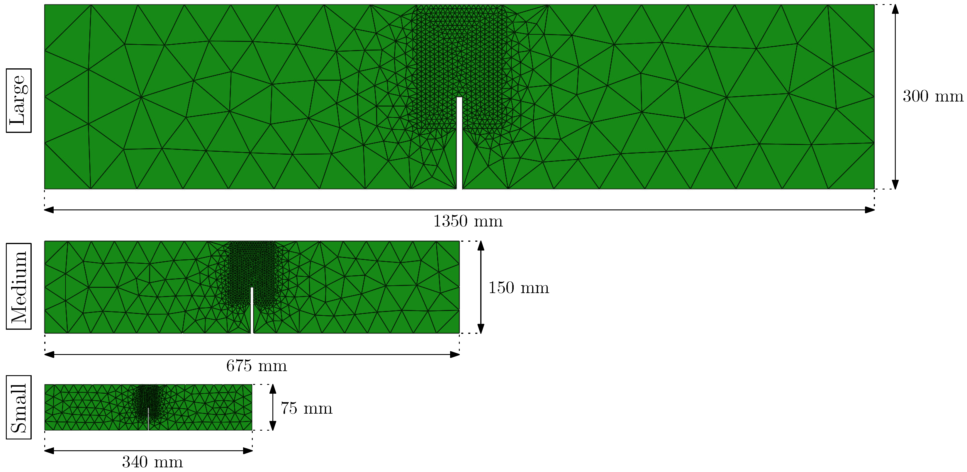
| Specimen | Length (mm) | Width (mm) | Height (mm) | Notch (mm) |
|---|---|---|---|---|
| Large | 1350 | 50 | 300 | 150 |
| Medium | 675 | 50 | 150 | 75 |
| Small | 340 | 50 | 75 | 37.5 |
| (MPa) | (N/mm) | (mm) | (MPa) | ||
|---|---|---|---|---|---|
| Small/Medium/Large | 3.2 | 0.13 | 1.448 | 0.07143 | 0.57715 |
| (MPa) | (MPa) | ||||
|---|---|---|---|---|---|
| Small | 0.63 | 0.54 | 0.011 | 376 | 1.20 |
| Medium | 0.62 | 0.54 | 0.011 | 376 | 1.18 |
| Large | 0.72 | 0.54 | 0.011 | 376 | 1.37 |
| Small | Medium | Large | |
|---|---|---|---|
| (mm) | 0.00 | 0.00 | 0.00 |
| (MPa) | 3.20 | 3.20 | 3.20 |
| (mm) | 0.07 | 0.07 | 0.07 |
| (MPa) | 0.57 | 0.57 | 0.57 |
| (mm) | 1.650 | 1.650 | 1.650 |
| (MPa) | 1.20 | 1.18 | 1.37 |
| (mm) | 6.00 | 6.00 | 6.00 |
| (MPa) | 0.00 | 0.00 | 0.00 |
Publisher’s Note: MDPI stays neutral with regard to jurisdictional claims in published maps and institutional affiliations. |
© 2021 by the authors. Licensee MDPI, Basel, Switzerland. This article is an open access article distributed under the terms and conditions of the Creative Commons Attribution (CC BY) license (https://creativecommons.org/licenses/by/4.0/).
Share and Cite
Suárez, F.; Gálvez, J.C.; Alberti, M.G.; Enfedaque, A. Fracture and Size Effect of PFRC Specimens Simulated by Using a Trilinear Softening Diagram: A Predictive Approach. Materials 2021, 14, 3795. https://doi.org/10.3390/ma14143795
Suárez F, Gálvez JC, Alberti MG, Enfedaque A. Fracture and Size Effect of PFRC Specimens Simulated by Using a Trilinear Softening Diagram: A Predictive Approach. Materials. 2021; 14(14):3795. https://doi.org/10.3390/ma14143795
Chicago/Turabian StyleSuárez, Fernando, Jaime C. Gálvez, Marcos G. Alberti, and Alejandro Enfedaque. 2021. "Fracture and Size Effect of PFRC Specimens Simulated by Using a Trilinear Softening Diagram: A Predictive Approach" Materials 14, no. 14: 3795. https://doi.org/10.3390/ma14143795
APA StyleSuárez, F., Gálvez, J. C., Alberti, M. G., & Enfedaque, A. (2021). Fracture and Size Effect of PFRC Specimens Simulated by Using a Trilinear Softening Diagram: A Predictive Approach. Materials, 14(14), 3795. https://doi.org/10.3390/ma14143795