3D CFD Analysis of a Vertical Axis Wind Turbine

Abstract

To analyze the complex and unsteady aerodynamic flow associated with wind turbine functioning, computational fluid dynamics (CFD) is an attractive and powerful method. In this work, the influence of different numerical aspects on the accuracy of simulating a rotating wind turbine is studied. In particular, the effects of mesh size and structure, time step and rotational velocity have been taken into account for simulation of different wind turbine geometries. The applicative goal of this study is the comparison of the performance between a straight blade vertical axis wind turbine and a helical blade one. Analyses are carried out through the use of computational fluid dynamic ANSYS^® Fluent^® software, solving the Reynolds averaged Navier–Stokes (RANS) equations. At first, two-dimensional simulations are used in a preliminary setup of the numerical procedure and to compute approximated performance parameters, namely the torque, power, lift and drag coefficients. Then, three-dimensional simulations are carried out with the aim of an accurate determination of the differences in the complex aerodynamic flow associated with the straight and the helical blade turbines. Static and dynamic results are then reported for different values of rotational speed.

1. Introduction

In recent decades, the prospect of the depletion of fossil fuels has directed attention toward renewable energy sources. Among the renewable energy sources, onshore wind power is one of the most attractive because of its low cost of maintenance of installed systems. Although the concept of vertical axis wind turbines (VAWTs) was proposed by Darrieus [1] as early as 1931, the research and development in this area are still of interest and in progress nowadays. Among the several categories of wind generators, small wind turbines have gained more and more interest for their excellent adaptability to the urban environment in terms of visual impact and noise pollution. Being axisymmetric, they are omnidirectional turbines, which respond well to changes in wind direction. In order to determine the performance of the VAWT, analytical and numerical approaches, as well as experimental tests are generally used [2–11]. Among others, Sutherland et al. [2] report on the streamtube model and vortex models that allow one to analyze the aerodynamic response of VAWTs. Islam et al. [3] analyzed three aerodynamic models used for the performance prediction and design of a straight blade Darrieus turbine. These three models are the double-multiple streamtube model, free vortex model and cascade model, and we highlight their strengths and weaknesses. The first simplest approach developed by Templin [4] is the single streamtube numerical model. Templin calculates the performance for a single blade whose chord equals the sum of the chords of the actual rotor’s blade; airfoil characteristics are introduced through the application of blade element theory. This approach gives predictions of rotor performance in terms of average torque per revolution only. Strickland [12] extends Templin’s approach into a multiple single streamtube model by considering a number of adjacent smaller streamtube, applying the conservation of momentum and blade element theory to each streamtube. This allows one to determine the performance considering the local Reynolds number rather than an average. Further improvement in the multiple streamtube model has been reported by Paraschivoiu [5], namely the double multiple streamtube model (DSMT); the difference with respect to Strickland’s model is that upwind and downwind passages through each streamtube are considered separately. Low solidity with a low chord-radius ratio (c/r ≤ 0.1) can be modeled well using a DMST analysis, such as the one developed by Paraschivoiu [5]. Brusca et al. [6], using a calculation code based on the multiple stream tube model, analyze the link between the aspect ratio of a VAWT with straight blade; it was highlighted that the power coefficient is influenced by both rotor solidity and the Reynolds number, concluding that a low aspect ratio has several advantages compared to higher ratio values. A second class of models is those based on vortex representation of the blades and their wakes. Strickland et al.’s model [7] is based on replacement of the rotor blade by a bound vortex filament, called a lifting line, whose strength is a function of the azimuthal position. Wang et al.[8] present a potential flow 2D vortex panel model (VPM2D) applied to the vertical axis straight blade variable pitch turbine; however, this model does not include the consideration of the phenomenon of dynamic stall. Experimental tests can be performed by means of wind tunnel or open-field measurement in order to evaluate the real performance of wind turbines. Sheldahl [9] tested a 2-m diameter Darrieus VAWT with NACA-0012 airfoil blades, in the field at the Sandia National Laboratories, and operated it to determine if the data obtained from these tests are comparable with wind tunnel data obtained under ideal conditions. Bedon et al. [10] describe the results of an experimental campaign of measurements conducted on a VAWT with helical blade having a radius of 1 m with a NACA-0018 airfoil section, tested in an open field. With the advent of computers, many authors have investigated the feasibility and accuracy of different computational fluid dynamics (CFD) approaches. Analytical and numerical investigations were conducted by Biadgo et al. [11] on straight blade VAWT using NACA0012 as a blade profile. The analytical investigation is performed using the double-multiple streamtube model, while the numerical investigation of two-dimensional unsteady flow is carried out using CFD. Wolfe et al. [13] use CFD to investigate the two-dimensional aerodynamic performance of typical wind turbine airfoils with the standard κ − ϵ [14] turbulence model, concluding that this model is not appropriate at angles of attack with flow separation. Carrigan et al. [15], fixing the tip speed ratio (TSR) of the wind turbine, developed an iterative design system to maximize the torque for different airfoil cross-sections and solidities in two-dimensional CFD simulations. The TSR, which is also referred to as λ in the manuscript, is defined as U/V_∞, where U is the tip peripheral velocity of the rotor, namely ωR, ω is the angular velocity of the blade and R the rotor radius, while V_∞ is the free stream velocity. A 2.5D model [16] is also presented in the literature, which differs from a 3D simulation, because only a segment of the airfoil blades is modeled with periodic boundaries at the extremities of the domain. The limitation of this model is that it can only be used with Darrieus-type straight-bladed VAWT. Furthermore, although this modeling approach produces a more realistic three-dimensional vortex diffusion after flow separation, it cannot capture the effect of tip vortex and vertical flow divergence in VAWT. These two processes are the major cause of over-prediction of VAWT power in the two-dimensional model [17]. A CFD performance model based on blade element momentum theory was presented by Raciti Castelli et al. [18] for evaluating the aerodynamic forces of straight blade VAWT. Most of the authors have the adopted Reynolds averaged Navier–Stokes equations (RANS) approach with different turbulence models [19,20]. However, Iida et al. [21] used a model with large eddy simulations (LES), proving that the as-obtained results are in good agreement at high TSR with that of momentum theory, but the model was revealed to be not accurate for low TSR cases. Ferreira et al. [22] use detached eddy simulation (DES) focusing on 2D dynamic stall and validate the results with particle image velocimetry data. It is to be noted that in the Darrieus-type VAWT, a cyclic phenomenon of dynamic stall and vortex separation is present [8,22,23]. Amet et al. [23] provided a detailed numerical analysis of the physical phenomena that occur during dynamic stall where the compressible RANS κ − ω model and multi-block mesh structure were used. Furthermore, studies of dynamic stall show that the Shear Stress Transport (SST) κ − ω turbulence model performs better than the κ − ω model, as reported by Ekaterinaris and Platzer [24] and Qian et al. [25]. Only recently have some researchers carried out three-dimensional CFD simulations [26,27]. Howell et al. [26] provided a three-dimensional CFD model based on the Re-Normalisation Group (RNG) κ − ϵ turbulence model, and the effects of turbine solidity, roughness and tip vortices were considered. Zhang et al. [27], analyze a three-bladed straight wind turbine, using a NACA 0015 airfoil with a chord length of 0.4 m and a blade length of 2 m with 4 m in diameter. The aim of the present paper is to numerically compare different Darrieus turbine configurations that differ for the twist angle of the blades. In Section 2, a two-dimensional dynamic numerical model is explained, and the results are: (i) the influence of the rotational domain mesh; (ii) the airfoil behavior; and (iii) the ideal dynamic torque coefficient. In Section 3, a three-dimensional Darrieus turbine configuration and computational domain are described. Then, static analyses are carried out to compute the static performance of the studied configurations, namely the torque produced by the still turbine. Dynamic simulations are also performed to compare the straight blade turbines with the select twisted blade ones in terms of torque and power coefficients during operative cycles. It is to note that, in order to perform the simulations, the κ − ϵ model is employed; this model does not befit analyzing strong adverse pressure gradients. Nevertheless, its strength is given by the reduced calculation times required to perform a simulation with good levels of convergence [28]. Last, conclusions are given in Section 4.

2. Two-Dimensional Model and Results

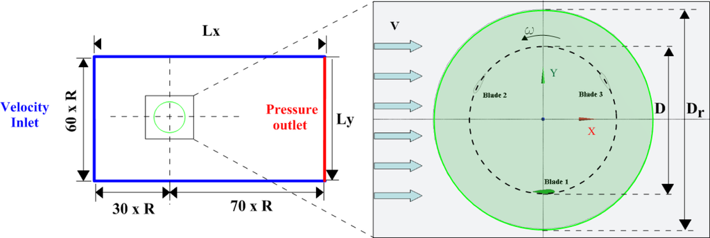
In this section, the geometrical features of the analyzed Darrieus turbine are described first. Then, the adopted control volumes and the corresponding boundary conditions are described. The mesh generation parameters are also given. The solid geometry was created with a CAD modeler and imported into a “Mesh Component Systems” in ANSYS^® Workbench™, to create the mesh model. The discretized model generated was then read into FLUENT^® for numerical solution. The geometric characteristics for the turbine are a NACA 0021 blade airfoil, with a chord length c = 0.3 m and a rotor radius R = 0.99 m. The length of the control volume along the free-stream direction is equal to Lx = 100 R, while its width in the y direction is Ly = 60 R. The circular rotating domain has an overall diameter of D_r = 3 m; see Figure 1. At the velocity inlet, the velocity distribution is uniform, directed along the x-axis and equal to 7 m/s. The pressure outlet is set equal to 101,325 Pa. The no slip boundary condition is applied on the turbine wall blades. An interface wall is introduce between the fixed and rotating domain. The origin of the reference frame is the center of the rotor.

In the present section, the results obtained from the two-dimensional analyses are shown. Transient analyses are carried out in this section to characterize the performances of the investigated airfoil. Performances are described in terms of torque and power coefficients, which are computed using procedures described in [29]. The total torque vector about the rotor axis is computed by summing the elemental cross products of the pressure and viscous force vectors times the vector $\overrightarrow{r}$, that is the distance between the element centroid and the rotor axis; see [30], page 692. Equation (1) represents the pressure and viscous torque vectors:

$$\overrightarrow{T}(\theta )=\overrightarrow{r}\times {\overrightarrow{F}}_p(\theta )+\overrightarrow{r}\times {\overrightarrow{F}}_v(\theta )$$

(1)

where ${\overrightarrow{F}}_p$ is the pressure force vector and ${\overrightarrow{F}}_v$ is the viscous force vector. The instantaneous torque coefficient C_t is defined as:

$$C_t(\theta )=\frac{T(\theta )}{0.5\rho V_{\infty }^2{A}_{S}R}$$

(2)

where ρ is the density, A_S is the size of turbine equal to the product of diameter D and rotor height H and V_∞ is the free stream velocity. For two-dimensional simulation, H is unitary. The average torque coefficient C_t,ave is computed by averaging C_t (θ) over a whole revolution. A minimum of fifteen revolutions of the rotor have been simulated for each λ. The average power coefficient is computed as C_p,ave = C_t,ave λ, with λ ranging from 0.44 to 2.22, taking into account that for this study, the considered design tip speed ratio is about 1.4.

2.1. Mesh Configurations

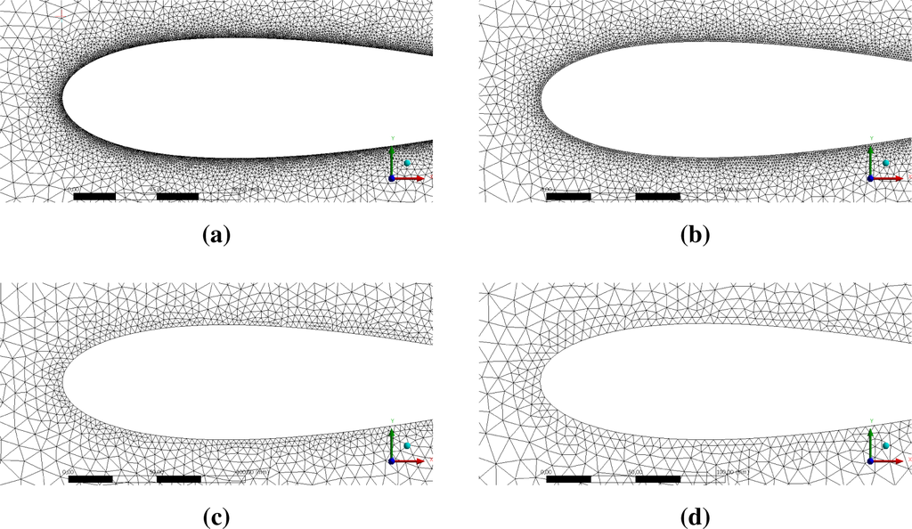
The mesh is characterized by triangular elements; in particular, the maximum element size for the fixed domain is set to 0.5 m, whereas the length of the element at the interface between the fixed and the rotating domain is equal to 0.05 m. The maximum length of the element size close to the airfoils varies between 0.0005 m and 0.005 m for convergence analysis purposes.

The solution model is set using the least-squares cell-based gradient option with second order interpolation method for face pressure. The sliding mesh model [29] is used to model the turbine blade rotation. A multiple reference frame solution [30] is used to compute a flow field as an initial condition for the transient sliding mesh calculation. This eliminates the need for a start-up calculation. The κ − ϵ approach with enhanced wall treatment [31] is adopted to model the flow turbulence.

When using a sliding mesh, it is known [32] that to have a good numeric convergence characteristic, the value of the time step should not be larger than the time it takes for a moving cell to advance of a characteristic length L_c. An estimate for the time step in the case of translational motion can be calculated as Equation (3):

$$\mathrm{\Delta }t=\frac{1}{3}\frac{L_c}{V}$$

(3)

where the step size Δt is proportional to the cell characteristic size L_c and inversely to velocity V. On the other hand, for turbomachinery, the following relation is suggested, Equation (4) [32]:

$$\mathrm{\Delta }t=\frac{1}{10}\frac{Numberofblades}{rotationalvelocity}$$

(4)

Taking into account that the radius of the turbine is equal to that of the rotational sliding computational domain and assuming an angular velocity of 120 RPM, from Equation (3), a value of Δt about equal to 0.001 s is obtained. In applying Equation (3), the characteristic length is L_c = 0.05 m and V = ω R = 18, 85 m/s; whereas from Equation (4), Δt = 0.016 s is obtained. For all two-dimensional simulations, the step size is set equal to 0.0005 s to increase the accuracy of the solution.

At first, the behavior of the two-dimensional turbine as a function of the mesh discretization along the profile is analyzed. In

Table 1. Mesh discretization values.

Name	Length (m)	Airfoil Elements	Domain Node	Domain Elements
Mesh 0	0.0005	1,304	32,901	61,405
Mesh 1	0.001	650	19,081	35,699
Mesh 2	0.003	216	9,732	18,277
Mesh 3	0.005	130	7,614	14,301

are listed the four selected maximum elements lengths, the number of nodes and the number of elements of the control volume and on the airfoil edge, whereas in Figure 2, the mesh grids close to the airfoils are shown.

The influence of discretization is assessed by investigating the effect of the characteristics of the maximum element length close to the airfoil on the torque coefficients C_t. More particularly, it appears from Figure 3 that the torque coefficient for the three blades is only slightly affected by the chosen mesh size values, as well as by the y+ (see [30], page 109), which is lower then 10 for Mesh 0, Mesh 1 and Mesh 2.

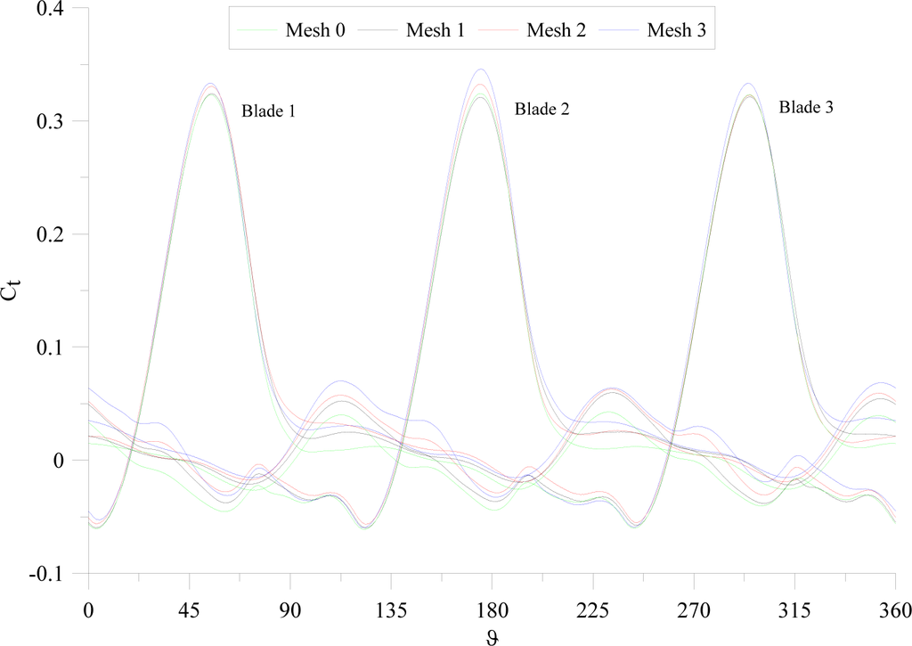
The trend of curve for the individual blade, in a time interval corresponding to one revolution, is shown in Figure 3, for a rotational speed of 60 RPM. With reference to Figure 3, the Mesh 3 and Mesh 2 curves show an overprediction with respect to the Mesh 1 and Mesh 0 data. However, the average discrepancy between Mesh 3 and Mesh 1 is equal to 8.09%, over one revolution, while the value of Mesh 2 with respect to Mesh 1 is equal to 3.91%. Mesh 1 has an average discrepancy of 1.27% with respect to Mesh 0. For this reason, to reduce the computational times, Mesh 2 is selected to carry out the simulations.

2.2. Dynamic Stall Angle

Once the discretization of the mesh along the airfoil is set, two-dimensional simulations with increasing rotational speeds of the blades are carried out. Six different rotational speeds corresponding to λ from 0.44 to 2.22 are chosen; the selected range of velocity allows one to analyze the characteristic bell shape curve that describes the behavior of a Darrieus turbine in terms of the power coefficient [33]. The aim is to investigate the aerodynamic performance behavior.

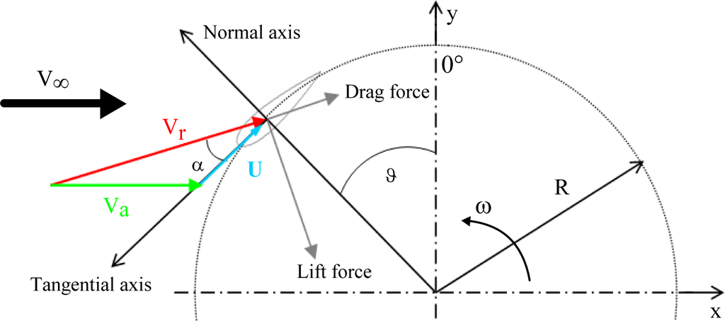
In order to compute the lift and drag coefficients of the blade airfoil, the angle of attack has to be considered, and it is directly computed by the CFD analysis. Taking into account Figure 4, it appears that the angle of attack α is the angle between the airfoil cord and the relative velocity V_r. The relative velocity V_r of the air mass deflected by the airfoils is given by the vectorial composition of the wind velocity V_a with the tangential relative velocity U = −ω R.

By using numerical results for C_x and C_y, the lift and drag coefficients are computed according to:

$$C_l=C_y[\cos (\mathit{\vartheta }+\alpha )]-C_x[\sin (\mathit{\vartheta }+\alpha )]$$

(5)

$$C_d=C_y[\sin (\mathit{\vartheta }+\alpha )]+C_x[\cos (\mathit{\vartheta }+\alpha )]$$

(6)

The lift and drag coefficients’ variation with respect to azimuthal position are reported for different values of the tip speed ratio in Figure 5. It is seen that as the λ increases, both the maximum absolute value of the lift and drag coefficients produced by airfoil increase.

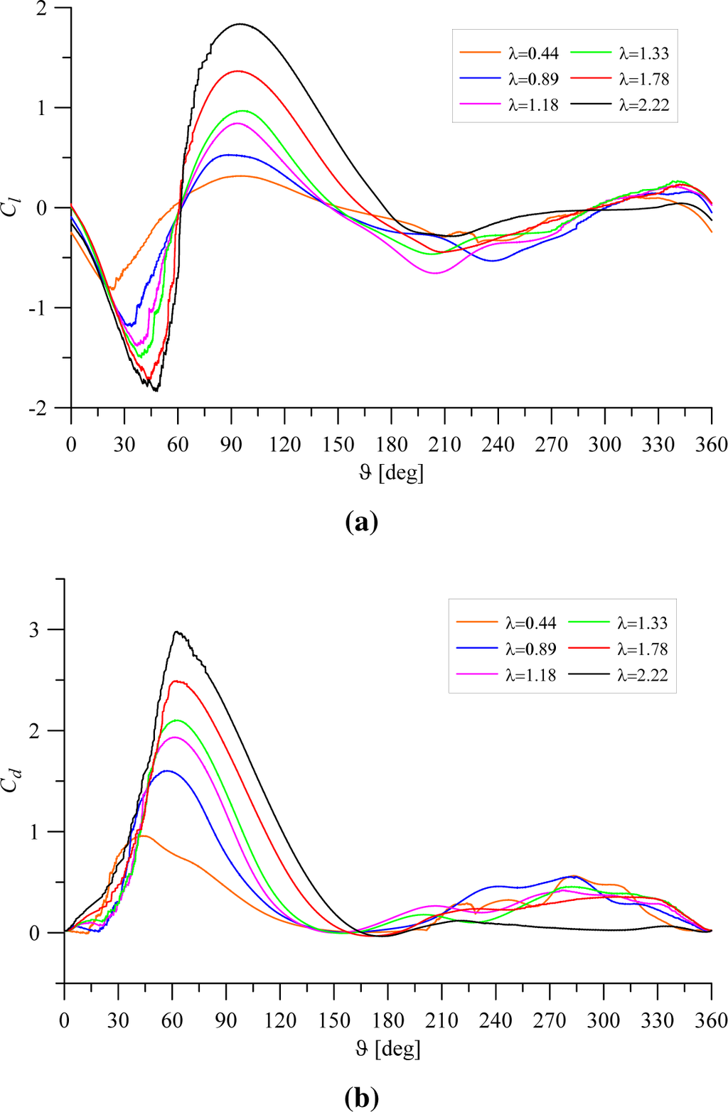
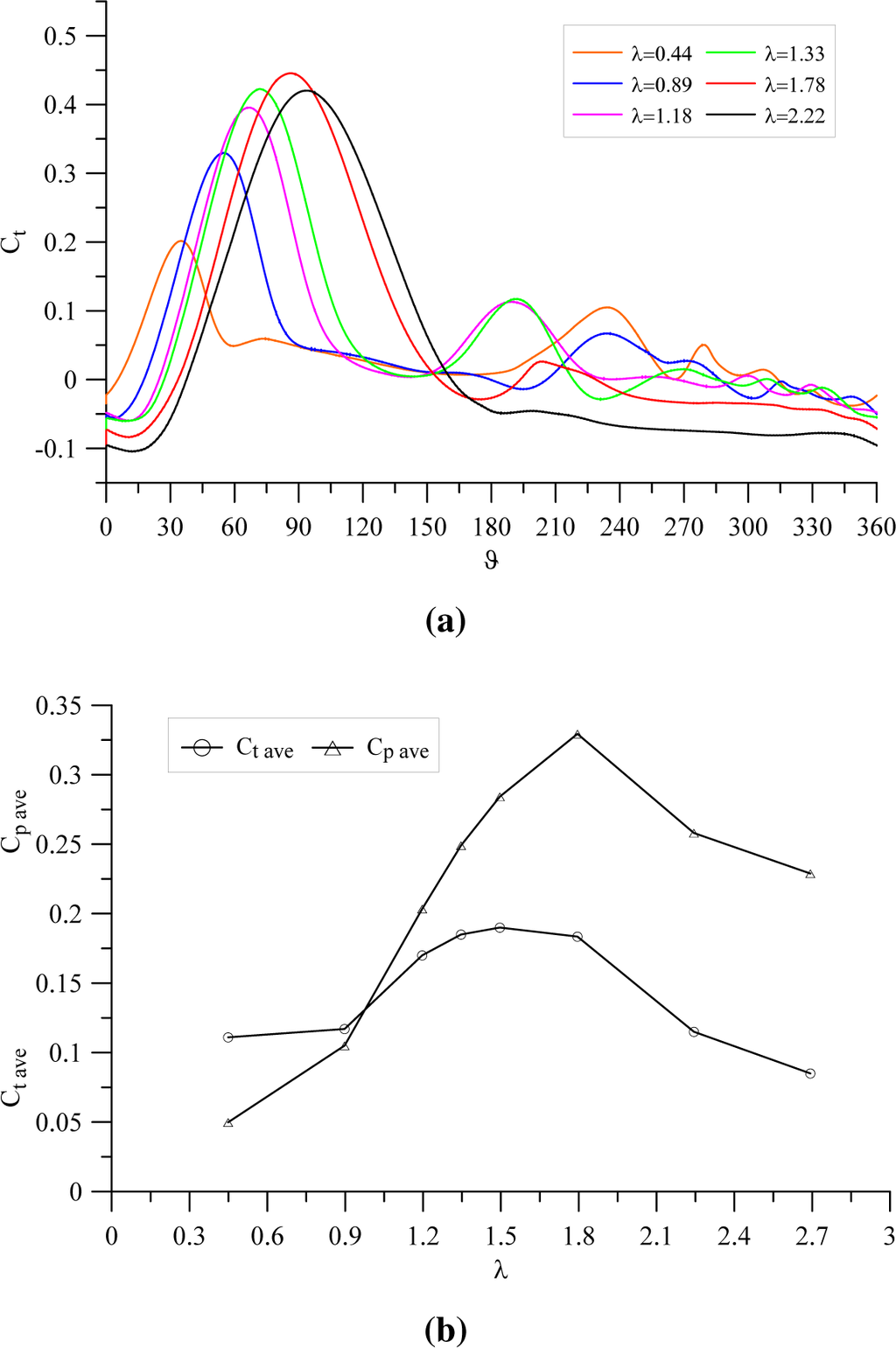
However, by looking at Figure 6a, it appears that the maximum value of torque coefficients is obtained for λ equal to 1.78. This trend is also confirmed by the average distribution of both torque and power coefficients, as appears from Figure 6b.

Summary results are given in

Table 2. Stall and maximum torque data at different λ values.

RPM	λ	αStall	Cl,Stall	θStall	${\alpha }_{C_{t,max}}$	Ct,max	${\theta }_{C_{t,max}}$
30	0.44	1.124	−0.819	23.940	28.905	0.201	35.028
60	0.89	4.088	−1.188	33.948	35.759	0.329	55.044
80	1.18	9.016	−1.381	37.056	40.304	0.395	66.960
90	1.33	11.529	−1.499	39.528	42.622	0.422	71.874
120	1.78	11.760	−1.719	42.912	46.419	0.445	86.904
150	2.22	12.081	−1.834	48.420	44.422	0.420	93.600

in terms of airfoil stall condition and maximum torque coefficients. As λ increases, the azimuthal position where the airfoil stall increases, while the stall angle of attack decreases. Similar results are obtained for the maximum torque coefficient, both in terms of azimuthal position and angle of attack. According to Sheldahl et al. [9], it is found that for a Reynolds number of 355,000, which corresponds to the case λ = 2.22, the stall angle of attack is about 12 degrees, which compares well with our results.

3. Three-Dimensional Models and Results

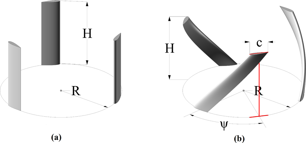
Three-dimensional models are now considered to take into account the finite aspect ratio effects. Four distinct wind turbine configuration are taken into account, namely the Straight blades VAWT and three Helical blades VAWT with different twist angles. The considered twist angles for the Helical blade VAWT are ψ = 30°, 60°, 90°; see Figure 7. The airfoils’ characteristics and rotor diameters are the same for the two-dimensional analyses (NACA 0021, R = 0.99 m), and the rotor height is H = 1.15 m.

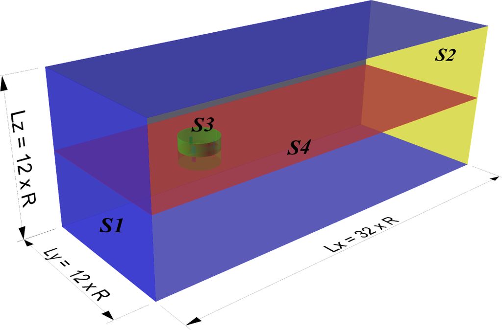
The length of the control volume along the free-stream direction is equal to Lx = 32 R, while its width in the y and z direction is Ly = Lz = 12 R; see Figure 8. The origin of the reference frame is set on the center of the rotor, 8 m from the inlet. The boundary conditions are defined as a velocity inlet on surface S1 in Figure 8; the inflow velocity is directed along the x axis only and equals 7 m/s. Surface S2 is set as a pressure outlet, keeping the pressure constant equal to 101,325 Pa. In Figure 8, surface S3 is the interface between the rotating and the fixed volumes. The no slip boundary condition is applied on the turbine wall blades. The rotational speed of the turbines, for the sake of dynamic analyses, ranges from 30 RPM to 120 RPM. The origin of the reference frame is the center of the rotor; on surface S4 in Figure 8.

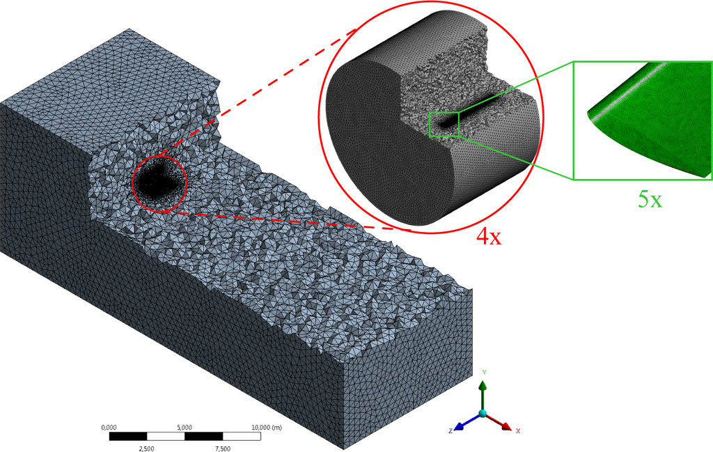
The mesh is characterized by tetrahedral elements. In particular, the maximum element size for the fixed domain is set to 0.5 m; the length of the element at the interface is equal to 0.05 m, whereas the minimum element size is 0.003 m and is used to discretize the fluid domain on the turbine wall; see Figure 9. The number of elements and nodes for the three-dimensional mesh are given in

Table 3. Number of three-dimensional grid nodes and elements.

	Straight (ψ = 0°)	Helical (ψ = 30°)	Helical (ψ = 60°)	Helical (ψ = 90°)
Mesh Node	1,736,475	1,809,898	1,885,205	1,990,686
Mesh Element	9,503,471	9,933,335	10,367,297	10,967,904

.

In the following, results obtained from the three-dimensional analyses are shown. Static and transient analyses are carried out in this section to characterize the performances of the investigated wind rotors. The performance of Darrieus wind turbine is described in terms of moment coefficients, which are computed using procedures described in [29]. On the other hand, dynamical wind turbine performances are obtained by computing the average torque coefficients, over an operational cycle of the rotor.

3.1. Static 3D Comparison

Initially, static simulations are carried out to characterize the behavior of the turbine blade considering rigid rotations with steps of 10°. Because of the rotational symmetry of the geometry, only one blade is considered. Static results for Blade 2 and Blade 3 differ from Blade 1 data for a phase shift of +120° and −120°, respectively. The curves corresponding to the single blade are shown in Figure 10b, respectively for the Straight and Helical configurations. Figure 10a instead shows the three-blade curve trend. It can be seen that the curve of the Helical blade is smoother than that of the Straight blade. This is due to the fact that the Straight blade has an optimal angular position with respect to the relative wind corresponding to 30°, while the Helical blade always presents a section in the optimal position with respect to the relative wind. This becomes more noticeable with increasing twist angle. Moreover, the mean torque for the Helical blade results are greater than the one for the Straight blade for the Helical(ψ = 60°) and Helical(ψ = 90°) configurations. Instead, there is a decrease in mean performance for Helical(ψ = 30°), as shown in

Table 4. Comparison of the average torque coefficient between ψ = 0°, 30°, 60°, 90°.

Configuration	Turbine Ct Average	Variance	Blade Ct Average	Variance	$100{\left(\frac{C_{tH}}{C_{tS}}-1\right)}^1$
Straight (ψ = 0°)	0.107	0.001282	0.0359	0.001347	–
Helical (ψ = 30°)	0.105	0.000500	0.0352	0.001109	−2.09
Helical (ψ = 60°)	0.117	0.000077	0.0391	0.000701	8.75
Helical (ψ = 90°)	0.124	0.000049	0.0415	0.000588	15.53

¹C_tH refers to Helical C_t average; C_tS refers to Straight C_t average.

.

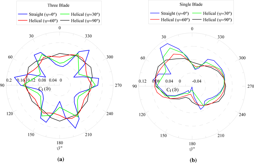
To decide which one of the helical configurations would be the best, not just consideration of the numerical performances should be done. In fact, although a comparison between the ψ = 60° and ψ = 90° Helical VAWT could lead to choosing the ψ = 90° as the best one, the technological point of view must be kept in mind also when manufacturing and installing such turbines. Complications arise in manufacturing highly twisted blades as the ψ = 90°, especially if a fiber composite is used as the bulk material. Furthermore, as the twist angle increases, also the weight increases: this means difficult installing procedures and higher loads on rotating supports. The improvements in performance given in Table 4 from ψ = 60° to ψ = 90° are not so significant to justify the complications previously mentioned. The goal of the paper is to perform a preliminary comparative numerical analysis to be confirmed with a future experimental campaign on turbine prototypes. For these reasons, it has been decided to choose the ψ = 60° turbine as the one to be studied in the following dynamic three-dimensional analysis. Hereinafter, the ψ = 60° VAWT will be the only Helical turbine compared to the Straight one.

3.2. Dynamic Behavior

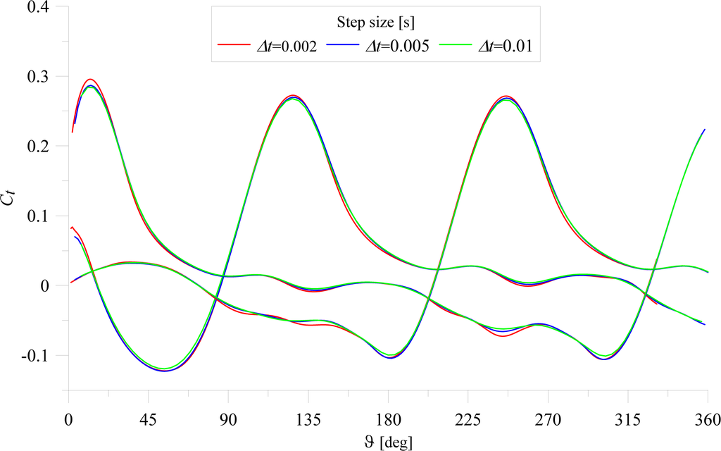
In order to define the time step size for three-dimensional simulations, Equations (3) and (4) are invoked for a rotational speed of 60 RPM resulting in Δt = 0.0017 s and Δt = 0.03 s, respectively. Three different values of step sizes are selected, namely Δt = 0.002, 0.005, 0.01 s. The performance characteristics for the selected time step size are thus investigated. From the results shown in Figure 11, it can be seen that time step equal to 0.01 s allows one to obtain matching results with the finer step sizes. Moreover, the choice of Δt = 0.01 s allows one to reduce the calculation time considerably.

Dynamical wind turbine performances are obtained by computing the instantaneous torque coefficient C_t. Moreover, average torque and power coefficients over an operational cycle of the rotor are shown at the end of this subsection.

Figures 12 and 13 show the trend of the moment coefficient over a full operational cycle. The polar distributions refer to the sum of the three blades and to three different values of RPM, namely 60, 90 and 120.

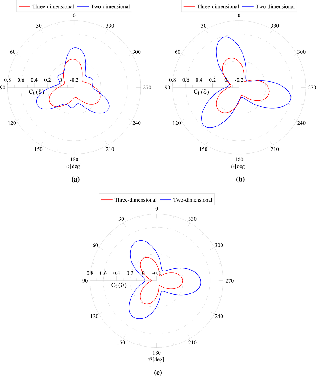
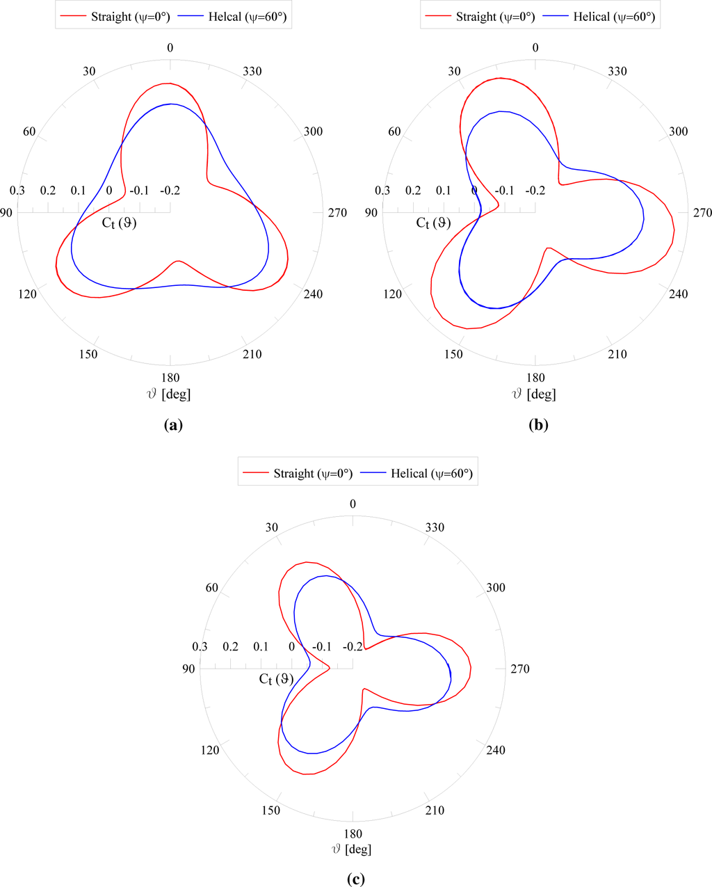
In Figure 12, the comparison between two-dimensional simulations with respect the three-dimensional Straight blade data is presented, whereas a comparison between the three-dimensional Straight blade and Helical(ψ = 60°) blade is given in Figure 13. From the results reported in Figure 12, it appears that a finite turbine three-dimensional blade has a performance reduction linked to vortex diffusion after flow separation; this is in accordance with the literature [17].

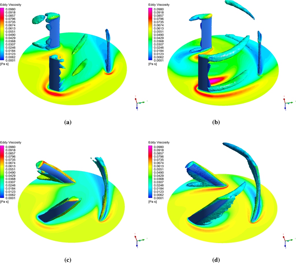
For the sake of completeness and to better highlight this effect, the vortex core regions are shown in Figure 14. It appears that as the rotational speed increases, vortex core regions extend more and more, influencing the upcoming blade. This phenomenon is more evident in the Straight blade geometry (Figure 14), where vortices accumulate mainly at blade tips. On the contrary, in the Helical blade geometry, vortices are evenly distributed along the blade trailing edges. Considering a three-dimensional blade, the Helical blade has a smoother behavior with respect to the Straight blade; as shown in Figure 13, the maximum value of C_t(θ) is obtained at about the same azimuthal position. This effect reduces with the increase of the angular velocity.

For a given free stream velocity, the moment coefficient of Helical blades is greater than the Straight blade configuration, as shown in Figure 15. For higher values of the RPM, the tip vortex diffusion leads to a deterioration of blade performances on the advancing blade with respect to the straight configuration.

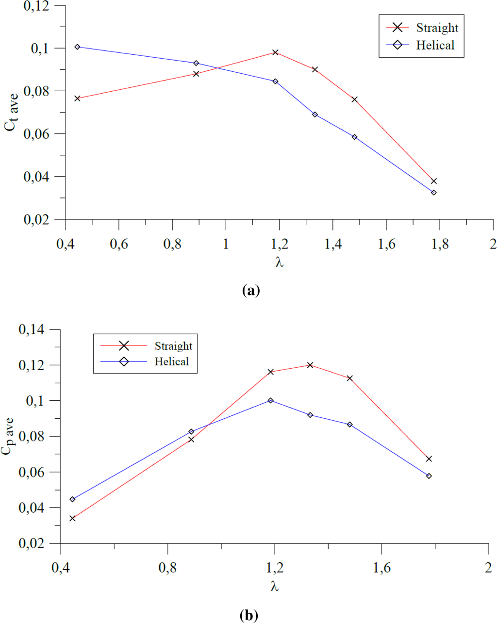
At low rotational speed, the average C_tave for the helical blade turbine is higher with respect to the straight blade up to λ = 1, where the curves intersect. The straight blade configuration produces higher C_tave as the rotational speed increases beyond this value. In accordance with static results for the given conditions, the helical turbine shows a lower cut-in speed.

4. Conclusions

In the present paper, a comparative evaluation of a small Helical-VAWT and of a Straight-VAWT has been performed. Preliminary two-dimensional and subsequent three-dimensional CFD analyses have been carried out. Dynamic two-dimensional simulation data have been collected at different tip speed ratio values, and the results show the torque, lift and drag coefficient behavior of the rotor blade over a revolution with respect to the azimuthal position. Subsequently, three-dimensional static analyses of four different configurations, ψ = 0°, 30°, 60°, 90°, have been performed. Among these, only two configurations, Straight (ψ = 0°) and Helical (ψ = 60°), were used in the dynamic analyses. From steady simulations, over a complete cycle, it has been observed that the Helical blades have an average torque coefficient increment equal to 8.75%. This leads the Helical VAWT to a low speed of start-up (this is confirmed by dynamic results at low rotational speed) and then to a higher number of operational hours in similar environmental conditions. Furthermore, it has been shown, by comparing three-dimensional with two-dimensional results, that the generation of the tip vortices greatly reduces the aerodynamic performance. However, for a three-dimensional comparison, it is shown that this effect is less relevant in the Helical VAWT than in the Straight one.

References

- Darrieus, G. Turbine Having Its Rotating Shaft Transverse to the Flow of the Current. U.S. Patent 1,835,018, 8 December 1931. [Google Scholar]
- Sutherland, H.J.; Berg, D.E.; Ashwill, T.D. A Retrospective of VAWT Technology; Sandia Report, SAND2012-0304; Sandia National Laboratories: Albuquerque, NM, USA; January; 2012. [Google Scholar]
- Islam, M.; Ting, D.S.K.; Fartaj, A. Aerodynamic models for Darrieus-type straight-bladed vertical axis wind turbines. Renew. Sustain. Energy Rev. 2008, 12, 1087–1109. [Google Scholar]
- Templin, R.J. Aerodynamic Performance Theory for the NRC Vertical-Axis Wind Turbine; Technical Report N-76-16618; LTR-LA-160; National Aeronautical Establishment: Ottawa, ON, Canada; 1; June; 1974. [Google Scholar]
- Paraschivoiu, I. Double-multiple streamtube model for studying vertical-axis wind turbines. J. Propuls. Power. 1988, 4, 370–377. [Google Scholar]
- Brusca, S.; Lanzafame, R.; Messina, M. Design of a vertical-axis wind turbine: How the aspect ratio affects the turbine’s performance. Int. J. Energy Environ. Eng. 2014, 5, 333–340. [Google Scholar]
- Strickland, J.; Webster, B.; Nguyen, T. A vortex model of the Darrieus turbine: An analytical and experimental study. J. Fluids Eng 1979, 101, 500–505. [Google Scholar]
- Wang, L.; Zhang, L.; Zeng, N. A potential flow 2-D vortex panel model: Applications to vertical axis straight blade tidal turbine. Energy Convers. Manag. 2007, 48, 454–461. [Google Scholar]
- Sheldahl, R.E. Comparison of field and wind-tunnel Darrieus wind-turbine data. J. Energy. 1981, 5, 254–256. [Google Scholar]
- Bedon, G.; Castelli, M.R.; Benini, E. Experimental tests of a vertical-axis wind turbine with twisted Blades, Proceedings of the 15th International Conference on Mechanical, Industrial, and Manufacturing Engineering, Istanbul, Turkey, 5–6 December 2013.
- Biadgo, M.A.; Simonović, A.; Komarov, D.; Stupar, S. Numerical and analytical investigation of vertical axis wind turbine. FME Trans 2013, 41, 49–58. [Google Scholar]
- Strickland, J.H. Darrieus Turbine: A Performance Prediction Model Using Multiple Streamtubes; Technical Report; Sandia Labs.: Albuquerque, NM, USA, 1975. [Google Scholar]
- Wolfe, W.P.; Ochs, S.S. Predicting Aerodynamic Characteristic of Typical Wind Turbine Airfoils Using CFD; Technical Report; Sandia National Labs.: Albuquerque, NM, USA, 1997. [Google Scholar]
- Launder, B.; Spalding, D. Lectures in Mathematical Models of Turbulence; Academic Press: London, UK, 1972. [Google Scholar]
- Carrigan, T.J.; Dennis, B.H.; Han, Z.X.; Wang, B.P. Aerodynamic shape optimization of a vertical-axis wind turbine using differential evolution. ISRN Renew. Energy. 2012. [Google Scholar] [CrossRef]
- Li, C.; Zhu, S.; Xu, Y.L.; Xiao, Y. 2.5 D large eddy simulation of vertical axis wind turbine in consideration of high angle of attack flow. Renew. Energy. 2013, 51, 317–330. [Google Scholar]
- Hofemann, C.; Ferreira, C.S.; Dixon, K.; van Bussel, G.; van Kuik, G.; Scarano, F. 3D Stereo PIV study of tip vortex evolution on a vawt, Proceedings of the European Wind Energy Conference and Exhibition (EWEC), Brussels, Belgium, 31 March–3 April 2008.
- Raciti Castelli, M.; Englaro, A.; Benini, E. The Darrieus wind turbine: Proposal for a new performance prediction model based on CFD. Energy 2011, 36, 4919–4934. [Google Scholar]
- Castelli, M.R.; Benini, E. Effect of blade inclination angle on a Darrieus wind turbine. J. Turbomach. 2012, 134, 031016. [Google Scholar]
- Lanzafame, R.; Mauro, S.; Messina, M. 2D CFD modeling of H-darrieus wind turbines using a transition Turbulence Model. Energy Procedia 2014, 45, 131–140. [Google Scholar]
- Iida, A.; Kato, K.; Mizuno, A. Numerical simulation of unsteady flow and aerodynamic performance of vertical axis wind turbines with LES, Proceedings of the 16th Australasian Fluid Mechanics Conference (AFMC), Gold Coast, Australia, 2–7 December 2007; pp. 1295–1298.
- Ferreira, C.S.; Bijl, H.; Van Bussel, G.; van Kuik, G. Simulating dynamic stall in a 2D VAWT: Modeling strategy, verification and validation with particle image velocimetry data. J. Phys. Conf. Ser. 2007, 75. [Google Scholar] [CrossRef]
- Amet, E.; Maître, T.; Pellone, C.; Achard, J.L. 2D numerical simulations of blade-vortex interaction in a darrieus turbine. J. Fluids Eng 2009, 131. [Google Scholar] [CrossRef]
- Ekaterinaris, J.A.; Platzer, M.F. Computational prediction of airfoil dynamic stall. Progress Aerosp. Sci. 1998, 33, 759–846. [Google Scholar]
- Qian, W.; Fu, S.; Cai, J. Numerical study of airfoil dynamic stall. Acta Aerodyn. Sin. 2001, 19, 427–433. [Google Scholar]
- Howell, R.; Qin, N.; Edwards, J.; Durrani, N. Wind tunnel and numerical study of a small vertical axis wind turbine. Renew. Energy. 2010, 35, 412–422. [Google Scholar]
- Zhang, L.; Liang, Y.; Liu, X.; Jiao, Q.; Guo, J. Aerodynamic performance prediction of straight-bladed vertical axis wind turbine based on CFD. Adv. Mech. Eng. 2013, 2013. [Google Scholar] [CrossRef]
- Alaimo, A.; Esposito, A.; Milazzo, A.; Orlando, C.; Trentacosti, F. Slotted blades savonius wind turbine analysis by CFD. Energies 2013, 6, 6335–6351. [Google Scholar]
- FLUENT Manual—ANSYS Release Version 14.5, User’s Guide; ANSYS Inc.: Canonsburg, PA, USA, 2012.
- FLUENT Manual—ANSYS Release Version 14.5, Theory Guide; ANSYS Inc.: Canonsburg, PA, USA, 2012.
- Chen, H.; Patel, V. Near-wall turbulence models for complex flows including separation. AIAA J. 1988, 26, 641–648. [Google Scholar]
- FLUENT Training Material—ANSYS Release Version 14.5, Lecture Transient Flow Modeling, Introduction to ANSYS Fluent; ANSYS Inc.: Canonsburg, PA, USA, 2012.
- Paraschivoiu, I. Wind Turbine Design: With Emphasis on Darrieus Concept; Polytechnic International Press: Montreal, QC, Canada, 2002. [Google Scholar]
© 2015 by the authors; licensee MDPI, Basel, Switzerland This article is an open access article distributed under the terms and conditions of the Creative Commons Attribution license (http://creativecommons.org/licenses/by/4.0/).